Blake Group Spectroscopy Tools Software

208

Appendix C

Blake Group Spectroscopy ToolsSoftware

C.1 Main Panel

Blake Group Spectroscopy Tools (BGSpecT) is a set of tools for remote control of

experiments and data collection. It consists of a set of modules, controlling instruments

(C.1.1) and tools (C.1.2) to work with those instruments (i.e., record spectra or some other

signal functions and communicate with instrument devices on low level).

Among the useful features of BGSpecT are that it:

• Simultaneously controls multiple devices of the same kind

• Controls devices via GPIB and RS232 interfaces as well as PC plug-in cards (PCI or

ISA)

• Simultaneously controls multiple GPIB boards

• Incorporates smart oscilloscope waveform acquisition

• Enables wavelength source wavelength conversions

• Can Master/Slave lock delay lines from pulse/delay generator

• Has a huge number of supported oscilloscopes

• Easily enables acquisition of spectra

209

• Can be flexibly configured

• Provides a user friendly interface, with partial Windows XP themes support

The BGSpecT panel itself is a switch board. It is used to turn On/Off the instrument

and tool sub-panels which can only be accessed through the switch board. These sub-panels

may be opened by pressing a corresponding button on the BGSpecT panel.

C.1.1 Instruments

Instrument sub-panels communicate with miscellaneous devices and control them. In-

strument panels are:

• Lambda Tune (C.2) – controls multiple multi-axis lasers via a Motion Control sub-

panel and diode lasers via GPIB and RS232

• Wavemeter (C.3) – controls multiple wavemeters via GPIB and RS232

• Motion Control (C.4) – handles precision motion control micropositioners via PC

plug-in cards (ISA)

210

• Oscilloscope (C.5) – controls multiple oscilloscopes via GPIB, RS232 and PC plug-in

cards (PCI or ISA)

• Delay Generator (C.6) – controls multiple pulsed delay generators via GPIB

• Photon Counter (C.7) – controls multiple photon counters via GPIB and RS232

C.1.2 Tools

The tool sub-panels use either Instrument sub-panels to acquire data and perform data

analysis, or are used as a general tool for Instrument panel devices. Tool panels are:

• Spectrum Scan (C.8) – records spectra using lambda tune sources, motion control

micropositioners and delay generators as sources and oscilloscopes, photon counters and

wavemeters as detectors

• Device Talk (C.9) – configures COM port settings for RS232 communication. Can

talk to GPIB and RS232 devices using individual device commands

C.1.3 Menus

The program menus are:

• File

The “Save Window Configuration” menu saves the current On/Off status for sub-panels.

The “Load Window Configuration” menu loads the above configuration. When exiting, the

program saves the configuration and then loads it automatically the next time it is started.

• Configure

211

Here, one can change the maximum number of allowed devices in the Instrument panels.

Its instrument submenus are disabled if either the corresponding panel or the Spectrum Scan

panel is currently open. The valid number of devices is between 1 and 64. Keeping this

number small (no larger than needed) helps to speed up multi-device tasks such as reading

oscilloscope traces.

The “Classic Theme” menu is enabled only in Windows XP. It switches between the

classic look of the program controls (like that in previous Windows versions) and the partial

XP themes look (when the menu is not checked).

• Help

This provides help for BGSpecT program. A web browser must be installed to view

help files.

C.1.4 System Tray Icon

When the BGSpecT panel is minimized, its icon is placed in a system tray.

It can be restored by double-clicking the icon in the system tray. Right-clicking on the

icon will bring up the following menu that can be used to open/close instrument and tool

panels, restore BGSpecT panel to its normal state, or exit the program.

212

C.1.5 Other

The BGSpecT main directory has 2 sub-directories: Help (where all the help files are

stored) and Configs. The latter is used to store all configuration files that were created

automatically. All these files are in ASCII format and all parameters have descriptions. If

necessary, they may be modified in any text editor. In general, it is not advised to alter

these files.

C.2 Lambda Tune Panel

The Lambda Tune sub-panel is a part of BGSpecT (C.1) that can simultaneously per-

form remote control of multiple, independent wavelength sources (lasers, monochromators,

frequency generators).

The following procedures are available that one can/should perform with the lambda

tune sources:

1. Setup communication parameters before establishing remote communication (C.2.1)

2. Setup lambda tune parameters after remote communication has been established

(C.2.2)

3. Change the wavelength (C.2.3)

213

C.2.1 Remote Parameters Setup

To prepare the panel and start communication with a lambda tune device, one first

needs to perform some setup through the “Configuration” menu. Please follow the general

instructions on how to setup device communications (C.11), substituting the word Device

with Lambda Tune where applicable.

Supported devices are:

• Environmental Optical Sensors Inc. (EOSI, Newport) 2001, 2010 tunable diode lasers

214

(via GPIB or RS232)

• MultiAxis Laser (OPO, etc.) (via Motion Control panel)

If a few lambda tune sources have been selected, one can switch between them either by

clicking the lambda tune tab (the one at the very top) or by choosing the “Configuration

−→ Lambda Tune N” menu.

Once the remote communication with the lambda tune device has been established

(by clicking “LTune On/Off” button), one can change lambda tune settings and change

wavelength.

C.2.2 Lambda Tune Parameters

Once the lambda tune is turned On, the following parameters can be changed:

1. Calibration table – required for proper wavelength determination

2. Wavelength conversions – to show actual wavelength if any manipulations with light

were performed (harmonic generation, etc.)

3. Other parameters, some of which are device-specific

C.2.2.1 Calibration File

For the lambda tune to operate properly, it needs a calibration table. If the selected

lambda tune has not been turned on before, you will be prompted for a file name. At that

point, one can either select an existing calibration or type in a name for a new calibration

file.

To perform manipulations with the calibration file, click one of “Calibration” sub-menus.

215

Here, one can create a new calibration, load an existing calibration or save the current

calibration. The calibration file name is displayed in the bottom part of the Lambda Tune

panel. The “*” (star) symbol after it means that calibration has been changed but not

saved.

To access the actual calibration table, one needs to check the “Calibration −→ Show

Calibration” menu. If this option is chosen, the Lambda Tune Calibration panel window

will be open. It can be closed by either clicking the same menu again or selecting the

“Window −→ Close” menu in the Lambda Tune Calibration panel.

The calibration table will be different for each lambda tune type. The valid calibration

range is displayed in the upper left corner of Lambda Tune Calibration panel and under

the Current Wavelength box on the Lambda Tune panel. Depending on whether the

Current Wavelength is within or outside the valid calibration wavelength range, the LED

will become green or red, respectively.

The EOSI 2001 and 2010 lasers one can swap diode modules. Each of those modules has

a certain tuning range and center wavelength. One can either choose the Diode Center

Wavelength from the list or type in a custom value if the diode is not in the list. Depending

on that value, the diode tuning range will be set automatically.

The MultiAxis laser uses motion axes from the Motion Control panel (C.4) to change the

216

wavelength of a laser or OPO. Hence, one needs to create a table where certain wavelengths

correspond to some specific MC axis positions.

One can change the number of used axes by clicking the “Insert”, “Add” or “Remove”

buttons. The parameters for each axis must then be configured:

1. MC Board – the number of a motion control board which the axis is connected to

This is the same as N in the Motion Control panel “Configuration −→ Motion Control

N” menu.

217

2. Axis # – the number of the desired axis

3. Axis Name – this will be displayed on the Motion Control panel Use distinct names

to avoid confusion with the axis assignment

4. Fit Order – the order of polynomial used to fit the calibration table for wavelength

or axis position interpolation

Such a fit is performed to find new axis positions for a selected wavelength and to find

the wavelength for the current axis position.

5. Fit Pts - the number of points used in the above fit

6. Master Axis - indicates if the axis has been chosen as the master axis

Only the master axis column is used in Wavelength ←→ Axis position conversions.

Positions of all other axes are calculated based on the master axis position. If a position of

a non-master axis has been changed (i.e. manually or through the Motion Control panel)

without changing master axis position, the calculated current lambda tune wavelength will

not change.

The values of the calibration point wavelength and axis positions can be edited directly

in table cells. To add a new point, one can simply start editing an empty line in the end of

the table or press the “Grab Pos” button. The latter will copy the current positions of all

axes used in the calibration table. To remove points from the table, select the proper row

and click the “Edit −→ Delete Point(s)” menu. Multiple row selection is allowed.

Clicking the “Test Pos” button will put the axis positions of a selected calibration

point to Target absolute positions of those axes in the Motion Control panel. It will also

set the destination to “Absolute”. However, it will not move the axes. That must be done

218

manually.

“Save File” performs the same function as the “Calibration −→ Save Calibration”

menu in the Lambda Tune panel.

In addition to saving the calibration file manually, a temporary calibration is saved to a

file “$ $lcfN.$lc” whenever any calibration parameter has been changed. This feature was

designed for one step manual Undo and to secure calibration from computer crashes.

C.2.2.2 Wavelength Conversions

If any wavelength conversions are performed with the lambda tune light, the actual

wavelength after such conversions can be calculated in the Wavelength Conversions part of

the Lambda Tune panel. One can change the number of conversions by clicking “Insert”,

“Add” or “Remove” buttons, after which the parameters of each wavelength conversion

should be set. These conversions will be applied to the initial lambda tune wavelength in

order of their appearance. The calculated Actual Wavelength is then displayed.

There are a few wavelength conversions available:

1. None – does not do anything; this is the default value, and can also be used to

disable some of the conversions

2. Units – changes actual wavelength units

3. Harmonic – higher order harmonics

219

4. OPO – complimentary OPO wavelength (signal/idler)

5. Sum Frequency

6. Difference Frequency

7. 4-wave mixing – calculates the result of a four-wave mixing of the lambda tune

with two other light sources

8. Deviation – from a fixed wavelength

Units conversion switches between nm (nanometers), cm−1 (wavenumbers) and GHz

(gigahertz).

OPO calculates a complimentary signal/idler wavelength if the Current Wavelength is

one of them. This conversion requires the wavelength of the pump laser.

Sum Frequency conversion calculates the sum wavelength of the current wavelength

with another one from a Second source.

Difference Frequency conversion calculates the difference wavelength of the current

220

lambda tune and another Second source. It always returns a positive value, no matter which

of the two wavelengths is larger.

The Deviation conversion calculates the deviation wavelength of the current wavelength

from a reference wavelength.

It is possible to Save/Load wavelength conversions for a lambda tune set up by clicking

the “Configuration −→ Save/Load Wavelength Conversions” menu.

C.2.2.3 Other Lambda Tune Parameters

One can change lambda tune wavelength units on the right side of Target and Current

Wavelength boxes.

There are also some parameters specific to a particular lambda tune type.

For the EOSI 2001 and 2010 lasers, one can change the diode current and/or temper-

ature, switch between User and Factory settings, and change the calibration center

wavelength (the one in the hardware, not in the software calibration table). It is also

possible to perform fine wavelength tuning by changing the Piezo Tune voltage.

For a MC Multi-Axis laser, it is possible to set a fixed offset for any motion control

axis. Such an offset might be needed, for example, to compensate for a gradual backlash

221

accumulation without re-assigning the axis position value. This helps to avoid laser re-

calibration.

C.2.3 Changing Lambda Tune Wavelength

To change the lambda tune wavelength, type the desired value in the Target Wave-

length box. If the chosen lambda tune target position is outside the valid calibration range,

it will be corrected to be within that range. After entering the desired wavelength, simply

click the “Set Wavelength” button and the wavelength will be changed. If there are a few

lambda tune sources in the panel, the above procedure will apply only to the laser whose

parameters are displayed on the panel.

C.3 Wavemeter Panel

The Wavemeter sub-panel is part of BGSpecT (C.1) that can simultaneously perform

remote control of multiple independent wavemeters.

The following are procedures that one can/should perform with the wavemeters:


2. Setup wavemeter parameters after remote communication has been established

(C.3.2)

3. Read wavelength (C.3.3)

222


To prepare the panel and start communication with wavemeter(s), one first needs to

perform some setup through the “Configuration” menu. Please follow the general instruc-

tions on how to setup device communications (C.11), substituting the word Device with

Wavemeter where applicable.

The presently supported wavemeters are:

• Burleigh WA–1000 and WA–1500 (via GPIB and RS232)

If a few wavemeters have been selected, one can switch between them either by clicking

223

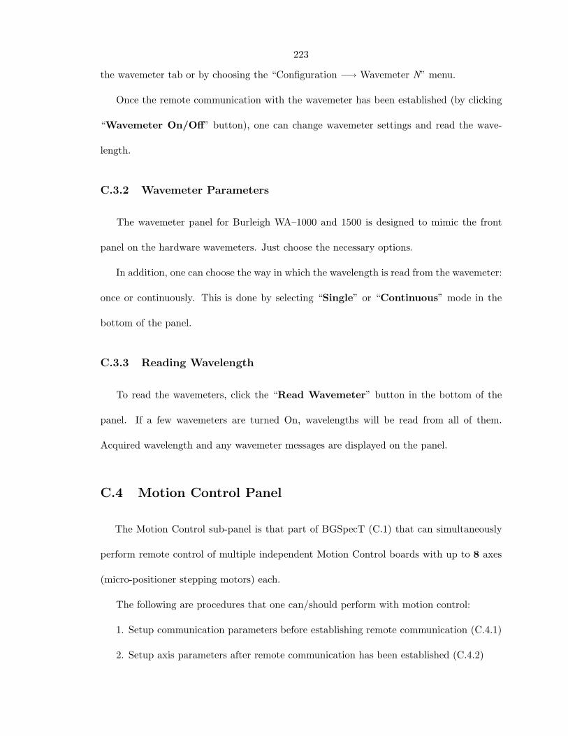
the wavemeter tab or by choosing the “Configuration −→ Wavemeter N” menu.

Once the remote communication with the wavemeter has been established (by clicking

“Wavemeter On/Off” button), one can change wavemeter settings and read the wave-

length.

C.3.2 Wavemeter Parameters

The wavemeter panel for Burleigh WA–1000 and 1500 is designed to mimic the front

panel on the hardware wavemeters. Just choose the necessary options.

In addition, one can choose the way in which the wavelength is read from the wavemeter:

once or continuously. This is done by selecting “Single” or “Continuous” mode in the

bottom of the panel.

C.3.3 Reading Wavelength

To read the wavemeters, click the “Read Wavemeter” button in the bottom of the

panel. If a few wavemeters are turned On, wavelengths will be read from all of them.

Acquired wavelength and any wavemeter messages are displayed on the panel.

C.4 Motion Control Panel

The Motion Control sub-panel is that part of BGSpecT (C.1) that can simultaneously

perform remote control of multiple independent Motion Control boards with up to 8 axes

(micro-positioner stepping motors) each.

The following are procedures that one can/should perform with motion control:


2. Setup axis parameters after remote communication has been established (C.4.2)

224

3. Move axes (C.4.3)

4. Positions file (C.4.4)


To prepare the panel and start communication with the Motion Control board(s), one

first needs to perform some setup through the “Configuration” menu. Please follow the

general instructions on how to setup device communications (C.11), substituting the word

Device with Motion Control where applicable.

Supported Motion Control boards are:

225

• Precision MicroControl:

– DC2-PC100, DCX-PC100, DCX-AT100, DCX-AT200, DCX-AT300 series ISA cards

– DCX-PCI100, DCX-PCI300, MFX-PCI1000 series PCI cards

If a few motion control boards have been selected, one can switch between them either

by clicking the Motion Control tab (one on the very top) or by choosing the “Configuration

−→ Motion Control N” menu.

Once the remote communication with the motion control board has been established

(by clicking “MC Board On/Off” button), one can change axes settings and move axes.

If the computer has been restarted, the board will not remember its axis positions. You

will be prompted to confirm those when turning the board On for the first time.

C.4.2 Motion Axes Parameters

The left half of the panel is for monitoring purposes, and is where the axis position and

status are displayed. Note, the Current and Target positions will be different when the

axis is moving.

Switching between different axes is done through the tabs in the middle of the panel.

The active axis tab will be right against the corresponding axis status and positions row.

Motion axes can be turned On/Off by clicking the “On/Off” button in the bottom of

the axis panel.

It is possible to assign a name to an axis, which is handy when having to deal with too

many of them.

Assigning the value (in motor counts) for the current axis position can be done by

clicking the “Zero” or “Set To” buttons. The former will set the axis position to “0”. The

226

latter will set it to the value typed in the Distance box. You will be asked to confirm the

new axis position assignment.

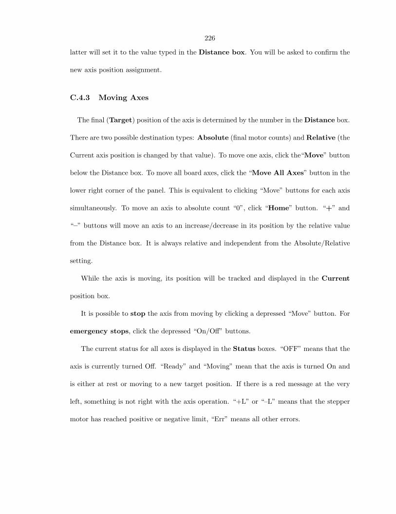
C.4.3 Moving Axes

The final (Target) position of the axis is determined by the number in the Distance box.

There are two possible destination types: Absolute (final motor counts) and Relative (the

Current axis position is changed by that value). To move one axis, click the“Move” button

below the Distance box. To move all board axes, click the “Move All Axes” button in the

lower right corner of the panel. This is equivalent to clicking “Move” buttons for each axis

simultaneously. To move an axis to absolute count “0”, click “Home” button. “+” and

“–” buttons will move an axis to an increase/decrease in its position by the relative value

from the Distance box. It is always relative and independent from the Absolute/Relative

setting.

While the axis is moving, its position will be tracked and displayed in the Current

position box.

It is possible to stop the axis from moving by clicking a depressed “Move” button. For

emergency stops, click the depressed “On/Off” buttons.

The current status for all axes is displayed in the Status boxes. “OFF” means that the

axis is currently turned Off. “Ready” and “Moving” mean that the axis is turned On and

is either at rest or moving to a new target position. If there is a red message at the very

left, something is not right with the axis operation. “+L” or “–L” means that the stepper

motor has reached positive or negative limit, “Err” means all other errors.

227

C.4.4 Positions File

If the position of any axis has been changed, positions for all axes will be saved in the

Configs directory in a file with the name:

“MC”+“ t”+BoardType+“ a”+BoardAddress+“.mc1”.

As new backups are made, the extensions for the previous two backups become “.mc2”

and “.mc3”. These files are created to remember last axes positions between program

startups and computer crashes. The latter two files are saved in case the first one becomes

corrupt.

C.5 Oscilloscope Panel

The Oscilloscope sub-panel can simultaneously and remotely control multiple independent

oscilloscopes with a total number of channels up to double the number of oscilloscopes. Due

to the large number of supported scope models (over 100), this software does not control all

possible scope functions, but rather, accesses major common features to acquire waveforms.

All waveform manipulations (math, etc) are performed on the PC during post-processing.

The following are procedures that one can/should perform with the scopes:


2. Setup scope parameters after remote communication has been established (C.5.3)

3. Acquire and manipulate waveforms (C.5.2)


To prepare the panel and start communication with the oscilloscope(s), one first needs to



228

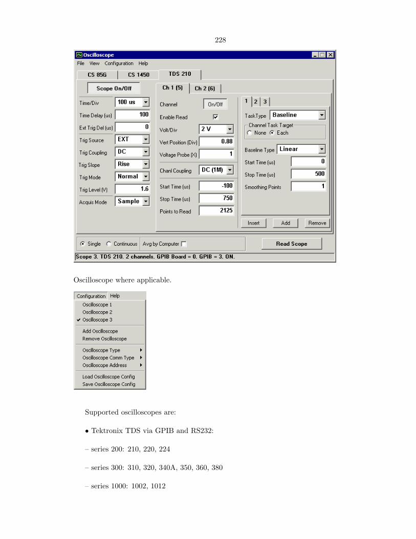
Oscilloscope where applicable.

Supported oscilloscopes are:

• Tektronix TDS via GPIB and RS232:

– series 200: 210, 220, 224

– series 300: 310, 320, 340A, 350, 360, 380

– series 1000: 1002, 1012

229

– series 2000: 2002, 2012, 2014, 2022, 2024

– series 3000: 3012, 3012B, 3014, 3014B, 3032, 3032B, 3034, 3034B, 3052, 3052B, 3054,

3054B

• Tektronix TDS via GPIB:

– series 400: 410, 410A, 420, 420A, 430, 460, 460A

– series 500: 510A, 520A, 520B, 520C, 520D, 524A, 540A, 540B, 540C, 540D, 544A,

580C, 580D

– series 600: 620A, 620B, 620C, 640A, 644A, 644B, 654C, 680B, 680C, 684A, 684B,

684C, 694C

– series 700: 714D, 714L, 724A, 724C, 724D, 744A, 754A, 754C, 754D, 782A, 784A,

784C, 784D, 794D

– series 5000: 5032, 5032B, 5034, 5034B, 5052, 5052B, 5054, 5054B, 5054BE, 5104,

5104B

– series 6000: 6404, 6504, 6604

– series 7000: 7054, 7104, 7154, 7154B, 7254, 7254B, 7304, 7404, 7404B, 7704B

• Tektronix THS via RS232:

– series 700: 710, 710A, 720, 720A, 720P, 730A

• GaGe CompuScope PC plug-in cards (PCI, CompactPCI or ISA):

– 85G, 82G, 8500, 12100, 1250, 1220, 14200, 14100, 1450, 1610, 1602, (6012/PCI) via

PCI

– 85GC, 82GC, 14100C, 1610C via CompactPCI

– (8012, 6012, 1012, 512, 2125, 250, 225, LITE via ISA)

• LeCroy 9400A via GPIB and RS232

If a few scopes have been selected, one can switch between them, either by clicking the

230

scope tab (the one on the very top) or by choosing the “Configuration −→ Scope N” menu.

Once remote communication with the scope has been established (by clicking “Scope

On/Off” button), one can change scope settings and acquire waveforms.

When turning On remote communication with the scope, the current scope configuration

will be retrieved from the scope for GPIB and RS232 scopes. For GaGe CompuScopes, the

last used configuration will be restored.

C.5.2 Waveform Acquisition and Manipulation

1. Read

2. View

3. Save

C.5.2.1 Reading Waveforms

To acquire waveforms on the scope and transfer them to the PC, one just needs to click the

“Read Scope” button in the lower right corner of the Oscilloscope panel. It becomes active

if at least one scope channel is turned On. When multiple scopes are On, their channels

are considered by the software as channels of one scope. When acquiring waveforms, all

scopes are reset to be triggered at the same time. In case of multiple acquisitions (while

“Averaging by Computer” or in “Continuous” mode), scopes are not re-triggered again until

all waveforms are transferred to the PC.

Once the waveforms are acquired, they are put through post-processing procedures that

are defined for each channel individually under Channel Task tabs.

231

C.5.2.2 Viewing Waveforms

All new waveforms are displayed in the Oscilloscope Screen panel. One can access it

through the “View −→ Scope Screen” menu.

Here, each channel has its own horizontal scale - waveform start/stop times define record

limits and the whole record fits into the screen window. One can view time and voltage

values for each channel by moving the mouse over the channel traces. These values will be

displayed right below the screen part, as well as in a tool tip. There are no time/voltage

grids on this panel because each channel may have its own scales.

Channel numbers on the labels are the same as numbers in parenthesis in the channel

tabs on the Oscilloscope panel. One can change a default color for the channel by double-

232

clicking the channel label in the bottom of the scope screen. A single click on the channel

label will bring the trace for that channel on top of others.

If the Oscilloscope Screen panel is closed and reopened, the traces will still be displayed.

However, if one clears waveform traces by double clicking on the black area, they will no

longer be available. One would have to acquire new traces. The same thing happens if one

changes scope or channel critical parameters (time scale, delay time, channel voltage scale,

start/stop times, etc.).

The “Read Scope” button on the bottom of the Oscilloscope Screen window performs

the same function as the same button in Oscilloscope panel and was put there for user

convenience.

Right-clicking the mouse on the screen (black area) will bring up the menu that will

allow the user to save channel waveforms into data files (same as described below). Selecting

“Clear” from this menu (same as double-clicking on the screen) will remove waveform traces

from the screen. Those traces will not be re-displayed until new traces are acquired.

C.5.2.3 Saving Waveforms

If needed, the waveforms can be saved into data files by selecting the “File −→ Save”

or “File −→ Save As” menus in Oscilloscope panel. The “Save As” menu will prompt for

file names for each channel. The “Save” menu will save files with automatically generated

names into the current scope directory. This directory may be changed through the “File

−→ Set Directory” menu. If one needs to save waveforms repeatedly, it is advised to use

the Autosave option under Channel Tasks.

233

Depending on whether the box “Time in Time/Div Units” is checked or not, time will

be saved either in Time/Div units or in seconds. That value in the checkbox is also used

when saving files automatically – via the “File −→ Save” menu, Autosave channel task or

via the “Other −→ Dump Raw Data to File” menu in Spectrum Scan panel (C.8).

Each saved file will have two columns separated by a Tab symbol. The first column is

time and the second column is voltage value in volts.

C.5.3 Oscilloscope Parameters Setup

The oscilloscope panel options span over:

1. Panel (all scopes) – software acquisition and averaging modes

2. One scope (all scope channels) – time scale, delay, triggering and scope acquisition

234

options

3. One scope channel – voltage scale, vertical position, coupling, start/stop times

4. Channel tasks – waveform post processing (baseline, smooth, autosave, voltage dy-

namic range)

One can also Save and Load such oscilloscope configurations to and from a file.

C.5.3.1 Panel Parameters

Panel-wide parameters are software acquisition and averaging modes. Acquisition mode

can be “Single” or “Continuous” (see the bottom of the Oscilloscope panel). In “Single”

mode, the waveforms are acquired only once, which is the same as “Single” triggering

mode on stand alone oscilloscopes. In “Continuous” mode, the waveforms are acquired

until “Read Scope” button is pressed again, which is similar to “Normal” triggering mode

on stand alone oscilloscopes. The reason for having it this way is to make one software

oscilloscope out of a few hardware units.

For averaging, there is a possibility of “Averaging by Computer” for acquired wave-

forms. When this option is enabled, the waveforms are acquired by scopes according to their

acquisition mode settings and then are transferred to a PC and averaged by the software.

This permits higher levels of synchronization and some post processing before the traces

are averaged.

C.5.3.2 Common Scope Parameters

For each scope that is turned ON, one can change a few sets of parameters common to

the whole scope:

235

1. Time scale and trigger delays

2. Triggering options

3. Acquisition options

All of these are located on the left side of the Oscilloscope panel.

For stand alone hardware oscilloscopes, one can select Time/Division, which is the

same as Time/Div or the Horizontal scale on the scope. For GaGe scopes, this will be

replaced by the Sampling Rate which is inverse of the time interval between two adjacent

points in the record. If one of the scopes Time/Div values is not standard (not on the

list, but close to another “wrong” value), one should choose that “wrong” setting. The

difference adjustment will be done automatically.

Time Delay is the delay time between the trigger position and the first point on the

oscilloscope screen, which is not necessarily the first point in the data record. It is positive

when the trigger is displayed on the scope screen and negative when the trigger is to the left

of the screen. Note that for Tektronix scopes, when such a delay is set to zero the trigger

point is on the left of the screen and not in the middle. For oscilloscopes with multiple

record lengths, a minimal record length is usually chosen and the delay time is adjusted

accordingly. That is why it may be disabled.

External Trigger Delay is used to offset waveforms to “true zero” times in cases

when the oscilloscope is being triggered by some delayed signal, but the oscilloscope does

not know about the delay.

Currently, the software supports only one trigger (no second/delayed trigger) for a

scope. All triggering is done only from the “Edge” (e.g. the rise/fall front of the waveform).

In the triggering part of the panel, one can change the Trigger Source (one of the

channels, External, etc.), Trigger Coupling (AC, DC), Trigger Slope (Rise, Fall or

236

both), Trigger Mode (Single, Normal, Auto, etc.) and Trigger Level. For GaGe scopes,

the Trigger Mode is replaced by Channel Mode (Single, Dual) which shows how many

scope channels can be used.

When a scope is acquiring waveforms, the Trigger Mode is set to Single. After all

waveforms are transferred to a PC, it is returned to the previous state. For repetitive

waveform acquisitions when data acquisition speed is important, it is advised to switch the

Trigger Mode to Single.

Acquisition Mode switches between Sample, Average, PeakDetect, Envelope, etc.,

when applicable. For some of these modes, such as Average or Envelope, one may be able

to change the Averaging Number. Time to Average is an estimated time that it takes

the scope to finish averaging waveforms after it was reset. A computer will wait that long

before trying to download the averaged waveform. This is used to minimize communication

traffic between the hardware and a PC.

C.5.3.3 Channel Parameters

The user can set up parameters for individual channels. Switching between the channels

is done through the channel tab. The name of the channel tab is the name of the channel on

the scope (Ch 1, Ch A, Aux 1, etc.). The number in parenthesis is the channel number

in the software, and is the number that goes into the channel label in the Oscilloscope

Screen panel. It is also used to identify oscilloscope channels in the Spectrum Scan panel

(C.8). The number of channels on the scope is determined by the software automatically.

If the software runs out of the maximum allowed number of channels (double the maximum

number of devices in the Oscilloscope panel), it may cut off some of the channels that do

not fit in.

237

The “On/Off” button turns the channel On and Off, reflecting all changes on the

hardware as well (it (dis)appears from the hardware scope screen). For GaGe scopes, this

does not change the Channel Mode between Single and Dual. The “Enable Read” check

does not remove the channel trace from the hardware scope screen. When it is unchecked,

the software will not download the waveform to a PC.

One can change a few voltage parameters: Voltage/Division (vertical scale), Ver-

tical Position of the waveform trace and Voltage Probe (when applicable). For GaGe

scopes, Volt/Div will be replaced by Voltage Range – the allowed voltage range for the

chosen scale. The full range is 10 divisions for Tektronix scopes and 8 divisions for LeCroy

9400A. The Volt/Div scale may affect the Trigger Level when using this channel as the

Trigger Source.

Channel Coupling may be AC, DC, or Ground. The number in parenthesis is input

impedance (50 Ohm or 1 MOhm). Channel Coupling may affect allowed Volt/Div scales.

If the oscilloscope is triggered from one of its channels, both Volt/Div and channel coupling

may affect allowed triggering settings.

The entire waveform does not need to be transferred to a PC. It is possible to choose

the time range (Start and Stop times) that will be downloaded, and only points from this

time interval will be plotted in the Oscilloscope Screen panel. Note that the Start/Stop

times are in the same units as Time/Div (s, ms, µs, etc.). From the Start/Stop times, the

software will calculate the number of Points to Read which cannot be changed and is

there for information purposes only. Depending on these times, the minimum record length

and delay times may be adjusted accordingly. For the LeCroy 9400A, one can Read 1

Point Out of N - each Nth point of the record. This approach can be useful when the

signal on one channel does not need to have as high a time resolution as another.

238

C.5.3.4 Channel Task Parameters

On the right side of the channel panel, one can define Channel Tasks - a set of

manipulations to be done with the acquired waveform. One can change their number by

clicking “Insert”, “Add” and “Remove” buttons. There are a few types of channel tasks:

1. None – default value

2. Dynamic Range

3. Baseline

4. Autosave

5. Smooth

6. Scale Up/Down

All Start/Stop times must be within the selected time range for the channel.

Channel tasks can be applied in several ways: None (same as choosing None task), Each

(applied to each downloaded waveform), Avg (when Averaging by Computer, applied to the

averaged waveform only, not the individual ones), and All (same as Each and Avg together).

All tasks are performed in the order of their appearance and according to their selected

time range.

Dynamic Range is the difference between the minimum 5% and maximum 5% points

of the waveform in a selected time range. This difference is expressed in % of the whole

voltage dynamic range at the selected Volt/Div scale. If the Dynamic Range value does

not fit into the Minimum/Maximum brackets, all waveforms from this acquisition will

be discarded and the acquisition will start again. This task may be very useful when trying

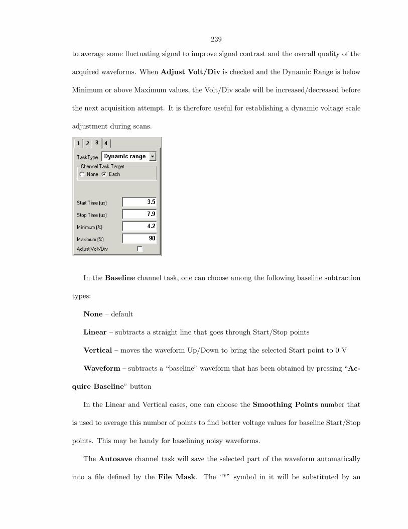
239

to average some fluctuating signal to improve signal contrast and the overall quality of the

acquired waveforms. When Adjust Volt/Div is checked and the Dynamic Range is below

Minimum or above Maximum values, the Volt/Div scale will be increased/decreased before

the next acquisition attempt. It is therefore useful for establishing a dynamic voltage scale

adjustment during scans.

In the Baseline channel task, one can choose among the following baseline subtraction

types:

None – default

Linear – subtracts a straight line that goes through Start/Stop points

Vertical – moves the waveform Up/Down to bring the selected Start point to 0 V

Waveform – subtracts a “baseline” waveform that has been obtained by pressing “Ac-

quire Baseline” button

In the Linear and Vertical cases, one can choose the Smoothing Points number that

is used to average this number of points to find better voltage values for baseline Start/Stop

points. This may be handy for baselining noisy waveforms.

The Autosave channel task will save the selected part of the waveform automatically

into a file defined by the File Mask. The “*” symbol in it will be substituted by an

240

increasing integer number.

The Smooth task will average the waveform over a Smoothing Points window with

a “moving box” method.

The Scale Up/Down channel task scales the waveform vertically via multiplying it by

the Scale Factor. Negative numbers can be used to invert the waveform.

C.5.3.5 Save and Load Configuration

All of the above scope-specific settings may be saved to a file or loaded from a file. To

do that, choose the “Configuration −→ Save/Load Oscilloscope Config” menu. You will be

prompted for a file name.

241

C.6 Delay Generator Panel

The Delay Generator sub-panel is part of BGSpecT (C.1) that can simultaneously

perform remote control of multiple independent delay generators.

The following are procedures that one can/should perform with the delay generators:


2. Setup delay generator parameters after remote communication has been established

(C.6.2)

3. Visualize output pulses (C.6.3)


To prepare the panel and start communication with delay generator(s), one first needs to



242

Delay Generator where applicable.

Supported delay generators are:

• Stanford Research Systems (SRS) DG535 (via GPIB)

If a few delay generators have been selected, one can switch between them either by

clicking the delay generator tab (that at the very top) or by choosing the “Configuration

−→ Delay Generator N” menu.

Once remote communication with the delay generator has been established (by clicking

“DelGen On/Off” button), one can change delay generator settings and adjust delays.

Caution! When remote communication is established with the SRS DG535, all device

parameters are set to factory default settings. It is advised to store delay generator settings

in the device’s memory before clicking the “DelGen On/Off” button.

C.6.2 Delay Generator Parameters

It is possible to change the following values:

1. Trigger parameters

2. Output line parameters

243

3. Delay line parameters

4. Save and Load above settings

C.6.2.1 Trigger Parameters

The trigger part of the panel (at the bottom) is responsible for the delay generator

triggering mode parameters. Triggering mode is selected from the Source list. There are

four different modes for the SRS DG535:

1. Int – Internal. One can change the repetition rate.

2. Ext – External (via Ext input). One can set the threshold voltage, slope and input

impedance.

3. Ss – Single Shot. Triggering is performed by clicking the “Single Shot” button.

4. Bur – Burst mode. It is possible to change the burst rate, number of burst pulses

and their periods.

C.6.2.2 Output Line Parameters

There are 7 output lines that can be configured in the SRS DG535: T0, A, B, ±AB,

C, D, ±CD. They are selected from the Line list. For each, one can change the mode

244

(TTL, NIM, ECL and VAR), load impedance, and polarity (except ±AB and ±CD). In

the Variable mode, it is possible to change the amplitude and offset voltages.

C.6.2.3 Delay Line Parameters

For the SRS DG535 delay generator, the number of delay lines (A, B, C and D) is

different from the number of output lines mentioned above. For each delay line, one can

change the delay time by changing the number in the Relative delay box. The reference

line for a delay line may be selected from the “Line” list. The format of the Relative delay

line will then be as follows:

Delay line name = Delay Generator N + Reference line name + Relative delay time (in

seconds)

The absolute delay time will be displayed in the Absolute Delay box and cannot be

changed by typing in that box.

When there are a few delay generators controlled by the software and one of them

controls the others through external triggering, it is possible to synchronize delay lines

from different devices by checking the “Slaved To Line” box. Prior to that the following

must be done:

1. Click on T0 delay line.

2. From the Slave DelGel list, choose the number of the master device that triggers

the current device.

3. In the Slave Line, choose the delay line on the master device. It must be this line

that triggers the current device.

245

4. Type the delay in the Slave delay box. This is the delay generator’s lag time

between the External and T0 pulses. It is not zero.

5. Click “Slaved To Line” box.

6. Perform same operations for the desired line, choosing the desired slave delay time.

Now the Absolute Delay will be shown with respect to the T0 line of the master delay

generator. Changing the relative delay time for the master delay line will automatically

change delay for the slave delay line.

C.6.2.4 Save and Load Settings

All the device-specific settings described above may be saved to a file or loaded from a

file. To do this, choose the “Configuration −→ Save/Load Delay Generator Config” menu.

You will be prompted for a file name.

For the SRS DG535, it is possible to Store and Recall delay generator settings in devices

designated memory locations 1 – 9 by clicking the “Store” and “Recall” buttons. The

“Clear” button will set all device parameters to their factory default values.

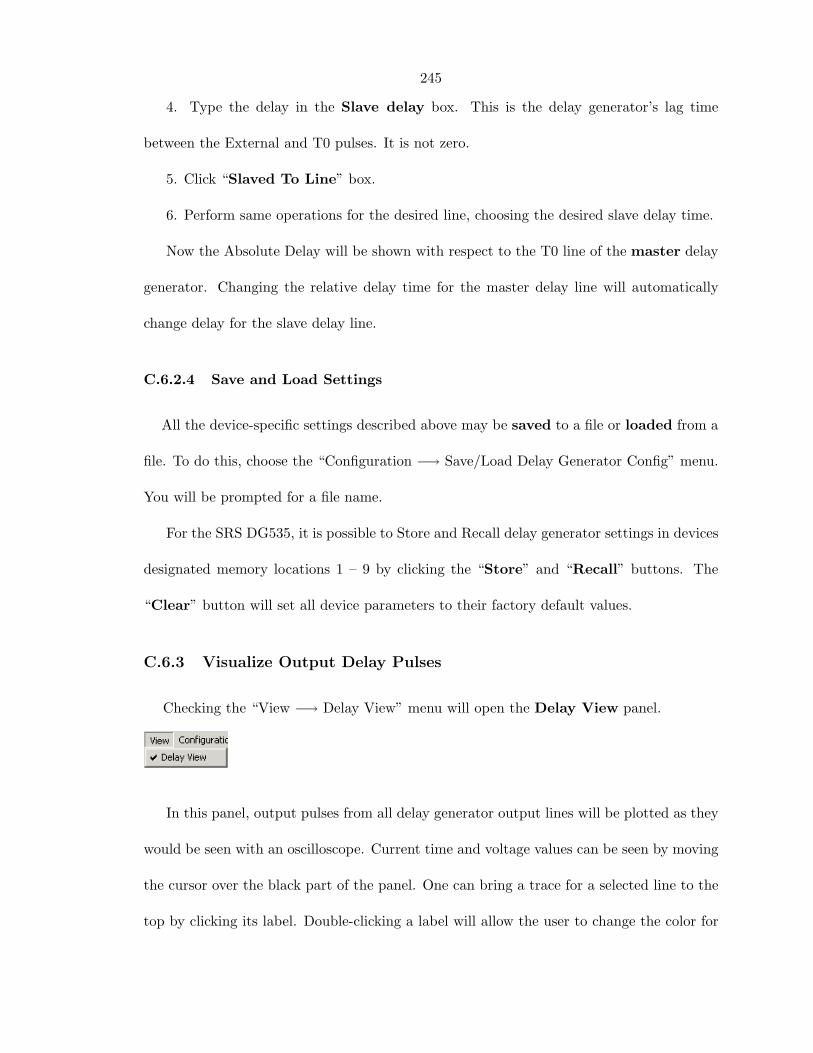
C.6.3 Visualize Output Delay Pulses

Checking the “View −→ Delay View” menu will open the Delay View panel.

In this panel, output pulses from all delay generator output lines will be plotted as they

would be seen with an oscilloscope. Current time and voltage values can be seen by moving

the cursor over the black part of the panel. One can bring a trace for a selected line to the

top by clicking its label. Double-clicking a label will allow the user to change the color for

246

that line. The label name is a combination of the device number in the Delay Generator

panel and the output line name.

C.7 Photon Counter Panel

The Photon Counter sub-panel is the part of BGSpecT (C.1) that can simultaneously

remotely control multiple independent photon counters.

The following are procedures that one can/should perform with the photon counters:


2. Setup photon counter parameters after remote communication has been established

(C.7.2)

3. Read counts (C.7.3)

247


To prepare the panel and start communication with photon counter(s), one first needs to



Photon Counter where applicable.

Supported photon counters are:

• Stanford Research Systems (SRS) SR400 (via GPIB and RS232)

248

If a few photon counters have been selected, one can switch between them either by

clicking the photon counter tab or by choosing the “Configuration −→ Photon Counter N”

menu.

Once remote communication with the photon counter has been established (by clicking

“PhCount On/Off” button), one can change photon counter settings and read counts.

C.7.2 Photon Counter Parameters

Photon Counter panel options span over:

1. Panel (all photon counters) – software acquisition and averaging modes

2. One photon counter (all device counter channels) – counting and display modes,

triggering options, output ports

3. One counter channel – counter input, discriminator and gate options

One can also Save and Load a photon counter configuration to and from a file.

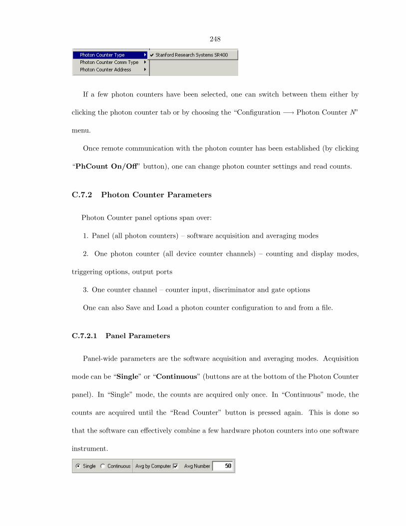
C.7.2.1 Panel Parameters

Panel-wide parameters are the software acquisition and averaging modes. Acquisition

mode can be “Single” or “Continuous” (buttons are at the bottom of the Photon Counter

panel). In “Single” mode, the counts are acquired only once. In “Continuous” mode, the

counts are acquired until the “Read Counter” button is pressed again. This is done so

that the software can effectively combine a few hardware photon counters into one software

instrument.

249

For averaging, there is the option of “Averaging by Computer” for acquired counts.

When this option is enabled, the counts are acquired by photon counters according to their

settings and are then transferred to a PC and averaged by the software.

C.7.2.2 Common Photon Counter Parameters

Count Mode determines how the counting is performed (A,B, A–B, A+B for T preset,

A for B preset). Count Periods determines the number of times the counters perform

their job. The counts from each of these periods are then averaged into one number. That

is why, sometimes, the final number of counts contains extra digits after the decimal point.

If, in addition, the Averaging by Computer is performed, the data will be averaged twice.

Dwell Time is the counter inactive time between two count periods.

D/A Source (A, B, A-B, A+B) and D/A Range (Log or Linear) set the front panel

D/A output source and the scale range for it.

Trigger Slope (Rise or Fall) and Trigger Level determine these parameters for the

external trigger input.

Display Mode switches between Continuous and Hold modes.

Output Port parameters determine the properties of Port1 and Port2 outputs on the

back panel of the SRS SR400. For each Port, one can choose Mode (Fixed or Scan) and

Level. In the Scan mode, Scan Step may be changed.

C.7.2.3 Counter Channel Parameters

The user can set up parameters for individual counter channels. Switching between the

counters is done through the channel tab. The name of the channel tab is the name of

the channel on the device (A, B, T). The number in parenthesis is the absolute channel

250

number in the software, and is used to identify counter channels in the Spectrum Scan

panel (C.8). The number of channels on the photon counter is determined by the software

automatically. If the software runs out of the maximum allowed number of channels (double

the maximum number of devices in the Photon Counter panel), it may cut off some of the

channels that do not fit.

The “Enable Read” check enables/disables downloading counts data from a photon

counter to a PC.

Counter Input selects among allowed input channels for each counter (10 MHz, Input

1, Input 2, External Trigger). For a preset counter (usually T, but may be B in A for B

preset count mode), one can change the counter preset maximum number (in 10 MHz clock

cycles). If this number is reached during the counting, the experiment is ceased.

For each counter Discriminator, it is possible to change the Discriminator Mode

(Fixed or Scan), Discriminator Slope (Rise or Fall) and Discriminator Level. In the

Scan mode, Scan Step will also be available.

For counters A and B, one can select Gate parameters: Gate Mode (CW, Fixed or

Scan), Gate Width and Gate Delay. In Scan mode, Scan Step will also be available.

C.7.2.4 Save and Load Settings

All of the above device-specific settings may be saved to a file or loaded from a file.

To do this, choose the “Configuration −→ Save/Load Photon Counter Config” menu. You

will be prompted for a file name.

For the SRS SR400, it is possible to Store and Recall photon counter settings in devices

designated memory locations 1 – 9 by clicking the “Store” and “Recall” buttons. The

“Clear” button will set all device parameters to their factory default values.

251

C.7.3 Reading Counts

To read photon counter counts, click the “Read Counter” button in the bottom of

the panel. If a few photon counters are turned On, counts will be read from all of them.

Acquired counts are displayed at the top of the panel.

C.8 Spectrum Scan Panel

The Spectrum Scan sub-panel is part of BGSpecT (C.1) that uses instrument panels

to record spectra. This powerful tool has many fine tuning settings that allow he user to

perform more efficient and fast scans. It requires some time to set up, but then the scan

can be completely automated and does not require human intervention.

To perform a successful scan, the following needs to be done:

252

1. Decide on your sources and detectors (C.8.1)

2. Setup sources (C.8.2)

3. Setup detectors (C.8.3)

4. Use Spectrum View (C.8.4)

5. Setup other features (C.8.5)

6. Perform the actual scan (C.8.6)

C.8.1 Sources and Detectors

In Spectrum Scan, the instruments are divided into sources and detectors.

Sources are instruments that are used to change some scan parameters such as wave-

length, delay, etc. Hence, devices from Lambda Tune (C.2), Motion Control (C.4) and

Delay Generator (C.6) panels may be used as scan sources. In addition, there is a built-in

four-channel timer in Spectrum Scan that may be used as a source.

Detectors are instruments that are used to record data (e.g., waveforms, wavelengths).

Hence, devices from Oscilloscope (C.5), Wavemeter (C.3) and Photon Counter (C.7) panels

may be used as scan detectors.

It is advised to turn on all necessary source and detector devices using their panels

before starting the Spectrum Scan panel. Doing so may save some confusion about device

availability.

C.8.2 Sources Setup

The sources are located on the left side of the Spectrum Scan panel. The principle of

working with sources is similar to that for devices in instrument panels. To access sources,

one should first go to the “Source” menu and create a sufficient number by clicking the

253

“Source −→ Add Source” and the “Source −→ Remove Source” menus. Switching between

different sources can be done either by clicking on the ‘Sources’ tab or by selecting the

appropriate “Source −→ Source N” menu. The maximum allowed number of sources (up

to 128) can be changed by clicking “Source −→ N Sources Max” menu.

The user should next assign some device to each source. The order in which the sources

are arranged is very important. When recording a spectrum, the sources are scanned in a

nested loop order with the first source on the outermost (that is, the largest) loop and the

last source on the inside (the smallest and therefore the most frequently repeated) loop.

Currently available source devices will be displayed under the “Source” menu. They

will be in the form of menus with the device name and its number in the instrument

panel. Only those devices that have been turned “On” (remote communication successfully

established) will be shown. The Internal Clock will always be displayed, since it is built

into the Spectrum Scan panel. It is possible to refresh the list of currently available source

devices by clicking the “Source −→ Refresh Sources” menu.

To assign sources, first select the desired source and then choose an appropriate source

device. Since many of the source devices have multiple channels, the same device may be

254

assigned to multiple sources, but each channel may be assigned to only one source. Upon

successful assignment, the abbreviated name of the source will be displayed in the source

tab.

After the sources have been assigned, each of them should be configured. First, a

channel to scan should be selected for a source. For a lambda tune source, it will be a

“Tune source” list; for a delay generator, “Delay Line”; for Motion Control, “MC Axis”;

and for Internal Clock, “Clock Channel”. Only unassigned channels are displayed in this

list.

In the case of the wavelength, the user can choose between nanometers and wavenum-

bers as units.

Now one should choose the desired Start, Stop and Step for the scan. In the case of

the wavelength, only values within the lambda tune calibration range will be allowed. The

Step Size may be larger than the difference between Stop and Start. In such a cases, only

one source position will be used during the scan – Start.

If the menu “Other −→ Real Time Dark (Baseline)” is checked, one can collect the

baseline signal in “real time.” In this case, at each source position before recording signal

all sources, all except Internal Clocks will be moved to their “Dark” positions, that is

where the signal consists only of noise, some reference value, or is “off-resonance,” etc.

“Dark” signal collection happens inside the most enclosed loop, and so acquiring “dark”

data doubles the scan time.

To configure Real Time Dark, first check the “Real Time Dark from” box. Then

select a source and a channel. Only assigned source devices will be available here, but there

is no limit on channel numbers. After that, type in the desired value for the “dark” position

of that source.

255

If a delay generator was chosen as a scan source, it may be used to trigger the full data

acquisition cycle (all necessary devices) from a computer. To do this, one should enable the

Master Trigger mode by checking the “Other −→ Master Trigger” menu. Then, check

the “Trig Master” box. Only one delay generator can be used for the Master Trigger, and it

must be set to Single Shot triggering mode. The “Trig Rate” is the desired rate of triggering

by computer. This is the maximum value. In case the whole data collection is slower than

one triggering period, the actual triggering rate will be smaller. This is done to ensure that

no data are lost.

Source Settle Time is the amount of time between the end of moving the source to a

new position and resetting the detectors to start data acquisition. This provides a waiting

period for the system under study to adjust to the new conditions. In most cases this time

is set to zero.

If for some reason the user does not wish to scan a certain source, it is possible to

disable it for the scan by checking the “Don’t scan this source” box.

256

C.8.3 Detectors Setup

The detectors are located on the right side of the Spectrum Scan panel. The principle

of working with detectors is similar to that used for sources. To access detectors, one

should first go to the “Detector” menu and make enough boxes by clicking the “Detector

−→ Add Detector” and the “Detector −→ Remove Detector” menus. Switching between

different detectors can be done either by clicking on the ‘Detectors’ tab or by selecting the

appropriate “Detector −→ Detector N” menu. The maximum allowed number of detectors

(up to 128) can be changed by clicking the “Detector −→ N Detectors Max” menu.

Then, detector should be assigned to a device. Currently available detector channels

will be displayed under the “Detector” menu. They will be in the form of menus with the

device name in the instrument panel and channel number. Only those device channels that

have been turned “On” (remote communication successfully established) will be displayed.

It is possible to refresh the list of currently available detector channels by clicking the

“Detector −→ Refresh Detectors” menu.

To assign detectors, first select the desired detector and then choose an appropriate

257

device channel. The same device channel may be assigned to multiple detectors in order to

be able to perform different post-processing mathematics. Upon successful assignment, the

abbreviated name of the detector will be displayed in the detector tab.

After the detectors have been assigned, each of them should be configured. First, an

available measurement type should be selected for a detector. This measurement will be

used to find the final number that will be saved in the spectrum file.

There are a few possible measurement types:

1. Raw Signal – no post-processing is done

This is the only type available for the wavemeter and photon counter. For oscilloscopes,

no number will be calculated or saved into the spectrum.

2. Mean – calculates the average value (mean) for all waveform points

3. Peak-to-Peak – finds the difference between the maximum and the minimum in the

waveform

4. Integral – calculates the area under the curve

5. Exponential Decay – calculates the time constant for exponential decay

The user can decide if the original data from detector device should be inverted by

checking “Inverted Signal” box. The “Power/Energy” meter box can be checked to indicate

that the current detector is measuring something like laser power or pulse energy. This

value might be used to normalize data from other detectors, for example.

In Integral measurements, one should make there are an appropriate number of “peaks”

258

– that is, ranges for curve integration. This is done by clicking the “Add” and “Remove”

buttons in the bottom of the detector panel. Each of the peaks will then need Min/Max

times assigned as well as the peak name.

In the case of an oscilloscope channel as a detector, one should choose the desired

Minimum and Maximum times. They will determine the time interval over which to

post-process the measurement. Smoothing Points are used in case there is a need to do

intermediate data smoothing when performing measurement math.

If for some reason, the user does not wish to use a certain detector, it is possible to

disable it for the scan by checking the “Don’t use this detector” box.

C.8.4 Spectrum View

Acquired spectra can be viewed in the Spectrum View panel, accessed via the “View −→

Spectrum View” menu.

In order to view spectral plots (traces) in Spectrum View, all parameters in that panel

must be set before the beginning of the scan.

259

To add and remove traces, use the “+” and “–” buttons. Switching between different

traces is done by clicking a trace’s label on the right side of the panel. Parameters of that

trace will be displayed in boxes above the plot area.

For each trace, select references for the X and Y axes of the plot. For the X axis, it

may be one of the sources or detectors (if detector is a wavemeter). For the Y axis, only

detectors are allowed. If the measurement type for a detector is Integral, then the Peak

box will appear, offering a selection of the peaks whose area is calculated in this detector

measurement.

Then choose the plot type. It will usually be Data. If Real Time Dark baselining is

enabled for some of the sources, Baseline may also be selected to plot the baseline only or

Data–Bsl for a difference between normal and dark (baseline) data.

It is possible to change the trace color by double-clicking the trace label. Right-click

260

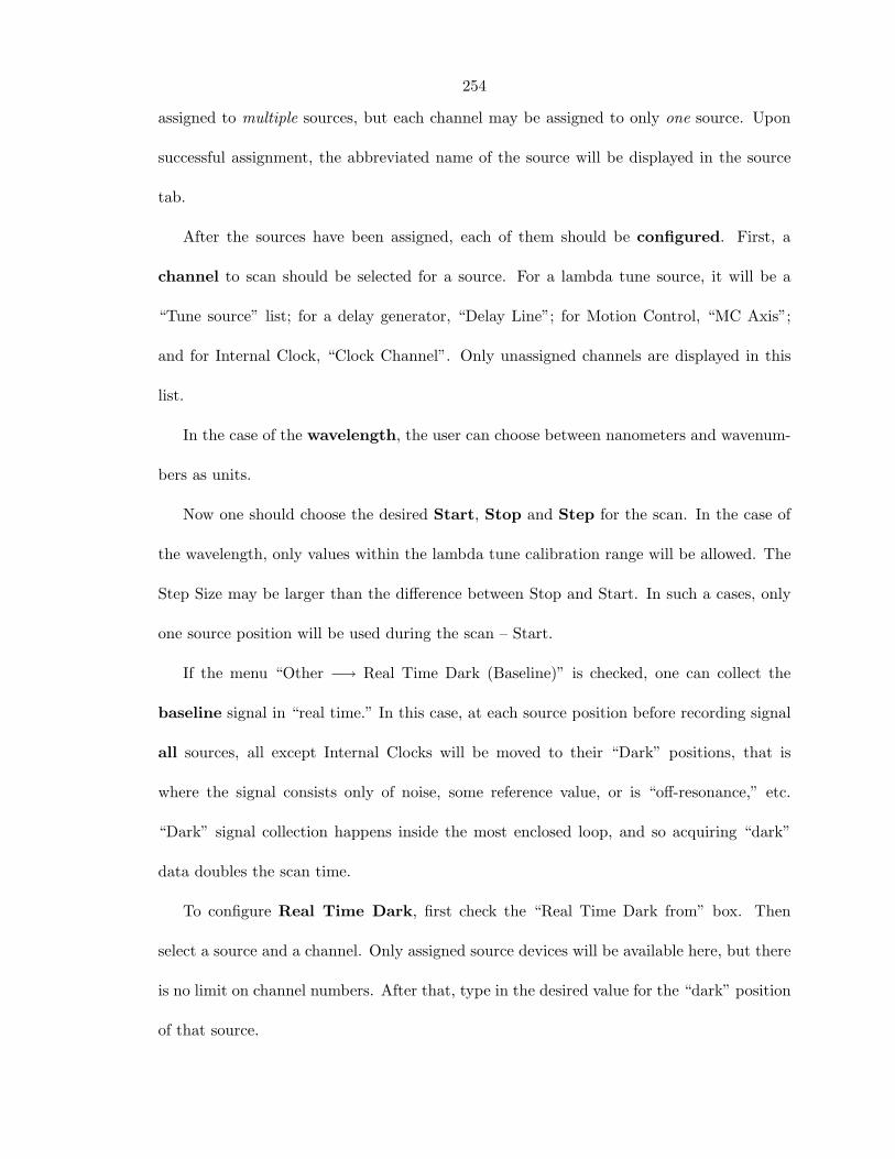
on the label to bring up a menu to choose the trace plotting style: Line or Dots. If Line

is selected, the trace will be plotted as dots connected by lines. If there are a few dots with

the same X and different Y, the average Y will be used to plot a line. This usually occurs

for multi-dimensional scans (when using a few sources).

The scale on the plot is adjusted to fit the screen for each trace as new points are

acquired. To view (X,Y) values, move the mouse over the plot. Current values will be

displayed below the plot and in the tool tip.

C.8.5 Other Features

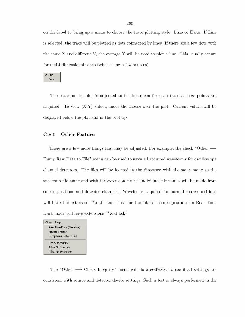
There are a few more things that may be adjusted. For example, the check “Other −→

Dump Raw Data to File” menu can be used to save all acquired waveforms for oscilloscope

channel detectors. The files will be located in the directory with the same name as the

spectrum file name and with the extension “.dir.” Individual file names will be made from

source positions and detector channels. Waveforms acquired for normal source positions

will have the extension “*.dat” and those for the “dark” source positions in Real Time

Dark mode will have extensions “*.dat.bsl.”

The “Other −→ Check Integrity” menu will do a self-test to see if all settings are

consistent with source and detector device settings. Such a test is always performed in the

261

beginning of each scan. If the test has been passed, the “Scan” button will be enabled,

otherwise an error message will be displayed in the bottom of the Spectrum Scan panel. If

you are sure that all settings are correct but you still get an error message in the status

bar, or “Scan” button is disabled, click that menu to perform the integrity test again.

Usually, if there were no sources or detectors assigned, the integrity test will not allow

the scan to be conducted. To override that, the user can check either the “Other −→ Allow

No Sources” or “Other −→ Allow No Detectors” menus.

The “Number of acquisitions” button under the source panel determines how many

times detector readings are performed at each source position. They are performed one

after another at all source positions fixed (inside the most frequent source loop).

The file name to store the scan results may be chosen under the number of acquisitions.

If a file with that name already exists, it will not be overwritten. Instead, another file with

the same name and prefix “N ” will be created, where N is a positive number (1, 2, ...).

The directory for the scan file may be changed by clicking the “File −→ Set Spectrum

Directory” menu.

One can Save and Load the above settings into a series of files by clicking the “File −→

Save Scan Configuration As” and “File −→ Load Scan Configuration” menus. When the

scan configuration is being loaded, the software will try to establish remote communication

with all necessary devices if it has not been done.

Note that when using the delay generator as a source, its parameters are stored in and

recalled from its memory location 9 and is therefore reserved.

If a few scans are to be performed without human intervention, it is possible to place

a few scan jobs in a queue by clicking the “File −→ Add to Job List” menu. The list

of such queued jobs may be purged by clicking the “File −→ Clear Job List” menu. The

262

scan jobs from this list are transferrable between program sessions. The list is not purged

upon completion of all jobs in it. This should be done manually by clicking the “File −→

Clear Job List” menu.

Panel settings can be Saved and Loaded via the “File −→ Save Panel Configuration As”

and “File −→ Load Panel Configuration” menus.

C.8.6 Performing the Scan

If everything was configured properly, the “Scan” button will be enabled. Click it to

start the scan. If the scan needs to be aborted, click the “Scan” button again. This may

be done both during the scan and when it was paused.

If there are any scan jobs queued in a job list, the “Scan Jobs” button will be enabled.

By clicking it, one can perform scans from the list. In the case where no prior panel setup is

required, scan job configurations will be loaded automatically and scans will be performed

in the order of their appearance in the list. Pre-scan panel settings will be discarded if they

were not added to the job list.

Clicking the “Scan Jobs” button again will abort all scans in the queue. Clicking the

“Scan” button will stop only the current scan job. If there are more scans to be done, the

program will proceed with them.

The scan may be paused by clicking the “Pause” button. This will not allow the user

263

to change scan parameters; however, it would be possible to adjust device parameters at

their owner panels. To resume the scan, click the “Pause” button again. Please note that

pausing the scan does not halt all operations immediately. Waiting to resume the scan is

done after the current detector read cycle is finished.

The scan results are saved as lines with numbers separated by the tab symbol. The very

first line of the file will have source and detector names for easier data identification. At the

same time, selected traces are displayed in a Spectrum View (C.8.4) window (if opened).

The acquired data are added to the scan file. If something unexpected happens (com-

puter or equipment crash), the data should not be lost.

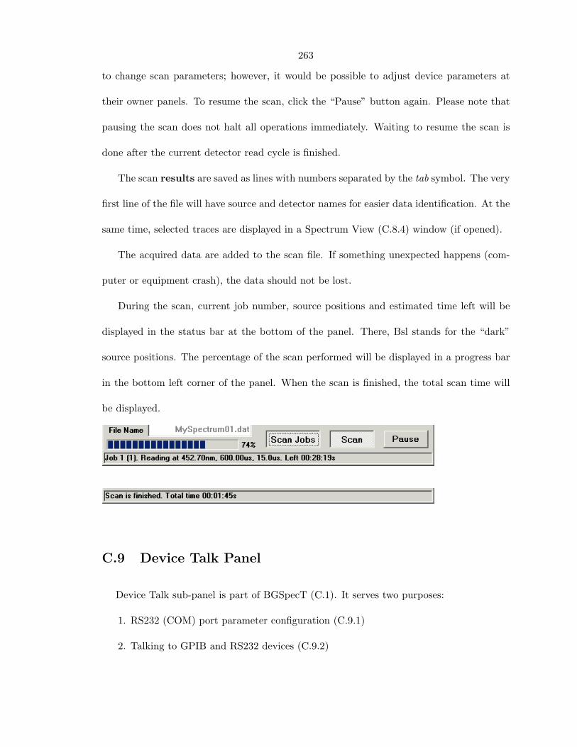
During the scan, current job number, source positions and estimated time left will be

displayed in the status bar at the bottom of the panel. There, Bsl stands for the “dark”

source positions. The percentage of the scan performed will be displayed in a progress bar

in the bottom left corner of the panel. When the scan is finished, the total scan time will

be displayed.

C.9 Device Talk Panel

Device Talk sub-panel is part of BGSpecT (C.1). It serves two purposes:

1. RS232 (COM) port parameter configuration (C.9.1)

2. Talking to GPIB and RS232 devices (C.9.2)

264

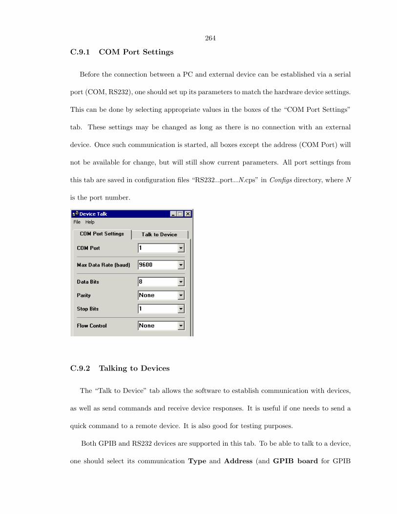
C.9.1 COM Port Settings

Before the connection between a PC and external device can be established via a serial

port (COM, RS232), one should set up its parameters to match the hardware device settings.

This can be done by selecting appropriate values in the boxes of the “COM Port Settings”

tab. These settings may be changed as long as there is no connection with an external

device. Once such communication is started, all boxes except the address (COM Port) will

not be available for change, but will still show current parameters. All port settings from

this tab are saved in configuration files “RS232 port N.cps” in Configs directory, where N

is the port number.

C.9.2 Talking to Devices

The “Talk to Device” tab allows the software to establish communication with devices,

as well as send commands and receive device responses. It is useful if one needs to send a

quick command to a remote device. It is also good for testing purposes.

Both GPIB and RS232 devices are supported in this tab. To be able to talk to a device,

one should select its communication Type and Address (and GPIB board for GPIB

265

devices). In the case where these parameters were assigned to some device in one of the

BGSpecT sub-panels, such information will be displayed.

One can Start/Stop communication with the device by selecting Remote Status. For

assigned devices, this will also turn them On/Off in their owner panels. If an assigned

device is turned On, its Device ID (as stored in the program) will be displayed. If the

devices’ remote status was changed via its owner panel, such information may be renewed

by clicking the “Refresh” button.

It is possible to send a string (command) to a device by clicking the “Write” but-

ton. The response string from the device may be received by clicking the “Read” button.

“Query” will do both Write and Read. The response from the device is displayed in the

window below the buttons.

266

C.10 Devices

Devices are individual pieces of equipment. They usually have the same names as

instruments, although many different devices may be the same kind of instrument. Device

types are:

– Lambda Tune

– Wavemeter

– Motion Control

– Oscilloscope

– Delay Generator

– Photon Counter

C.11 Device Setup

After choosing some Instrument sub-panel from BGSpecT, the panel needs to be setup

before communication takes place. There are some common guidelines on how to do this,

independent of the instrument type.

Each Instrument panel can simultaneously control multiple devices. For example, the

Oscilloscope panel can read waveforms from a few independent digital oscilloscopes without

having to switch between them, i.e., turning one Off and another one On. Each of the

oscilloscopes (or other type of instruments) are referred to as devices (C.10). To setup each

device, one needs to follow a few steps by selecting a number of “Configuration” sub-menus:

1. Create device in the panel (C.11.1)

2. Choose device type (C.11.2)

3. Choose device communication type (C.11.3)

267

4. Choose device communication address (C.11.4)

5. Start communication (C.11.5)

6 (optional). Backup panel configuration (through “File” menu) (C.11.6)

7. Getting help (C.11.7)

C.11.1 Create Device

First, there should be a new device tab created for each device. This is done by

clicking “Configuration −→ Add Device”. Each time another device is created, in addition

to the new tab, a related “Configuration −→ Device N” menu will appear where N is a

number. One can create only a certain maximum number of devices that is specified for

each instrument panel separately.

Switching between different devices is performed by choosing the respective tab or the

“Configuration −→ Device N” menu.

To remove unnecessary device tabs, one can use the “Configuration −→ Remove Device”

menu. Each time it is clicked, it will remove the active (selected) device.

C.11.2 Device Type

Each device should be assigned a type, a communication address, and when applicable,

a communication type.

Usually, each instrument panel supports a few different device types. The device type

268

may be chosen through selecting one of the “Configuration −→ Device Type” sub-menus.

This has to be done even if only one device type is supported by the current software version.

C.11.3 Device Communication Type

In most cases, each device has only one communication type. Physical equipment,

represented by a device, may be either a PC plug-in card (PCI or ISA) or a stand alone

unit with GPIB (IEEE-488.2) or RS232 (COM port on a PC) communication capabilities.

Some stand alone units may have both GPIB and RS232 ports. In this case, if supported

by the current version of software, the user can change that communication type through

the the “Configuration −→ Device Comm Type” sub-menus. Otherwise, an appropriate

menu will be selected automatically. In addition to this, for communication to take place

one may need to carry out some additional steps.

For GPIB devices, a GPIB plug-in card must be installed in the computer along with the

GPIB drivers. Both GPIB and RS232 equipment must be connected to a PC by appropriate

cables. For RS232 devices, appropriate COM port parameters should be adjusted through

the Device Talk (C.9) panel to match the settings on the device itself.

C.11.4 Device Communication Address

Next a communication address should be assigned to the device through one of the

“Configuration −→ Device Address” sub-menus.

In the case of GPIB devices, it is a GPIB address selected on the physical equipment.

It can be a number between 1 and 15. Also, for GPIB devices, one can select what GPIB

269

board the device is connected to by choosing one of the “Configuration −→ Device Address

−→ GPIB N Board” sub-menus.

For RS232 devices, it is an address of a COM port on the PC through which communi-

cation is supposed to occur. Only addresses of installed COM ports are available.

For PC plug-in cards, the address is a card number or index. Usually, the card manu-

facturer will supply configuration software for their cards. In such cases, the device address

is a card number or index in that configuration software. For example, GaGe CompuScope

card numbering starts with 1; if there are 2 cards installed, one of them will have address

1 and another will have address 2. For PMC motion control cards, the numbering starts

with 0.

For devices of the same communication type, the same address may be assigned only

once. If the address needs to be re-assigned to another device, the user should free that

address first by choosing the “Configuration −→ Device Address −→ Clear” menu.

270

C.11.5 Turning Device On/Off

If all the above has been done correctly, the “Device On/Off” button (in the upper

left corner of the panel) will become enabled. To start communication with the physical

equipment, simply press this button. In most cases, the software will read device parameters

from the equipment, i.e., time and voltage scales from the oscilloscope. In other cases,

additional information will need to be supplied, i.e. a calibration file for Lambda Tune.

In some stand alone units, when communication is started the panel with knobs on the

equipment becomes locked and all control is performed through software only. This is why

some functions must be set up manually prior to starting communication, in case they are

not accessible with software. Remember that the actual equipment should have its power

turned on. To gain access to the locked knobs, remote communication must be stopped by

pressing the “Device On/Off” button again.

C.11.6 Panel Configuration Backup

Steps 1 through 4 do not have to be repeated every time the instrument panel is started.

When closing the panel, information about tabs and devices will be saved in the .ini file.

The next time the panel is opened, this information will be retrieved from the file, repeating

steps 1-4, but communication will not be started automatically. Step 5 (C.11.5) should be

done for each device again.

In addition to the .ini file, one can also save the necessary information to, and load it

from, a file through the “File” sub-menus.

271

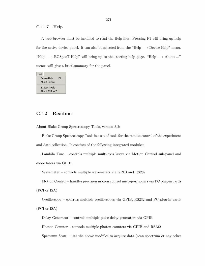
C.11.7 Help

A web browser must be installed to read the Help files. Pressing F1 will bring up help

for the active device panel. It can also be selected from the “Help −→ Device Help” menu.

“Help −→ BGSpecT Help” will bring up to the starting help page. “Help −→ About ...”

menus will give a brief summary for the panel.

C.12 Readme

About Blake Group Spectroscopy Tools, version 3.2:

Blake Group Spectroscopy Tools is a set of tools for the remote control of the experiment

and data collection. It consists of the following integrated modules:

Lambda Tune – controls multiple multi-axis lasers via Motion Control sub-panel and

diode lasers via GPIB

Wavemeter – controls multiple wavemeters via GPIB and RS232

Motion Control – handles precision motion control micropositioners via PC plug-in cards

(PCI or ISA)

Oscilloscope – controls multiple oscilloscopes via GPIB, RS232 and PC plug-in cards

(PCI or ISA)

Delay Generator – controls multiple pulse delay generators via GPIB

Photon Counter – controls multiple photon counters via GPIB and RS232

Spectrum Scan – uses the above modules to acquire data (scan spectrum or any other

272

kind of signal dependence)

Device Talk – configures COM ports and talks to individual GPIB and RS232 devices

Useful features:

– Simultaneously controls multiple devices of the same kind

– Controls devices via GPIB and RS232 interfaces as well as PC plug-in cards (PCI or

ISA)

– Simultaneously controls multiple GPIB boards

– Smart oscilloscope waveform acquisition

– Wavelength source wavelength conversions

– Master/Slave locking of delay lines from pulse/delay generator

– Huge number of supported oscilloscopes

– Easy spectrum acquisition

– Flexible to configure

– User friendly interface. Partial Windows XP themes support

Installation.

To install the program, copy an executable BGSpecT.exe, along with the Help direc-

tory into your destination directory. You will also need to put the files from the sys

directory into your Windows system directory (something like C:\Windows\System or

C:\WINNT\system32 – the one that has many DLL files in it). If you are prompted

to overwrite your existing files, choose No.

To uninstall this software from your system, just delete the executable and all unneces-

sary configuration files. No records are made in Windows registry during installation and

273

subsequent use of the program.

Hardware requirements:

Minimum

– CPU - Pentium or better

– RAM - 16 MB

Comfortable

– CPU - Pentium III, Athlon or better, 500 MHz or better

– RAM - 256 MB or larger

All necessary plug-in cards should be installed with the drivers supplied by the manu-

facturer.

Software requirements:

1. Microsoft Windows 95, 98, ME, NT (3.5+), 2000 or XP

2. Visual Basic 6 runtime files (can be downloaded from the Microsoft website)

3. All necessary drivers for hardware in use, i.e. drivers for GPIB cards (National

Instruments only), GaGe CompuScope drivers (version 3.50 and higher), PMC motion

control drivers (version 1.3 or higher)

All necessary drivers can be obtained from the hardware manufacturers, and must be

installed and properly configured. To communicate with RS232 devices, COM ports should

be physically present and enabled (installed) in Windows.

Known incompatibilities and limitations:

1. Hardware drivers. Sometimes plug-in card manufacturers will stop supporting old

274

hardware in their new driver releases, but the old drivers do not support new hardware.

Precision MicroControl driver version 3.0+ supports only new PCI cards; for old ISA cards,

use driver versions 2.23 and lower. GaGe CompuScope driver version 3.50 supports only

new PCI cards (class CP500); for old ISA and class X012/PCI cards, use driver versions

3.46.02 and lower. However, the older drivers may be incompatible with a currently used

SDK based on the 3.50.00 driver.

2. Some legacy devices support only IEEE-488.1 and not the IEEE-488.2 GPIB stan-

dard. They may be used with only 1 GPIB board in a system. Among currently supported

by this software devices are: LeCroy 9400 oscilloscopes, SRS DG535 delay generators,

Burleigh 1000 and 1500 wavemeters, and SRS SR400 photon counters.

3. When turning Off a GPIB device, some devices do not turn off from remote mode

because of the above. This happens because these GPIB devices require sending a GPIB

command that stops all GPIB communications with all GPIB devices on the bus. Such a

command would also disconnect all other GPIB devices in use, and therefore, is sent only

when turning Off the last device connected to the board.

4. For Tektronix oscilloscopes, extra options are not supported (such as extra memory,

voltage probes, etc.). For GaGe oscilloscopes, some extra options are not supported (such

as master/slave, multiple records).

C.13 License Agreement

Blake Group Spectroscopy Tools (BGSpecT) software, California Institute of Technology.

End-User License Agreement.

PLEASE READ THIS DOCUMENT CAREFULLY BEFORE USING THE ENCLOSED

275

SOFTWARE. THIS AGREEMENT LICENSES THE USE OF THE ENCLOSED SOFT-

WARE TO YOU AND CONTAINS WARRANTY AND LIABILITY DISCLAIMERS. US-

ING ANY PART OF THE SOFTWARE INDICATES THAT YOU ACCEPT THESE

TERMS AND INDICATE YOUR ACCEPTANCE OF THIS LICENSE AGREEMENT

AND WARRANTY. IF YOU DO NOT AGREE TO THE TERMS AND CONDITIONS

OF THIS AGREEMENT, DO NOT USE THE SOFTWARE.

License:

This Agreement allows you to:

(a) Use the BGSpecT software on a single computer or a single System at a time. The

BGSpecT software is licensed only for use on an Approved System.

(b) Make one copy of the BGSpecT software in machine-readable form solely for backup

purposes. You must reproduce on any such copy all copyright notices and any other pro-

prietary legends on the original copy of the BGSpecT software.

Restrictions:

You may not make or distribute any copy of BGSpecT software, or electronically trans-

fer the BGSpecT software from one computer to another, or over a network, or from one

System to another. You may not decompile, reverse engineer, disassemble, or otherwise

reduce the BGSpecT software to a human-perceivable form. You may not modify, rent,

lease, lend, resell for profit, distribute or create derivative works based upon the BGSpecT

software or any part thereof.

Ownership and Distribution:

276

The foregoing license grants you limited rights to use the BGSpecT software. Although

you own the disk or CD-ROM on which the BGSpecT software is recorded, you do not be-

come the owner of, and California Institute of Technology (and its licensors) retains title to,

the BGSpecT software, and all copies thereof, and all associated patent rights, copyrights,

trade secret rights and other intellectual property rights therein and thereto. All rights not

specifically granted in this Agreement are reserved by California Institute of Technology.

Warranty:

The BGSpecT software and information is provided “as is” without warranty of any

kind, either expressed or implied, including but not limited to the implied warranties of

merchantability and/or fitness for a particular purpose. The author takes no responsibility

for any kind of damage caused by the BGSpecT software. Use this program at your own

risk.

Blake Group Spectroscopy Tools Software

Documents

Transcript of Blake Group Spectroscopy Tools Software