BLADE: Filter Learning for General PurposeComputational Photography

Pascal Getreuer, Ignacio Garcia-Dorado, John Isidoro, Sungjoon Choi,Frank Ong, Peyman Milanfar

Google Research, Mountain View CA, USA

December 11, 2017

Abstract The Rapid and Accurate Image Super Resolution (RAISR)method of Romano, Isidoro, and Milanfar is a computationally efficient im-age upscaling method using a trained set of filters. We describe a generaliza-tion of RAISR, which we name Best Linear Adaptive Enhancement (BLADE).This approach is a trainable edge-adaptive filtering framework that is general,simple, computationally efficient, and useful for a wide range of problems incomputational photography. We show applications to operations which mayappear in a camera pipeline including denoising, demosaicing, and stylization.

1 Introduction

In recent years, many works in image processing have been based on nonlocal patch modeling.These include nonlocal means of Buades, Coll, and Morel [3] and the BM3D denoising methodof Dabov et al. [7] and their extensions to other problems including deconvolution [14] anddemosaicing [8,9]. While these methods can achieve state-of-the-art quality, they tend to beprohibitively computationally expensive, limiting their practical use.

Deep learning has also become popular in image processing. These methods can tradequality vs. computation time and memory costs through considered choice of network ar-chitecture. Particularly, quite a few works take inspiration from partial differential equation(PDE) techniques and closely-connected areas of variational models, Markov random fields,and maximum a posteriori estimation. Roth and Black’s fields of experts [22], among othermethods [24, 25, 34], develops forms of penalty functions (image priors) that are trainable.Schmidt and Roth’s cascade of shrinkage fields [25] and Chen and Pock’s trainable non-linear reaction diffusion [5] are designed as unrolled versions of variational optimizationmethods, with each gradient descent step or PDE diffusion step interpreted as a network

1

arX

iv:1

711.

1070

0v2

[cs

.CV

] 7

Dec

201

7

layer, then substituting portions of these steps with trainable variables. These hybrid deeplearning/energy optimization approaches achieve impressive results with reduced computa-tion cost and number of parameters compared to more generic structures like multilayerconvolutional networks [5].

Deep networks are hard to analyze, however, which makes failures challenging to diagnoseand fix. Despite efforts to understand their properties [1, 15, 18, 29], the representationsdeep networks learn and what makes them effective remain powerful but without a com-plete mathematical analysis. Additionally, the cost of running inference for deep networksis nontrivial or infeasible for some applications on mobile devices. Smartphones lack thecomputation power to do much processing in a timely fashion at full-resolution on the pho-tographs they capture (often +10-megapixel resolution as of 2017). The difficulties are evenworse for on-device video processing.

These problems motivate us to take a lightweight, yet effective approach that is trainablebut still computationally simple and interpretable. We describe an approach that extendsthe Rapid and Accurate Image Super Resolution (RAISR) image upscaling method of Ro-mano, Isidoro, and Milanfar [21] and others [6, 13] to a generic method for trainable imageprocessing, interpreting it as a local version of optimal linear estimation. Our approach canbe seen as a shallow two-layer network, where the first layer is predetermined and the secondlayer is trained. We show that this simple network structure allows for inference that iscomputationally efficient, easy to train, interpret, and sufficiently flexible to perform well ona wide range of tasks.

1.1 Related work

RAISR image upscaling [21] begins by computing the 2 × 2 image structure tensor on theinput low-resolution image. Then for each output pixel location, features derived from thestructure tensor are used to select a linear filter from a set of a few thousand trained filtersto compute the output upscaled pixel. A similar upscaling method is global regression basedon local linear mappings super-interpolation (GLM-SI) by Choi and Kim [6], which likeRAISR, upscales using trained linear filters, but using overlapping patches that are blendedin a linearly optimal way. The L3 demosaicing method [13] is a similar idea but appliedonly to demosaicing. L3 computes several local features, including the patch mean, variance,and saturation, then for each pixel uses these features to select a linear filter1 from amonga trained set of filters to estimate the demosaiced pixel. In both RAISR and L3, processingis locally adaptive due to the nonlinearity in filter selection. We show that this generalapproach extends well to other image processing tasks.

Quite a few other works use collections of trainable filters. For instance, Gelfand and Rav-ishankar [12] consider a tree where each node contains a filter, where in nonterminal nodes,the filter plus a threshold is used to decide which child branch to traverse. Fanello et al. [23]train a random forest with optimal linear filters at the leaves and split nodes to decide which

1More precisely, L3’s trained filters are affine, they include a bias term.

2

filter to use. Schulter, Leistner, and Bischof [26] expands on this work by replacing the linearfilters with polynomials of the neighboring pixels.

Besides L3, probably the closest existing work to ours is the image restoration method ofStephanakis, Stamou, and Kollias [27]. The authors use local wavelet features to make afuzzy partition of the image into five regions (one region describing smooth pixels, and fourregions for kinds of details). A Wiener filter is trained for each region. During inference, eachWiener filter is applied and combined in a weighted sum according to the fuzzy partition.

The K-LLD method of Chatterjee and Milanfar [4] is closely related, where image patcheswith similar local geometric features are clustered and a least-squares optimal filter is learnedfor each cluster. The piecewise linear estimator of Yu, Sapiro, and Mallat [33] similarly usesan E-M algorithm that alternatingly clusters patches of the image and learns a filter foreach cluster. Our work can be seen as a simplification of these methods using predeterminedclusters.

1.2 Contribution of this work

We extend RAISR [21] to a trainable filter framework for general imaging tasks, which wecall Best Linear Adaptive Enhancement (BLADE). We interpret this extension as a spatially-varying filter based on a locally linear estimator.

In contrast to Stephanakis [27], we make a hard decision at each pixel of which filter toapply, rather than a soft (fuzzy) one. Unlike Yu et al. [33], our filter selection step is asimple uniform quantization, avoiding the complication of a general nearest cluster search.Notably, these properties make our computation cost independent of the number of filters,which allows us to use many filters (often hundreds or thousands) while maintaining a fastpractical system.

Specifically, unique attributes of our approach are:

• Inference is very fast, executing in real-time on a typical mobile device. Our CPUimplementation for 7× 7 filters produces 22.41 MP/s on a 2017 Pixel phone.

• Training is solvable by basic linear algebra, where training of each filter amounts to amultivariate linear regression problem.

• The approach is sufficiently flexible to perform well on a range of imaging tasks.

• Behavior of the method is interpretable in terms of the set of trained linear filters,including diagnostics to catch problems in training.

3

input patch Riz

h1 h2 · · · hKlinear filterbank

s(i) filter selection

output pixel ui

Figure 1: BLADE inference. Ri denotes extraction of a patch centered at pixel i. For agiven output pixel ui, we only need to evaluate the one linear filter that is selected, hs(i).

1.3 Outline

We introduce BLADE in section 2. Filter selection based on the image structure tensor isdescribed in section 3. Sections 4 and sections 5, 6, and 7 demonstrate several applicationsof BLADE. Computational performance at inference is discussed in section 8. Section 9concludes the paper.

2 Best Linear Adaptive Enhancement

This section introduces our Best Linear Adaptive Enhancement (BLADE) extension ofRAISR.

We denote the input image by z and subscripting zi to denote the value at spatial positioni ∈ Ω ⊂ Z2. Let h1, . . . ,hK be a set of linear FIR filters, where superscript indexes differentfilters and each filter has nonzero support or footprint F ⊂ Z2. Inference is a spatially-varying correlation. The essential idea of RAISR is that for inference of each output pixelui, one filter in the bank is selected:

ui =∑j∈F

hs(i)j zi+j, (1)

where s(i) ∈ 1, . . . , K selects the filter applied at spatial position i. This spatially-adaptivefiltering is equivalent to passing z through a linear filterbank and then for each spatialposition selecting one filter output (Figure 1). We stress that in computation, however, weonly evaluate the one linear filter that is selected. Both the selection s and spatially-varyingfiltering (1) are vectorization and parallelization-friendly so that inference can be performedwith high efficiency.

Let N = |F | be the filter footprint size. The number of arithmetic operations per output

4

All patches

orientation

strength ∈ [0, 17.5)coherence ∈ [0, 0.35)

Linearregression

h(1,0,0)

orientation

strength ∈ [25, 32.5)coherence ∈ [0.5, 0.65]

Linearregression

h(11,2,2)

orientation

strength ∈ [32.5,∞)coherence ∈ [0.65, 1]

Linearregression

h(3,3,3)

Figure 2: BLADE training. Linear filters are trained piecewise on different subsets ofpatches. Filter selection by local orientation, strength, and coherence (explained in section 3)partitions input patches into multiple subsets, and we regress a linear filter on each subset.

pixel in (1) is O(N), proportional to the footprint size, independent of the number of filters Kbecause we make a hard decision to select one filter at each pixel location. A large number offilters may be used without impacting computation time, so long as the filters fit in memoryand filter selection s is efficient.

To make filtering adaptive to edges and local structure, we perform filter selection s usingfeatures of the 2× 2 image structure tensor (discussed in section 3). We determine the filtercoefficients by training on a dataset of observed and target example pairs, using a simpleL2 loss plus a quadratic regularizing penalty. This optimization decouples such that thefilters are individually solvable in closed form, in which each filter amounts to a regularizedmultivariate linear regression [21].

2.1 Inference

Rewriting inference (1) generically,2 each output pixel is an inner product between someselected filter and patch extracted from the input,

ui = (hs(i))TRiz, (2)

where (·)T denotes matrix transpose and Ri is an operator that extracts a patch centered ati, (Riz)j = zi+j, j ∈ F . The operation over the full image can be seen to be a matrix-vectormultiplication,

u = Wz, (3)

2Yet more generically, signals could be vector-valued or on domains of other dimension, though we willfocus on two-dimensional images.

5

where W is a data-dependent matrix in which the ith row of W is RTi hs(i).

2.2 Training

We use a quadratic penalty for filter regularization. Given an N × N nonnegative definitematrix Q, define the seminorm for a filter h

‖h‖Q := (hTQh)1/2. (4)

For most applications, we set the regularizing Q matrices such that ‖h‖Q is a discretizationof L2 norm of the filter’s spatial gradient (also known as the H1 or Sobolev W 1,2 seminorm),

‖h‖2Q =

λ

2

∑i,j∈F :‖i−j‖=1

|hi − hj|2 (5)

where λ is a positive parameter controlling the regularization strength. This encouragesfilters to be spatially smooth.

Given an observed input image z and corresponding target image u, we train the filtercoefficients as the solution of

arg minh1,...,hK

K∑k=1

‖hk‖2Q + ‖u− u‖2, (6)

in which, as above, ui = (hs(i))TRiz. The objective function can be decomposed as

K∑k=1

(‖hk‖2

Q +∑i∈Ω:s(i)=k

|ui − (hk)TRiz|2)

(7)

so that the minimization decouples over k, where the inner sum is over the subset of pixellocations where filter hk is selected. This means we can solve for each filter independently.Filter selection effectively partitions the training data into K disjoint subsets, over whicheach filter is trained. Figure 2 shows an example of what these patch subsets look like.

Training from multiple such observed/target image pairs is similar. We include spatial axialflips and 90 rotations of each observation/target image pair in the training set (effectivelymultiplying the amount of training data by a factor of 8, for “free”) so that the filters learnsymmetries with respect to these manipulations.

The subproblem for each filter h takes the following form: let i(1), . . . , i(M) enumeratespatial positions where s(i) = k and M is the number of such locations, and define bm = xi(m)

and bm = hTRi(m)z. We solve for the filter as

arg minh

‖h‖2Q + ‖b− b‖2. (8)

6

This is simply multivariate linear regression with regularization. We review it briefly here.Defining the design matrix Am,n = (Rmz)n of size M ×N , the squared residual norm is

‖b− b‖2 =M∑m=1

|bm − bm|2

=M∑m=1

∣∣∣bm − N∑n=1

Am,nhn

∣∣∣2= ‖b‖2 − 2ATb + ‖h‖2

ATA. (9)

The optimal filter ish = (Q + ATA)−1ATb. (10)

Algorithm 1 BLADE training

Input: Observed image z and target image uOutput: Filter hk, residual variance σ2

r , filter variance estimate Σhk

1: Determine filter selection s.2: Initialize G and M with zeros.3: for each i where s(i) = k do4: G← G +

(Rizxi

)(Riz

T xi)5: M ←M + 16: end for7:(ATA ATbbTA bTb

)← G

8: hk ← (Q + ATA)−1ATb9: σ2

r ← 1M−N (bTb− 2ATb + ‖hk‖2

ATA)

10: Σhk ← σ2r(Q + ATA)−1

The variance of the residual r = b− b is estimated as

σ2r = 1

M−N ‖b− b‖2. (11)

Modeling the residual as i.i.d. zero-mean normally distributed noise of variance σ2r , an esti-

mate of the filter’s covariance matrix is

Σh = σ2r(Q + ATA)−1. (12)

The square root of the jth diagonal element estimates the standard deviation of hj, which isa useful indication of its reliability. In implementation, it is enough to accumulate a Grammatrix of size (N + 1) by (N + 1), which allows us to train from any number of exampleswith a fixed amount of memory. The above algorithm can be used to train multiple filtersin parallel.

RAISR [21] is a special case of BLADE where the observations z are downscaled versions ofthe targets u and a different set of filters are learned for each subpixel shift.

7

In the extreme K = 1 of a single filter, the trained filter is the classic Wiener filter [31],the linear minimum mean square estimator relating the observed image to the target. Withmultiple filters K > 1, the result is necessarily at least as good in terms of MSE as the Wienerfilter. Since filters are trained over different subsets of the data, each filter is specialized forits own distribution of input patches. This distribution may be a much narrower and moreaccurately modeled than the one-size-fits-all single filter estimator.

BLADE may be seen as a particular two-layer neural network architecture, where filterselection s(i) is the first layer and filtering with hs(i) is the second layer (Figure 1). Anessential feature is that BLADE makes a hard decision in which filter to apply. Hard decisionis usually avoided intermediately in a neural network since it is necessarily a discontinuousoperation, for which gradient-based optimization techniques are not directly applicable.

A conventional network architecture for edge-adaptive filtering would be to use a convolu-tional neural network (CNN) in which later layers make weighted averages of filtered channelsfrom the previous layer, essentially a soft decision among filters as described for example byXu et al. [32]. Soft decisions are differentiable and more easily trainable, but requires in aCNN that all filters are evaluated at all spatial positions, so cost increases with the numberof filters. On the contrary, BLADE’s inference cost is independent of the number of filters,since for each spatial position only the selected filter is evaluated.

Besides efficient inference, a strength of our approach is interpretability of the trained filters.It is possible to plot the table of filters (examples are shown in Sections 4, 5, 7) and assess thebehavior by visual inspection. Defects can be quickly identified, such as inadequate trainingdata or regularization manifest as filters with noisy coefficients, and using an unnecessarilywide support is revealed by all filters having a border of noisy or small coefficients.

3 Filter Selection

To make filtering (1) adaptive to image edges and local structure, we perform filter selec-tion s using features of the 2 × 2 image structure tensor. Ideally, filter selection shouldpartition the input data finely and uniformly enough that each piece of the input data overi ∈ Ω : s(i) = k is well-approximated by a linear estimator and contains an adequatenumber of training examples. Additionally, filter selection should be robust to noise andcomputationally efficient.

We find that structure tensor analysis is an especially good choice: it is robust, reasonablyefficient, and works well for a range of tasks that we have tested. The structure tensoranalysis is a principle components analysis (PCA) of the local gradients. PCA explains thevariation in the gradients along the principal directions. In a small window, one can arguethis is all that matters to understand the geometry of the signal. Generically though, anyfeatures derived from the input image could be used. For example, the input intensity couldbe used in filter selection to process light vs. dark regions differently.

8

3.1 Image structure tensor

As introduced by Forstner and Gulch [10] and Bigun and Granlund [2], the image structuretensor (also known as the second-moment matrix, scatter matrix, or interest operator) is

J(∇u) :=

(∂x1u∂x2u

)(∂x1u ∂x2u

), (13)

where in the above formula, u(x) is a continuous-domain image, ∂x1 and ∂x2 are the spa-tial partial derivatives in each axis, and ∇ = (∂x1 , ∂x2)

T denotes gradient. At each point,J(∇u)(x) is a 2× 2 rank-1 matrix formed as the outer product of the gradient ∇u(x) withitself. The structure tensor is smoothed by convolution with Gaussian Gρ of standard devi-ation ρ,

Jρ(∇u) := Gρ ∗ J(∇u), (14)

where the convolution is applied spatially to each component of the tensor. The smoothingparameter ρ determines the scale of the analysis, a larger ρ characterizes the image structureover a larger neighborhood.

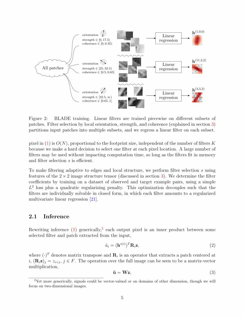
As described e.g. by Weickert [30], the 2× 2 matrix at each pixel location of the smoothedstructure tensor Jρ(∇u) is nonnegative definite with orthogonal eigenvectors. This eigensys-tem is a powerful characterization of the local image geometry. The dominant eigenvectoris a robust spatially-smoothed estimate of the gradient orientation (the direction up to asign ambiguity) while the second eigenvector gives the local edge orientation. The largereigenvalue is a smoothed estimate of the squared gradient magnitude. In other words, theeigensystem of Jρ(∇u) is a spatially-weighted principle components analysis of the raw imagegradient ∇u.

The eigenvalues λ1 ≥ λ2 and dominant eigenvector w of a matrix(a bb c

)can be computed as

λ1,2 = 12

((a+ c)± δ

), (15)

w =

(2b

c− a+ δ

), (16)

where3 δ =√

(a− c)2 + (2b)2. The second eigenvector is the orthogonal complement of w.From the eigensystem, we define the features:

• orientation = arctanw2/w1, is the predominant local orientation of the gradient;

• strength =√λ1, is the local gradient magnitude; and

• coherence =√λ1−√λ2√

λ1+√λ2

, which characterizes the amount of anisotropy in the local struc-

ture.4

3If the matrix is proportional to identity (a = c, b = 0), any vector is an eigenvector of the same eigenvalue.In this edge case, (16) computes w =

(00

), which might be preferable as an isotropic characterization.

4Different works vary in the details of how “coherence” is defined. This is the definition that we use.

9

0 1 23

45

6

7

8

9

10

1112

131415

Orientation

10 40

Strength

0.2 0.8

Coherence

Figure 3: Typical structure tensor feature quantization for BLADE filter selection, using 16orientations, 5 strength bins, and 3 coherence bins.

Orientation

Str

ength

Str

ength

Str

ength

Coh

eren

ce

0

−0.4

0.4

−0.8

0.8

Figure 4: Trained 7 × 7 BLADE filters approximating the bilateral filter with 24 differentorientations, 3 strength values, and 3 coherence values.

3.2 Quantization

We use the three described structure tensor features for filter selection s, bounding anduniformly quantizing each feature to a small number of equal-sized bins, and consideringthem together as a three-dimensional index into the bank of filters.

A typical quantization is shown in Figure 3. The orientation feature is quantized to 16orientations. To avoid asymmetric behavior, orientation quantization is done such thathorizontal and vertical orientations correspond to bin centers. Strength is bounded to [10, 40]and quantized to 5 bins, and coherence is bounded to [0.2, 0.8] and quantized to 3 bins.

4 Learning for Computational Photography

This and the next few sections show the flexibility of our approach by applying BLADE toseveral applications. We begin by demonstrating how BLADE can be used to make fastapproximations to other image processing methods. BLADE can produce a similar effectthat in some cases has lower computational cost than the original method.

10

Input Reference BLADE

Figure 5: Approximation of the bilateral filter. Top row: BLADE has PSNR 35.90 dB andMSSIM 0.9272. Bottom row: BLADE has PSNR 33.41 dB and MSSIM 0.8735.

Filters

0

−0.5

0.5

−1.0

1.0

Filter standard deviation estimates

10−3

10−2

10−1

Figure 6: Example of interpreting failed training. Left: filters. Right: filter standarddeviation estimates. Compare with Figure 4.

4.1 Bilateral filter

The bilateral filter [28] is an edge-adaptive smoothing filter where each output pixel is com-puted from the input as

ui =

∑j Gσr(|zi − zj|)Gσs(‖i− j‖)zj∑j Gσr(|zi − zj|)Gσs(‖i− j‖)

, (17)

11

Orientation

Str

ength

Str

ength

Str

ength

Str

ength

Coh

eren

ce

0

−0.1

0.1

−0.2

0.2

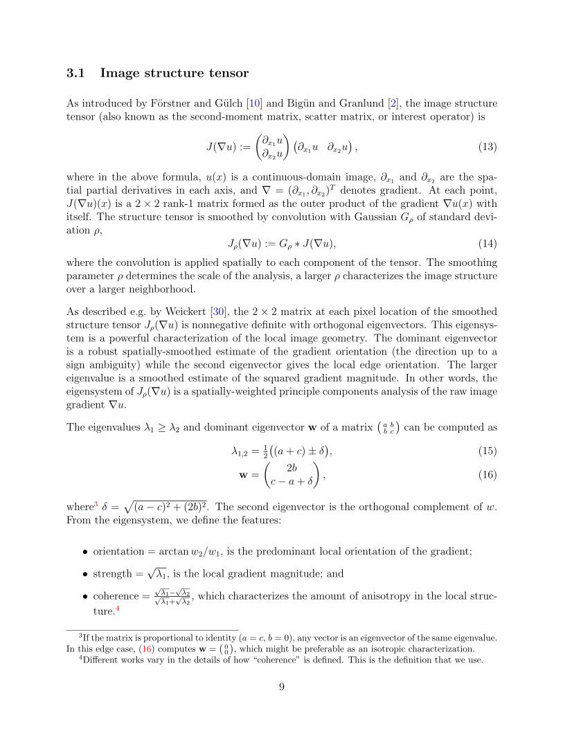
Figure 7: 7 × 7 BLADE filters approximating TV flow with 16 different orientations, 4strength values, and 4 coherence values.

where Gσ denotes a Gaussian kernel with standard deviation σ.

We approximate the bilateral filter where the range kernel has standard deviation σr = 25(relative to a [0, 255] nominal intensity range) and the spatial kernel has standard deviationσs = 2.5 pixels. We use 7 × 7 filters, smoothing strength ρ = 1.2, 24 orientation buckets, 3strength buckets over [10, 35], and 3 coherence buckets over [0.2, 0.8] (Fig. 4).

Over the Kodak Image Suite, bilateral BLADE agrees with the reference bilateral imple-mentation with an average PSNR of 37.30 dB and average MSSIM of 0.9630 and processingeach 768× 512 image costs 18.6 ms on a Xeon E5-1650v3 desktop PC. For comparison, thedomain transform by Gastal and Oliveira [11], specifically developed for efficiently approxi-mating the bilateral filter, agrees with the reference bilateral implementation with an averagePSNR of 42.90 dB and average MSSIM of 0.9855 and costs 5.6 ms. Fig. 5 shows BLADEapproximation of the bilateral filter on a crop from image 17 and 22 of the Kodak ImageSuite.

Number of filters With using fewer filters, the BLADE approximation can be made totrade memory cost for accuracy, which may be attractive on resource constrained platforms.For example, training BLADE using instead 8 orientations, 3 strength buckets, and nobucketing over coherence (24 filters vs. 216 filters above), the approximation accuracy isonly moderately reduced to an average PSNR of 37.00 dB and MSSIM 0.9609. A reasonableapproximation can be made with a small number of filters.

12

Input Reference BLADE

Figure 8: Example of approximated TV flow. Top row: BLADE has PSNR 32.10 dB andMSSIM 0.9369. Bottom row: BLADE has PSNR 35.99 dB and MSSIM 0.9691.

Interpretability To demonstrate the interpretability of BLADE, Figure 6 shows a failedtraining example where we attempted to train BLADE filters for bilateral filtering withstrength range over [10, 80]. Some of the high strength, high coherence buckets receivedfew training patches. Training parameters are otherwise the same as before. The filters areoverly-smooth in the problematic buckets. Additionally, the corresponding filter standarddeviation estimates are large, indicating a training problem.

4.2 TV flow

In this section, we use BLADE to approximate the evolution of an anisotropic diffusionequation, a modification of total variation (TV) flow suggested by Marquina and Osher [16],

∂tu = |∇u| div(∇u/|∇u|) (18)

where u(x) is a continuous-domain image, ∇ denotes spatial gradient, div denotes divergence,and ∂tu is the rate of change of the evolution.

We train 7×7 filters (K = 16×4×4) on a dataset of 32 photograph images of size 1600×1200.We use the second-order finite difference scheme described by Marquina and Osher [16] asthe reference implementation to generate target images for training (Fig. 7).

13

Orientation

Coh

eren

ce

0

−0.2

0.2

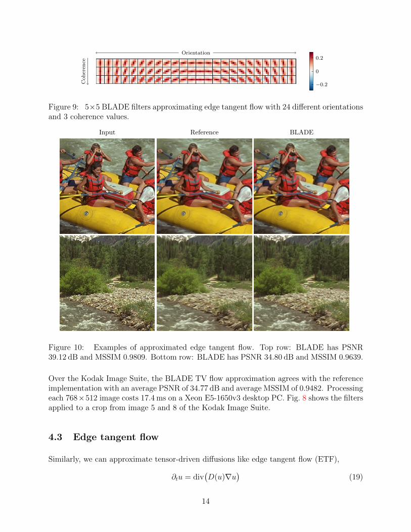
Figure 9: 5×5 BLADE filters approximating edge tangent flow with 24 different orientationsand 3 coherence values.

Input Reference BLADE

Figure 10: Examples of approximated edge tangent flow. Top row: BLADE has PSNR39.12 dB and MSSIM 0.9809. Bottom row: BLADE has PSNR 34.80 dB and MSSIM 0.9639.

Over the Kodak Image Suite, the BLADE TV flow approximation agrees with the referenceimplementation with an average PSNR of 34.77 dB and average MSSIM of 0.9482. Processingeach 768×512 image costs 17.4 ms on a Xeon E5-1650v3 desktop PC. Fig. 8 shows the filtersapplied to a crop from image 5 and 8 of the Kodak Image Suite.

4.3 Edge tangent flow

Similarly, we can approximate tensor-driven diffusions like edge tangent flow (ETF),

∂tu = div(D(u)∇u

)(19)

14

Blend = 0% Blend = 25% Blend = 50% Blend = 75% Blend = 100%

Figure 11: Control filter strength. Blending the identity filter with the edge tangent flowfilter.

where at each point, D(u)(x) is the 2 × 2 outer product of the unit-magnitude local edgetangent orientation. Supposing the edge tangent orientation is everywhere equal to θ, thediffusion (19) reduces to the one-dimensional heat equation along θ, whose solution is con-volution with an oriented Gaussian,

u(t, x) =

∫ ∞−∞

exp(− s2

4t)

√4πt

u(0, x+ θs) ds. (20)

We expect for this reason that the structure tensor orientation matters primarily to approx-imate this diffusion. However, if orientation is not locally constant, the solution is morecomplicated. Therefore, we use also the coherence, which indicates the extent to which theconstant orientation assumption is true (whereas strength gives no such indication, so weexclude it).

We train 5 × 5 filters (K = 24 × 3) over the same dataset, using line integral convolutionevolved with second-order Runge–Kutta as a reference implementation to generate targetimages for training.

Over the Kodak Image Suite, the BLADE ETF approximation agrees with the referenceimplementation with an average PSNR of 40.94 dB and average MSSIM of 0.9849. Processingeach 768 × 512 image costs 14.5 ms on a Xeon E5-1650v3 desktop PC. Figure 10 shows anexample application to a crop from image 13 and 14 of the Kodak Image Suite.

4.4 Control the filter strength

One limitation of using these filters for image processing is that each set of filters is trainedfor a specific set of filter parameters (e.g. our bilateral filter is trained for σr = 25, σs = 2.5),

15

Orientation

Str

ength

Str

ength

Str

ength

Coh

eren

ce

0

−0.3

0.3

−0.6

0.6

Figure 12: 7 × 7 BLADE filters for AWGN denoising with noise standard deviation 20,using ρ = 1.7, 16 different orientations, 5 strength values, and 3 coherence values.

Clean Noisy BLADE denoised

Figure 13: Simple AWGN denoiser example with noise standard deviation 20. The noisyimage has PSNR 22.34 dB and MSSIM 0.5792 and the BLADE denoised image has PSNR28.04 dB and MSSIM 0.8268.

however, it would be interesting to be able to control the strength of the effect withouthaving multiple versions of the filters for different filter parameters. To address this issue,given that each filter knows how to apply the effect for that specific bucket, we interpolateeach filter linearly with the identity filter (i.e., a delta in the origin of the filter). Figure 11shows an example of how we can use this to control the strength of the BLADE ETF filter.

Since we interpolate the filters (which are small compared to the image), the performancepenalty is negligible.

16

Level 0Orig. Resolution

Level 1½ Resolution

Level 2¼ Resolution

Level 3⅛ Resolution

2× bicubic downscale

2× bicubic downscale

2× bicubic downscale

Noisy Input Intermediate Result

Upscaling+Filtering+Blending

Final Result

High ResHigh Noise

Low ResLow Noise

High Res Pixels Low Res PixelsAugmented Feature Vector

LearnUpscaling + Filtering + Blending

Target Pixel

Figure 14: Multilevel BLADE denoising pipeline.

5 Denoising

5.1 A Simple AWGN Denoiser

We build a grayscale image denoiser with an additive white Gaussian noise (AWGN) modelby training a BLADE filter, using a set of clean images as the targets and syntheticallyadding noise to create the observations.

Filters are selected based on the observed image structure tensor analysis (as described insection 3). Since the observed image is noisy, the structure tensor smoothing by Gρ has thecritical role of ameliorating noise before computing structure tensor features. Parameter ρmust be large enough for the noise level to obtain robust filter selection. Figure 12 showsthe trained filters for a noise standard deviation of 20, for which we set ρ = 1.7.

We test the denoiser over the Kodak Image Suite with ten AWGN noise realizations perimage. The noisy input images have average PSNR of 22.31 dB and average MSSIM of0.4030. The simple BLADE denoiser improves the average PSNR to 29.44 dB and MSSIMto 0.7732. Processing each 768× 512 image costs 19.8 ms on a Xeon E5-1650v3 desktop PC.Figure 13 shows an example of denoising a crop of image 5 from the Kodak Image Suite.

5.2 Multiscale AWGN Denoising

We now demonstrate how multiscale application of the previous section enables BLADEto perform fast edge-adaptive image denoising with quality in the ballpark of much moreexpensive methods. We begin by taking an input image and forming an image pyramid by

17

Input Bilateral

BM3D Multiscale BLADE

Figure 15: Qualitative comparison of denoising results.

downsampling by factor of two. Using a bicubic downsampler, which effectively reduce thenoise level by half per level, and is extremely fast. An image pyramid of a target image isalso constructed by using the same downsampling method.

Considering level L as the coarsest level of the image pyramid, we start training from thelevel L− 1 and go up to the finest level. We train filters that operate on a pair of patches,one from the input image at the current level and another at the corresponding position inthe filtered result at the next coarser level, see Figure 14.

We build up denoised results as shown in Figure 14. The filters are learned to optimallyupscale coarser level images and blend them into filtered current level images to create resultsfor next level. Structure tensor analysis is performed on the patches of the current level.

Figure 15 shows a comparison of denoising results among other methods. Multiscale denois-ing results have quality comparable to the state-of-the-art algorithms but with fast processingtime.

18

Orientation

Str

ength

Str

ength

Str

ength

Coh

eren

ce

0

−0.3

0.3

−0.6

0.6

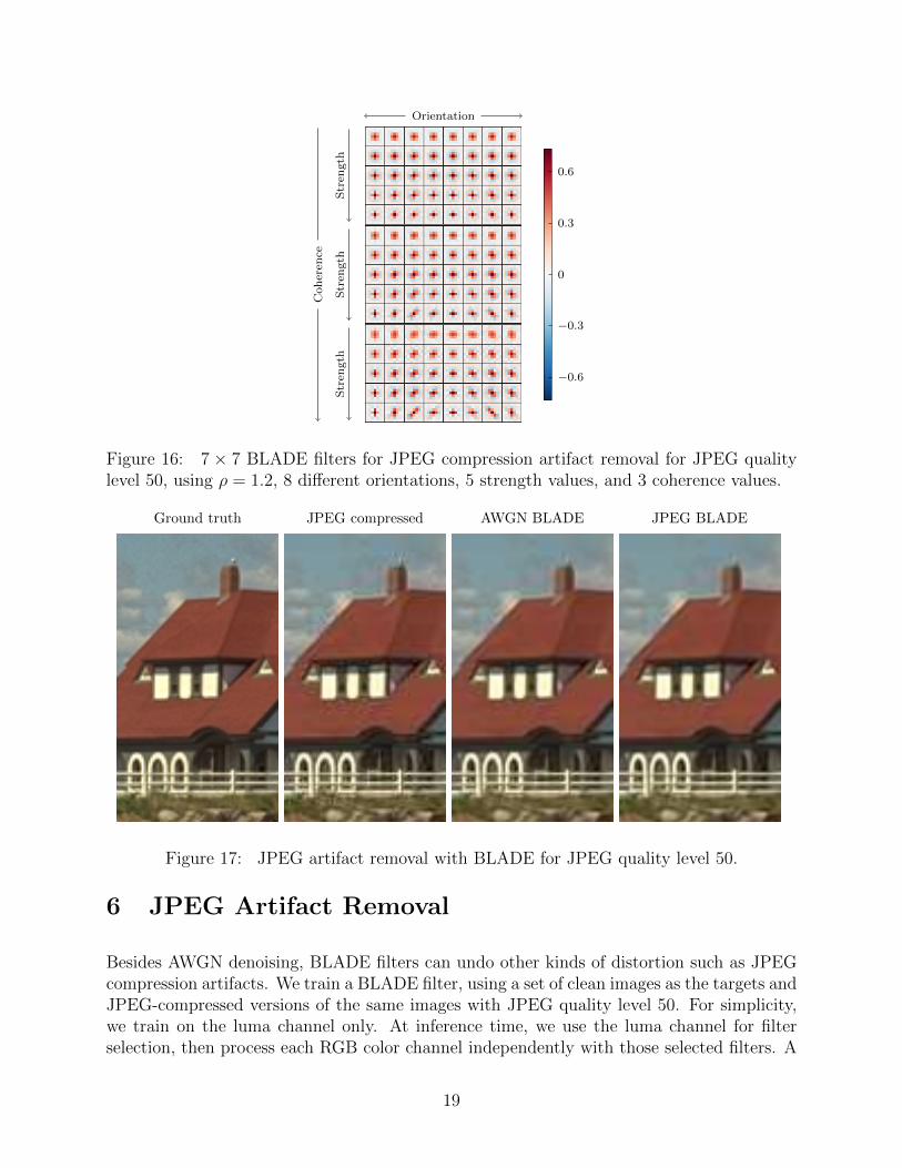
Figure 16: 7 × 7 BLADE filters for JPEG compression artifact removal for JPEG qualitylevel 50, using ρ = 1.2, 8 different orientations, 5 strength values, and 3 coherence values.

Ground truth JPEG compressed AWGN BLADE JPEG BLADE

Figure 17: JPEG artifact removal with BLADE for JPEG quality level 50.

6 JPEG Artifact Removal

Besides AWGN denoising, BLADE filters can undo other kinds of distortion such as JPEGcompression artifacts. We train a BLADE filter, using a set of clean images as the targets andJPEG-compressed versions of the same images with JPEG quality level 50. For simplicity,we train on the luma channel only. At inference time, we use the luma channel for filterselection, then process each RGB color channel independently with those selected filters. A

19

more complicated scheme could train other sets of filters for the Cb and Cr channels.

Fig. 17 shows the filters applied to a crop from image 21 of the Kodak Image Suite. Filteringgreatly reduces the visibility of the 8× 8 block edges and DCT ripples.

JPEG artifact removal is essentially a denoising problem, viewing distortion introducedby the lossy compression as noise. We measure over the Kodak Image Suite that JPEGcompression with quality 50 corresponds to an average MSE of 43.6. For comparison, weshow the results of the simple AWGN BLADE denoiser from section 5.1 trained for AWGNnoise of variance 43.6 (“AWGN BLADE” in Fig. 17). While the AWGN denoiser reducesmuch of the artifacts, the BLADE trained on JPEG is more effective.

Over the Kodak Image Suite, quality level 50 JPEG compression has average PSNR 32.17 dB.AWGN BLADE improves the average PSNR to 32.66 dB, while JPEG BLADE improvesaverage PSNR to 32.75 dB. Indeed, JPEG noise is not AWGN. This shows BLADE takesadvantage of spatial correlations in the noise for which it is trained.

Alternatively, we can account for JPEG’s 8 × 8 block structure by training different filtersper pixel coordinate modulo 8. At the memory cost of 64 times more filters compared to thesingle shift approach above, this extension makes a modest improvement.

7 Demosaicing

In this section, we consider the task of demosaicing using BLADE. In the original RAISRformulation, filters are designed only for single-channel images, and operate on the lumachannel for color images. Demosaicing requires exploiting correlation between color channels,which we do by computing each output sample as a linear combination of samples from allthree channels in the input patch.

For each pixel i, instead of a single-channel filter hs(i) that takes in a single-channel patchand outputs a pixel, we use three filters hs(i),r, hs(i),g, and hs(i),b that compute output red,green, and blue pixels respectively from a given RGB input patch. The resulting inferencebecomes:

uri = (hs(i),r)TRiz

ugi = (hs(i),g)TRiz

ubi = (hs(i),b)TRiz

(21)

where Ri extracts a color patch centered at i, and uri , ugi , and ubi denote the output red,

green, and blue pixels. We interpret this extension as three separate BLADE filterbanksdescribed in Section 2, one for each output color channel.

With this color extension, we then train filters to exploit correlations between color channelsfor demosaicing. Similar to RAISR upscaling, we first apply a fast cheap demosaicing onthe input image, then perform structure tensor analysis and filter selection as usual. For ourexperiments we use the method described in Menon et al. [17].

20

Coh

eren

ce

Filters to Estimate Red Channel

Filters to Estimate Green Channel

Filters to Estimate Blue Channel

Stre

ngth

Stre

ngth

Stre

ngth

Coh

eren

ce Stre

ngth

Stre

ngth

Stre

ngth

Coh

eren

ce Stre

ngth

Stre

ngth

Stre

ngth

Orientation

Orientation

Orientation

Figure 18: Color BLADE filters trained on Menon demosaiced images, with ρ = 0.7, 8difference orientations, 3 strength values, and 3 coherence values. Here, the color map usesthe red, green, and blue components of the filters.

Figure 18 shows the color filters trained on Bayer demosaiced images using the method fromMenon et al. [17] on the Kodak Image Suite, with ρ = 0.7, 8 different orientations, 3 strengthvalues, and 3 coherence values. Three sets of color filters were trained to predict red, green,and blue pixels respectively. As expected, the filters to estimate each color channel mostlyutilize information from the same color channel. For example, the color filters to estimatered channel are mostly red. On the other hand, cross-channel correlation is leveraged as thefilters are not purely red, green, or blue.

We evaluate the demosaicing methods on the Kodak Image Suite. The average PSNR forMenon demosaiced images is 39.14 dB, whereas the average PSNR for our proposed methodis 39.69 dB. Figure 19 shows a cropped example with reduction of demosaicing artifactsusing our proposed method.

21

Ground Truth Menon Proposed

Figure 19: Comparison between Menon and BLADE. Demosaicing with BLADE displaysless artifacts.

CP

Uti

me

(s)

Image size (MP)

1 4 16 640

2

4

13× 13

11× 11

9× 9

7× 7

5× 5

Figure 20: CPU time on Xeon E5-1650v3 desktop PC vs. image size in megapixels.

8 Computational Performance

BLADE filtering has been optimized to run fast on desktop and mobile platforms. Theoptimizations to achieve the desired performance are the following:

• For CPU implementation, the code is optimized using the programming languageHalide [19]. Halide code decouples the algorithm implementation from the schedul-ing. This allows us to create optimized code that uses native vector instructions andparallelizes over multiple CPU cores.

22

Table 1: CPU performance on different devices.Platform 5× 5 filters 7× 7 filters 9× 9 filters 11× filters 13× 13 filters

Xeon E5-1650v3 PC 97.50 MP/s 71.70 MP/s 52.26 MP/s 41.28 MP/s 31.00 MP/sPixel 2017 29.47 MP/s 22.41 MP/s 18.00 MP/s 15.01 MP/s 11.39 MP/sPixel 2016 21.39 MP/s 15.62 MP/s 11.42 MP/s 8.71 MP/s 6.59 MP/sNexus 6P 19.06 MP/s 14.60 MP/s 11.09 MP/s 9.11 MP/s 6.72 MP/s

• BLADE processing on the CPU is performed using low-precision integer arithmeticwhere possible. This allows for a higher degree of vectorization, especially on mobileprocessors, and reduces memory bandwidth. Analogously, the GPU implementationuses 16-bit float arithmetic where possible.

• The algorithm is GPU amenable, we have seen up to an order of magnitude performanceimprovement on GPU over our CPU implementation. The BLADE filter selection mapsefficiently to texture fetches with all filter coefficients stored in a single RGBA texture.It is also possible to process 4 pixels in parallel per pixel shader invocation by takingadvantage of all 4 RGBA channels for processing.

• Approximations to transcendental functions are used where applicable. For examplethe arctangent for orientation angle computation uses a variation of a well-knownquadratic approximation [20].

Our algorithm has runtime linear in the number of output pixels. Figure 20 shows that givena fixed filter size, the performance is linear.

Table 1 shows the performance of BLADE for different platforms on the CPU and differentfilter sizes. A full HD image (1920 × 1080 pixels) takes less than 60 ms to process on themobile devices we tested.

The GPU implementation focuses on the 5× 5 filters, the peak performance are as follows:131.53 MP/s on a Nexus 6P, 150.09 MP/s on a Pixel 2016, 223.03 MP/s on a Pixel 2017.Another way to look at it is that the algorithm is capable of 4k video output (3840 × 2160pixels) at 27 fps or at full HD output at over 100 fps on device.

9 Conclusions

We have presented Best Linear Adaptive Enhancement (BLADE), a framework for simple,trainable, edge-adaptive filtering based on a local linear estimator. BLADE has computa-tionally efficient inference, is easy to train and interpret, and is applicable to a fairly widerange of tasks. Filter selection is not trained; it is performed by hand-crafted features derivedfrom the image structure tensor, which are effective for adapting behavior to the local imagegeometry, but is probably the biggest weakness of our approach from a machine learningperspective and an interesting aspect for future work.

23

x1 x1 + 1

x2

x2 + 1

+1

−1

≈ ∂x′1

x1 x1 + 1

x2

x2 + 1+1

−1

≈ ∂x′2

Figure 21: Diagonal finite differences for approximating the image gradient.

A Numerical details

Implementation of (13) requires a numerical approximation of the image gradient. Forward(or backward) differences could be used, but they are only first-order accurate,

1h

(u(x1 + 1, x2)− u(x1, x2)

)= ∂x1u(x1, x2) + 1

2∂2x21u(x1, x2)h+O(h2), (22)

where h is the width of a pixel. Centered differences are second-order accurate, but theyincrease the footprint of the approximation

12h

(u(x1 + 1, x2)− u(x1 − 1, x2)

)= ∂x1u(x1, x2) + 1

12∂3x31u(x1, x2)h2 +O(h4) (23)

We instead approximate derivatives of 45-rotated axes x′ = 1√2

(1 −11 1

)x with diagonal dif-

ferences as depicted in Figure 21. If interpreted as logically located at cell centers, diagonaldifferences are second-order accurate,

1√2h

(u(x1 + 1, x2)− u(x1, x2 + 1)

)= ∂x′1u(x1 + 1

2, x2 + 1

2) +O(h2), (24)

1√2h

(u(x1 + 1, x2 + 1)− u(x1, x2)

)= ∂x′2u(x1 + 1

2, x2 + 1

2) +O(h2). (25)

We then carry out structure tensor analysis on this 45-rotated and 1/2-sample shiftedgradient approximation. When smoothing with Gρ, a symmetric even-length FIR filter isused in each dimension to compensate for the +1/2 shift. The eigenvector w is rotated backby 45 to compensate for the rotation, w =

(1 1−1 1

)w.

References

[1] Yoshua Bengio. Learning deep architectures for AI. Foundations and Trends in MachineLearning, 2(1):1–127, 2009.

[2] Josef Bigun and Gosta H. Granlund. Optimal orientation detection of linear symmetry.In IEEE First International Conference on Computer Vision, pages 433–438, London,Great Britain, 1987.

[3] Antoni Buades, Bartomeu Coll, and J-M Morel. A non-local algorithm for image de-noising. In IEEE Computer Society Conference on Computer Vision and Pattern Recog-nition, 2005, volume 2, pages 60–65. IEEE, 2005.

24

[4] Priyam Chatterjee and Peyman Milanfar. Clustering-based denoising with locallylearned dictionaries. IEEE Transactions on Image Processing, 18(7):1438–1451, 2009.

[5] Yunjin Chen and Thomas Pock. Trainable nonlinear reaction diffusion: A flexible frame-work for fast and effective image restoration. IEEE Transactions on Pattern Analysisand Machine Intelligence, 39(6):1256–1272, 2017.

[6] Jae-Seok Choi and Munchurl Kim. Single image super-resolution using global regressionbased on multiple local linear mappings. IEEE Transactions on Image Processing,26(3):1300–1314, 2017.

[7] K. Dabov, A. Foi, V. Katkovnik, and K. Egiazarian. Image denoising by sparse 3-D transform-domain collaborative filtering. IEEE Transactions on Image Processing,16(8):2080–2095, 2007.

[8] Kostadin Dabov, Alessandro Foi, Vladimir Katkovnik, and Karen O Egiazarian. Imagerestoration by sparse 3D transform-domain collaborative filtering. In Image Processing:Algorithms and Systems, page 681207, 2008.

[9] Joan Duran and Antoni Buades. Self-similarity and spectral correlation adaptive algo-rithm for color demosaicking. IEEE transactions on image processing, 23(9):4031–4040,2014.

[10] Wolfgang Forstner and Eberhard Gulch. A fast operator for detection and preciselocation of distinct points, corners and centres of circular features. In Proceedings of theIntercomission Conference on Fast Processing of Photogrammetric Data, pages 281–305,1987.

[11] Eduardo SL Gastal and Manuel M Oliveira. Domain transform for edge-aware imageand video processing. In ACM Transactions on Graphics (ToG), volume 30, page 69.ACM, 2011.

[12] Saul B. Gelfand and C.S. Ravishankar. A tree-structured piecewise linear adaptive filter.IEEE Transactions on Information Theory, 39(6):1907–1922, 1993.

[13] Haomiao Jiang, Qiyuan Tian, Joyce Farrell, and Brian Wandell. Learning the imageprocessing pipeline. IEEE Transactions on Image Processing, 2017.

[14] Yifei Lou, Xiaoqun Zhang, Stanley Osher, and Andrea Bertozzi. Image recovery vianonlocal operators. Journal of Scientific Computing, 42(2):185–197, 2010.

[15] Stephane Mallat. Understanding deep convolutional networks. Philosophical Transac-tions of the Royal Society A, 374(2065):20150203, 2016.

[16] Antonio Marquina and Stanley Osher. Explicit algorithms for a new time dependentmodel based on level set motion for nonlinear deblurring and noise removal. SIAMJournal on Scientific Computing, 22(2):387–405, 2000.

25

[17] Daniele Menon, Stefano Andriani, and Giancarlo Calvagno. Demosaicing with direc-tional filtering and a posteriori decision. IEEE Transactions on Image Processing,16(1):132–141, 2007.

[18] Gregoire Montavon, Mikio L. Braun, and Klaus-Robert Muller. Kernel analysis of deepnetworks. Journal of Machine Learning Research, 12(Sep):2563–2581, 2011.

[19] Jonathan Ragan-Kelley, Andrew Adams, Sylvain Paris, Marc Levoy, Saman Amaras-inghe, and Fredo Durand. Decoupling algorithms from schedules for easy optimizationof image processing pipelines. ACM Trans. Graph., 31(4):32:1–32:12, July 2012.

[20] S. Rajan, S. Wang, R. Inkol, and A. Joyal. Efficient approximations for the arctangentfunction. IEEE Signal Processing Magazine, pages 108–111, May 2006.

[21] Yaniv Romano, John Isidoro, and Peyman Milanfar. RAISR: Rapid and Accurate ImageSuper Resolution. IEEE Transactions on Computational Imaging, 3(1):110–125, 2017.

[22] Stefan Roth and Michael J Black. Fields of experts. International Journal of ComputerVision, 82(2):205–229, 2009.

[23] Sean Ryan Fanello, Cem Keskin, Pushmeet Kohli, Shahram Izadi, Jamie Shotton, Anto-nio Criminisi, Ugo Pattacini, and Tim Paek. Filter forests for learning data-dependentconvolutional kernels. In Proceedings of the IEEE Conference on Computer Vision andPattern Recognition, pages 1709–1716, 2014.

[24] Hanno Scharr, Michael J. Black, and Horst W. Haussecker. Image statistics andanisotropic diffusion. In International Conference on Computer Vision 2003, 2003.

[25] Uwe Schmidt and Stefan Roth. Shrinkage fields for effective image restoration. InProceedings of the IEEE Conference on Computer Vision and Pattern Recognition, pages2774–2781, 2014.

[26] Samuel Schulter, Christian Leistner, and Horst Bischof. Fast and accurate image upscal-ing with super-resolution forests. In Proceedings of the IEEE Conference on ComputerVision and Pattern Recognition, pages 3791–3799, 2015.

[27] Ioannis M. Stephanakis, George Stamou, and Stefanos Kollias. Piecewise Wiener filtermodel based on fuzzy partition of local wavelet features for image restoration. In Inter-national Joint Conference on Neural Networks 1999, volume 4, pages 2690–2693. IEEE,1999.

[28] Carlo Tomasi and Roberto Manduchi. Bilateral filtering for gray and color images. InSixth International Conference on Computer Vision, 1998, pages 839–846. IEEE, 1998.

[29] Shengjie Wang, Abdel-rahman Mohamed, Rich Caruana, Jeff Bilmes, Matthai Plilipose,Matthew Richardson, Krzysztof Geras, Gregor Urban, and Ozlem Aslan. Analysis ofdeep neural networks with extended data Jacobian matrix. In International Conferenceon Machine Learning, pages 718–726, 2016.

26

[30] Joachim Weickert. Anisotropic diffusion in image processing, volume 1. TeubnerStuttgart, 1998.

[31] Norbert Wiener. Extrapolation, interpolation, and smoothing of stationary time series,volume 7. MIT Press, Cambridge, MA, 1949.

[32] Li Xu, Jimmy Ren, Qiong Yan, Renjie Liao, and Jiaya Jia. Deep edge-aware filters.In Proceedings of the 32nd International Conference on Machine Learning (ICML-15),pages 1669–1678, 2015.

[33] Guoshen Yu, Guillermo Sapiro, and Stephane Mallat. Solving inverse problems withpiecewise linear estimators: From Gaussian mixture models to structured sparsity. IEEETransactions on Image Processing, 21(5):2481–2499, 2012.

[34] Song Chun Zhu and David Mumford. Prior learning and Gibbs reaction-diffusion. IEEETransactions on Pattern Analysis and Machine Intelligence, 19(11):1236–1250, 1997.

27