Bits, Signals, and Packetsweb.mit.edu/6.02/www/s2012/handouts/part1.pdf · 2012-02-01 · Bits,...
98
Bits, Signals, and Packets An Introduction to Digital Communications & Networks M.I.T. 6.02 Lecture Notes Hari Balakrishnan Christopher J. Terman George C. Verghese M.I.T. Department of EECS Last update: December 2011 c 2008-2012 H. Balakrishnan
Transcript of Bits, Signals, and Packetsweb.mit.edu/6.02/www/s2012/handouts/part1.pdf · 2012-02-01 · Bits,...

Bits, Signals, and PacketsAn Introduction to Digital Communications & Networks
M.I.T. 6.02 Lecture Notes
Hari BalakrishnanChristopher J. Terman
George C. Verghese
M.I.T. Department of EECS
Last update: December 2011
c©2008-2012 H. Balakrishnan

2

Contents
List of Figures 7
List of Tables 9
1 Introduction 11.1 Themes . . . . . . . . . . . . . . . . . . . . . . . . . . . . . . . . . . . . . . . . 31.2 Outline and Plan . . . . . . . . . . . . . . . . . . . . . . . . . . . . . . . . . . 5
2 Information, Entropy, and the Motivation for Source Codes 72.1 Information and Entropy . . . . . . . . . . . . . . . . . . . . . . . . . . . . . . 72.2 Source Codes . . . . . . . . . . . . . . . . . . . . . . . . . . . . . . . . . . . . 112.3 How Much Compression Is Possible? . . . . . . . . . . . . . . . . . . . . . . 132.4 Why Compression? . . . . . . . . . . . . . . . . . . . . . . . . . . . . . . . . . 15
3 Compression Algorithms: Huffman and Lempel-Ziv-Welch (LZW) 193.1 Properties of Good Source Codes . . . . . . . . . . . . . . . . . . . . . . . . . 193.2 Huffman Codes . . . . . . . . . . . . . . . . . . . . . . . . . . . . . . . . . . . 213.3 LZW: An Adaptive Variable-length Source Code . . . . . . . . . . . . . . . . 25
4 Why Digital? Communication Abstractions and Digital Signaling 334.1 Sources of Data . . . . . . . . . . . . . . . . . . . . . . . . . . . . . . . . . . . 334.2 Why Digital? . . . . . . . . . . . . . . . . . . . . . . . . . . . . . . . . . . . . . 344.3 Digital Signaling: Mapping Bits to Signals . . . . . . . . . . . . . . . . . . . . 364.4 Clock and Data Recovery . . . . . . . . . . . . . . . . . . . . . . . . . . . . . 384.5 Line Coding with 8b/10b . . . . . . . . . . . . . . . . . . . . . . . . . . . . . 414.6 Communication Abstractions . . . . . . . . . . . . . . . . . . . . . . . . . . . 42
5 Coping with Bit Errors using Error Correction Codes 455.1 Bit Errors . . . . . . . . . . . . . . . . . . . . . . . . . . . . . . . . . . . . . . . 465.2 The Simplest Code: Replication . . . . . . . . . . . . . . . . . . . . . . . . . . 475.3 Embeddings and Hamming Distance . . . . . . . . . . . . . . . . . . . . . . . 485.4 Linear Block Codes and Parity Calculations . . . . . . . . . . . . . . . . . . . 515.5 Protecting Longer Messages with SEC Codes . . . . . . . . . . . . . . . . . . 59
3

4
6 Convolutional Codes: Construction and Encoding 656.1 Convolutional Code Construction . . . . . . . . . . . . . . . . . . . . . . . . 656.2 Parity Equations . . . . . . . . . . . . . . . . . . . . . . . . . . . . . . . . . . . 676.3 Two Views of the Convolutional Encoder . . . . . . . . . . . . . . . . . . . . 686.4 The Decoding Problem . . . . . . . . . . . . . . . . . . . . . . . . . . . . . . . 706.5 The Trellis . . . . . . . . . . . . . . . . . . . . . . . . . . . . . . . . . . . . . . 72
7 Viterbi Decoding of Convolutional Codes 757.1 The Problem . . . . . . . . . . . . . . . . . . . . . . . . . . . . . . . . . . . . . 757.2 The Viterbi Decoder . . . . . . . . . . . . . . . . . . . . . . . . . . . . . . . . . 777.3 Soft Decision Decoding . . . . . . . . . . . . . . . . . . . . . . . . . . . . . . . 797.4 Achieving Higher and Finer-Grained Rates: Puncturing . . . . . . . . . . . . 807.5 Performance Issues . . . . . . . . . . . . . . . . . . . . . . . . . . . . . . . . . 817.6 Summary . . . . . . . . . . . . . . . . . . . . . . . . . . . . . . . . . . . . . . . 83

List of Figures
1-1 Examples of shared media. . . . . . . . . . . . . . . . . . . . . . . . . . . . . . 4
2-1 H(p) as a function of p, maximum when p = 1/2. . . . . . . . . . . . . . . . . 112-2 Possible grades shown with probabilities, fixed- and variable-length encod-
ings . . . . . . . . . . . . . . . . . . . . . . . . . . . . . . . . . . . . . . . . . . 132-3 Possible grades shown with probabilities and information content. . . . . . 14
3-1 Variable-length code from Figure 2-2 shown in the form of a code tree. . . . 213-2 An example of two non-isomorphic Huffman code trees, both optimal. . . . 233-3 Results from encoding more than one grade at a time. . . . . . . . . . . . . . 243-4 Pseudo-code for the LZW adaptive variable-length encoder. Note that some
details, like dealing with a full string table, are omitted for simplicity. . . . . 263-5 Pseudo-code for LZW adaptive variable-length decoder. . . . . . . . . . . . 263-6 LZW encoding of string “abcabcabcabcabcabcabcabcabcabcabcabc” . . . . . 273-7 LZW decoding of the sequence a, b, c,256,258,257,259,262,261,264,260,266,263, c 28
4-1 Errors accumulate in analog systems. . . . . . . . . . . . . . . . . . . . . . . . 354-2 If the two voltages are adequately spaced apart, we can tolerate a certain
amount of noise. . . . . . . . . . . . . . . . . . . . . . . . . . . . . . . . . . . . 364-3 Picking a simple threshold voltage. . . . . . . . . . . . . . . . . . . . . . . . . 374-4 Sampling continuous-time voltage waveforms for transmission. . . . . . . . 384-5 Transmission using a clock (top) and inferring clock edges from bit transi-
tions between 0 and 1 and vice versa at the receiver (bottom). . . . . . . . . 394-6 The two cases of how the adaptation should work. . . . . . . . . . . . . . . . 404-7 The “big picture”. . . . . . . . . . . . . . . . . . . . . . . . . . . . . . . . . . . 434-8 Expanding on the “big picture”: single link view (top) and the network view
(bottom). . . . . . . . . . . . . . . . . . . . . . . . . . . . . . . . . . . . . . . . 44
5-1 Probability of a decoding error with the replication code that replaces eachbit b with n copies of b. The code rate is 1/n. . . . . . . . . . . . . . . . . . . . 48
5

6
5-2 Codewords separated by a Hamming distance of 2 can be used to detectsingle bit errors. The codewords are shaded in each picture. The picture onthe left is a (2,1) repetition code, which maps 1-bit messages to 2-bit code-words. The code on the right is a (3,2) code, which maps 2-bit messages to3-bit codewords. . . . . . . . . . . . . . . . . . . . . . . . . . . . . . . . . . . . 49
5-3 A 2× 4 arrangement for an 8-bit message with row and column parity. . . . 54
5-4 Example received 8-bit messages. Which, if any, have one error? Which, ifany, have two? . . . . . . . . . . . . . . . . . . . . . . . . . . . . . . . . . . . . 54
5-5 A codeword in systematic form for a block code. Any linear code can betransformed into an equivalent systematic code. . . . . . . . . . . . . . . . . 55
5-6 Venn diagrams of Hamming codes showing which data bits are protectedby each parity bit. . . . . . . . . . . . . . . . . . . . . . . . . . . . . . . . . . . 57
5-7 Dividing a long message into multiple SEC-protected blocks of k bits each,adding parity bits to each constituent block. The red vertical rectangles referto bit errors. . . . . . . . . . . . . . . . . . . . . . . . . . . . . . . . . . . . . . 59
5-8 Interleaving can help recover from burst errors: code each block row-wisewith an SEC, but transmit them in interleaved fashion in columnar order.As long as a set of burst errors corrupts some set of kth bits, the receiver canrecover from all the errors in the burst. . . . . . . . . . . . . . . . . . . . . . . 60
6-1 An example of a convolutional code with two parity bits per message bitand a constraint length (shown in the rectangular window) of three. I.e.,r = 2, K = 3. . . . . . . . . . . . . . . . . . . . . . . . . . . . . . . . . . . . . . 66
6-2 Block diagram view of convolutional coding with shift registers. . . . . . . . 69
6-3 State-machine view of convolutional coding. . . . . . . . . . . . . . . . . . . 69
6-4 When the probability of bit error is less than 1/2, maximum-likelihood de-coding boils down to finding the message whose parity bit sequence, whentransmitted, has the smallest Hamming distance to the received sequence.Ties may be broken arbitrarily. Unfortunately, for an N-bit transmit se-quence, there are 2N possibilities, which makes it hugely intractable to sim-ply go through in sequence because of the sheer number. For instance, whenN = 256 bits (a really small packet), the number of possibilities rivals thenumber of atoms in the universe! . . . . . . . . . . . . . . . . . . . . . . . . . 71
6-5 The trellis is a convenient way of viewing the decoding task and under-standing the time evolution of the state machine. . . . . . . . . . . . . . . . . 72
7-1 The trellis is a convenient way of viewing the decoding task and under-standing the time evolution of the state machine. . . . . . . . . . . . . . . . . 76
7-2 The branch metric for hard decision decoding. In this example, the receivergets the parity bits 00. . . . . . . . . . . . . . . . . . . . . . . . . . . . . . . . . 77
7-3 The Viterbi decoder in action. This picture shows four time steps. Thebottom-most picture is the same as the one just before it, but with only thesurvivor paths shown. . . . . . . . . . . . . . . . . . . . . . . . . . . . . . . . 86

SECTION 7
7-4 The Viterbi decoder in action (continued from Figure 7-3. The decoded mes-sage is shown. To produce this message, start from the final state with small-est path metric and work backwards, and then reverse the bits. At each stateduring the forward pass, it is important to remeber the arc that got us to thisstate, so that the backward pass can be done properly. . . . . . . . . . . . . . 87
7-5 Branch metric for soft decision decoding. . . . . . . . . . . . . . . . . . . . . 887-6 The free distance of a convolutional code. . . . . . . . . . . . . . . . . . . . . 887-7 Error correcting performance results for different rate-1/2 codes. . . . . . . 897-8 Error correcting performance results for three different rate-1/2 convolu-
tional codes. The parameters of the three convolutional codes are (111,110)(labeled “K = 3 glist=(7,6)”), (1110,1101) (labeled “K = 4 glist=(14,13)”),and (111,101) (labeled “K = 3 glist=(7,5)”). The top three curves below theuncoded curve are for hard decision decoding; the bottom three curves arefor soft decision decoding. . . . . . . . . . . . . . . . . . . . . . . . . . . . . . 89

8

List of Tables
6-1 Examples of generator polynomials for rate 1/2 convolutional codes withdifferent constraint lengths. . . . . . . . . . . . . . . . . . . . . . . . . . . . . 68
9

MIT 6.02 DRAFT Lecture NotesLast update: September 6, 2011Comments, questions or bug reports?
Please contact hari at mit.edu
CHAPTER 1Introduction
Our mission is to expose you to a variety of different technologies and techniques in elec-trical engineering and computer science. We will do this by studying several salient prop-erties of digital communication systems, learning both important aspects of their design,and also the basics of how to analyze their performance. Digital communication systemsare well-suited for our goals because they incorporate ideas from a large subset of electricalengineering and computer science.
Equally important, the ability to disseminate and exchange information over theworld’s communication networks has revolutionized the way in which people work, play,and live. At the turn of the century when everyone was feeling centennial and reflective,the U.S. National Academy of Engineering produced a list of 20 technologies that made themost impact on society in the 20th century.1 This list included life-changing innovationssuch as electrification, the automobile, and the airplane; joining them were four technolog-ical achievements in the area of commununication—radio and television, the telephone, theInternet, and computers—whose technological underpinnings we will be most concernedwith in this book.
Somewhat surprisingly, the Internet came in only at #13, but the reason given by thecommittee was that it was developed toward the latter part of the century and that theybelieved the most dramatic and significant impacts of the Internet would occur in the 21stcentury. Looking at the first decade of this century, that sentiment sounds right—the ubiq-uitous spread of wireless networks and mobile devices, the advent of social networks, andthe ability to communicate any time and from anywhere are not just changing the face ofcommerce and our ability to keep in touch with friends, but are instrumental in massivesocietal and political changes.
Communication is fundamental to our modern existence. Who among you can imaginelife without the Internet and its applications and without some form of networked mobiledevice? Most people feel the same way—in early 2011, over 5 billion mobile phones wereactive worldwide, over a billion of which had “broadband” network connectivity. To putthis number (5 billion) in perspective, it is larger than the number of people in the world
1“The Vertiginous March of Technology”, obtained from nae.edu. Document at http://bit.ly/owMoO6
1

2 CHAPTER 1. INTRODUCTION
who (in 2011) have electricity, shoes, toothbrushes, or toilets!2
What makes our communication networks work? This course is a start at understand-ing the answers to this question. This question is worth studying not just because of theimpact that communication systems have had on the world, but also because the technicalareas cover so many different fields in EECS. Before we dive in and describe the “roadmap”for the course, we want to share a bit of the philosophy behind the material.
Traditionally, in both education and in research, much of “low-level communication”has been considered an “EE” topic, covering primarily the issues governing how bits of in-formation move across a single communication link. In a similar vein, much of “network-ing” has been considered a “CS” topic, covering primarily the issues of how to build com-munication networks composed of multiple links. In particular, many traditional courseson “digital communication” rarely concern themselves with how networks are built andhow they work, while most courses on “computer networks” treat the intricacies of com-munication over physical links as a black box. As a result, a sizable number of peoplehave a deep understanding of one or the other topic, but few people are expert in everyaspect of the problem. As an abstraction, however, this division is one way of conquer-ing the immense complexity of the topic, but our goal in this course is to both understandthe important details, and also understand how various abstractions allow different partsof the system to be designed and modified without paying close attention (or even reallyunderstanding) what goes on elsewhere in the system.
One drawback of preserving strong boundaries between different components of a com-munication system is that the details of how things work in another component may re-main a mystery, even to practising engineers. In the context of communication systems,this mystery usually manifests itself as things that are “above my layer” or “below mylayer”. And so although we will appreciate the benefits of abstraction boundaries in thiscourse, an important goal for us is to study the most important principles and ideas thatgo into the complete design of a communication system. Our goal is to convey to you boththe breadth of the field as well as its depth.
In short, we cover communication systems all the way from the source, which has someinformation it wishes to transmit, to packets, which messages are broken into for transmis-sion over a network, to bits, each of which is a “0” or a “1”, to signals, which are analogwaveforms sent over physical communication links (such as wires, fiber-optic cables, ra-dio, or acoustic waves). We describe the salient aspects of all the layers, starting from howan application might encode messages to how the network handles packets to how linksmanipulate bits to how bits are converted to signals for transmission. In the process, wewill study networks of different sizes, ranging from the simplest dedicated point-to-pointlink, to shared media with a set of communicating nodes sharing a common physical com-munication medium, to larger multi-hop networks that themselves are connected to othernetworks to form even bigger networks.
2It is in fact distressing that according to a recent survey conducted by TeleNav—and we can’t tell if thisis a joke—40% of iPhone users say they’d rather give up their toothbrushes for a week than their iPhones!http://www.telenav.com/about/pr-summer-travel/report-20110803.html

SECTION 1.1. THEMES 3
� 1.1 Themes
Three fundamental challenges lie at the heart of all digital communication systems andnetworks: reliability, sharing, and scalability. We will spend a considerable amount of timeon the first two issues in this introductory course, but much less time on the third.
� 1.1.1 Reliability
A large number of factors conspire to make communication unreliable, and we will studynumerous techniques to improve reliability. A common theme across these different tech-niques is that they all use redundancy in creative and efficient ways to provide reliability us-ing unreliable individual components, using the property of independent (or perhaps weaklydependent) failures of these unreliable components to achieve reliability.
The primary challenge is to overcome a wide range of faults and disturbances that oneencounters in practice, including Gaussian noise and interference that distort or corrupt sig-nals, leading to possible bit errors that corrupt bits on a link, to packet losses caused byuncorrectable bit errors, queue overflows, or link and software failures in the network. Allthese problems degrade communication quality.
In practice, we are interested not only in reliability, but also in speed. Most techniques toimprove communication reliability involve some form of redundancy, which reduces thespeed of communication. The essence of many communication systems is how reliabilityand speed tradeoff against one another.
Communication speeds have increased rapidly with time. In the early 1980s, peoplewould connect to the Internet over telephone links at speeds of barely a few kilobits persecond, while today 100 Megabits per second over wireless links on laptops and 1-10 Gi-gabits per second with wired links are commonplace.
We will develop good tools to understand why communication is unreliable and howto overcome the problems that arise. The techniques involve error-correcting codes, han-dling distortions caused by “inter-symbol interference” using a linear time-invariant chan-nel model, retransmission protocols to recover from packet losses that occur for various rea-sons, and developing fault-tolerant routing protocols to find alternate paths in networks toovercome link or node failures.
� 1.1.2 Efficient Sharing
“An engineer can do for a dime what any fool can do for a dollar,” according to folklore. Acommunication network in which every pair of nodes is connected with a dedicated linkwould be impossibly expensive to build for even moderately sized networks. Sharing istherefore inevitable in communication networks because the resources used to communi-cate aren’t cheap. We will study how to share a point-to-point link, a shared medium, andan entire multi-hop network among multiple communications.
We will develop methods to share a common communication medium among nodes, aproblem common to wired media such as broadcast Ethernet, wireless technologies suchas wireless local-area networks (e.g., 802.11 or WiFi), cellular data networks (e.g., “3G”),and satellite networks (see Figure 1-1).
We will study modulation and demodulation, which allow us to transmit signals overdifferent carrier frequencies. In the process, we can ensure that multiple conversations

4 CHAPTER 1. INTRODUCTION
Figure 1-1: Examples of shared media.
share a communication medium by operating at different frequencies.We will study medium access control (MAC) protocols, which are rules that determine
how nodes must behave and react in the network—emulate either time sharing or frequencysharing. In time sharing, each node gets some duration of time to transmit data, with noother node being active. In frequency sharing, we divide the communication bandwidth(i.e., frequency range) amongst the nodes in a way that ensures a dedicated frequencysub-range for different communications, and the different communications can then occurconcurrently without interference. Each scheme has its sweet spot and uses.
We will then turn to multi-hop networks. In these networks, multiple concurrent com-munications between disparate nodes occurs by sharing over the same links. That is, onemight have communication between many different entities all happen over the samephysical links. This sharing is orchestrated by special computers called switches, whichimplement certain operations and protocols. Multi-hop networks are generally controlledin distributed fashion, without any centralized control that determines what each nodedoes. The questions we will address include:
1. How do multiple communications between different nodes share the network?
2. How do messages go from one place to another in the network—this task is faciliatedby routing protocols.
3. How can we communicate information reliably across a multi-hop network (as op-posed to over just a single link or shared medium)?
A word on efficiency is in order. The techniques used to share the network and achievereliability ultimately determine the efficiency of the communication network. In general,one can frame the efficiency question in several ways. One approach is to minimize thecapital expenditure (hardware equipment, software, link costs) and operational expenses(people, rental costs) to build and run a network capable of meeting a set of requirements(such as number of connected devices, level of performance and reliability, etc.). Anotherapproach is to maximize the bang for the buck for a given network by maximizing theamount of “useful work” that can be done over the network. One might measure the“useful work” by calculating the aggregate throughput (in “bits per second”, or at higher

SECTION 1.2. OUTLINE AND PLAN 5
speeds, the more convenient “megabits per second”) achieved by the different communi-cations, the variation of that throughput among the set of nodes, and the average delay(often called the latency, measured usually in milliseconds) achieved by the data transfers.Largely speaking, we will be concerned with throughput and latency in this course, andnot spend much time on the broader (but no less important) questions of cost.
Of late, another aspect of efficiency that has become important in many communica-tion systems is energy consumption. This issue is important both in the context of massivesystems such as large data centers and for mobile computing devices such as laptops andmobile phones. Improving the energy efficiency of these systems is an important problem.
� 1.1.3 Scalability
In addition to reliability and efficient sharing, scalability (i.e., designing networks that scaleto large sizes) is an important design consideration for communication networks. We willonly touch on this issue, leaving most of it to later courses (6.033, 6.829).
� 1.2 Outline and Plan
We have divided the course into four parts: the source, and the three important abstrac-tions (signals, bits, and packets). For pedagogic reasons, we will study them in the ordergiven below.
1. The source. Ultimately, all communication is about a source wishing to send someinformation in the form of messages to a receiver (or to multiple receivers). Hence,it makes sense to understand the mathematical basis for information, to understandhow to encode the material to be sent, and for reasons of efficiency, to understand howbest to compress our messages so that we can send as little data as possible but yetallow the receiver to decode our messages correctly. Chapters 2 and 3 describe thekey ideas behind information, entropy (expectation of information), and source coding,which enables data compression. We will study Huffman codes and the Lempel-Ziv-Welch algorithm, two widely used methods.
2. Bits. The main issue we will deal with here is overcoming bit errors using error-correcting codes, specifically linear block codes and convolutional codes. Thesecodes use interesting and somewhat sophisticated algorithms that cleverly apply re-dundancy to reduce or eliminate bit errors. We conclude this module with a dis-cussion of the capacity of the binary symmetric channel, which is a useful and keyabstraction for this part of the course.
3. Signals. The main issues we will deal with are how to modulate bits over signalsand demodulate signals to recover bits, as well as understanding how distortions ofsignals by communication channels can be modeled using a linear time-invariant (LTI)abstraction. Topics include going between time-domain and frequency-domain rep-resentations of signals, the frequency content of signals, and the frequency responseof channels and filters.
4. Packets. The main issues we will deal with are how to share a medium using a MACprotocol, routing in multi-hop networks, and reliable data transport protocols.

6 CHAPTER 1. INTRODUCTION

MIT 6.02 DRAFT Lecture NotesLast update: September 12, 2011Comments, questions or bug reports?
Please contact hari at mit.edu
CHAPTER 2Information, Entropy, and theMotivation for Source Codes
The theory of information developed by Claude Shannon (SM EE ’40, PhD Math ’40) inthe late 1940s is one of the most impactful ideas of the past century, and has changed thetheory and practice of many fields of technology. The development of communicationsystems and networks has benefited greatly from Shannon’s work. In this chapter, wewill first develop the intution behind information and formally define it as a mathematicalquantity and connect it to another property of data sources, entropy.
We will then show how these notions guide us to efficiently compress and decompress adata source before communicating (or storing) it without distorting the quality of informa-tion being received. A key underlying idea here is coding, or more precisely, source coding,which takes each message (or “symbol”) being produced by any source of data and asso-ciate each message (symbol) with a codeword, while achieving several desirable properties.This mapping between input messages (symbols) and codewords is called a code. Our fo-cus will be on lossless compression (source coding) techniques, where the recipient of anyuncorrupted message can recover the original message exactly (we deal with corruptedbits later in later chapters).
� 2.1 Information and Entropy
One of Shannon’s brilliant insights, building on earlier work by Hartley, was to realize thatregardless of the application and the semantics of the messages involved, a general definition ofinformation is possible. When one abstracts away the details of an application, the task ofcommunicating something between two parties, S and R, boils down to S picking one ofseveral (possibly infinite) messages and sending that message to R. Let’s take the simplestexample, when a sender wishes to send one of two messages—for concreteness, let’s saythat the message is to say which way the British are coming:
• “1” if by land.
• “2” if by sea.
7

8 CHAPTER 2. INFORMATION, ENTROPY, AND THE MOTIVATION FOR SOURCE CODES
(Had the sender been from Course VI, it would’ve almost certainly been “0” if by landand “1” if by sea!)
Let’s say we have no prior knowledge of how the British might come, so each of thesechoices (messages) is equally probable. In this case, the amount of information conveyedby the sender specifying the choice is 1 bit. Intuitively, that bit, which can take on oneof two values, can be used to encode the particular choice. If we have to communicate asequence of such independent events, say 1000 such events, we can encode the outcomeusing 1000 bits of information, each of which specifies the outcome of an associated event.
On the other hand, suppose we somehow knew that the British were far more likelyto come by land than by sea (say, because there is a severe storm forecast). Then, if themessage in fact says that the British are coming by sea, much more information is beingconveyed than if the message said that that they were coming by land. To take another ex-ample, far more information is conveyed by my telling you that the temperature in Bostonon a January day is 75◦F, than if I told you that the temperature is 32◦F!
The conclusion you should draw from these examples is that any quantification of “in-formation” about an event should depend on the probability of the event. The greater theprobability of an event, the smaller the information associated with knowing that the eventhas occurred.
� 2.1.1 Information definition
Using such intuition, Hartley proposed the following definition of the information associ-ated with an event whose probability of occurrence is p:
I ≡ log(1/p) = − log(p). (2.1)
This definition satisfies the basic requirement that it is a decreasing function of p. Butso do an infinite number of functions, so what is the intuition behind using the logarithmto define information? And what is the base of the logarithm?
The second question is easy to address: you can use any base, because loga(1/p) =logb(1/p)/ loga b, for any two bases a and b. Following Shannon’s convention, we will usebase 2,1 in which case the unit of information is called a bit.2
The answer to the first question, why the logarithmic function, is that the resulting defi-nition has several elegant resulting properties, and it is the simplest function that providesthese properties. One of these properties is additivity. If you have two independent events(i.e., events that have nothing to do with each other), then the probability that they bothoccur is equal to the product of the probabilities with which they each occur. What wewould like is for the corresponding information to add up. For instance, the event that itrained in Seattle yesterday and the event that the number of students enrolled in 6.02 ex-ceeds 150 are independent, and if I am told something about both events, the amount ofinformation I now have should be the sum of the information in being told individually ofthe occurrence of the two events.
The logarithmic definition provides us with the desired additivity because, given two
1And we won’t mention the base; if you see a log in this chapter, it will be to base 2 unless we mentionotherwise.
2If we were to use base 10, the unit would be Hartleys, and if we were to use the natural log, base e, it wouldbe nats, but no one uses those units in practice.

SECTION 2.1. INFORMATION AND ENTROPY 9
independent events A and B with probabilities pA and pB,
IA + IB = log(1/pA) + log(1/pB) = log1
pA pB= log
1P(A and B)
.
� 2.1.2 Examples
Suppose that we’re faced with N equally probable choices. What is the information re-ceived when I tell you which of the N choices occurred?
Because the probability of each choice is 1/N, the information is log(1/(1/N)) = log Nbits.
Now suppose there are initially N equally probable choices, and I tell you somethingthat narrows the possibilities down to one of M equally probable choices. How muchinformation have I given you about the choice?
We can answer this question by observing that you now know that the probability ofthe choice narrowing done from N equi-probable possibilities to M equi-probable ones isM/N. Hence, the information you have received is log(1/(M/N)) = log(N/M) bits. (Notethat when M = 1, we get the expected answer of log N bits.)
We can therefore write a convenient rule:
Suppose we have received information that narrows down a set of N equi-probable choices to one of M equi-probable choices. Then, we have receivedlog(N/M) bits of information.
Some examples may help crystallize this concept:
One flip of a fair coinBefore the flip, there are two equally probable choices: heads or tails. After the flip,we’ve narrowed it down to one choice. Amount of information = log2(2/1) = 1 bit.
Roll of two diceEach die has six faces, so in the roll of two dice there are 36 possible combinations forthe outcome. Amount of information = log2(36/1) = 5.2 bits.
Learning that a randomly chosen decimal digit is evenThere are ten decimal digits; five of them are even (0, 2, 4, 6, 8). Amount of informa-tion = log2(10/5) = 1 bit.
Learning that a randomly chosen decimal digit ≥ 5Five of the ten decimal digits are greater than or equal to 5. Amount of information= log2(10/5) = 1 bit.
Learning that a randomly chosen decimal digit is a multiple of 3Four of the ten decimal digits are multiples of 3 (0, 3, 6, 9). Amount of information =log2(10/4) = 1.322 bits.
Learning that a randomly chosen decimal digit is even, ≥ 5, and a multiple of 3Only one of the decimal digits, 6, meets all three criteria. Amount of information =

10 CHAPTER 2. INFORMATION, ENTROPY, AND THE MOTIVATION FOR SOURCE CODES
log2(10/1) = 3.322 bits. Note that this information is same as the sum of the previ-ous three examples: information is cumulative if the joint probability of the eventsrevealed to us factors intothe product of the individual probabilities.
In this example, we can calculate the probability that they all occur together, andcompare that answer with the product of the probabilities of each of them occurringindividually. Let event A be “the digit is even”, event B be “the digit is≥ 5, and eventC be “the digit is a multiple of 3”. Then, P(A and B and C) = 1/10 because there isonly one digit, 6, that satisfies all three conditions. P(A) · P(B) · P(C) = 1/2 · 1/2 ·4/10 = 1/10 as well. The reason information adds up is that log(1/P(AandBandC) =log 1/P(A) + log 1/P(B) + log(1/P(C).
Note that pairwise indepedence between events is actually not necessary for informa-tion from three (or more) events to add up. In this example, P(AandB) = P(A) ·P(B|A) = 1/2 · 2/5 = 1/5, while P(A) · P(B) = 1/2 · 1/2 = 1/4.
Learning that a randomly chosen decimal digit is a primeFour of the ten decimal digits are primes—2, 3, 5, and 7. Amount of information =log2(10/4) = 1.322 bits.
Learning that a randomly chosen decimal digit is even and primeOnly one of the decimal digits, 2, meets both criteria. Amount of information =log2(10/1) = 3.322 bits. Note that this quantity is not the same as the sum of theinformation contained in knowing that the digit is even and the digit is prime. Thereason is that those events are not independent: the probability that a digit is evenand prime is 1/10, and is not the product of the probabilities of the two events (i.e.,not equal to 1/2× 4/10).
To summarize: more information is received when learning of the occurrence of anunlikely event (small p) than learning of the occurrence of a more likely event (large p).The information learned from the occurrence of an event of probability p is defined to belog(1/p).
� 2.1.3 Entropy
Now that we know how to measure the information contained in a given event, we canquantify the expected information in a set of possible outcomes. Specifically, if an event ioccurs with probability pi,1 ≤ i ≤ N out of a set of N events, then the average or expectedinformation is given by
H(p1, p2, . . . pN) =N
∑i=1
pi log(1/pi). (2.2)
H is also called the entropy (or Shannon entropy) of the probability distribution. Likeinformation, it is also measured in bits. It is simply the sum of several terms, each of whichis the information of a given event weighted by the probability of that event occurring. Itis often useful to think of the entropy as the average or expected uncertainty associated withthis set of events.
In the important special case of two mutually exclusive events (i.e., exactly one of the two

SECTION 2.2. SOURCE CODES 11
Figure 2-1: H(p) as a function of p, maximum when p = 1/2.
events can occur), occuring with probabilities p and 1− p, respectively, the entropy
H(p,1− p) = −p log p− (1− p) log(1− p). (2.3)
We will be lazy and refer to this special case, H(p,1− p) as simply H(p).This entropy as a function of p is plotted in Figure 2-1. It is symmetric about p = 1/2,
with its maximum value of 1 bit occuring when p = 1/2. Note that H(0) = H(1) = 0;although log(1/p)→∞ as p→ 0, limp→0 p log(1/p)→ 0.
It is easy to verify that the expression for H from Equation (2.2) is always non-negative.Moreover, H(p1, p2, . . . pN) ≤ log N always.
� 2.2 Source Codes
We now turn to the problem of source coding, i.e., taking a set of messages that need to besent from a sender and encoding them in a way that is efficient. The notions of informationand entropy will be fundamentally important in this effort.
Many messages have an obvious encoding, e.g., an ASCII text file consists of sequenceof individual characters, each of which is independently encoded as a separate byte. Thereare other such encodings: images as a raster of color pixels (e.g., 8 bits each of red, greenand blue intensity), sounds as a sequence of samples of the time-domain audio waveform,etc. What makes these encodings so popular is that they are produced and consumedby our computer’s peripherals—characters typed on the keyboard, pixels received from adigital camera or sent to a display, and digitized sound samples output to the computer’saudio chip.
All these encodings involve a sequence of fixed-length symbols, each of which can be

12 CHAPTER 2. INFORMATION, ENTROPY, AND THE MOTIVATION FOR SOURCE CODES
easily manipulated independently. For example, to find the 42nd character in the file, onejust looks at the 42nd byte and interprets those 8 bits as an ASCII character. A text filecontaining 1000 characters takes 8000 bits to store. If the text file were HTML to be sentover the network in response to an HTTP request, it would be natural to send the 1000bytes (8000 bits) exactly as they appear in the file.
But let’s think about how we might compress the file and send fewer than 8000 bits. Ifthe file contained English text, we’d expect that the letter e would occur more frequentlythan, say, the letter x. This observation suggests that if we encoded e for transmissionusing fewer than 8 bits—and, as a trade-off, had to encode less common characters, like x,using more than 8 bits—we’d expect the encoded message to be shorter on average than theoriginal method. So, for example, we might choose the bit sequence 00 to represent e andthe code 100111100 to represent x.
This intuition is consistent with the definition of the amount of information: commonlyoccurring symbols have a higher pi and thus convey less information, so we need fewerbits to encode such symbols. Similarly, infrequently occurring symbols like x have a lowerpi and thus convey more information, so we’ll use more bits when encoding such sym-bols. This intuition helps meet our goal of matching the size of the transmitted data to theinformation content of the message.
The mapping of information we wish to transmit or store into bit sequences is referredto as a code. Two examples of codes (fixed-length and variable-length) are shown in Fig-ure 2-2, mapping different grades to bit sequences in one-to-one fashion. The fixed-lengthcode is straightforward, but the variable-length code is not arbitrary, but has been carefullydesigned, as we will soon learn. Each bit sequence in the code is called a codeword.
When the mapping is performed at the source of the data, generally for the purposeof compressing the data (ideally, to match the expected number of bits to the underlyingentropy), the resulting mapping is called a source code. Source codes are distinct fromchannel codes we will study in later chapters. Source codes remove redundancy and com-press the data, while channel codes add redundancy in a controlled way to improve the errorresilience of the data in the face of bit errors and erasures caused by imperfect communi-cation channels. This chapter and the next are about source codes.
We can generalize this insight about encoding common symbols (such as the letter e)more succinctly than uncommon symbols into a strategy for variable-length codes:
Send commonly occurring symbols using shorter codewords (fewer bits) andinfrequently occurring symbols using longer codewords (more bits).
We’d expect that, on average, encoding the message with a variable-length code wouldtake fewer bits than the original fixed-length encoding. Of course, if the message were allx’s the variable-length encoding would be longer, but our encoding scheme is designed tooptimize the expected case, not the worst case.
Here’s a simple example: suppose we had to design a system to send messages con-taining 1000 6.02 grades of A, B, C and D (MIT students rarely, if ever, get an F in 6.02 ¨̂ ).Examining past messages, we find that each of the four grades occurs with the probabilitiesshown in Figure 2-2.
With four possible choices for each grade, if we use the fixed-length encoding, we need2 bits to encode a grade, for a total transmission length of 2000 bits when sending 1000grades.

SECTION 2.3. HOW MUCH COMPRESSION IS POSSIBLE? 13
Grade Probability Fixed-length Code Variable-length CodeA 1/3 00 10
B 1/2 01 0
C 1/12 10 110
D 1/12 11 111
Figure 2-2: Possible grades shown with probabilities, fixed- and variable-length encodings
Fixed-length encoding for BCBAAB: 01 10 01 00 00 01 (12 bits)
With a fixed-length code, the size of the transmission doesn’t depend on the actualmessage—sending 1000 grades always takes exactly 2000 bits.
Decoding a message sent with the fixed-length code is straightforward: take each pairof received bits and look them up in the table above to determine the corresponding grade.Note that it’s possible to determine, say, the 42nd grade without decoding any other of thegrades—just look at the 42nd pair of bits.
Using the variable-length code, the number of bits needed for transmitting 1000 gradesdepends on the grades.
Variable-length encoding for BCBAAB: 0 110 0 10 10 0 (10 bits)
If the grades were all B, the transmission would take only 1000 bits; if they were all C’s andD’s, the transmission would take 3000 bits. But we can use the grade probabilities givenin Figure 2-2 to compute the expected length of a transmission as
1000[(13
)(2) + (12
)(1) + (1
12)(3) + (
112
)(3)] = 1000[123
] = 1666.7 bits
So, on average, using the variable-length code would shorten the transmission of 1000grades by 333 bits, a savings of about 17%. Note that to determine, say, the 42nd grade, wewould need to decode the first 41 grades to determine where in the encoded message the42nd grade appears.
Using variable-length codes looks like a good approach if we want to send fewer bitson average, but preserve all the information in the original message. On the downside,we give up the ability to access an arbitrary message symbol without first decoding themessage up to that point.
One obvious question to ask about a particular variable-length code: is it the best en-coding possible? Might there be a different variable-length code that could do a better job,i.e., produce even shorter messages on the average? How short can the messages be on theaverage? We turn to this question next.
� 2.3 How Much Compression Is Possible?
Ideally we’d like to design our compression algorithm to produce as few bits as possible:just enough bits to represent the information in the message, but no more. Ideally, wewill be able to use no more bits than the amount of information, as defined in Section 2.1,contained in the message, at least on average.

14 CHAPTER 2. INFORMATION, ENTROPY, AND THE MOTIVATION FOR SOURCE CODES
Specifically, the entropy, defined by Equation (2.2), tells us the expected amount of in-formation in a message, when the message is drawn from a set of possible messages, eachoccurring with some probability. The entropy is a lower bound on the amount of informa-tion that must be sent, on average, when transmitting data about a particular choice.
What happens if we violate this lower bound, i.e., we send fewer bits on the averagethan called for by Equation (2.2)? In this case the receiver will not have sufficient informa-tion and there will be some remaining ambiguity—exactly what ambiguity depends on theencoding, but to construct a code of fewer than the required number of bits, some of thechoices must have been mapped into the same encoding. Thus, when the recipient receivesone of the overloaded encodings, it will not have enough information to unambiguouslydetermine which of the choices actually occurred.
Equation (2.2) answers our question about how much compression is possible by givingus a lower bound on the number of bits that must be sent to resolve all ambiguities at therecipient. Reprising the example from Figure 2-2, we can update the figure using Equation(2.1).
Grade pi log2(1/pi)A 1/3 1.58 bits
B 1/2 1 bit
C 1/12 3.58 bits
D 1/12 3.58 bits
Figure 2-3: Possible grades shown with probabilities and information content.
Using equation (2.2) we can compute the information content when learning of a particulargrade:
N
∑i=1
pi log2(1pi
) = (13
)(1.58) + (12
)(1) + (1
12)(3.58) + (
112
)(3.58) = 1.626 bits
So encoding a sequence of 1000 grades requires transmitting 1626 bits on the average. Thevariable-length code given in Figure 2-2 encodes 1000 grades using 1667 bits on the aver-age, and so doesn’t achieve the maximum possible compression. It turns out the examplecode does as well as possible when encoding one grade at a time. To get closer to the lowerbound, we would need to encode sequences of grades—more on this idea below.
Finding a “good” code—one where the length of the encoded message matches theinformation content (i.e., the entropy)—is challenging and one often has to think “outsidethe box”. For example, consider transmitting the results of 1000 flips of an unfair coinwhere probability of heads is given by pH. The information content in an unfair coin flipcan be computed using equation (2.3):
pH log2(1/pH) + (1− pH) log2(1/(1− pH))
For pH = 0.999, this entropy evaluates to .0114. Can you think of a way to encode 1000unfair coin flips using, on average, just 11.4 bits? The recipient of the encoded messagemust be able to tell for each of the 1000 flips which were heads and which were tails. Hint:

SECTION 2.4. WHY COMPRESSION? 15
with a budget of just 11 bits, one obviously can’t encode each flip separately!In fact, some effective codes leverage the context in which the encoded message is be-
ing sent. For example, if the recipient is expecting to receive a Shakespeare sonnet, thenit’s possible to encode the message using just 8 bits if one knows that there are only 154Shakespeare sonnets. That is, if the sender and receiver both know the sonnets, and thesender just wishes to tell the receiver which sonnet to read or listen to, he can do that usinga very small number of bits, just log 154 bits if all the sonnets are equi-probable!
� 2.4 Why Compression?
There are several reasons for using compression:
• Shorter messages take less time to transmit and so the complete message arrivesmore quickly at the recipient. This is good for both the sender and recipient sinceit frees up their network capacity for other purposes and reduces their networkcharges. For high-volume senders of data (such as Google, say), the impact of send-ing half as many bytes is economically significant.
• Using network resources sparingly is good for all the users who must share theinternal resources (packet queues and links) of the network. Fewer resources permessage means more messages can be accommodated within the network’s resourceconstraints.
• Over error-prone links with non-negligible bit error rates, compressing messages be-fore they are channel-coded using error-correcting codes can help improve through-put because all the redundancy in the message can be designed in to improve errorresilience, after removing any other redundancies in the original message. It is betterto design in redundancy with the explicit goal of correcting bit errors, rather thanrely on whatever sub-optimal redundancies happen to exist in the original message.
Compression is traditionally thought of as an end-to-end function, applied as part of theapplication-layer protocol. For instance, one might use lossless compression between aweb server and browser to reduce the number of bits sent when transferring a collection ofweb pages. As another example, one might use a compressed image format such as JPEGto transmit images, or a format like MPEG to transmit video. However, one may also ap-ply compression at the link layer to reduce the number of transmitted bits and eliminateredundant bits (before possibly applying an error-correcting code over the link). Whenapplied at the link layer, compression only makes sense if the data is inherently compress-ible, which means it cannot already be compressed and must have enough redundancy toextract compression gains.
The next chapter describes two compression (source coding) schemes: Huffman Codesand Lempel-Ziv-Welch (LZW) compression.
� Exercises
1. Several people at a party are trying to guess a 3-bit binary number. Alice is told thatthe number is odd; Bob is told that it is not a multiple of 3 (i.e., not 0, 3, or 6); Charlie

16 CHAPTER 2. INFORMATION, ENTROPY, AND THE MOTIVATION FOR SOURCE CODES
is told that the number contains exactly two 1’s; and Deb is given all three of theseclues. How much information (in bits) did each player get about the number?
2. After careful data collection, Alyssa P. Hacker observes that the probability of“HIGH” or “LOW” traffic on Storrow Drive is given by the following table:
HIGH traffic level LOW traffic levelIf the Red Sox are playing P(HIGH traffic) = 0.999 P(LOW traffic) = 0.001
If the Red Sox are not playing P(HIGH traffic) = 0.25 P(LOW traffic) = 0.75
(a) If it is known that the Red Sox are playing, then how much information in bitsis conveyed by the statement that the traffic level is LOW. Give your answer asa mathematical expression.
(b) Suppose it is known that the Red Sox are not playing. What is the entropyof the corresponding probability distribution of traffic? Give your answer as amathematical expression.
3. X is an unknown 4-bit binary number picked uniformly at random from the set of allpossible 4-bit numbers. You are given another 4-bit binary number, Y, and told thatthe Hamming distance between X (the unknown number) and Y (the number youknow) is two. How many bits of information about X have you been given?
4. In Blackjack the dealer starts by dealing 2 cards each to himself and his opponent:one face down, one face up. After you look at your face-down card, you know a totalof three cards. Assuming this was the first hand played from a new deck, how manybits of information do you have about the dealer’s face down card after having seenthree cards?
5. The following table shows the undergraduate and MEng enrollments for the Schoolof Engineering.
Course (Department) # of students % of totalI (Civil & Env.) 121 7%II (Mech. Eng.) 389 23%III (Mat. Sci.) 127 7%VI (EECS) 645 38%X (Chem. Eng.) 237 13%XVI (Aero & Astro) 198 12%Total 1717 100%
(a) When you learn a randomly chosen engineering student’s department you getsome number of bits of information. For which student department do you getthe least amount of information?
(b) After studying Huffman codes in the next chapter, design a Huffman code toencode the departments of randomly chosen groups of students. Show yourHuffman tree and give the code for each course.

SECTION 2.4. WHY COMPRESSION? 17
(c) If your code is used to send messages containing only the encodings of the de-partments for each student in groups of 100 randomly chosen students, what isthe average length of such messages?
6. You’re playing an online card game that uses a deck of 100 cards containing 3 Aces,7 Kings, 25 Queens, 31 Jacks and 34 Tens. In each round of the game the cards areshuffled, you make a bet about what type of card will be drawn, then a single cardis drawn and the winners are paid off. The drawn card is reinserted into the deckbefore the next round begins.
(a) How much information do you receive when told that a Queen has been drawnduring the current round?
(b) Give a numeric expression for the information content received when learningabout the outcome of a round.
(c) After you learn about Huffman codes in the next chapter, construct a variable-length Huffman encoding that minimizes the length of messages that report theoutcome of a sequence of rounds. The outcome of a single round is encoded asA (ace), K (king), Q (queen), J (jack) or X (ten). Specify your encoding for eachof A, K, Q, J and X.
(d) Again, after studying Huffman codes, use your code from part (c) to calculatethe expected length of a message reporting the outcome of 1000 rounds (i.e., amessage that contains 1000 symbols)?
(e) The Nevada Gaming Commission regularly receives messages in which the out-come for each round is encoded using the symbols A, K, Q, J, and X. They dis-cover that a large number of messages describing the outcome of 1000 rounds(i.e., messages with 1000 symbols) can be compressed by the LZW algorithminto files each containing 43 bytes in total. They decide to issue an indictmentfor running a crooked game. Why did the Commission issue the indictment?
7. Consider messages made up entirely of vowels (A, E, I, O,U). Here’s a table of prob-abilities for each of the vowels:
l pl log2(1/pl) pl log2(1/pl)A 0.22 2.18 0.48E 0.34 1.55 0.53I 0.17 2.57 0.43O 0.19 2.40 0.46U 0.08 3.64 0.29
Totals 1.00 12.34 2.19
(a) Give an expression for the number of bits of information you receive whenlearning that a particular vowel is either I or U.
(b) After studying Huffman codes in the next chapter, use Huffman’s algorithmto construct a variable-length code assuming that each vowel is encoded indi-vidually. Draw a diagram of the Huffman tree and give the encoding for eachof the vowels.

18 CHAPTER 2. INFORMATION, ENTROPY, AND THE MOTIVATION FOR SOURCE CODES
(c) Using your code from part (B) above, give an expression for the expected lengthin bits of an encoded message transmitting 100 vowels.
(d) Ben Bitdiddle spends all night working on a more complicated encoding algo-rithm and sends you email claiming that using his code the expected length inbits of an encoded message transmitting 100 vowels is 197 bits. Would you paygood money for his implementation?

MIT 6.02 DRAFT Lecture NotesLast update: September 12, 2011Comments, questions or bug reports?
Please contact hari at mit.edu
CHAPTER 3Compression Algorithms: Huffman
and Lempel-Ziv-Welch (LZW)
This chapter discusses source coding, specifically two algorithms to compress messages(i.e., a sequence of symbols). The first, Huffman coding, is efficient when one knows theprobabilities of the different symbols one wishes to send. In the context of Huffman cod-ing, a message can be thought of as a sequence of symbols, with each symbol drawn in-dependently from some known distribution. The second, LZW (for Lempel-Ziv-Welch) isan adaptive compression algorithm that does not assume any a priori knowledge of thesymbol probabilities. Both Huffman codes and LZW are widely used in practice, and area part of many real-world standards such as GIF, JPEG, MPEG, MP3, and more.
� 3.1 Properties of Good Source Codes
Suppose the source wishes to send a message, i.e., a sequence of symbols, drawn fromsome alphabet. The alphabet could be text, it could be bit sequences corresponding toa digitized picture or video obtained from a digital or analog source (we will look at anexample of such a source in more detail in the next chapter), or it could be something moreabstract (e.g., “ONE” if by land and “TWO” if by sea, or h for heavy traffic and ` for lighttraffic on a road).
A code is a mapping between symbols and codewords. The reason for doing the map-ping is that we would like to adapt the message into a form that can be manipulated (pro-cessed), stored, and transmitted over communication channels. Codewords made of bits(“zeroes and ones”) are a convenient and effective way to achieve this goal.
For example, if we want to communicate the grades of students in 6.02, we might usethe following encoding:
“A”→ 1“B”→ 01“C”→ 000“D”→ 001
19

20 CHAPTER 3. COMPRESSION ALGORITHMS: HUFFMAN AND LEMPEL-ZIV-WELCH (LZW)
Then, if we want to transmit a sequence of grades, we might end up sending a messagesuch as 0010001110100001. The receiver can decode this received message as the sequenceof grades “DCAAABCB” by looking up the appropriate contiguous and non-overlappingsubstrings of the received message in the code (i.e., the mapping) shared by it and thesource.
Instantaneous codes. A useful property for a code to possess is that a symbol correspond-ing to a received codeword be decodable as soon as the corresponding codeword is re-ceived. Such a code is called an instantaneous code. The example above is an instanta-neous code. The reason is that if the receiver has already decoded a sequence and nowreceives a “1”, then it knows that the symbol must be “A”. If it receives a “0”, then it looksat the next bit; if that bit is “1”, then it knows the symbol is “B”; if the next bit is instead“0”, then it does not yet know what the symbol is, but the next bit determines uniquelywhether the symbol is “C” (if “0”) or “D” (if “1”). Hence, this code is instantaneous.
Code trees and prefix-free codes. A convenient way to visualize codes is using a code tree,as shown in Figure 3-1 for an instantaneous code with the following encoding:
“A”→ 10“B”→ 0“C”→ 110“D”→ 111
In general, a code tree is a binary tree with the symbols at the nodes of the tree and theedges of the tree are labeled with “0” or “1” to signify the encoding. To find the encodingof a symbol, the receiver simply walks the path from the root (the top-most node) to thatsymbol, emitting the label on the edges traversed.
If, in a code tree, the symbols are all at the leaves, then the code is said to be prefix-free,because no codeword is a prefix of another codeword. Prefix-free codes (and code trees)are naturally instantaneous, which makes them attractive.1
Expected code length. Our final definition is for the expected length of a code. Given Nsymbols, with symbol i occurring with probability pi, if we have a code in which symbol ihas length li in the code tree (i.e., the codeword is `i bits long), then the expected length ofthe code is ∑
Ni=1 pi`i.
In general, codes with small expected code length are interesting and useful becausethey allow us to compress messages, delivering messages without any loss of informationbut consuming fewer bits than without the code. Because one of our goals in designingcommunication systems is efficient sharing of the communication links among differentusers or conversations, the ability to send data in as few bits as possible is important.
We say that a code is optimal if its expected code length, L, is the minimum amongall possible codes. The corresponding code tree gives us the optimal mapping betweensymbols and codewords, and is usually not unique. Shannon proved that the expectedcode length of any decodable code cannot be smaller than the entropy, H, of the underlyingprobability distribution over the symbols. He also showed the existence of codes thatachieve entropy asymptotically, as the length of the coded messages approaches∞. Thus,
1Somewhat unfortunately, several papers and books use the term “prefix code” to mean the same thing asa “prefix-free code”. Caveat emptor.

SECTION 3.2. HUFFMAN CODES 21
an optimal code will have an expected code length that “matches” the entropy for longmessages.
The rest of this chapter describes two optimal codes. First, Huffman codes, which areoptimal instantaneous codes when the probabilities of the various symbols are given andwe restrict ourselves to mapping individual symbols to codewords. It is a prefix-free,instantaneous code, satisfying the property H ≤ L ≤ H + 1. Second, the LZW algorithm,which adapts to the actual distribution of symbols in the message, not relying on any apriori knowledge of symbol probabilities.
� 3.2 Huffman Codes
Huffman codes give an efficient encoding for a list of symbols to be transmitted, whenwe know their probabilities of occurrence in the messages to be encoded. We’ll use theintuition developed in the previous chapter: more likely symbols should have shorter en-codings, less likely symbols should have longer encodings.
If we draw the variable-length code of Figure 2-2 as a code tree, we’ll get some insightinto how the encoding algorithm should work:
Figure 3-1: Variable-length code from Figure 2-2 shown in the form of a code tree.
To encode a symbol using the tree, start at the root and traverse the tree until you reachthe symbol to be encoded—the encoding is the concatenation of the branch labels in theorder the branches were visited. The destination node, which is always a “leaf” node foran instantaneous or prefix-free code, determines the path, and hence the encoding. So B isencoded as 0, C is encoded as 110, and so on. Decoding complements the process, in thatnow the path (codeword) determines the symbol, as described in the previous section. So111100 is decoded as: 111→ D, 10→ A, 0→ B.
Looking at the tree, we see that the more probable symbols (e.g., B) are near the root ofthe tree and so have short encodings, while less-probable symbols (e.g., C or D) are furtherdown and so have longer encodings. David Huffman used this observation while writinga term paper for a graduate course taught by Bob Fano here at M.I.T. in 1951 to devise analgorithm for building the decoding tree for an optimal variable-length code.
Huffman’s insight was to build the decoding tree bottom up, starting with the least prob-able symbols and applying a greedy strategy. Here are the steps involved, along with aworked example based on the variable-length code in Figure 2-2. The input to the algo-rithm is a set of symbols and their respective probabilities of occurrence. The output is thecode tree, from which one can read off the codeword corresponding to each symbol.

22 CHAPTER 3. COMPRESSION ALGORITHMS: HUFFMAN AND LEMPEL-ZIV-WELCH (LZW)
1. Input: A set S of tuples, each tuple consisting of a message symbol and its associatedprobability.
Example: S← {(0.333, A), (0.5, B), (0.083, C), (0.083, D)}
2. Remove from S the two tuples with the smallest probabilities, resolving ties arbitrar-ily. Combine the two symbols from the removed tuples to form a new tuple (whichwill represent an interior node of the code tree). Compute the probability of this newtuple by adding the two probabilities from the tuples. Add this new tuple to S. (If Shad N tuples to start, it now has N− 1, because we removed two tuples and addedone.)
Example: S← {(0.333, A), (0.5, B), (0.167, C∧ D)}
3. Repeat step 2 until S contains only a single tuple. (That last tuple represents the rootof the code tree.)
Example, iteration 2: S← {(0.5, B), (0.5, A∧ (C∧ D))}Example, iteration 3: S← {(1.0, B∧ (A∧ (C∧ D)))}
Et voila! The result is a code tree representing a variable-length code for the given symbolsand probabilities. As you’ll see in the Exercises, the trees aren’t always “tall and thin” withthe left branch leading to a leaf; it’s quite common for the trees to be much “bushier.” Asa simple example, consider input symbols A, B, C, D, E, F, G, H with equal probabilitiesof occurrences (1/8 for each). In the first pass, one can pick any two as the two lowest-probability symbols, so let’s pick A and B without loss of generality. The combined ABsymbol has probability 1/4, while the other six symbols have probability 1/8 each. In thenext iteration, we can pick any two of the symbols with probability 1/8, say C and D.Continuing this process, we see that after four iterations, we would have created four setsof combined symbols, each with probability 1/4 each. Applying the algorithm, we findthat the code tree is a complete binary tree where every symbol has a codeword of length3, corresponding to all combinations of 3-bit words (000 through 111).
Huffman codes have the biggest reduction in the expected length of the encoded mes-sage when some symbols are substantially more probable than other symbols. If all sym-bols are equiprobable, then all codewords are roughly the same length, and there are(nearly) fixed-length encodings whose expected code lengths approach entropy and arethus close to optimal.
� 3.2.1 Properties of Huffman Codes
We state some properties of Huffman codes here. We don’t prove these properties formally,but provide intuition about why they hold.
Non-uniqueness. In a trivial way, because the 0/1 labels on any pair of branches in acode tree can be reversed, there are in general multiple different encodings that all havethe same expected length. In fact, there may be multiple optimal codes for a given set ofsymbol probabilities, and depending on how ties are broken, Huffman coding can producedifferent non-isomorphic code trees, i.e., trees that look different structurally and aren’t justrelabelings of a single underlying tree. For example, consider six symbols with proba-

SECTION 3.2. HUFFMAN CODES 23
1/8 1/8 1/8 1/8
1/4 1/4
1/8 1/8 1/8 1/8
1/4 1/4
Figure 3-2: An example of two non-isomorphic Huffman code trees, both optimal.
bilities 1/4,1/4,1/8,1/8,1/8,1/8. The two code trees shown in Figure 3-2 are both validHuffman (optimal) codes.
Optimality. Huffman codes are optimal in the sense that there are no other codes withshorter expected length, when restricted to instantaneous (prefix-free) codes and symbolsoccur independently in messages from a known probability distribution.
We state here some propositions that are useful in establishing the optimality of Huff-man codes.
Proposition 3.1 In any optimal code tree for a prefix-free code, each node has either zero or twochildren.
To see why, suppose an optimal code tree has a node with one child. If we take that nodeand move it up one level to its parent, we will have reduced the expected code length, andthe code will remain decodable. Hence, the original tree was not optimal, a contradiction.
Proposition 3.2 In the code tree for a Huffman code, no node has exactly one child.
To see why, note that we always combine the two lowest-probability nodes into a singleone, which means that in the code tree, each internal node (i.e., non-leaf node) comes fromtwo combined nodes (either internal nodes themselves, or original symbols).
Proposition 3.3 There exists an optimal code in which the two least-probable symbols:
• have the longest length, and
• are siblings, i.e., their codewords differ in exactly the one bit (the last one).
Proof. Let z be the least-probable symbol. If it is not at maximum depth in the optimal codetree, then some other symbol, call it s, must be at maximum depth. But because pz < ps, ifwe swapped z and s in the code tree, we would end up with a code with smaller expectedlength. Hence, z must have a codeword at least as long as every other codeword.
Now, symbol z must have a sibling in the optimal code tree, by Proposition 3.1. Call itx. Let y be the symbol with second lowest probability; i.e., px ≥ py ≥ px. If px = py, then

24 CHAPTER 3. COMPRESSION ALGORITHMS: HUFFMAN AND LEMPEL-ZIV-WELCH (LZW)
the proposition is proved. Let’s swap x and y in the code tree, so now y is a sibling of z.The expected code length of this code tree is not larger than the pre-swap optimal codetree, because px is strictly greater than py, proving the proposition. �
Theorem 3.1 Huffman coding over a set of symbols with known probabilities produces a code treewhose expected length is optimal.
Proof. Proof by induction on n, the number of symbols. Let the symbols bex1, x2, . . . , xn−1, xn and let their respective probabilities of occurrence be p1 ≥ p2 ≥ . . . ≥pn−1 ≥ pn. From Proposition 3.3, there exists an optimal code tree in which xn−1 and xn
have the longest length and are siblings.Inductive hypothesis: Assume that Huffman coding produces an optimal code tree on
an input with n− 1 symbols with associated probabilities of occurrence. The base case istrivial to verify.
Let Hn be the expected cost of the code tree generated by Huffman coding on the nsymbols x1, x2, . . . , xn. Then, Hn = Hn−1 + pn−1 + pn, where Hn−1 is the expected cost ofthe code tree generated by Huffman coding on n− 1 input symbols x1, x2, . . . xn−2, xn−1,nwith probabilities p1, p2, . . . , pn−2, (pn−1 + pn).
By the inductive hypothesis, Hn−1 = Ln−1, the expected cost of the optimal code treeover n− 1 symbols. Moreover, from Proposition 3.3, there exists an optimal code tree overn symbols for which Ln = Ln−1 + (pn−1 + pn). Hence, there exists an optimal code treewhose expected cost, Ln, is equal to the expected cost, Hn, of the Huffman code over the nsymbols. �
Huffman coding with grouped symbols. The entropy of the distribution shown in Figure2-2 is 1.626. The per-symbol encoding of those symbols using Huffman coding producesa code with expected length 1.667, which is noticeably larger (e.g., if we were to encode10,000 grades, the difference would be about 410 bits). Can we apply Huffman coding toget closer to entropy?
One approach is to group symbols into larger “metasymbols” and encode those instead,usually with some gain in compression but at a cost of increased encoding and decodingcomplexity.
Consider encoding pairs of symbols, triples of symbols, quads of symbols, etc. Here’s atabulation of the results using the grades example from Figure 2-2:
Size of Number of Expected lengthgrouping leaves in tree for 1000 grades
1 4 16672 16 16463 64 16374 256 1633
Figure 3-3: Results from encoding more than one grade at a time.
We see that we can come closer to the Shannon lower bound (i.e., entropy) of 1.626 bitsby encoding grades in larger groups at a time, but at a cost of a more complex encoding

SECTION 3.3. LZW: AN ADAPTIVE VARIABLE-LENGTH SOURCE CODE 25
and decoding process. This approach still has two problems: first, it requires knowledgeof the individual symbol probabilities, and second, it assumes that the probability of eachsymbol is independent and identically distributed. In practice, however, symbol probabil-ities change message-to-message, or even within a single message.
This last observation suggests that it would be nice to create an adaptive variable-lengthencoding that takes into account the actual content of the message. The LZW algorithm,presented in the next section, is such a method.
� 3.3 LZW: An Adaptive Variable-length Source Code
Let’s first understand the compression problem better by considering the problem of dig-itally representing and transmitting the text of a book written in, say, English. A simpleapproach is to analyze a few books and estimate the probabilities of different letters of thealphabet. Then, treat each letter as a symbol and apply Huffman coding to compress adocument.
This approach is reasonable but ends up achieving relatively small gains compared tothe best one can do. One big reason why is that the probability with which a letter appearsin any text is not always the same. For example, a priori, “x” is one of the least frequentlyappearing letters, appearing only about 0.3% of the time in English text. But if in thesentence “... nothing can be said to be certain, except death and ta ”, the next letter isalmost certainly an “x”. In this context, no other letter can be more certain!
Another reason why we might expect to do better than Huffman coding is that it isoften unclear what the best symbols might be. For English text, because individual lettersvary in probability by context, we might be tempted to try out words. It turns out thatword occurrences also change in probability depend on context.
An approach that adapts to the material being compressed might avoid these shortcom-ings. One approach to adaptive encoding is to use a two pass process: in the first pass,count how often each symbol (or pairs of symbols, or triples—whatever level of groupingyou’ve chosen) appears and use those counts to develop a Huffman code customized tothe contents of the file. Then, in the second pass, encode the file using the customizedHuffman code. This strategy is expensive but workable, yet it falls short in several ways.Whatever size symbol grouping is chosen, it won’t do an optimal job on encoding recur-ring groups of some different size, either larger or smaller. And if the symbol probabilitieschange dramatically at some point in the file, a one-size-fits-all Huffman code won’t beoptimal; in this case one would want to change the encoding midstream.
A different approach to adaptation is taken by the popular Lempel-Ziv-Welch (LZW)algorithm. This method was developed originally by Ziv and Lempel, and subsequentlyimproved by Welch. As the message to be encoded is processed, the LZW algorithm buildsa string table that maps symbol sequences to/from an N-bit index. The string table has 2N
entries and the transmitted code can be used at the decoder as an index into the stringtable to retrieve the corresponding original symbol sequence. The sequences stored inthe table can be arbitrarily long. The algorithm is designed so that the string table canbe reconstructed by the decoder based on information in the encoded stream—the table,while central to the encoding and decoding process, is never transmitted! This property iscrucial to the understanding of the LZW method.

26 CHAPTER 3. COMPRESSION ALGORITHMS: HUFFMAN AND LEMPEL-ZIV-WELCH (LZW)
initialize TABLE[0 to 255] = code for individual bytesSTRING = get input symbolwhile there are still input symbols:
SYMBOL = get input symbolif STRING + SYMBOL is in TABLE:
STRING = STRING + SYMBOLelse:
output the code for STRINGadd STRING + SYMBOL to TABLESTRING = SYMBOL
output the code for STRING
Figure 3-4: Pseudo-code for the LZW adaptive variable-length encoder. Note that some details, like dealingwith a full string table, are omitted for simplicity.
initialize TABLE[0 to 255] = code for individual bytesCODE = read next code from encoderSTRING = TABLE[CODE]output STRING
while there are still codes to receive:CODE = read next code from encoderif TABLE[CODE] is not defined: // needed because sometimes the
ENTRY = STRING + STRING[0] // decoder may not yet have entry!else:
ENTRY = TABLE[CODE]output ENTRYadd STRING+ENTRY[0] to TABLESTRING = ENTRY
Figure 3-5: Pseudo-code for LZW adaptive variable-length decoder.
When encoding a byte stream,2 the first 28 = 256 entries of the string table, numbered 0through 255, are initialized to hold all the possible one-byte sequences. The other entrieswill be filled in as the message byte stream is processed. The encoding strategy works asfollows and is shown in pseudo-code form in Figure 3-4. First, accumulate message bytesas long as the accumulated sequences appear as some entry in the string table. At somepoint, appending the next byte b to the accumulated sequence S would create a sequenceS + b that’s not in the string table, where + denotes appending b to S. The encoder thenexecutes the following steps:
1. It transmits the N-bit code for the sequence S.2. It adds a new entry to the string table for S + b. If the encoder finds the table full
when it goes to add an entry, it reinitializes the table before the addition is made.3. it resets S to contain only the byte b.
2A byte is a contiguous string of 8 bits.

SECTION 3.3. LZW: AN ADAPTIVE VARIABLE-LENGTH SOURCE CODE 27
S msg. byte lookup result transmit string table– a – – – –a b ab not found index of a table[256] = abb c bc not found index of b table[257] = bcc a ca not found index of c table[258] = caa b ab found – –ab c abc not found 256 table[259] = abcc a ca found – –ca b cab not found 258 table[260] = cabb c bc found – –bc a bca not found 257 table[261] = bcaa b ab found – –ab c abc found – –abc a abca not found 259 table[262] = abcaa b ab found – –ab c abc found – –abc a abca found – –abca b abcab not found 262 table[263] = abcabb c bc found – –bc a bca found – –bca b bcab not found 261 table[264] = bcabb c bc found – –bc a bca found – –bca b bcab found – –bcab c bcabc not found 264 table[265] = bcabcc a ca found – –ca b cab found – –cab c cabc not found 260 table[266] = cabcc a ca found – –ca b cab found – –cab c cabc found – –cabc a cabca not found 266 table[267] = cabcaa b ab found – –ab c abc found – –abc a abca found – –abca b abcab found – –abcab c abcabc not found 263 table[268] = abcabcc – end – – – index of c –
Figure 3-6: LZW encoding of string “abcabcabcabcabcabcabcabcabcabcabcabc”

28 CHAPTER 3. COMPRESSION ALGORITHMS: HUFFMAN AND LEMPEL-ZIV-WELCH (LZW)
received string table decodinga – ab table[256] = ab bc table[257] = bc c256 table[258] = ca ab258 table[259] = abc ca257 table[260] = cab bc259 table[261] = bca abc262 table[262] = abca abca261 table[263] = abcab bca264 table[264] = bacb bcab260 table[265] = bcabc cab266 table[266] = cabc cabc263 table[267] = cabca abcabc table[268] = abcabc c
Figure 3-7: LZW decoding of the sequence a, b, c,256,258,257,259,262,261,264,260,266,263, c
This process repeats until all the message bytes are consumed, at which point the en-coder makes a final transmission of the N-bit code for the current sequence S.
Note that for every transmission done by the encoder, the encoder makes a new entryin the string table. With a little cleverness, the decoder, shown in pseudo-code form inFigure 3-5, can figure out what the new entry must have been as it receives each N-bitcode. With a duplicate string table at the decoder constructed as the algorithm progressesat the decoder, it is possible to recover the original message: just use the received N-bitcode as index into the decoder’s string table to retrieve the original sequence of messagebytes.
Figure 3-6 shows the encoder in action on a repeating sequence of abc. Notice that:
• The encoder algorithm is greedy—it is designed to find the longest possible matchin the string table before it makes a transmission.
• The string table is filled with sequences actually found in the message stream. Noencodings are wasted on sequences not actually found in the file.
• Since the encoder operates without any knowledge of what’s to come in the messagestream, there may be entries in the string table that don’t correspond to a sequencethat’s repeated, i.e., some of the possible N-bit codes will never be transmitted. Thisproperty means that the encoding isn’t optimal—a prescient encoder could do a bet-ter job.
• Note that in this example the amount of compression increases as the encoding pro-gresses, i.e., more input bytes are consumed between transmissions.
• Eventually the table will fill and then be reinitialized, recycling the N-bit codes fornew sequences. So the encoder will eventually adapt to changes in the probabilitiesof the symbols or symbol sequences.

SECTION 3.3. LZW: AN ADAPTIVE VARIABLE-LENGTH SOURCE CODE 29
Figure 3-7 shows the operation of the decoder on the transmit sequence produced inFigure 3-6. As each N-bit code is received, the decoder deduces the correct entry to makein the string table (i.e., the same entry as made at the encoder) and then uses the N-bit codeas index into the table to retrieve the original message sequence.
There is a special case, which turns out to be important, that needs to be dealt with.There are three instances in Figure 3-7 where the decoder receives an index (262,264,266)that it has not previously entered in its string table. So how does it figure out what thesecorrespond to? A careful analysis, which you could do, shows that this situation onlyhappens when the associated string table entry has its last symbol identical to its firstsymbol. To handle this issue, the decoder can simply complete the partial string that it isbuilding up into a table entry (abc, bac, cab respectively, in the three instances in Figure 3-7) by repeating its first symbol at the end of the string (to get abca, bacb, cabc respectively,in our example), and then entering this into the string table. This step is captured in thepseudo-code in Figure 3-5 by the logic of the “if” statement there.
We conclude this chapter with some interesting observations about LZW compression:
• A common choice for the size of the string table is 4096 (N = 12). A larger tablemeans the encoder has a longer memory for sequences it has seen and increasesthe possibility of discovering repeated sequences across longer spans of message.However, dedicating string table entries to remembering sequences that will neverbe seen again decreases the efficiency of the encoding.
• Early in the encoding, the encoder uses entries near the beginning of the string table,i.e., the high-order bits of the string table index will be 0 until the string table startsto fill. So the N-bit codes we transmit at the outset will be numerically small. Somevariants of LZW transmit a variable-width code, where the width grows as the tablefills. If N = 12, the initial transmissions may be only 9 bits until entry number 511 inthe table is filled (i.e., 512 entries filled in all), then the code expands to 10 bits, andso on, until the maximum width N is reached.
• Some variants of LZW introduce additional special transmit codes, e.g., CLEAR toindicate when the table is reinitialized. This allows the encoder to reset the tablepre-emptively if the message stream probabilities change dramatically, causing anobservable drop in compression efficiency.
• There are many small details we haven’t discussed. For example, when sending N-bit codes one bit at a time over a serial communication channel, we have to specifythe order in the which the N bits are sent: least significant bit first, or most significantbit first. To specify N, serialization order, algorithm version, etc., most compressedfile formats have a header where the encoder can communicate these details to thedecoder.
� Exercises
1. Huffman coding is used to compactly encode the species of fish tagged by a gamewarden. If 50% of the fish are bass and the rest are evenly divided among 15 otherspecies, how many bits would be used to encode the species when a bass is tagged?

30 CHAPTER 3. COMPRESSION ALGORITHMS: HUFFMAN AND LEMPEL-ZIV-WELCH (LZW)
2. Consider a Huffman code over four symbols, A, B, C, and D. Which of these is avalid Huffman encoding? Give a brief explanation for your decisions.
(a) A : 0, B : 11, C : 101, D : 100.
(b) A : 1, B : 01, C : 00, D : 010.
(c) A : 00, B : 01, C : 110, D : 111
3. Huffman is given four symbols, A, B, C, and D. The probability of symbol A oc-curring is pA, symbol B is pB, symbol C is pC, and symbol D is pD, with pA ≥ pB ≥pC ≥ pD. Write down a single condition (equation or inequality) that is both nec-essary and sufficient to guarantee that, when Huffman constructs the code bearinghis name over these symbols, each symbol will be encoded using exactly two bits.Explain your answer.
4. Describe the contents of the string table created when encoding a very long stringof all a’s using the simple version of the LZW encoder shown in Figure 3-4. In thisexample, if the decoder has received E encoded symbols (i.e., string table indices)from the encoder, how many a’s has it been able to decode?
5. Consider the pseudo-code for the LZW decoder given in Figure 3-4. Suppose thatthis decoder has received the following five codes from the LZW encoder (these arethe first five codes from a longer compression run):
97 -- index of ’a’ in the translation table98 -- index of ’b’ in the translation table257 -- index of second addition to the translation table256 -- index of first addition to the translation table258 -- index of third addition to in the translation table
After it has finished processing the fifth code, what are the entries in the translationtable and what is the cumulative output of the decoder?
table[256]:
table[257]:
table[258]:
table[259]:
cumulative output from decoder:
6. Consider the LZW compression and decompression algorithms as described in thischapter. Assume that the scheme has an initial table with code words 0 through 255corresponding to the 8-bit ASCII characters; character “a” is 97 and “b” is 98. Thereceiver gets the following sequence of code words, each of which is 10 bits long:
97 97 98 98 257 256
(a) What was the original message sent by the sender?

SECTION 3.3. LZW: AN ADAPTIVE VARIABLE-LENGTH SOURCE CODE 31
(b) By how many bits is the compressed message shorter than the original message(each character in the original message is 8 bits long)?
(c) What is the first string of length 3 added to the compression table? (If there’s nosuch string, your answer should be “None”.)

32 CHAPTER 3. COMPRESSION ALGORITHMS: HUFFMAN AND LEMPEL-ZIV-WELCH (LZW)

MIT 6.02 DRAFT Lecture NotesLast update: October 17, 2011Comments, questions or bug reports?
Please contact hari at mit.edu
CHAPTER 4Why Digital? Communication
Abstractions and Digital Signaling
This chapter describes analog and digital communication, and the differences betweenthem. Our focus is on understanding the problems with analog communication and themotivation for the digital abstraction. We then present basic recipes for sending and re-ceiving digital data mapped to analog signals over communication links; these recipes areneeded because physical communication links are fundamentally analog in nature at thelowest level. After understanding how bits get mapped to signals and vice versa, we willpresent our simple layered communication model: messages→ packets→ bits→ signals. Therest of this book is devoted to understanding these different layers and how the interactwith each other.
� 4.1 Sources of Data
The purpose of communication technologies is to empower users (be they humans or ap-plications) to send messages to each other. We have already seen in Chapters 2 and 3 howto quantify the information content in messages, and in our discussion, we tacitly decidedthat our messages would be represented as sequences of binary digits (bits). We now dis-cuss why that approach makes sense.
Some sources of data are inherently digital in nature; i.e., their natural and native rep-resentation is in the form of bit sequences. For example, data generated by computers,either with input from people or from programs (“computer-generated data”) is nativelyencoded using sequences of bits. In such cases, thinking of our messages as bit sequencesis a no-brainer.
There are other sources of data that are in fact inherently analog in nature. Prominentexamples are video and audio. Video scenes and images captured by a camera lens encodeinformation about the mix of colors (the proportions and intensities) in every part of thescene being captured. Audio captured by a microphone encodes information about theloudness (intensity) and frequency (pitch), varying in time. In general, one may viewthe data as coming from a continuous space of values, and the sensors capturing the raw
33

34 CHAPTER 4. WHY DIGITAL? COMMUNICATION ABSTRACTIONS AND DIGITAL SIGNALING
data may be thought of as being capable of producing analog data from this continuousspace. In practice, of course, there is a measurement fidelity to every sensor, so the datacaptured will be quantized, but the abstraction is much closer to analog than digital. Othersources of data include sensors gathering information about the environment or device(e.g., accelerometers on your mobile phone, GPS sensors on mobile devices, or climatesensors to monitor weather conditions); these data sources could be inherently analog orinherently digital depending on what they’re measuring.
Regardless of the nature of a source, converting the relevant data to digital form is themodern way; one sees numerous advertisements for “digital” devices (e.g., cameras), withthe implicit message that somehow “digital” is superior to other methods or devices. Thequestion is, why?
� 4.2 Why Digital?
There are two main reasons why digital communication (and more generally, buildingsystems using the digital abstraction) is a good idea:
1. The digital abstraction enables the composition of modules to build large systems.
2. The digital abstaction allows us to us sophisticated algorithms to process data toimprove the quality and performance of the components of a system.
Yet, the digital abstraction is not the natural way to communicate data. Physical com-munication links turn out to be analog at the lowest level, so we are going to have toconvert data between digital and analog, and vice versa, as it traverses different parts ofthe system between the sender and the receiver.
� 4.2.1 Why analog is natural in many applications
To understand why the digital abstraction enables modularity and composition, let us firstunderstand how analog representations of data work. Consider first the example of ablack-and-white analog television image. Here, it is natural to represent each image as asequence of values, one per (x, y) coordinate in a picture. The values represent the lumi-nance, or “shade of gray”: 0 volts represents “black”, 1 volt represents “white”, and anyvalue x between 0 and 1 represents the fraction of white in the image (i.e., some shade ofgray). The representation of the picture itself is as a sequence of these values in some scanorder, and the transmission of the picture may be done by generating voltage waveformsto represent these values.
Another example is an analog telephone, which converts sound waves to electrical sig-nals and back. Like the analog TV system, this system does not use bits (0s and 1s) torepresent data (the voice conversation) between the communicating parties.
Such analog representations are tempting for communication applications because theymap well to physical link capabilities. For example, when transmitting over a wire, wecan send signals at different voltage levels, and the receiver can measure the voltage todetermine what the sender transmitted. Over an optical communication link, we can sendsignals at different intensities (and possibly also at different wavelengths), and the receivercan measure the intensity to infer what the sender might have transmitted. Over radio

SECTION 4.2. WHY DIGITAL? 35
Copy Copy
Copy Copy
Copy Copy
Copy Copy
(In Reality!)
input
Figure 4-1: Errors accumulate in analog systems.
and acoustic media, the problem is trickier, but we can send different signals at differentamplitudes “modulated” over a “carrier waveform” (as we will see in later chapters), andthe receiver can measure the quantity of interest to infer what the sender might have sent.
� 4.2.2 So why not analog?
Analog representations seem to map naturally to the inherent capabilities of communica-tion links, so why not use them? The answer is that there is no error-free communicationlink. Every link suffers from perturbations, which may arise from noise (Chapter 5) orother sources of distortion. These perturbations affect the received signal; every time thereis a transmission, the receiver will not get the transmitted signal exactly, but will get aperturbed version of it.
These perturbations have a cascading effect. For instance, if we have a series of COPYblocks that simply copy an incoming signal and re-send the copy, one will not get a perfectversion of the signal, but a heavily perturbed version. Figure 4-1 illustrates this problemfor a black-and-white analog picture sent over several COPY blocks. The problem is thatwhen an analog input value, such as a voltage of 0.12345678 volts is put into the COPYblock, the output is not the same, but something that might be 0.12?????? volts, where the“?” refers to incorrect values.
There are many reasons why the actual output differs from the input, including themanufacturing tolerance of internal components, environmental factors (temperature,power supply voltage, etc.), external influences such as interference from other transmis-sions, and so on. There are many sources, which we can collectively think of as “noise”,for now. In later chapters, we will divide these perturbations into random components(“noise”) and other perturbations that can be modeled deterministically.
These analog errors accumulate, or cascade. If the output value is Vin ± ε for an inputvalue of Vin, then placing a number N of such units in series will make the output value

36 CHAPTER 4. WHY DIGITAL? COMMUNICATION ABSTRACTIONS AND DIGITAL SIGNALING
V0
+N -N
volts V1
+N -N
“0” “1”
Figure 4-2: If the two voltages are adequately spaced apart, we can tolerate a certain amount of noise.
be Vin ± Nε. If ε = 0.01 and N = 100, the output may be off by 100%!As system engineers, we want modularity, which means we want to guarantee output
values without having to worry about the details of the innards of various components.Hence, we need to figure out a way to eliminate, or at least reduce, errors at each processingstage.
The digital signaling abstraction provides us a way to achieve this goal.
� 4.3 Digital Signaling: Mapping Bits to Signals
To ensure that we can distinguish signal from noise, we will map bits to signals usinga fixed set of discrete values. The simplest way to do that is to use a binary mapping (orbinary signaling) scheme. Here, we will use two voltages, V0 volts to represent the bit “0”and V1 volts to represent the bit “1”.
What we want is for received voltages near V0 to be interpreted as representing a “0”,and for received voltages near V0 to be interpreted as representing a “1”. If we would likeour mapping to work reliably up to a certain amount of noise, then we need to space V0
and V1 far enough apart so that even noisy signals are interpreted correctly. An exampleis shown in Figure 4-2.
At the receiver, we can specify the behavior wih a graph that shows how incomingvoltages are mapped to bits “0” and “1” respectively (Figure 4-3. This idea is intuitive:we pick the intermediate value, Vth = V0+V1
2 and declare received voltages ≤ Vth as bit “0”and all other received voltage values as bit “1”. In Chapter 5, we will see when this rule isoptimal and when it isn’t, and how it can be improved when it isn’t the optimal rule. (We’llalso see what we mean by “optimal” by relating optimality to the probability of reportingthe value of the bit wrongly.)
We note that it would actually be rather difficult to build a receiver that precisely met thisspecification because measuring voltages extremely accurately near Vth will be extremelyexpensive. Fortunately, we don’t need to worry too much about such values if the valuesV0 and V1 are spaced far enough apart given the noise in the system. (See the bottompicture in Figure 4-3.)

SECTION 4.3. DIGITAL SIGNALING: MAPPING BITS TO SIGNALS 37
V0 volts
V1
“1”
“0” V1+V02
The boundary between “0” and “1” regions is called the threshold voltage, Vth
V0 volts
V1
“1”
“0” V1+V02
Receiver can output any value when the input voltage is in this range.
Figure 4-3: Picking a simple threshold voltage.
� 4.3.1 Signals in this Course
Each individual transmission signal is conceptually a fixed-voltage waveform held for someperiod of time. So, to send bit “0”, we will transmit a signal of fixed-voltage V0 voltsfor a certain period of time; likewise, V1 volts to send bit “1”. We will represent thesecontinuous-time signals using sequences of discrete-time samples. The sample rate is definedas the number of samples per second used in the system; the sender and receiver at eitherend of a communication link will agree on this sample rate in advance. (Each link could ofcourse have a different sample rate.) The reciprocal of the sample rate is the sample interval,which is the time between successive samples. For example, 4 million samples per secondimplies a sample interval o 0.25 microseconds.
An example of the relation between continuous-time fixed-voltage waveforms (andhow they relate to individual bits) and the sampling process is shown in Figure 4-4.
� 4.3.2 Clocking Transmissions
Over a communication link, the sender and receiver need to agree on a clock rate. The ideais that periodic events are timed by a clock signal, as shown in Figure 4-5 (top picture).Each new bit is sent when a clock transition occurs, and each bit has many samples, sentat a regular rate. We will use the term samples per bit to refer to the number of discretevoltage samples sent for any given bit. All the samples for any given bit will of course be

38 CHAPTER 4. WHY DIGITAL? COMMUNICATION ABSTRACTIONS AND DIGITAL SIGNALING
Continuous time
Discrete time sample interval
time
Figure 4-4: Sampling continuous-time voltage waveforms for transmission.
sent at the same voltage value.How does the receiver recover the data that was sent? If we sent only the samples and
not the clock, how can the receiver figure out what was sent?The idea is for the receiver to infer the presence of a clock edge every time there is
a transition in the received samples (Figure 4-5, bottom picture). Them using the sharedknowledge of the sample rate (or sample interval), the receiver can extrapolate the remain-ing edges and infer the first and last sample for each bit. It can then choose the middlesample to determine the message bit, or more robustly average them all to estimate the bit.
There are two problems that need to be solved for this approach to work:
1. How to cope with differences in the sender and receiver clock frequencies?
2. How to ensure frequent transitions between 0s and 1s?
The first problem is one of clock and data recovery. The second is solved using linecoding, of which 8b/10b coding is a common scheme. The idea is to convert groups ofbits into different groups of bits that have frequent 0/1 transitions. We describe these twoideas in the next two sections. We also refer the reader to the two lab tasks in Problem Set2, which describe these two issues and their implementation in considerable detail.
� 4.4 Clock and Data Recovery
In a perfect world, it would be a trivial task to find the voltage sample in the middle of eachbit transmission and use that to determine the transmitted bit, or take the average. Juststart the sampling index at samples per bit/2, then increase the index by samples per bitto move to the next voltage sample, and so on until you run out of voltage samples.
Alas, in the real world things are a bit more complicated. Both the transmitter andreceiver use an internal clock oscillator running at the sample rate to determine when togenerate or acquire the next voltage sample. And they both use counters to keep trackof how many samples there are in each bit. The complication is that the frequencies ofthe transmitter’s and receiver’s clock may not be exactly matched. Say the transmitter issending 5 voltage samples per message bit. If the receiver’s clock is a little slower, thetransmitter will seem to be transmitting faster, e.g., transmitting at 4.999 samples per bit.

SECTION 4.4. CLOCK AND DATA RECOVERY 39
(Sample period)(# samples/bit)
Receive samples
Inferred clock edges
Extrapolated clock edges
0 1 1 0 1 1
(Sample interval)(# samples/bit)
Message bits
Transmit clock
Transmit samples
Figure 4-5: Transmission using a clock (top) and inferring clock edges from bit transitions between 0 and 1and vice versa at the receiver (bottom).
Similarly, if the receiver’s clock is a little faster, the transmitter will seem to be transmittingslower, e.g., transmitting at 5.001 samples per bit. This small difference accummulates overtime, so if the receiver uses a static sampling strategy like the one outlined in the previousparagraph, it will eventually be sampling right at the transition points between two bits.And to add insult to injury, the difference in the two clock frequencies will change overtime.
The fix is to have the receiver adapt the timing of it’s sampling based on where it detectstransitions in the voltage samples. The transition (when there is one) should happen half-way between the chosen sample points. Or to put it another way, the receiver can lookat the voltage sample half-way between the two sample points and if it doesn’t find atransition, it should adjust the sample index appropriately.
Figure 4-6 illustrates how the adaptation should work. The examples use a low-to-hightransition, but the same strategy can obviously be used for a high-to-low transition. Thetwo cases shown in the figure differ in value of the sample that’s half-way between thecurrent sample point and the previous sample point. Note that a transition has occurredwhen two consecutive sample points represent different bit values.
• Case 1: the half-way sample is the same as the current sample. In this case the half-way sample is in the same bit transmission as the current sample, i.e., we’re samplingtoo late in the bit transmission. So when moving to the next sample, increment the

40 CHAPTER 4. WHY DIGITAL? COMMUNICATION ABSTRACTIONS AND DIGITAL SIGNALING
Figure 4-6: The two cases of how the adaptation should work.
index by samples per bit - 1 to move ”back”.
• Case 2: the half-way sample is different than the current sample. In this case the half-way sample is in the previous bit transmission from the current sample, i.e., we’resampling too early in the bit transmission. So when moving to the next sample,increment the index by samples per bit + 1 to move ”forward”
If there is no transition, simply increment the sample index by samples per bit to moveto the next sample. This keeps the sampling position approximately right until the nexttransition provides the information necessary to make the appropriate adjustment.
If you think about it, when there is a transition, one of the two cases above will be trueand so we’ll be constantly adjusting the relative position of the sampling index. That’s fine– if the relative position is close to correct, we’ll make the opposite adjustment next time.But if a large correction is necessary, it will take several transitions for the correction tohappen. To facilitate this initial correction, in most protocols the transmission of message

SECTION 4.5. LINE CODING WITH 8B/10B 41
begins with a training sequence of alternating 0- and 1-bits (remember each bit is actuallysamples per bit voltage samples long). This provides many transitions for the receiver’sadaptation circuity to chew on.
� 4.5 Line Coding with 8b/10b
Line coding, using a scheme like 8b/10b, was developed to help address the followingissues:
• For electrical reasons it’s desirable to maintain DC balance on the wire, i.e., that onthe average the number of 0’s is equal to the number of 1’s.
• Transitions in the received bits indicate the start of a new bit and hence are useful insynchronizing the sampling process at the receiver—the better the synchronization,the faster the maximum possible symbol rate. So ideally one would like to havefrequent transitions. On the other hand each transition consumes power, so it wouldbe nice to minimize the number of transitions consistent with the synchronizationconstraint and, of course, the need to send actual data! In a signaling protocol wherethe transitions are determined by the message content may not achieve these goals.
To address these issues we can use an encoder (called the “line coder”) at the transmitterto recode the message bits into a sequence that has the properties we want, and use adecoder at the receiver to recover the original message bits. Many of today’s high-speeddata links (e.g., PCI-e and SATA) use an 8b/10b encoding scheme developed at IBM. The8b/10b encoder converts 8-bit message symbols into 10 transmitted bits. There are 256possible 8-bit words and 1024 possible 10-bit transmit symbols, so one can choose themapping from 8-bit to 10-bit so that the the 10-bit transmit symbols have the followingproperties:
• The maximum run of 0’s or 1’s is five bits (i.e., there is at least one transition everyfive bits).
• At any given sample the maximum difference between the number of 1’s receivedand the number of 0’s received is six.
• Special 7-bit sequences can be inserted into the transmission that don’t appear in anyconsecutive sequence of encoded message bits, even when considering sequencesthat span two transmit symbols. The receiver can do a bit-by-bit search for theseunique patterns in the incoming stream and then know how the 10-bit sequences arealigned in the incoming stream.
Here’s how the encoder works: collections of 8-bit words are broken into groups ofwords called a packet. Each packet is sent using the following wire protocol:
• A sequence of alternating 0 bits and 1 bits are sent first (recall that each bit is mul-tiple voltage samples). This sequence is useful for making sure the receiver’s clockrecovery machinery has synchronized with the transmitter’s clock. These bits aren’tpart of the message; they’re there just to aid in clock recovery.

42 CHAPTER 4. WHY DIGITAL? COMMUNICATION ABSTRACTIONS AND DIGITAL SIGNALING
• A SYNC pattern—usually either 0011111 or 1100000 where the least-significant bit(LSB) is shown on the left—is transmitted so that the receiver can find the beginningof the packet.1 Traditionally, the SYNC patterns are transmitted least-significant bit(LSB) first. The reason for the SYNC is that if the transmitter is sending bits contin-uously and the receiver starts listening at some point in the transmission, there’s noeasy way to locate the start of multi-bit symbols. By looking for a SYNC, the receivercan detect the start of a packet. Of course, care must be taken to ensure that a SYNCpattern showing up in the middle of the packet’s contents don’t confuse the receiver(usually that’s handled by ensuring that the line coding scheme does not producea SYNC pattern, but it is possible that bit errors can lead to such confusion at thereceiver).
• Each byte (8 bits) in the packet data is line-coded to 10 bits and sent. Each 10-bittransmit symbol is determined by table lookup using the 8-bit word as the index.Note that all 10-bit symbols are transmitted least-significant bit (LSB) first. If thelength of the packet (without SYNC) is s bytes, then the resulting size of the line-coded portion is 10s bits, to which the SYNC is added.
Multiple packets are sent until the complete message has been transmitted. Note thatthere’s no particular specification of what happens between packets – the next packet mayfollow immediately, or the transmitter may sit idle for a while, sending, say, training se-quence samples.
If the original data in a single packet is s bytes long, and the SYNC is h bits long, thenthe total number of bits sent is equal to 10s + h. The “rate” of this line code, i.e., the ratioof the number of useful message bits to the total bits sent, is therefore equal to 8s
10s+h . (Wewill properly define the concept of “code rate” in Chapter 6 more.) If the communicationlink is operating at R bits per second, then the rate at which useful message bits arrive isgiven by 8s
10s+h · R bits per second with 8b/10b line coding.
� 4.6 Communication Abstractions
Figure 4-7 shown the overall system context, tying together the concepts of the previouschapters with the rest of this book. The rest of this book is about the oval labeled “COM-MUNICATION NETWORK”. The simplest example of a communication network is a sin-gle physical communication link, which we start with.
At either end of the communication link are various modules, as shown in Figure 4-8.One of these is a Mapper, which maps bits to signals and arranges for samples to be trans-mitted. There is a counterpart Demapper at the receiving end. As shown in Figure 4-8 is aChannel coding module, and a counterpart Channel decoding module, which handle errorsin transmission caused by noise.
In addition, a message, produced after source coding from the original data source, mayhave to be broken up into multiple packets, and sent over multiple links before reachingthe receiving application or user. Over each link, three abstractions are used: packets, bits,and signals (Figure 4-8 bottom). Hence, it is convenient to think of the problems in datacommunication as being in one of these three “layers”, which are one on top of the other
1In general any other SYNC pattern could also be sent.

SECTION 4.6. COMMUNICATION ABSTRACTIONS 43
Digitize (if needed)
Original source
Source coding
Source binary digits (“message bits”)
Bit stream
COMMUNICATION NETWORK
Render/display, etc.
Receiving app/user
Source decoding
Bit stream
Figure 4-7: The “big picture”.
(packets, bits, and signals). The rest of this book is about these three important abstrac-tions and how they work together. We do them in the order bits, signals, and packets, forconvenience and ease of exposition and understanding.
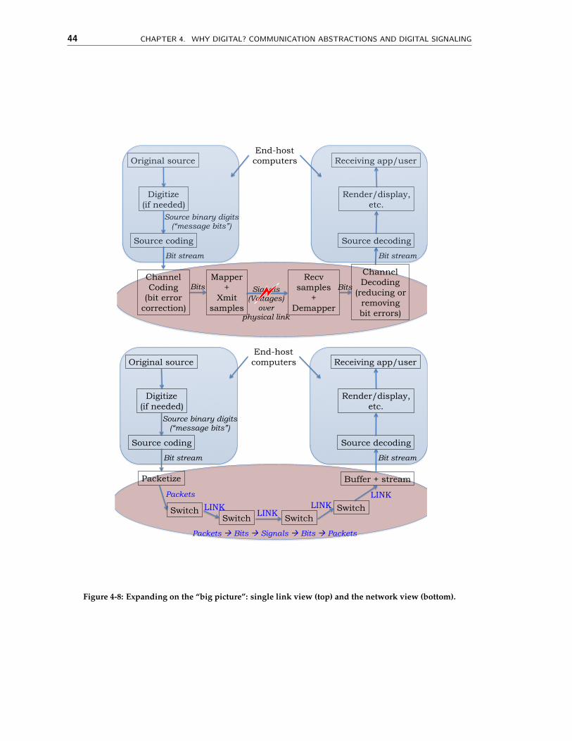
44 CHAPTER 4. WHY DIGITAL? COMMUNICATION ABSTRACTIONS AND DIGITAL SIGNALING
Digitize (if needed)
Original source
Source coding
Source binary digits (“message bits”)
Bit stream
Render/display, etc.
Receiving app/user
Source decoding
Bit stream
Channel Coding
(bit error correction)
Recv samples
+ Demapper
Mapper +
Xmit samples
Bits Signals (Voltages)
over physical link
Channel Decoding
(reducing or removing bit errors)
End-host computers
Bits
Digitize (if needed)
Original source
Source coding
Source binary digits (“message bits”)
Packets
Render/display, etc.
Receiving app/user
Source decoding
Bit stream
End-host computers
Packetize
Switch Switch Switch
Switch
Buffer + stream
LINK LINK LINK
LINK
Packets à Bits à Signals à Bits à Packets
Bit stream
Figure 4-8: Expanding on the “big picture”: single link view (top) and the network view (bottom).

MIT 6.02 DRAFT Lecture NotesLast update: October 14, 2011Comments, questions or bug reports?
Please contact hari at mit.edu
CHAPTER 5Coping with Bit Errors using Error
Correction Codes
Recall our main goal in designing digital communication networks: to send informationboth reliably and efficiently between nodes. Meeting that goal requires the use of tech-niques to combat bit errors, which are inevitable in both commmunication channels andstorage media.
The key idea we will apply to achieve reliable communication is the addition of redun-dancy to the transmitted data, to improve the probability that the original message can bereconstructed from the possibly corrupted data that is received. The sender has an encoderwhose job is to take the message and process it to produce the coded bits that are then sentover the channel. The receiver has a decoder whose job is to take the received (coded) bitsand to produce its best estimate of the message. The encoder-decoder procedures togetherconstitute channel coding; good channel codes provide error correction capabilities thatreduce the bit error rate (i.e., the probability of a bit error).
With proper design, full error correction may be possible, provided only a small num-ber of errors has occurred. Even when too many errors have occurred to permit correction,it may be possible to perform error detection. Error detection provides a way for the re-ceiver to tell (with high probability) if the message was decoded correctly or not. Errordetection usually works by the sender and receiver using a different code from the oneused to correct errors; common examples include the cyclic redundancy check (CRC) or hashfunctions. These codes take n-bit messages and produce a compact “signature” of that mes-sage that is much smaller than the message (e.g., the popular CRC-32 scheme produces a32-bit signature of an arbitrarily long message). The sender computes and transmits thesignature along with the message bits, usually appending it to the end of the message. Thereceiver, after running the decoder to correct errors, then computes the signature over itsestimate of the message bits and compares that signature to its estimate of the signaturebits in the received data. If the computed and estimated signatures are not equal, thenthe receiver considers the message to have one or more bit errors; otherwise, it assumesthat the message has been received correctly. This latter assumption is probabilistic: thereis some non-zero (though very small, for good signatures) probability that the estimatedand computed signatures match, but the receiver’s decoded message is different from the
45

46 CHAPTER 5. COPING WITH BIT ERRORS USING ERROR CORRECTION CODES
sender’s. If the signatures don’t match, the receiver and sender may use some higher-layerprotocol to arrange for the message to be retransmitted; we will study such schemes later.We will not study error detection codes like CRC or hash functions in this course.
Our plan for this chapter is as follows. To start, we will assume a binary symmetricchannel (BSC), which we defined and explained in the previous chapter; here the probabil-ity of a bit “flipping” is ε. Then, we will discuss and analyze a simple redundancy schemecalled a replication code, which will simply make n copies of any given bit. The replicationcode has a code rate of 1/n—that is, for every useful message bit, we end up transmittingn total bits. The overhead of the replication code of rate c is 1− 1/n, which is rather highfor the error correcting power of the code. We will then turn to the key ideas that allowus to build powerful codes capable of correcting errors without such a high overhead (orequivalently, capable of correcting far more errors at a given code rate compared to thereplication code).
There are two big, inter-related ideas used in essentially all error correction codes. Thefirst is the notion of embedding, where the messages one wishes to send are placed in ageometrically pleasing way in a larger space so that the distance between any two validpoints in the embedding is large enough to enable the correction and detection of errors.The second big idea is to use parity calculations, which are linear functions over the bitswe wish to send, to generate the redundancy in the bits that are actually sent. We willstudy examples of embeddings and parity calculations in the context of two classes ofcodes: linear block codes, which are an instance of the broad class of algebraic codes,and convolutional codes, which are perhaps the simplest instance of the broad class ofgraphical codes.
We start with a brief discussion of bit errors.
� 5.1 Bit Errors
A BSC is characterized by one parameter, ε, which we can assume to be < 1/2, the proba-bility of a bit error. It is a natural discretization of AWGN, which is also a single-parametermodel fully characterized by the variance, σ2. We can determine ε empirically by notingthat if we send N bits over the channel, the expected number of erroneously received bitsis N · ε. By sending a long known bit pattern and counting the fraction or erroneouslyreceived bits, we can estimate ε, thanks to the law of large numbers. In practice, even whenthe BSC is a reasonable error model, the range of ε could be rather large, between 10−2 (oreven a bit higher) all the way to 10−10 or even 10−12. A value of ε of about 10−2 means thatmessages longer than a 100 bits will see at least one error on average; given that the typicalunit of communication over a channel (a “packet”) is generally between 500 bits and 12000bits (or more, in some networks), such an error rate is too high.
But is a ε of 10−12 small enough that we don’t need to bother about doing any errorcorrection? The answer often depends on the data rate of the channel. If the channel hasa rate of 10 Gigabits/s (available today even on commodity server-class computers), thenthe “low” ε of 10−12 means that the receiver will see one error every 10 seconds on averageif the channel is continuously loaded. Unless we include some mechanisms to mitigatethe situation, the applications using the channel may find errors occurring too frequently.On the other hand, a ε of 10−12 may be fine over a communication channel running at 10

SECTION 5.2. THE SIMPLEST CODE: REPLICATION 47
Megabits/s, as long as there is some way to detect errors when they occur.The BSC is perhaps the simplest error model that is realistic, but real-world channels
exhibit more complex behaviors. For example, over many wireless and wired channelsas well as on storage media (like CDs, DVDs, and disks), errors can occur in bursts. Thatis, the probability of any given bit being received wrongly depends on recent history: theprobability is higher if the bits in the recent past were received incorrectly. Our goal is todevelop techniques to mitigate the effects of both the BSC and burst errors. We’ll start withtechniques that work well over a BSC and then discuss how to deal with bursts.
� 5.2 The Simplest Code: Replication
In general, a channel code provides a way to map message words to codewords (analogousto a source code, except here the purpose is not compression but rather the addition ofredundancy for error correction or detection). In a replication code, each bit b is encodedas n copies of b, and the result is delivered. If we consider bit b to be the message word,then the corresponding codeword is bn (i.e., bb...b, n times). In this example, there are onlytwo possible message words (0 and 1) and two corresponding codewords. The replicationcode is absurdly simple, yet it’s instructive and sometimes even useful in practice!
But how well does it correct errors? To answer this question, we will write out theprobability of overcoming channel errors for the BSC error model with the replication code.That is, if the channel corrupts each bit with probability ε, what is the probability that thereceiver decodes the received codeword correctly to produce the message word that wassent?
The answer depends on the decoding method used. A reasonable decoding method ismaximum likelihood decoding: given a received codeword, r, which is some n-bit combina-tion of 0’s and 1’s, the decoder should produce the most likely message that could havecaused r to be received. Since the BSC error probability, ε, is smaller than 1/2, the mostlikely option is the codeword that has the most number of bits in common with r. Thisdecoding rule results in the minimum probability of error when all messages are equallylikely.
Hence, the decoding process is as follows. First, count the number of 1’s in r. If there aremore than c/2 1’s, then decode the message as 1. If there are more than c/2 0’s, then decodethe message as 0. When c is odd, each codeword will be decoded unambiguously. Whenc is even, and has an equal number of 0’s and 1’s, the decoder can’t really tell whether themessage was a 0 or 1, and the best it can do is to make an arbitrary decision. (We havetacitly assumed that the a priori probability of sending a message 0 is the same as that ofsending a 1.)
We can write the probability of decoding error for the replication code as follows, beinga bit careful with the limits of the summation:
P(decoding error) =
{∑
ni=d n
2 e(n
i
)εi(1− ε)n−i if n odd
∑ni= n
2 +1
(ni
)εi(1− ε)n−i + 1
2
( nn/2
)εn/2(1− ε)n/2 if n even
(5.1)
The notation(n
i
)denotes the number of ways of selecting i objects (in this case, bit posi-
tions) from n objects.

48 CHAPTER 5. COPING WITH BIT ERRORS USING ERROR CORRECTION CODES
Figure 5-1: Probability of a decoding error with the replication code that replaces each bit b with n copiesof b. The code rate is 1/n.
When n is even, we add a term at the end to account for the fact that the decoder has afifty-fifty chance of guessing correctly when it receives a codeword with an equal numberof 0’s and 1’s.
Figure 5-1 shows the probability of decoding error as a function of the replication factor,n, for the replication code, computed using Equation (5.1). The y-axis is on a log scale, andthe probability of error is more or less a straight line with negative slope (if you ignorethe flat pieces), which means that the decoding error probability decreases exponentiallywith the code rate. It is also worth noting that the error probability is the same whenn = 2` as when n = 2`− 1. The reason, of course, is that the decoder obtains no additionalinformation that it already didn’t know from any 2`− 1 of the received bits.
Despite the exponential reduction in the probability of decoding error as n increases,the replication code is extremely inefficient in terms of the overhead it incurs, for a givenrate, 1/n. As such, it is used only in situations when bandwidth is plentiful and there isn’tmuch computation time to implement a more complex decoder.
We now turn to developing more sophisticated codes. There are two big related ideas:embedding messages into spaces in a way that achieves structural separation and parity (linear)computations over the message bits.
� 5.3 Embeddings and Hamming Distance
Let’s start our investigation into error correction by examining the situations in whicherror detection and correction are possible. For simplicity, we will focus on single-errorcorrection (SEC) here. By that we mean codes that are guaranteed to produce the correctmessage word, given a received codeword with zero or one bit errors in it. If the received

SECTION 5.3. EMBEDDINGS AND HAMMING DISTANCE 49
Figure 5-2: Codewords separated by a Hamming distance of 2 can be used to detect single bit errors. Thecodewords are shaded in each picture. The picture on the left is a (2,1) repetition code, which maps 1-bitmessages to 2-bit codewords. The code on the right is a (3,2) code, which maps 2-bit messages to 3-bitcodewords.
codeword has more than one bit error, then we can make no guarantees (the method mightreturn the correct message word, but there is at least one instance where it will return thewrong answer).
There are 2n possible n-bit strings. Define the Hamming distance (HD) between two n-bit words, w1 and w2, as the number of bit positions in which the messages differ. Thus0 ≤HD(w1, w2) ≤ n.
Suppose that HD(w1, w2) = 1. Consider what happens if we transmit w1 and there’sa single bit error that inconveniently occurs at the one bit position in which w1 and w2
differ. From the receiver’s point of view it just received w2—the receiver can’t detect thedifference between receiving w1 with a unfortunately placed bit error and receiving w2.In this case, we cannot guarantee that all single bit errors will be corrected if we choose acode where w1 and w2 are both valid codewords.
What happens if we increase the Hamming distance between any two valid codewordsto 2? More formally, let’s restrict ourselves to only sending some subset S = {w1, w2, ..., ws}of the 2n possible words such that
HD(wi, w j) ≥ 2 for all wi, w j ∈ S where i 6= j (5.2)
Thus if the transmission of wi is corrupted by a single error, the result is not an elementof S and hence can be detected as an erroneous reception by the receiver, which knowswhich messages are elements of S. A simple example is shown in Figure 5-2: 00 and 11 arevalid codewords, and the receptions 01 and 10 are surely erroneous.
We define the minimum Hamming distance of a code as the minimum Hamming distancebetween any two codewords in the code. From the discussion above, it should be easy tosee what happens if we use a code whose minimum Hamming distance is D. We state theproperty formally:
Theorem 5.1 A code with a minimum Hamming distance of D can detect any error pattern ofD− 1 or fewer errors. Moreover, there is at least one error pattern with D errors that cannot bedetected reliably.

50 CHAPTER 5. COPING WITH BIT ERRORS USING ERROR CORRECTION CODES
Hence, if our goal is to detect errors, we can use an embedding of the set of messages wewish to transmit into a bigger space, so that the minimum Hamming distance between anytwo codewords in the bigger space is at least one more than the number of errors we wishto detect. (We will discuss how to produce such embeddings in the subsequent sections.)
But what about the problem of correcting errors? Let’s go back to Figure 5-2, with S ={00,11}. Suppose the received sequence is 01. The receiver can tell that a single error hasoccurred, but it can’t tell whether the correct data sent was 00 or 11—both those possiblepatterns are equally likely under the BSC error model.
Ah, but we can extend our approach by producing an embedding with more spacebetween valid codewords! Suppose we limit our selection of messages in S even further,as follows:
HD(wi, w j) ≥ 3 for all wi, w j ∈ S where i 6= j (5.3)
How does it help to increase the minimum Hamming distance to 3? Let’s define onemore piece of notation: let Ewi be the set of messages resulting from corrupting wi with asingle error. For example, E000 = {001,010,100}. Note that HD(wi,an element of Ewi ) = 1.
With a minimum Hamming distance of 3 between the valid codewords, observe thatthere is no intersection between Ewi and Ew j when i 6= j. Why is that? Suppose therewas a message wk that was in both Ewi and Ew j . We know that HD(wi, wk) = 1 andHD(w j, wk) = 1, which implies that wi and w j differ in at most two bits and consequentlyHD(wi, w j) ≤ 2. (This result is an application of Theorem 5.2 below, which states that theHamming distance satisfies the triangle inequality.) That contradicts our specification thattheir minimum Hamming distance be 3. So the Ewi don’t intersect.
So now we can correct single bit errors as well: the received message is either a memberof S (no errors), or is a member of some particular Ewi (one error), in which case the receivercan deduce the original message was wi. Here’s another simple example: let S = {000,111}.So E000 = {001,010,100} and E111 = {110,101,011} (note that E000 doesn’t intersect E111).Suppose the received sequence is 101. The receiver can tell there has been a single errorbecause 101 /∈ S. Moreover it can deduce that the original message was most likely 111because 101 ∈ E111.
We can formally state some properties from the above discussion, and specify the error-correcting power of a code whose minimum Hamming distance is D.
Theorem 5.2 The Hamming distance between n-bit words satisfies the triangle inequality. Thatis, HD(x, y) + HD(y, z) ≥ HD(x, z).
Theorem 5.3 For a BSC error model with bit error probability < 1/2, the maximum likelihood de-coding strategy is to map any received word to the valid codeword with smallest Hamming distancefrom the received one (ties may be broken arbitrarily).
Theorem 5.4 A code with a minimum Hamming distance of D can correct any error pattern ofbD−1
2 c or fewer errors. Moreover, there is at least one error pattern with bD−12 c+ 1 errors that
cannot be corrected reliably.
Equation (5.3) gives us a way of determining if single-bit error correction can alwaysbe performed on a proposed set S of transmission messages—we could write a programto compute the Hamming distance between all pairs of messages in S and verify that the

SECTION 5.4. LINEAR BLOCK CODES AND PARITY CALCULATIONS 51
minimum Hamming distance was at least 3. We can also easily generalize this idea tocheck if a code can always correct more errors. And we can use the observations madeabove to decode any received word: just find the closest valid codeword to the receivedone, and then use the known mapping between each distinct message and the codewordto produce the message. The message will be the correct one if the actual number of errorsis no larger than the number for which error correction is guaranteed. The check for thenearest codeword may be exponential in the number of message bits we would like tosend, making it a reasonable approach only if the number of bits is small.
But how do we go about finding a good embedding (i.e., good code words)? This taskisn’t straightforward, as the following example shows. Suppose we want to reliably send4-bit messages so that the receiver can correct all single-bit errors in the received words.Clearly, we need to find a set of messages S with 24 elements. What should the membersof S be?
The answer isn’t obvious. Once again, we could write a program to search throughpossible sets of n-bit messages until it finds a set of size 16 with a minimum Hammingdistance of 3. An exhaustive search shows that the minimum n is 7, and one example of Sis:
0000000 1100001 1100110 00001110101010 1001011 1001100 01011011010010 0110011 0110100 10101011111000 0011001 0011110 1111111
But such exhaustive searches are impractical when we want to send even modestlylonger messages. So we’d like some constructive technique for building S. Much of thetheory and practice of coding is devoted to finding such constructions and developingefficient encoding and decoding strategies.
Broadly speaking, there are two classes of code constructions, each with an enormousnumber of example instances. The first is the class of algebraic block codes. The secondis the class of graphical codes. We will study two simple examples of linear block codes,which themselves are a sub-class of algebraic block codes: rectangular parity codes andHamming codes. We also note that the replication code discussed in Section 5.2 is anexample of a linear block code.
In the next two chapters, we will study convolutional codes, a sub-class of graphicalcodes.
� 5.4 Linear Block Codes and Parity Calculations
Linear block codes are examples of algebraic block codes, which take the set of k-bit mes-sages we wish to send (there are 2k of them) and produce a set of 2k codewords, each n bitslong (n ≥ k) using algebraic operations over the block. The word “block” refers to the factthat any long bit stream can be broken up into k-bit blocks, which are each then expandedto produce n-bit codewords that are sent.
Such codes are also called (n, k) codes, where k message bits are combined to producen code bits (so each codeword has n− k “redundancy” bits). Often, we use the notation(n, k, d), where d refers to the minimum Hamming distance of the block code. The rate of a

52 CHAPTER 5. COPING WITH BIT ERRORS USING ERROR CORRECTION CODES
block code is defined as k/n; the larger the rate, the less the redundancy overhead incurredby the code.
A linear code (whether a block code or not) produces codewords from message bits byrestricting the algebraic operations to linear functions over the message bits. By linear, wemean that any given bit in a valid codeword is computed as the weighted sum of one ormore original message bits.
Linear codes, as we will see, are both powerful and efficient to implement. They arewidely used in practice. In fact, all the codes we will study—including convolutionalcodes—are linear, as are most of the codes widely used in practice. We already lookedat the properties of a simple linear block code: the replication code we discussed in Sec-tion 5.2 is a linear block code with parameters (n,1, n).
An important and popular class of linear codes are binary linear codes. The computationsin the case of a binary code use arithmetic modulo 2, which has a special name: algebrain a Galois Field of order 2, also denoted F2. A field must define rules for addition andmultiplication, and their inverses. Addition in F2 is according to the following rules: 0 +0 = 1 + 1 = 0; 1 + 0 = 0 + 1 = 1. Multiplication is as usual: 0 · 0 = 0 · 1 = 1 · 0 = 0; 1 · 1 = 1.We leave you to figure out the additive and multiplicative inverses of 0 and 1. Our focusin this book will be on linear codes over F2, but there are natural generalizations to fieldsof higher order (in particular, Reed Solomon codes, which are over Galois Fields of order2q).
A linear code is characterized by the following theorem, which is both a necessary anda sufficient condition for a code to be linear:
Theorem 5.5 A code is linear if, and only if, the sum of any two codewords is another codeword.
For example, the block code defined by codewords 000,101,011 is not a linear code,because 101 + 011 = 110 is not a codeword. But if we add 110 to the set, we get a lin-ear code because the sum of any two codewords is now another codeword. The code000,101,011,110 has a minimum Hamming distance of 2 (that is, the smallest Hammingdistance between any two codewords in 2), and can be used to detect all single-bit errorsthat occur during the transmission of a code word. You can also verify that the minimumHamming distance of this code is equal to the smallest number of 1’s in a non-zero code-word. In fact, that’s a general property of all linear block codes, which we state formallybelow:
Theorem 5.6 Define the weight of a codeword as the number of 1’s in the word. Then, the mini-mum Hamming distance of a linear block code is equal to the weight of the non-zero codeword withthe smallest weight.
To see why, use the property that the sum of any two codewords must also be a code-word, and that the Hamming distance between any two codewords is equal to the weightof their sum (i.e., weight(u + v) = HD(u, v)). (In fact, the Hamming distance between anytwo bit-strings of equal length is equal to the weight of their sum.) We leave the completeproof of this theorem as a useful and instructive exercise for the reader.
The rest of this section shows how to construct linear block codes over F2. For simplicity,and without much loss of generality, we will focus on correcting single-bit errors. i.e.,on single-error correction (SEC) codes.. We will show two ways of building the set S of

SECTION 5.4. LINEAR BLOCK CODES AND PARITY CALCULATIONS 53
transmission messages to have single-error correction capability, and will describe howthe receiver can perform error correction on the (possibly corrupted) received messages.
We will start with the rectangular parity code in Section 5.4.1, and then discuss the clev-erer and more efficient Hamming code in Section 5.4.3.
� 5.4.1 Rectangular Parity SEC Code
We define the parity of bits x1, x2, . . . , xn as (x1 + x2 + . . . + xn), where the addition is per-formed modulo 2 (it’s the same as taking the exclusive OR of the n bits). The parity is evenwhen the sum is 0 (i.e., the number of ones is even), and odd otherwise.
Let parity(s) denote the parity of all the bits in the bit-string s. We’ll use a dot, ·, toindicate the concatenation (sequential joining) of two messages or a message and a bit. Forany message M (a sequence of one or more bits), let w = M · parity(M). You should beable to confirm that parity(w) = 0. This code, which adds a parity bit to each message,is also called the even parity code, because the number of ones in each codeword is even.Even parity lets us detect single errors because the set of codewords, {w}, each defined asM · parity(M), has a Hamming distance of 2.
If we transmit w when we want to send some message M, then the receiver can take thereceived word, r, and compute parity(r) to determine if a single error has occurred. Thereceiver’s parity calculation returns 1 if an odd number of the bits in the received messagehas been corrupted. When the receiver’s parity calculation returns a 1, we say there hasbeen a parity error.
This section describes a simple approach to building an SEC code by constructing mul-tiple parity bits, each over various subsets of the message bits, and then using the resultingparity errors (or non-errors) to help pinpoint which bit was corrupted.
Rectangular code construction: Suppose we want to send a k-bit message M. Shape thek bits into a rectangular array with r rows and c columns, i.e., k = rc. For example, ifk = 8, the array could be 2× 4 or 4× 2 (or even 8× 1 or 1× 8, though those are a little lessinteresting). Label each data bit with a subscript giving its row and column: the first bitwould be d11, the last bit drc. See Figure 5-3.
Define p row(i) to be the parity of all the bits in row i of the array and let R be all therow parity bits collected into a sequence:
R = [p row(1),p row(2), . . . ,p row(r)]
Similarly, define p col( j) to be the parity of all the bits in column j of the array and let C beall the column parity bits collected into a sequence:
C = [p col(1),p col(2), . . . ,p col(c)]
Figure 5-3 shows what we have in mind when k = 8.Let w = M · R · C, i.e., the transmitted codeword consists of the original message M,
followed by the row parity bits R in row order, followed by the column parity bits C incolumn order. The length of w is n = rc + r + c. This code is linear because all the paritybits are linear functions of the message bits. The rate of the code is rc/(rc + r + c).
We now prove that the rectangular parity code can correct all single-bit errors.

54 CHAPTER 5. COPING WITH BIT ERRORS USING ERROR CORRECTION CODES
d11 d12 d13 d14 p row(1)d21 d22 d23 d24 p row(2)
p col(1) p col(2) p col(3) p col(4)
Figure 5-3: A 2× 4 arrangement for an 8-bit message with row and column parity.
0 1 1 0 01 1 0 1 11 0 1 1
(a)
1 0 0 1 10 0 1 0 11 0 1 0
(b)
0 1 1 1 11 1 1 0 11 0 0 0
(c)
Figure 5-4: Example received 8-bit messages. Which, if any, have one error? Which, if any, have two?
Proof of single-error correction property: This rectangular code is an SEC code for allvalues of r and c. We will show that it can correct all single bit errors by showing that itsminimum Hamming distance is 3 (i.e., the Hamming distance between any two codewordsis at least 3). Consider two different uncoded messages, Mi and M j. There are three casesto discuss:
• If Mi and M j differ by a single bit, then the row and column parity calculationsinvolving that bit will result in different values. Thus, the corresponding codewords,wi and w j, will differ by three bits: the different data bit, the different row parity bit,and the different column parity bit. So in this case HD(wi, w j) = 3.
• If Mi and M j differ by two bits, then either (1) the differing bits are in the samerow, in which case the row parity calculation is unchanged but two column paritycalculations will differ, (2) the differing bits are in the same column, in which case thecolumn parity calculation is unchanged but two row parity calculations will differ,or (3) the differing bits are in different rows and columns, in which case there will betwo row and two column parity calculations that differ. So in this case HD(wi, w j) ≥4.
• If Mi and M j differ by three or more bits, then HD(wi, w j) ≥ 3 because wi and w jcontain Mi and M j respectively.
Hence we can conclude that HD(wi, w j) ≥ 3 and our simple “rectangular” code will beable to correct all single-bit errors.
Decoding the rectangular code: How can the receiver’s decoder correctly deduce Mfrom the received w, which may or may not have a single bit error? (If w has more thanone error, then the decoder does not have to produce a correct answer.)
Upon receiving a possibly corrupted w, the receiver checks the parity for the rows andcolumns by computing the sum of the appropriate data bits and the corresponding paritybit (all arithmetic in F2). This sum will be 1 if there is a parity error. Then:
• If there are no parity errors, then there has not been a single error, so the receiver canuse the data bits as-is for M. This situation is shown in Figure 5-4(a).

SECTION 5.4. LINEAR BLOCK CODES AND PARITY CALCULATIONS 55
Figure 5-5: A codeword in systematic form for a block code. Any linear code can be transformed into anequivalent systematic code.
• If there is single row or column parity error, then the corresponding parity bit is inerror. But the data bits are okay and can be used as-is for M. This situation is shownin Figure 5-4(c), which has a parity error only in the fourth column.
• If there is one row and one column parity error, then the data bit in that row andcolumn has an error. The decoder repairs the error by flipping that data bit and thenuses the repaired data bits for M. This situation is shown in Figure 5-4(b), wherethere are parity errors in the first row and fourth column indicating that d14 shouldbe flipped to be a 0.
• Other combinations of row and column parity errors indicate that multiple errorshave occurred. There’s no “right” action the receiver can undertake because itdoesn’t have sufficient information to determine which bits are in error. A commonapproach is to use the data bits as-is for M. If they happen to be in error, that will bedetected by the error detection code (mentioned near the beginning of this chapter).
This recipe will produce the most likely message, M, from the received codeword if therehas been at most a single transmission error.
In the rectangular code the number of parity bits grows at least as fast as√
k (it shouldbe easy to verify that the smallest number of parity bits occurs when the number of rows,r, and the number of columns, c, are equal). Given a fixed amount of communication“bandwidth” or resource, we’re interested in devoting as much of it as possible to sendingmessage bits, not parity bits. Are there other SEC codes that have better code rates thanour simple rectangular code? A natural question to ask is: how little redundancy can we getaway with and still manage to correct errors?
The Hamming code uses a clever construction that uses the intuition developed whileanswering the question mentioned above. We answer this question next.
� 5.4.2 How many parity bits are needed in an SEC code?
Let’s think about what we’re trying to accomplish with an SEC code: the correction oftransmissions that have a single error. For a transmitted message of length n there aren + 1 situations the receiver has to distinguish between: no errors and a single error ina specified position along the string of n received bits. Then, depending on the detectedsituation, the receiver can make, if necessary, the appropriate correction.
Our first observation, which we will state here without proof, is that any linear codecan be transformed into an equivalent systematic code. A systematic code is one where

56 CHAPTER 5. COPING WITH BIT ERRORS USING ERROR CORRECTION CODES
every n-bit codeword can be represented as the original k-bit message followed by then− k parity bits (it actually doesn’t matter how the original message bits and parity bitsare interspersed). Figure 5-5 shows a codeword in systematic form.
So, given a systematic code, how many parity bits do we absolutely need? We needto choose n so that single error correction is possible. Since there are n − k parity bits,each combination of these bits must represent some error condition that we must be ableto correct (or infer that there were no errors). There are 2n−k possible distinct parity bitcombinations, which means that we can distinguish at most that many error conditions.We therefore arrive at the constraint
n + 1 ≤ 2n−k (5.4)
i.e., there have to be enough parity bits to distinguish all corrective actions that mightneed to be taken (including no action). Given k, we can determine n− k, the number ofparity bits needed to satisfy this constraint. Taking the log (to base 2) of both sides, wecan see that the number of parity bits must grow at least logarithmically with the numberof message bits. Not all codes achieve this minimum (e.g., the rectangular code doesn’t),but the Hamming code, which we describe next, does.
We also note that the reasoning here for an SEC code can be extended to determine alower bound on the number of parity buts needed to correct t > 1 errors.
� 5.4.3 Hamming Codes
Intuitively, it makes sense that for a code to be efficient, each parity bit should protectas many data bits as possible. By symmetry, we’d expect each parity bit to do the sameamount of ”work” in the sense that each parity bit would protect the same number of databits. If some parity bit is shirking its duties, it’s likely we’ll need a larger number of paritybits in order to ensure that each possible single error will produce a unique combinationof parity errors (it’s the unique combinations that the receiver uses to deduce which bit, ifany, had an error).
The class of Hamming single error correcting codes is noteworthy because they areparticularly efficient in the use of parity bits: the number of parity bits used by Hammingcodes grows logarithmically with the size of the codeword. Figure 5-6 shows two examplesof the class: the (7,4) and (15,11) Hamming codes. The (7,4) Hamming code uses 3 paritybits to protect 4 data bits; 3 of the 4 data bits are involved in each parity computation. The(15,11) Hamming code uses 4 parity bits to protect 11 data bits, and 7 of the 11 data bits areused in each parity computation (these properties will become apparent when we discussthe logic behind the construction of the Hamming code in Section 5.4.4).
Looking at the diagrams, which show the data bits involved in each parity computation,you should convince yourself that each possible single error (don’t forget errors in one ofthe parity bits!) results in a unique combination of parity errors. Let’s work through theargument for the (7,4) Hamming code. Here are the parity-check computations performed

SECTION 5.4. LINEAR BLOCK CODES AND PARITY CALCULATIONS 57
d1 p1 p2
p3
d2 d3
d4
(a) (7,4) code
d1 p1 p2
p3
d2 d3
d4
p4
d9
d11
d10
d6
d7 d5
d8
(b) (15,11) code
Figure 5-6: Venn diagrams of Hamming codes showing which data bits are protected by each parity bit.
by the receiver:
E1 = (d1 + d2 + d4 + p1) mod 2
E2 = (d1 + d3 + d4 + p2) mod 2
E3 = (d2 + d3 + d4 + p3) mod 2
where each Ei is called a syndrome bit because it helps the receiver diagnose the “illness”(errors) in the received data. For each combination of syndrome bits, we can look forthe bits in each codeword that appear in all the Ei computations that produced 1; thesebits are potential candidates for having an error since any of them could have caused theobserved parity errors. Now eliminate from the candidates those bits that appear in any Eicomputations that produced 0 since those calculations prove those bits didn’t have errors.We’ll be left with either no bits (no errors occurred) or one bit (the bit with the single error).
For example, if E1 = 1, E2 = 0 and E3 = 1, we notice that bits d2 and d4 both appearin the computations for E1 and E3. However, d4 appears in the computation for E2 andshould be eliminated, leaving d2 as the sole candidate as the bit with the error.
Another example: suppose E1 = 1, E2 = 0 and E3 = 0. Any of the bits appearing in thecomputation for E1 could have caused the observed parity error. Eliminating those thatappear in the computations for E2 and E3, we’re left with p1, which must be the bit withthe error.
Applying this reasoning to each possible combination of parity errors, we can make atable that shows the appropriate corrective action for each combination of the syndromebits:

58 CHAPTER 5. COPING WITH BIT ERRORS USING ERROR CORRECTION CODES
E3E2E1 Corrective Action000 no errors001 p1 has an error, flip to correct010 p2 has an error, flip to correct011 d1 has an error, flip to correct100 p3 has an error, flip to correct101 d2 has an error, flip to correct110 d3 has an error, flip to correct111 d4 has an error, flip to correct
� 5.4.4 Is There a Logic to the Hamming Code Construction?
So far so good, but the allocation of data bits to parity-bit computations may seem ratherarbitrary and it’s not clear how to build the corrective action table except by inspection.
The cleverness of Hamming codes is revealed if we order the data and parity bits in acertain way and assign each bit an index, starting with 1:
index 1 2 3 4 5 6 7binary index 001 010 011 100 101 110 111
(7,4) code p1 p2 d1 p3 d2 d3 d4
This table was constructed by first allocating the parity bits to indices that are powersof two (e.g., 1, 2, 4, . . . ). Then the data bits are allocated to the so-far unassigned indicies,starting with the smallest index. It’s easy to see how to extend this construction to anynumber of data bits, remembering to add additional parity bits at indices that are a powerof two.
Allocating the data bits to parity computations is accomplished by looking at their re-spective indices in the table above. Note that we’re talking about the index in the table, notthe subscript of the bit. Specifically, di is included in the computation of p j if (and only if)the logical AND of binary index(di) and binary index(p j) is non-zero. Put another way, diis included in the computation of p j if, and only if, index(p j) contributes to index(di) whenwriting the latter as sums of powers of 2.
So the computation of p1 (with an index of 1) includes all data bits with odd indices: d1,d2 and d4. And the computation of p2 (with an index of 2) includes d1, d3 and d4. Finally,the computation of p3 (with an index of 4) includes d2, d3 and d4. You should verify thatthese calculations match the Ei equations given above.
If the parity/syndrome computations are constructed this way, it turns out that E3E2E1,treated as a binary number, gives the index of the bit that should be corrected. For exam-ple, if E3E2E1 = 101, then we should correct the message bit with index 5, i.e., d2. Thiscorrective action is exactly the one described in the earlier table we built by inspection.
The Hamming code’s syndrome calculation and subsequent corrective action can be ef-ficiently implemented using digital logic and so these codes are widely used in contextswhere single error correction needs to be fast, e.g., correction of memory errors when fetch-ing data from DRAM.

SECTION 5.5. PROTECTING LONGER MESSAGES WITH SEC CODES 59
Figure 5-7: Dividing a long message into multiple SEC-protected blocks of k bits each, adding parity bitsto each constituent block. The red vertical rectangles refer to bit errors.
� 5.5 Protecting Longer Messages with SEC Codes
SEC codes are a good building block, but they correct at most one error in a block of ncoded bits. As messages get longer, the solution, of course, is to break up a longer messageinto smaller blocks of k bits each, and to protect each one with its own SEC code. The resultmight look as shown in Figure 5-7.
� 5.5.1 Coping with Burst Errors
Over many channels, errors occur in bursts and the BSC error model is invalid. For ex-ample, wireless channels suffer from interference from other transmitters and from fading,caused mainly by multi-path propagation when a given signal arrives at the receiver frommultiple paths and interferes in complex ways because the different copies of the signalexperience different degrees of attenuation and different delays. Another reason for fad-ing is the presence of obstacles on the path between sender and receiver; such fading iscalled shadow fading.
The behavior of a fading channel is complicated and beyond the scope of 6.02, but theimpact of fading on communication is that the random process describing the bit errorprobability is no longer independent and identically distributed from one bit to another.The BSC model needs to be replaced with a more complicated one in which errors mayoccur in bursts. Many such theoretical models guided by empirical data exist, but we won’tgo into them here. Our goal is to understand how to develop error correction mechanismswhen errors occur in bursts.
But what do we mean by a “burst”? The simplest model is to model the channel ashaving two states, a “good” state and a “bad” state. In the “good” state, the bit errorprobability is pg and in the “bad” state, it is pb > pg. Once in the good state, the channelhas some probability of remaining there (generally > 1/2) and some probability of movinginto the “bad” state, and vice versa. It should be easy to see that this simple model hasthe property that the probability of a bit error depends on whether the previous bit (orprevious few bits) are in error or not. The reason is that the odds of being in a “good” stateare high if the previous few bits have been correct.
At first sight, it might seem like the SEC schemes we studied are poorly suited for a

60 CHAPTER 5. COPING WITH BIT ERRORS USING ERROR CORRECTION CODES
Figure 5-8: Interleaving can help recover from burst errors: code each block row-wise with an SEC, buttransmit them in interleaved fashion in columnar order. As long as a set of burst errors corrupts some setof kth bits, the receiver can recover from all the errors in the burst.
channel experiencing burst errors. The reason is shown in Figure 5-8 (left), where eachblock of the message is protected by its SEC parity bits. The different blocks are shown asdifferent rows. When a burst error occurs, multiple bits in an SEC block are corrupted, andthe SEC can’t recover from them.
Interleaving is a commonly used technique to recover from burst errors on a channeleven when the individual blocks are protected with a code that, on the face of it, is notsuited for burst errors. The idea is simple: code the blocks as before, but transmit them ina “columnar” fashion, as shown in Figure 5-8 (right). That is, send the first bit of block 1,then the first bit of block 2, and so on until all the first bits of each block in a set of somepredefined size are sent. Then, send the second bits of each block in sequence, then thethird bits, and so on.
What happens on a burst error? Chances are that it corrupts a set of “first” bits, or aset of “second” bits, or a set of “third” bits, etc., because those are the bits sent in order onthe channel. As long as only a set of kth bits are corrupted, the receiver can correct all theerrors. The reason is that each coded block will now have at most one error. Thus, SECcodes are a useful primitive to correct against burst errors, in concert with interleaving.
� Acknowledgments
Many thanks to Katrina LaCurts for carefully reading these notes and making several use-ful comments.

SECTION 5.5. PROTECTING LONGER MESSAGES WITH SEC CODES 61
� Problems and Questions
1. Prove that the Hamming distance satisfies the triangle inequality. That is, show thatHD(x, y) + HD(y, z) ≥HD(x, z) for any three n-bit binary words.
2. Consider the following rectangular linear block code:
D0 D1 D2 D3 D4 | P0D5 D6 D7 D8 D9 | P1D10 D11 D12 D13 D14 | P2-------------------------P3 P4 P5 P6 P7 |
Here, D0–D14 are data bits, P0–P2 are row parity bits and P3–P7 are column paritybits. What are n, k, and d for this linear code?
3. Consider a rectangular parity code as described in Section 5.4.1. Ben Bitdiddle wouldlike use this code at a variety of different code rates and experiment with them onsome channel.
(a) Is it possible to obtain a rate lower than 1/3 with this code? Explain your an-swer.
(b) Suppose he is interested in code rates like 1/2, 2/3, 3/4, etc.; i.e., in general arate of n−1
n , for integer n > 1. Is it always possible to pick the parameters ofthe code (i.e, the block size and the number of rows and columns over which toconstruct the parity bits) so that any such code rate is achievable? Explain youranswer.
4. Two-Bit Communications (TBC), a slightly suspect network provider, uses the fol-lowing linear block code over its channels. All arithmetic is in F2.
P0 = D0, P1 = (D0 + D1), P2 = D1.
(a) What are n and k for this code?
(b) Suppose we want to perform syndrome decoding over the received bits. Writeout the three syndrome equations for E0, E1, E2.
(c) For the eight possible syndrome values, determine what error can be detected(none, error in a particular data or parity bit, or multiple errors). Make yourchoice using maximum likelihood decoding, assuming a small bit error prob-ability (i.e., the smallest number of errors that’s consistent with the given syn-drome).
(d) Suppose that the the 5-bit blocks arrive at the receiver in the following order:D0, D1, P0, P1, P2. If 11011 arrives, what will the TBC receiver report as the re-ceived data after error correction has been performed? Explain your answer.
(e) TBC would like to improve the code rate while still maintaining single-bit errorcorrection. Their engineer would like to reduce the number of parity bits by 1.Give the formulas for P0 and P1 that will accomplish this goal, or briefly explainwhy no such code is possible.

62 CHAPTER 5. COPING WITH BIT ERRORS USING ERROR CORRECTION CODES
5. Pairwise Communications has developed a linear block code over F2 with three dataand three parity bits, which it calls the pairwise code:
P1 = D1 + D2 (Each Di is a data bit; each Pi is a parity bit.)
P2 = D2 + D3
P3 = D3 + D1
(a) Fill in the values of the following three attributes of this code:(i) Code rate =(ii) Number of 1s in a minimum-weight non-zero codeword =(iii) Minimum Hamming distance of the code =
6. Consider the same “pairwise code” as in the previous problem. The receiver com-putes three syndrome bits from the (possibly corrupted) received data and paritybits: E1 = D1 + D2 + P1, E2 = D2 + D3 + P2, and E3 = D3 + D1 + P3. The receiverperforms maximum likelihood decoding using the syndrome bits. For the combi-nations of syndrome bits in the table below, state what the maximum-likelihood de-coder believes has occured: no errors, a single error in a specific bit (state which one),or multiple errors.
E3E2E1 Error pattern [No errors / Error in bit ... (specify bit) / Multiple errors]
0 0 00 0 10 1 00 1 11 0 01 0 11 1 01 1 1
7. Alyssa P. Hacker extends the aforementioned pairwise code by adding an overall par-ity bit. That is, she computes P4 = ∑
3i=1(Di + Pi), and appends P4 to each original code-
word to produce the new set of codewords. What improvement in error correctionor detection capabilities, if any, does Alyssa’s extended code show over Pairwise’soriginal code? Explain your answer.
8. For each of the sets of codewords below, determine whether the code is a linear blockcode over F2 or not. Also give the rate of each code.
(a) {000,001,010,011}.(b) {000, 011, 110, 101}.(c) {111, 100, 001, 010}.(d) {00000, 01111, 10100, 11011}.(e) {00000}.

SECTION 5.5. PROTECTING LONGER MESSAGES WITH SEC CODES 63
9. For any linear block code over F2 with minimum Hamming distance at least 2t + 1between codewords, show that:
2n−k ≥ 1 +(
n1
)+
(n2
)+ . . .
(nt
).
Hint: How many errors can such a code always correct?
10. For each (n, k, d) combination below, state whether a linear block code with thoseparameters exists or not. Please provide a brief explanation for each case: if such acode exists, give an example; if not, you may rely on a suitable necessary condition.
(a) (31,26,3): Yes / No
(b) (32,27,3): Yes / No
(c) (43,42,2): Yes / No
(d) (27,18,3): Yes / No
(e) (11,5,5): Yes / No
11. Using the Hamming code construction for the (7,4) code, construct the parity equa-tions for the (15,11) code. How many equations does this code have? How manymessage bits contribute to each parity bit?
12. Prove Theorems 5.2 and 5.3. (Don’t worry too much if you can’t prove the latter; wewill give the proof when we discuss convolutional codes in Lecture 8.)
13. The weight of a codeword in a linear block code over F2 is the number of 1’s inthe word. Show that any linear block code must either: (1) have only even weightcodewords, or (2) have an equal number of even and odd weight codewords.Hint: Proof by contradiction.
14. There are N people in a room, each wearing a hat colored red or blue, standing in aline in order of increasing height. Each person can see only the hats of the people infront, and does not know the color of his or her own hat. They play a game as a team,whose rules are simple. Each person gets to say one word: “red” or “blue”. If theword they say correctly guesses the color of their hat, the team gets 1 point; if theyguess wrong, 0 points. Before the game begins, they can get together to agree on aprotocol (i.e., what word they will say under what conditions). Once they determinethe protocol, they stop talking, form the line, and are given their hats at random.
Can you develop a protocol that will maximize their score? What score does yourprotocol achieve?

64 CHAPTER 5. COPING WITH BIT ERRORS USING ERROR CORRECTION CODES

MIT 6.02 DRAFT Lecture NotesLast update: October 2, 2011Comments, questions or bug reports?
Please contact hari at mit.edu
CHAPTER 6Convolutional Codes: Construction
and Encoding
This chapter introduces a widely used class of codes, called convolutional codes, whichare used in a variety of systems including today’s popular wireless standards (such as802.11) and in satellite communications. They are also used as a building block in morepowerful modern codes, such as turbo codes, which are used in wide-area cellular wirelessnetwork standards such as 3G, LTE, and 4G. Convolutional codes are beautiful becausethey are intuitive, one can understand them in many different ways, and there is a wayto decode them so as to recover the most likely message from among the set of all possibletransmitted messages. This chapter discusses the encoding of convolutional codes; thenext one discusses how to decode convolutional codes efficiently.
Like the block codes discussed in the previous chapter, convolutional codes involvethe computation of parity bits from message bits and their transmission, and they are alsolinear codes. Unlike block codes in systematic form, however, the sender does not send themessage bits followed by (or interspersed with) the parity bits; in a convolutional code, thesender sends only the parity bits. These codes were invented by Peter Elias ’44, an MIT EECSfaculty member, in the mid-1950s. For several years, it was not known just how powerfulthese codes are and how best to decode them. The answers to these questions startedemerging in the 1960s, with the work of people like Andrew Viterbi ’57, G. David Forney(SM ’65, Sc.D. ’67, and MIT EECS faculty member), Jim Omura SB ’63, and many others.
� 6.1 Convolutional Code Construction
The encoder uses a sliding window to calculate r > 1 parity bits by combining various sub-sets of bits in the window. The combining is a simple addition in F2, as in the previouschapter (i.e., modulo 2 addition, or equivalently, an exclusive-or operation). Unlike a blockcode, however, the windows overlap and slide by 1, as shown in Figure 6-1. The size of thewindow, in bits, is called the code’s constraint length. The longer the constraint length,the larger the number of parity bits that are influenced by any given message bit. Becausethe parity bits are the only bits sent over the channel, a larger constraint length generally
65

66 CHAPTER 6. CONVOLUTIONAL CODES: CONSTRUCTION AND ENCODING
Figure 6-1: An example of a convolutional code with two parity bits per message bit and a constraint length(shown in the rectangular window) of three. I.e., r = 2, K = 3.
implies a greater resilience to bit errors. The trade-off, though, is that it will take consider-ably longer to decode codes of long constraint length (we will see in the next chapter thatthe complexity of decoding is exponential in the constraint length), so one cannot increasethe constraint length arbitrarily and expect fast decoding.
If a convolutional code produces r parity bits per window and slides the window for-ward by one bit at a time, its rate (when calculated over long messages) is 1/r. The greaterthe value of r, the higher the resilience of bit errors, but the trade-off is that a proportionallyhigher amount of communication bandwidth is devoted to coding overhead. In practice,we would like to pick r and the constraint length to be as small as possible while providinga low enough resulting probability of a bit error.
In 6.02, we will use K (upper case) to refer to the constraint length, a somewhat unfortu-nate choice because we have used k (lower case) in previous lectures to refer to the numberof message bits that get encoded to produce coded bits. Although “L” might be a betterway to refer to the constraint length, we’ll use K because many papers and documents inthe field use K (in fact, many papers use k in lower case, which is especially confusing).Because we will rarely refer to a “block” of size k while talking about convolutional codes,we hope that this notation won’t cause confusion.
Armed with this notation, we can describe the encoding process succinctly. The encoderlooks at K bits at a time and produces r parity bits according to carefully chosen functionsthat operate over various subsets of the K bits.1 One example is shown in Figure 6-1, whichshows a scheme with K = 3 and r = 2 (the rate of this code, 1/r = 1/2). The encoder spitsout r bits, which are sent sequentially, slides the window by 1 to the right, and then repeatsthe process. That’s essentially it.
At the transmitter, the two princial remaining details that we must describe are:1. What are good parity functions and how can we represent them conveniently?2. How can we implement the encoder efficiently?The rest of this lecture will discuss these issues, and also explain why these codes are
called “convolutional”.
1By convention, we will assume that each message has K − 1 “0” bits padded in front, so that the initialconditions work out properly.

SECTION 6.2. PARITY EQUATIONS 67
� 6.2 Parity Equations
The example in Figure 6-1 shows one example of a set of parity equations, which governthe way in which parity bits are produced from the sequence of message bits, X. In thisexample, the equations are as follows (all additions are in F2)):
p0[n] = x[n] + x[n− 1] + x[n− 2]
p1[n] = x[n] + x[n− 1] (6.1)
The rate of this code is 1/2.An example of parity equations for a rate 1/3 code is
p0[n] = x[n] + x[n− 1] + x[n− 2]
p1[n] = x[n] + x[n− 1]
p2[n] = x[n] + x[n− 2] (6.2)
In general, one can view each parity equation as being produced by combining the mes-sage bits, X, and a generator polynomial, g. In the first example above, the generator poly-nomial coefficients are (1,1,1) and (1,1,0), while in the second, they are (1,1,1), (1,1,0),and (1,0,1).
We denote by gi the K-element generator polynomial for parity bit pi. We can then writepi[n] as follows:
pi[n] = (k−1
∑j=0
gi[ j]x[n− j]) mod 2. (6.3)
The form of the above equation is a convolution of g and x—hence the term “convolu-tional code”. The number of generator polynomials is equal to the number of generatedparity bits, r, in each sliding window. The rate of the code is 1/r if the encoder slides thewindow one bit at a time.
� 6.2.1 An Example
Let’s consider the two generator polynomials of Equations 6.1 (Figure 6-1). Here, the gen-erator polynomials are
g0 = 1,1,1
g1 = 1,1,0 (6.4)
If the message sequence, X = [1,0,1,1, . . .] (as usual, x[n] = 0 ∀n < 0), then the parity

68 CHAPTER 6. CONVOLUTIONAL CODES: CONSTRUCTION AND ENCODING
bits from Equations 6.1 work out to be
p0[0] = (1 + 0 + 0) = 1
p1[0] = (1 + 0) = 1
p0[1] = (0 + 1 + 0) = 1
p1[1] = (0 + 1) = 1
p0[2] = (1 + 0 + 1) = 0
p1[2] = (1 + 0) = 1
p0[3] = (1 + 1 + 0) = 0
p1[3] = (1 + 1) = 0. (6.5)
Therefore, the bits transmitted over the channel are [1,1,1,1,0,0,0,0, . . .].There are several generator polynomials, but understanding how to construct good
ones is outside the scope of 6.02. Some examples (found by J. Busgang) are shown inTable 6-1.
Constraint length g0 g13 110 1114 1101 11105 11010 111016 110101 1110117 110101 1101018 110111 11100119 110111 111001101
10 110111001 1110011001
Table 6-1: Examples of generator polynomials for rate 1/2 convolutional codes with different constraintlengths.
� 6.3 Two Views of the Convolutional Encoder
We now describe two views of the convolutional encoder, which we will find useful inbetter understanding convolutional codes and in implementing the encoding and decod-ing procedures. The first view is in terms of shift registers, where one can construct themechanism using shift registers that are connected together. This view is useful in devel-oping hardware encoders. The second is in terms of a state machine, which correspondsto a view of the encoder as a set of states with well-defined transitions between them. Thestate machine view will turn out to be extremely useful in figuring out how to decode a setof parity bits to reconstruct the original message bits.
� 6.3.1 Shift-Register View
Figure 6-2 shows the same encoder as Figure 6-1 and Equations (6.1) in the form of a blockdiagram made up of shift registers. The x[n− i] values (here there are two) are referred to

SECTION 6.3. TWO VIEWS OF THE CONVOLUTIONAL ENCODER 69
Figure 6-2: Block diagram view of convolutional coding with shift registers.
Figure 6-3: State-machine view of convolutional coding.
as the state of the encoder. This block diagram takes message bits in one bit at a time, andspits out parity bits (two per input bit, in this case).
Input message bits, x[n], arrive from the left. (These bits arrive after being processedby the receiver’s sampling and demapping procedures). The block diagram calculates theparity bits using the incoming bits and the state of the encoder (the k− 1 previous bits;two in this example). After the r parity bits are produced, the state of the encoder shiftsby 1, with x[n] taking the place of x[n− 1], x[n− 1] taking the place of x[n− 2], and so on,with x[n− K + 1] being discarded. This block diagram is directly amenable to a hardwareimplementation using shift registers.
� 6.3.2 State-Machine View
Another useful view of convolutional codes is as a state machine, which is shown in Fig-ure 6-3 for the same example that we have used throughout this chapter (Figure 6-1).
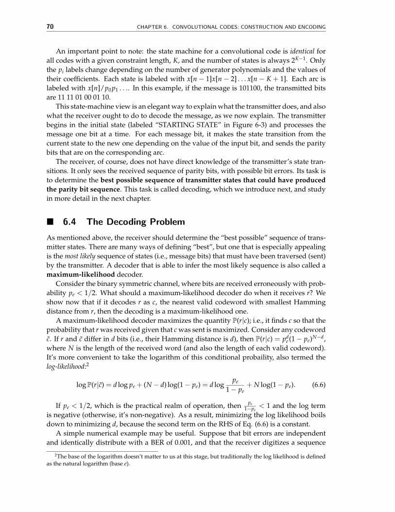
70 CHAPTER 6. CONVOLUTIONAL CODES: CONSTRUCTION AND ENCODING
An important point to note: the state machine for a convolutional code is identical forall codes with a given constraint length, K, and the number of states is always 2K−1. Onlythe pi labels change depending on the number of generator polynomials and the values oftheir coefficients. Each state is labeled with x[n− 1]x[n− 2] . . . x[n− K + 1]. Each arc islabeled with x[n]/p0 p1 . . .. In this example, if the message is 101100, the transmitted bitsare 11 11 01 00 01 10.
This state-machine view is an elegant way to explain what the transmitter does, and alsowhat the receiver ought to do to decode the message, as we now explain. The transmitterbegins in the initial state (labeled “STARTING STATE” in Figure 6-3) and processes themessage one bit at a time. For each message bit, it makes the state transition from thecurrent state to the new one depending on the value of the input bit, and sends the paritybits that are on the corresponding arc.
The receiver, of course, does not have direct knowledge of the transmitter’s state tran-sitions. It only sees the received sequence of parity bits, with possible bit errors. Its task isto determine the best possible sequence of transmitter states that could have producedthe parity bit sequence. This task is called decoding, which we introduce next, and studyin more detail in the next chapter.
� 6.4 The Decoding Problem
As mentioned above, the receiver should determine the “best possible” sequence of trans-mitter states. There are many ways of defining “best”, but one that is especially appealingis the most likely sequence of states (i.e., message bits) that must have been traversed (sent)by the transmitter. A decoder that is able to infer the most likely sequence is also called amaximum-likelihood decoder.
Consider the binary symmetric channel, where bits are received erroneously with prob-ability pe < 1/2. What should a maximum-likelihood decoder do when it receives r? Weshow now that if it decodes r as c, the nearest valid codeword with smallest Hammingdistance from r, then the decoding is a maximum-likelihood one.
A maximum-likelihood decoder maximizes the quantity P(r|c); i.e., it finds c so that theprobability that r was received given that c was sent is maximized. Consider any codewordc̃. If r and c̃ differ in d bits (i.e., their Hamming distance is d), then P(r|c) = pd
e (1− pe)N−d,where N is the length of the received word (and also the length of each valid codeword).It’s more convenient to take the logarithm of this conditional probaility, also termed thelog-likelihood:2
log P(r|c̃) = d log pe + (N− d) log(1− pe) = d logpe
1− pe+ N log(1− pe). (6.6)
If pe < 1/2, which is the practical realm of operation, then pe1−pe
< 1 and the log termis negative (otherwise, it’s non-negative). As a result, minimizing the log likelihood boilsdown to minimizing d, because the second term on the RHS of Eq. (6.6) is a constant.
A simple numerical example may be useful. Suppose that bit errors are independentand identically distribute with a BER of 0.001, and that the receiver digitizes a sequence
2The base of the logarithm doesn’t matter to us at this stage, but traditionally the log likelihood is definedas the natural logarithm (base e).

SECTION 6.4. THE DECODING PROBLEM 71
Msg Xmit* Rcvd d
0000 000000000000
111011000110
7
0001 000000111110 8
0010 000011111000 8
0011 000011010110 4
0100 001111100000 6
0101 001111011110 5
0110 001101001000 7
0111 001100100110 6
1000 111110000000 4
1001 111110111110 5
1010 111101111000 7
1011 111101000110 2
1100 110001100000 5
1101 110001011110 4
1110 110010011000 6
1111 110010100110 3
Most likely: 1011
Figure 6-4: When the probability of bit error is less than 1/2, maximum-likelihood decoding boils downto finding the message whose parity bit sequence, when transmitted, has the smallest Hamming distanceto the received sequence. Ties may be broken arbitrarily. Unfortunately, for an N-bit transmit sequence,there are 2N possibilities, which makes it hugely intractable to simply go through in sequence becauseof the sheer number. For instance, when N = 256 bits (a really small packet), the number of possibilitiesrivals the number of atoms in the universe!
of analog samples into the bits 1101001. Is the sender more likely to have sent 1100111or 1100001? The first has a Hamming distance of 3, and the probability of receiving thatsequence is (0.999)4(0.001)3 = 9.9× 10⁻¹⁰. The second choice has a Hamming distance of1 and a probability of (0.999)6(0.001)1 = 9.9× 10⁻⁴, which is six orders of magnitude higherand is overwhelmingly more likely.
Thus, the most likely sequence of parity bits that was transmitted must be the one withthe smallest Hamming distance from the sequence of parity bits received. Given a choiceof possible transmitted messages, the decoder should pick the one with the smallest suchHamming distance.
Determining the nearest valid codeword to a received word is easier said than done forconvolutional codes. For example, see Figure 6-4, which shows a convolutional code withK = 3 and rate 1/2. If the receiver gets 111011000110, then some errors have occurred,because no valid transmitted sequence matches the received one. The last column in theexample shows d, the Hamming distance to all the possible transmitted sequences, with

72 CHAPTER 6. CONVOLUTIONAL CODES: CONSTRUCTION AND ENCODING
Figure 6-5: The trellis is a convenient way of viewing the decoding task and understanding the time evo-lution of the state machine.
the smallest one circled. To determine the most-likely 4-bit message that led to the paritysequence received, the receiver could look for the message whose transmitted parity bitshave smallest Hamming distance from the received bits. (If there are ties for the smallest,we can break them arbitrarily, because all these possibilities have the same resulting post-coded BER.)
The straightforward approach of simply going through the list of possible transmit se-quences and comparing Hamming distances is horribly intractable. The reason is that atransmit sequence of N bits has 2N possible strings, a number that is simply too large foreven small values of N, like 256 bits. We need a better plan for the receiver to navigate thisunbelievable large space of possibilities and quickly determine the valid message withsmallest Hamming distance. We will study a powerful and widely applicable method forsolving this problem, called Viterbi decoding, in the next lecture. This decoding methoduses a special structure called the trellis, which we describe next.
� 6.5 The Trellis
The trellis is a structure derived from the state machine that will allow us to develop anefficient way to decode convolutional codes. The state machine view shows what happensat each instant when the sender has a message bit to process, but doesn’t show how thesystem evolves in time. The trellis is a structure that makes the time evolution explicit.An example is shown in Figure 6-5. Each column of the trellis has the set of states; eachstate in a column is connected to two states in the next column—the same two states inthe state diagram. The top link from each state in a column of the trellis shows what getstransmitted on a “0”, while the bottom shows what gets transmitted on a “1”. The picture

SECTION 6.5. THE TRELLIS 73
shows the links between states that are traversed in the trellis given the message 101100.We can now think about what the decoder needs to do in terms of this trellis. It gets a
sequence of parity bits, and needs to determine the best path through the trellis—that is,the sequence of states in the trellis that can explain the observed, and possibly corrupted,sequence of received parity bits.
The Viterbi decoder finds a maximum-likelihood path through the trellis. We willstudy it in the next chapter.
Problems and exercises on convolutional coding are at the end of the next chapter, after wediscuss the decoding process.

74 CHAPTER 6. CONVOLUTIONAL CODES: CONSTRUCTION AND ENCODING

MIT 6.02 DRAFT Lecture NotesLast update: October 9, 2011Comments, questions or bug reports?
Please contact hari at mit.edu
CHAPTER 7Viterbi Decoding of Convolutional
Codes
This chapter describes an elegant and efficient method to decode convolutional codes,whose construction and encoding we described in the previous chapter. This decodingmethod avoids explicitly enumerating the 2N possible combinations of N-bit parity bitsequences. This method was invented by Andrew Viterbi ’57 and bears his name.
� 7.1 The Problem
At the receiver, we have a sequence of voltage samples corresponding to the parity bits thatthe transmitter has sent. For simplicity, and without loss of generality, we will assume thatthe receiver picks a suitable sample for the bit, or better still, averages the set of samplescorresponding to a bit, digitizes that value to a “0” or “1” by comparing to the thresholdvoltage (the demapping step), and propagates that bit decision to the decoder.
Thus, we have a received bit sequence, which for a convolutionally coded stream cor-responds to the stream of parity bits. If we decode this received bit sequence with noother information from the receiver’s sampling and demapper, then the decoding processis termed hard decision decoding (“hard decoding”). If, in addition, the decoder is giventhe actual voltage samples and uses that information in decoding the data, we term theprocess soft decision decoding (“soft decoding”).
The Viterbi decoder can be used in either case. Intuitively, because hard decision de-coding makes an early decision regarding whether a bit is 0 or 1, it throws away infor-mation in the digitizing process. It might make a wrong decision, especially for voltagesnear the threshold, introducing a greater number of bit errors in the received bit sequence.Although it still produces the most likely transmitted sequence given the received bit se-quence, by introducing additional errors in the early digitization, the overall reduction inthe probability of bit error will be smaller than with soft decision decoding. But it is con-ceptually easier to understand hard decoding, so we will start with that, before going onto soft decoding.
As mentioned in the previous chapter, the trellis provides a good framework for un-
75

76 CHAPTER 7. VITERBI DECODING OF CONVOLUTIONAL CODES
Figure 7-1: The trellis is a convenient way of viewing the decoding task and understanding the time evo-lution of the state machine.
derstanding the decoding procedure for convolutional codes (Figure 7-1). Suppose wehave the entire trellis in front of us for a code, and now receive a sequence of digitizedbits (or voltage samples). If there are no errors (i.e., the signal-to-noise ratio, SNR, is highenough), then there will be some path through the states of the trellis that would exactlymatch the received sequence. That path (specifically, the concatenation of the encoding ofeach state along the path) corresponds to the transmitted parity bits. From there, gettingto the original message is easy because the top arc emanating from each node in the trelliscorresponds to a “0” bit and the bottom arrow corresponds to a “1” bit.
When there are bit errors, what can we do? As explained earlier, finding the most likelytransmitted message sequence is appealing because it minimizes the BER. If we can comeup with a way to capture the errors introduced by going from one state to the next, thenwe can accumulate those errors along a path and come up with an estimate of the totalnumber of errors along the path. Then, the path with the smallest such accumulation oferrors is the path we want, and the transmitted message sequence can be easily determinedby the concatenation of states explained above.
To solve this problem, we need a way to capture any errors that occur in going throughthe states of the trellis, and a way to navigate the trellis without actually materializing theentire trellis (i.e., without enumerating all possible paths through it and then finding theone with smallest accumulated error). The Viterbi decoder solves these problems. It isan example of a more general approach to solving optimization problems, called dynamicprogramming. Later in the course, we will apply similar concepts in network routing, anunrelated problem, to find good paths in multi-hop networks.

SECTION 7.2. THE VITERBI DECODER 77
Figure 7-2: The branch metric for hard decision decoding. In this example, the receiver gets the parity bits00.
� 7.2 The Viterbi Decoder
The decoding algorithm uses two metrics: the branch metric (BM) and the path metric(PM). The branch metric is a measure of the “distance” between what was transmitted andwhat was received, and is defined for each arc in the trellis. In hard decision decoding,where we are given a sequence of digitized parity bits, the branch metric is the Hammingdistance between the expected parity bits and the received ones. An example is shown inFigure 7-2, where the received bits are 00. For each state transition, the number on the arcshows the branch metric for that transition. Two of the branch metrics are 0, correspondingto the only states and transitions where the corresponding Hamming distance is 0. Theother non-zero branch metrics correspond to cases when there are bit errors.
The path metric is a value associated with a state in the trellis (i.e., a value associatedwith each node). For hard decision decoding, it corresponds to the Hamming distanceover the most likely path from the initial state to the current state in the trellis. By “mostlikely”, we mean the path with smallest Hamming distance between the initial state andthe current state, measured over all possible paths between the two states. The path withthe smallest Hamming distance minimizes the total number of bit errors, and is most likelywhen the BER is low.
The key insight in the Viterbi algorithm is that the receiver can compute the path metricfor a (state, time) pair incrementally using the path metrics of previously computed statesand the branch metrics.
� 7.2.1 Computing the Path Metric
Suppose the receiver has computed the path metric PM[s, i] for each state s at time stepi (recall that there are 2K−1 states, where K is the constraint length of the convolutionalcode). In hard decision decoding, the value of PM[s, i] is the total number of bit errorsdetected when comparing the received parity bits to the most likely transmitted message,considering all messages that could have been sent by the transmitter until time step i(starting from state “00”, which we will take to be the starting state always, by convention).

78 CHAPTER 7. VITERBI DECODING OF CONVOLUTIONAL CODES
Among all the possible states at time step i, the most likely state is the one with thesmallest path metric. If there is more than one such state, they are all equally good possi-bilities.
Now, how do we determine the path metric at time step i + 1, PM[s, i + 1], for each states? To answer this question, first observe that if the transmitter is at state s at time step i + 1,then it must have been in only one of two possible states at time step i. These two predecessorstates, labeled α and β, are always the same for a given state. In fact, they depend onlyon the constraint length of the code and not on the parity functions. Figure 7-2 shows thepredecessor states for each state (the other end of each arrow). For instance, for state 00,α = 00 and β = 01; for state 01, α = 10 and β = 11.
Any message sequence that leaves the transmitter in state s at time i + 1 must have leftthe transmitter in state α or state β at time i. For example, in Figure 7-2, to arrive in state’01’ at time i + 1, one of the following two properties must hold:
1. The transmitter was in state ‘10’ at time i and the ith message bit was a 0. If that isthe case, then the transmitter sent ‘11’ as the parity bits and there were two bit errors,because we received the bits 00. Then, the path metric of the new state, PM[‘01’, i + 1]is equal to PM[‘10’, i] + 2, because the new state is ‘01’ and the corresponding pathmetric is larger by 2 because there are 2 errors.
2. The other (mutually exclusive) possibility is that the transmitter was in state ‘11’ attime i and the ith message bit was a 0. If that is the case, then the transmitter sent 01as the parity bits and tere was one bit error, because we received 00. The path metricof the new state, PM[‘01’, i + 1] is equal to PM[‘11’, i] + 1.
Formalizing the above intuition, we can see that
PM[s, i + 1] = min(PM[α, i] + BM[α→ s],PM[β, i] + BM[β→ s]), (7.1)
where α and β are the two predecessor states.In the decoding algorithm, it is important to remember which arc corresponds to the
minimum, because we need to traverse this path from the final state to the initial onekeeping track of the arcs we used, and then finally reverse the order of the bits to producethe most likely message.
� 7.2.2 Finding the Most Likely Path
We can now describe how the decoder finds the maximum-likelihood path. Initially, state‘00’ has a cost of 0 and the other 2k−1− 1 states have a cost of∞.
The main loop of the algorithm consists of two main steps: first, calculating the branchmetric for the next set of parity bits, and second, computing the path metric for the nextcolumn. The path metric computation may be thought of as an add-compare-select proce-dure:
1. Add the branch metric to the path metric for the old state.2. Compare the sums for paths arriving at the new state (there are only two such paths
to compare at each new state because there are only two incoming arcs from theprevious column).
3. Select the path with the smallest value, breaking ties arbitrarily. This path corre-sponds to the one with fewest errors.

SECTION 7.3. SOFT DECISION DECODING 79
Figure 7-3 shows the decoding algorithm in action from one time step to the next. Thisexample shows a received bit sequence of 11 10 11 00 01 10 and how the receiver processesit. The fourth picture from the top shows all four states with the same path metric. At thisstage, any of these four states and the paths leading up to them are most likely transmittedbit sequences (they all have a Hamming distance of 2). The bottom-most picture showsthe same situation with only the survivor paths shown. A survivor path is one that hasa chance of being the maximum-likelihood path; there are many other paths that can bepruned away because there is no way in which they can be most likely. The reason whythe Viterbi decoder is practical is that the number of survivor paths is much, much smallerthan the total number of paths in the trellis.
Another important point about the Viterbi decoder is that future knowledge will help itbreak any ties, and in fact may even cause paths that were considered “most likely” at acertain time step to change. Figure 7-4 continues the example in Figure 7-3, proceeding un-til all the received parity bits are decoded to produce the most likely transmitted message,which has two bit errors.
� 7.3 Soft Decision Decoding
Hard decision decoding digitizes the received voltage signals by comparing it to a thresh-old, before passing it to the decoder. As a result, we lose information: if the voltage was0.500001, the confidence in the digitization is surely much lower than if the voltage was0.999999. Both are treated as “1”, and the decoder now treats them the same way, eventhough it is overwhelmingly more likely that 0.999999 is a “1” compared to the other value.
Soft decision decoding (also sometimes known as “soft input Viterbi decoding”) buildson this observation. It does not digitize the incoming samples prior to decoding. Rather, it usesa continuous function of the analog sample as the input to the decoder. For example, if theexpected parity bit is 0 and the received voltage is 0.3 V, we might use 0.3 (or 0.32, or somesuch function) as the value of the “bit” instead of digitizing it.
For technical reasons that will become apparent later, an attractive soft decision metricis the square of the difference between the received voltage and the expected one. If theconvolutional code produces p parity bits, and the p corresponding analog samples arev = v1, v2, . . . , vp, one can construct a soft decision branch metric as follows
BMsoft[u, v] =p
∑i=1
(ui − vi)2, (7.2)
where u = u1, u2, . . . , up are the expected p parity bits (each a 0 or 1). Figure 7-5 shows thesoft decision branch metric for p = 2 when u is 00.
With soft decision decoding, the decoding algorithm is identical to the one previouslydescribed for hard decision decoding, except that the branch metric is no longer an integerHamming distance but a positive real number (if the voltages are all between 0 and 1, thenthe branch metric is between 0 and 1 as well).
It turns out that this soft decision metric is closely related to the probability of the decodingbeing correct when the channel experiences additive Gaussian noise. First, let’s look at thesimple case of 1 parity bit (the more general case is a straightforward extension). Suppose

80 CHAPTER 7. VITERBI DECODING OF CONVOLUTIONAL CODES
the receiver gets the ith parity bit as vi volts. (In hard decision decoding, it would decode− as 0 or 1 depending on whether vi was smaller or larger than 0.5.) What is the probabilitythat vi would have been received given that bit ui (either 0 or 1) was sent? With zero-meanadditive Gaussian noise, the PDF of this event is given by
f (vi|ui) =e−d2
i /2σ2
√2πσ2
, (7.3)
where di = v2i if ui = 0 and di = (vi − 1)2 if ui = 1.
The log likelihood of this PDF is proportional to −d2i . Moreover, along a path, the PDF
of the sequence V = v1, v2, . . . , vp being received given that a code word U = ui, u2, . . . , up
was sent, is given by the product of a number of terms each resembling Eq. (7.3). Thelogarithm of this PDF for the path is equal to the sum of the individual log likelihoods,and is proportional to −∑i d2
i . But that’s precisely the negative of the branch metric wedefined in Eq. (7.2), which the Viterbi decoder minimizes along the different possiblepaths! Minimizing this path metric is identical to maximizing the log likelihood alongthe different paths, implying that the soft decision decoder produces the most likely paththat is consistent with the received voltage sequence.
This direct relationship with the logarithm of the probability is the reason why we chosethe sum of squares as the branch metric in Eq. (7.2). A different noise distribution (otherthan Gaussian) may entail a different soft decoding branch metric to obtain an analogousconnection to the PDF of a correct decoding.
� 7.4 Achieving Higher and Finer-Grained Rates: Puncturing
As described thus far, a convolutional code achieves a maximum rate of 1/r, where r is thenumber of parity bit streams produced by the code. But what if we want a rate greaterthan 1/2, or a rate between 1/r and 1/(r + 1) for some r?
A general technique called puncturing gives us a way to do that. The idea is straight-forward: the encoder does not send every parity bit produced on each stream, but “punc-tures” the stream sending only a subset of the bits that are agreed-upon between the en-coder and decoder. For example, one might use a rate-1/2 code along with the puncturingschedule specified as a vector; for example, we might use the vector (101) on the first paritystream and (110) on the second. This notation means that the encoder sends the first andthird bits but not the second bit on the first stream, and sends the first and second bits butnot the third bit on the second stream. Thus, whereas the encoder would have sent twoparity bits for every message bit without puncturing, it would now send four parity bits(instead of six) for every three message bits, giving a rate of 3/4.
In this example, suppose the sender in the rate-1/2 code, without puncturing, emittedbits p0[0]p1[0]p0[1]p1[1]p0[2]p1[2] . . .. Then, with the puncturing schedule given, the bitsemitted would be p0[0]p1[0]− p1[1]p0[2]− . . ., where each − refers to an omitted bit.
At the decoder, when using a punctured code, missing parity bits don’t participate inthe calculation of branch metrics. Otherwise, the procedure is the same as before. We canthink of each missing parity bit as a blank (’−’) and run the decoder by just skipping overthe blanks.

SECTION 7.5. PERFORMANCE ISSUES 81
� 7.5 Performance Issues
There are three important performance metrics for convolutional coding and decoding:
1. How much state and space does the encoder need?
2. How much time does the decoder take?
3. What is the reduction in the bit error rate, and how does that compare with othercodes?
� 7.5.1 Encoder and Decoder Complexity
The first question is the easiest: the amount of space is linear in K, the constraint length,and the encoder is much easier to implement than the Viterbi decoder. The decoding timedepends mainly on K; as described, we need to process O(2K) transitions each bit time, sothe time complexity is exponential in K. Moreover, as described, we can decode the firstbits of the message only at the very end. A little thought will show that although a little fu-ture knowledge is useful, it is unlikely that what happens at bit time 1000 will change ourdecoding decision for bit 1, if the constraint length is, say, 6. In fact, in practice the decoderstarts to decode bits once it has reached a time step that is a small multiple of the constraintlength; experimental data suggests that 5 · K message bit times (or thereabouts) is a rea-sonable decoding window, regardless of how long the parity bit stream corresponding tothe message it.
� 7.5.2 Free Distance
The reduction in error probability and comparisons with other codes is a more involvedand detailed issue. The answer depends on the constraint length (generally speaking,larger K has better error correction), the number of generators (larger this number, thelower the rate, and the better the error correction), and the amount of noise.
In fact, these factors are indirect proxies for the free distance, which largely determineshow well a convolutional code corrects errors. Because convolutional codes are linear, ev-erything we learned about linear codes applies here. In particular, the Hamming distanceof a linear code, i.e., the minimum Hamming distance between any two valid codewords,is equal to the number of ones in the smallest non-zero codeword with minimum weight,where the weight of a codeword is the number of ones it contains.
In the context of convolutional codes, the smallest Hamming distance between any twovalid codewords is called the free distance. Specifically, the free distance of a convolutionalcode is the difference in path metrics between the all-zeroes output and the path withthe smallest non-zero path metric going from the initial 00 state to some future 00 state.Figure 7-6 illustrates this notion with an example. In this example, the free distance is 4,and it takes 8 output bits to get back to the correct state, so one would expect this codeto be able to correct up to b(4− 1)/2c = 1 bit error in blocks of 8 bits, if the block starts atthe first parity bit. In fact, this error correction power is essentially the same as an (8,4,3)rectangular parity code. Note that the free distance in this example is 4, not 5: the smallestnon-zero path metric between the initial 00 state and a future 00 state goes like this: 00→10→ 11→ 01→ 00 and the corresponding path metrics increase as 0→ 2→ 2→ 3→ 4.

82 CHAPTER 7. VITERBI DECODING OF CONVOLUTIONAL CODES
Why do we define a “free distance”, rather than just call it the Hamming distance, if itis defined the same way? The reason is that any code with Hamming distance D (whetherlinear or not) can correct all patterns of up to bD−1
2 c errors. If we just applied the samenotion to convolutional codes, we will conclude that we can correct all single-bit errors inthe example given, or in general, we can correct some fixed number of errors.
Now, convolutional coding produces an unbounded bit stream; these codes aremarkedly distinct from block codes in this regard. As a result, the bD−1
2 c formula is nottoo instructive because it doesn’t capture the true error correction properties of the code.A convolutional code (with Viterbi decoding) can correct t = bD−1
2 c errors as long as theseerrors are “far enough apart”. So the notion we use is the free distance because, in a sense,errors can keep occurring and as long as no more than t of them occur in a closely spacedburst, the decoder can correct them all.
� 7.5.3 Comparing Codes: Simulation Results
In addition to the performance different hard decision convolutional codes, an importantquestion is how much better soft decision decoding is compared to hard decision decoding.We address these questions by describing some simulation results here.
Figure 7-7 shows some representative performance results for a set of codes all of thesame code rate (1/2).1 The top-most curve shows the uncoded probability of bit error,which may be modeled using the erfc function. The x axis plots the SNR on the dB scale,as defined in Chapter 5 (lower noise is toward the right). The y axis shows the probabilityof a decoding error on a log scale.
This figure shows the performance of three codes:
1. The (8,4,3) rectangular parity code.
2. A convolutional code with generators (111,100) and constraint length K = 3, shownin the picture as “K = 3”.
3. A convolutional code with generators (1110,1101) and constraint length K = 4,shown in the picture as “K = 4”.
Some observations:
1. The probability of error is roughly the same for the rectangular parity code and harddecision decoding with K = 3. The free distance of the K = 3 convolutional code is 4,which means it can correct one bit error over blocks that are similar in length to therectangular parity code we are comparing with. Intuitively, both schemes essentiallyproduce parity bits that are built from similar amounts of history. In the rectangularparity case, the row parity bit comes from two successive message bits, while thecolumn parity comes from two message bits with one skipped in between. But wealso send the message bits, so we’re mimicking a similar constraint length (amountof memory) to the K = 3 convolutional code.
1You will produce similar pictures in one of your lab tasks using your implementations of the Viterbi andrectangular parity code decoders.
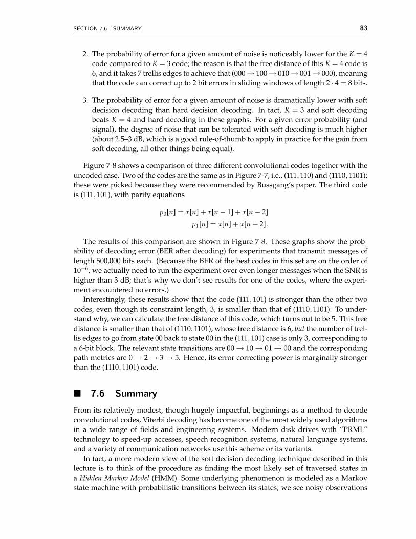
SECTION 7.6. SUMMARY 83
2. The probability of error for a given amount of noise is noticeably lower for the K = 4code compared to K = 3 code; the reason is that the free distance of this K = 4 code is6, and it takes 7 trellis edges to achieve that (000→ 100→ 010→ 001→ 000), meaningthat the code can correct up to 2 bit errors in sliding windows of length 2 · 4 = 8 bits.
3. The probability of error for a given amount of noise is dramatically lower with softdecision decoding than hard decision decoding. In fact, K = 3 and soft decodingbeats K = 4 and hard decoding in these graphs. For a given error probability (andsignal), the degree of noise that can be tolerated with soft decoding is much higher(about 2.5–3 dB, which is a good rule-of-thumb to apply in practice for the gain fromsoft decoding, all other things being equal).
Figure 7-8 shows a comparison of three different convolutional codes together with theuncoded case. Two of the codes are the same as in Figure 7-7, i.e., (111,110) and (1110,1101);these were picked because they were recommended by Bussgang’s paper. The third codeis (111,101), with parity equations
p0[n] = x[n] + x[n− 1] + x[n− 2]
p1[n] = x[n] + x[n− 2].
The results of this comparison are shown in Figure 7-8. These graphs show the prob-ability of decoding error (BER after decoding) for experiments that transmit messages oflength 500,000 bits each. (Because the BER of the best codes in this set are on the order of10−6, we actually need to run the experiment over even longer messages when the SNR ishigher than 3 dB; that’s why we don’t see results for one of the codes, where the experi-ment encountered no errors.)
Interestingly, these results show that the code (111,101) is stronger than the other twocodes, even though its constraint length, 3, is smaller than that of (1110,1101). To under-stand why, we can calculate the free distance of this code, which turns out to be 5. This freedistance is smaller than that of (1110,1101), whose free distance is 6, but the number of trel-lis edges to go from state 00 back to state 00 in the (111,101) case is only 3, corresponding toa 6-bit block. The relevant state transitions are 00→ 10→ 01→ 00 and the correspondingpath metrics are 0→ 2→ 3→ 5. Hence, its error correcting power is marginally strongerthan the (1110,1101) code.
� 7.6 Summary
From its relatively modest, though hugely impactful, beginnings as a method to decodeconvolutional codes, Viterbi decoding has become one of the most widely used algorithmsin a wide range of fields and engineering systems. Modern disk drives with “PRML”technology to speed-up accesses, speech recognition systems, natural language systems,and a variety of communication networks use this scheme or its variants.
In fact, a more modern view of the soft decision decoding technique described in thislecture is to think of the procedure as finding the most likely set of traversed states ina Hidden Markov Model (HMM). Some underlying phenomenon is modeled as a Markovstate machine with probabilistic transitions between its states; we see noisy observations

84 CHAPTER 7. VITERBI DECODING OF CONVOLUTIONAL CODES
from each state, and would like to piece together the observations to determine the mostlikely sequence of states traversed. It turns out that the Viterbi decoder is an excellentstarting point to solve this class of problems (and sometimes the complete solution).
On the other hand, despite its undeniable success, Viterbi decoding isn’t the only wayto decode convolutional codes. For one thing, its computational complexity is exponentialin the constraint length, K, because it does require each of these states to be enumerated.When K is large, one may use other decoding methods such as BCJR or Fano’s sequentialdecoding scheme, for instance.
Convolutional codes themselves are very popular over both wired and wireless links.They are sometimes used as the “inner code” with an outer block error correcting code,but they may also be used with just an outer error detection code. They are also usedas a component in more powerful codes line turbo codes, which are currently one of thehighest-performing codes used in practice.
� Problems and Exercises
1. Please check out and solve the online problems on error correction codes athttp://web.mit.edu/6.02/www/f2011/handouts/tutprobs/ecc.html
2. Consider a convolutional code whose parity equations are
p0[n] = x[n] + x[n− 1] + x[n− 3]
p1[n] = x[n] + x[n− 1] + x[n− 2]
p2[n] = x[n] + x[n− 2] + x[n− 3]
(a) What is the rate of this code? How many states are in the state machine repre-sentation of this code?
(b) Suppose the decoder reaches the state “110” during the forward pass of theViterbi algorithm with this convolutional code.
i. How many predecessor states (i.e., immediately preceding states) does state“110” have?
ii. What are the bit-sequence representations of the predecessor states of state“110”?
iii. What are the expected parity bits for the transitions from each of these pre-decessor states to state “110”? Specify each predecessor state and the ex-pected parity bits associated with the corresponding transition below.
(c) To increase the rate of the given code, Lem E. Tweakit punctures the p0 paritystream using the vector (1 0 1 1 0), which means that every second and fifth bitproduced on the stream are not sent. In addition, she punctures the p1 paritystream using the vector (1 1 0 1 1). She sends the p2 parity stream unchanged.What is the rate of the punctured code?
3. Let conv encode(x) be the resulting bit-stream after encoding bit-string x with aconvolutional code, C. Similarly, let conv decode(y) be the result of decoding yto produce the maximum-likelihood estimate of the encoded message. Suppose we

SECTION 7.6. SUMMARY 85
send a message M using code C over some channel. Let P = conv encode(M) andlet R be the result of sending P over the channel and digitizing the received samplesat the receiver (i.e., R is another bit-stream). Suppose we use Viterbi decoding onR, knowing C, and find that the maximum-likelihood estimate of M is M̂. Duringthe decoding, we find that the minimum path metric among all the states in the finalstage of the trellis is Dmin.
Dmin is the Hamming distance between and . Fill in theblanks, explaining your answer.

86 CHAPTER 7. VITERBI DECODING OF CONVOLUTIONAL CODES
Figure 7-3: The Viterbi decoder in action. This picture shows four time steps. The bottom-most picture isthe same as the one just before it, but with only the survivor paths shown.

SECTION 7.6. SUMMARY 87
Figure 7-4: The Viterbi decoder in action (continued from Figure 7-3. The decoded message is shown. Toproduce this message, start from the final state with smallest path metric and work backwards, and thenreverse the bits. At each state during the forward pass, it is important to remeber the arc that got us to thisstate, so that the backward pass can be done properly.

88 CHAPTER 7. VITERBI DECODING OF CONVOLUTIONAL CODES
0.0,1.0 1.0,1.0
Vp0,Vp1
So# metric when expected parity bits are 0,0
0.0,0.0 1.0,0.0
V2p0 + V2
p1
Figure 7-5: Branch metric for soft decision decoding.
00
01
10
11
0/00 1/11
0/10
1/01
1/00 0/11
0/01 1/10
time
x[n-1]x[n-2]
x[n] 0 0 0 0 0 0
0/00 1/11
0/10
1/01
1/00 0/11
0/01 1/10
0/00 1/11
0/10
1/01
1/00 0/11
0/01 1/10
0/00 1/11
0/10
1/01
1/00 0/11
0/01 1/10
0/00 1/11
0/10
1/01
1/00 0/11
0/01 1/10
0/00 1/11
0/10
1/01
1/00 0/11
0/01 1/10
2
00 00 00
The free distance is the difference in path metrics between the all-zeroes output and the path with the smallest non-zero path metric going from the initial 00 state to some future 00 state. It is 4 in this example. The path 00 à 10 à01 à 00 has
a shorter length, but a higher path metric (of 5), so it is not the free distance.
2
3
4 00
Figure 7-6: The free distance of a convolutional code.

SECTION 7.6. SUMMARY 89
Figure 7-7: Error correcting performance results for different rate-1/2 codes.
Figure 7-8: Error correcting performance results for three different rate-1/2 convolutional codes. The pa-rameters of the three convolutional codes are (111,110) (labeled “K = 3 glist=(7,6)”), (1110,1101) (labeled“K = 4 glist=(14,13)”), and (111,101) (labeled “K = 3 glist=(7,5)”). The top three curves below the uncodedcurve are for hard decision decoding; the bottom three curves are for soft decision decoding.