BIS Working Papers No 399

Global safe assets

by Pierre-Olivier Gourinchas and Olivier Jeanne

Monetary and Economic Department

December 2012

JEL classification: safe assets, dollar, euro, liquidity trap, government debt crisis Keywords: F02, F30, G01, G15

BIS Working Papers are written by members of the Monetary and Economic Department of the Bank for International Settlements, and from time to time by other economists, and are published by the Bank. The papers are on subjects of topical interest and are technical in character. The views expressed in them are those of their authors and not necessarily the views of the BIS.

This publication is available on the BIS website (www.bis.org).

© Bank for International Settlements 2012. All rights reserved. Brief excerpts may be reproduced or translated provided the source is stated.

ISSN 1020-0959 (print)

ISSN 1682-7678(online)

iii

Foreword

On 21–22 June 2012, the BIS held its Eleventh Annual Conference, on “The future of financial globalisation” in Lucerne, Switzerland. The event brought together senior representatives of central banks and academic institutions who exchanged views on this topic. The papers presented at the conference and the discussants’ comments are released as BIS Working Papers 397 to 400. A forthcoming BIS Paper will contain the opening address Stephen Cecchetti (Economic Adviser, BIS), a keynote address from Amartya Sen (Harvard University), and the available contributions of the policy panel on “Will financial globalisation survive?”. The participants in the policy panel discussion, chaired by Jaime Caruana (General Manager, BIS), were Ravi Menon (Monetary Authority of Singapore), Jacob Frenkel (JP Morgan Chase International) and José Dario Uribe Escobar (Banco de la Repubblica).

iv

Contents

Foreword ............................................................................................................................... iii Programme ............................................................................................................................ v

Global Safe Assets by Pierre-Olivier Gourinchas and Olivier Jeanne ........................................................... 1

Discussant comments by Peter R Fisher ........................................................................ 53 Discussant comments by Fabrizio Saccomanni .............................................................. 56

v

Programme

Thursday 21 June 2012

12:15-13:30 Informal buffet luncheon

13:45-14:00 Opening remarks by Stephen Cecchetti (BIS)

14:00-15:30 Session 1: Revisiting the costs and benefits of financial globalisation

Chair: Gill Marcus (Governor, South African Reserve Bank)

Author: Philip Lane (Trinity College Dublin) "Financial Globalisation and the Crisis"

Discussant: Dani Rodrik (Harvard Kennedy School) Coffee break (30 min) 16:00-17:30 Session 2: Financial globalisation and the Great Leveraging

Chair: Alexandre Tombini (Governor, Banco Central do Brasil)

Author: Alan Taylor (University of Virginia)

"The Great Leveraging"

Discussants: Barry Eichengreen (University of California, Berkeley) Y Venugopal Reddy (Former Governor, Reserve Bank of India - University of Hyderabad)

18.00 Departure from the Palace hotel for dinner venue (Mount Pilatus)

19:30 Dinner Keynote lecture: Amartya Sen (Harvard University) Friday 22 June 2012

09:00-10.30 Session 3: Financial globalisation in a world without a riskless asset Chair: Erdem Basçi (Governor, Central Bank of Turkey)

Author: Pierre Olivier Gourinchas (University of California, Berkeley) and Olivier Jeanne (Johns Hopkins University) “Global Safe Assets”

Discussants: Peter Fisher (BlackRock) Fabrizio Saccomanni (Director General, Banca d’Italia) Coffee break (30 min)

vi

11:00-12.30 Session 4: Financial globalisation and monetary policy Chair: Masaaki Shirakawa (Governor, Bank of Japan)

Author: Hyun Song Shin (Princeton University) “Capital Flows and the Risk-Taking Channel of Monetary Policy”

Discussants: John Taylor (Stanford University) Lars Svensson (Deputy Governor, Sveriges Riksbank)

12.30 Lunch Speaker: Jean-Claude Trichet (former ECB President, Chair G30)

14:00-15:30 Panel discussion “Will financial globalisation survive?” Chair: Jaime Caruana (BIS)

Panellists: Ravi Menon (Managing Director, Monetary Authority of Singapore) Jacob Frenkel (Chairman, JP Morgan Chase International) José Dario Uribe Escobar (Governor, Banco de la República)

Global Safe Assets∗

Pierre-Olivier Gourinchas§

University of California at Berkeley

Olivier Jeanne∗∗

Johns Hopkins University

Abstract

Will the world run out of ‘safe assets’ and what would be the consequences on globalfinancial stability? We argue that in a world with competing private stores of value, theglobal economic system tends to favor the riskiest ones. Privately produced stores ofvalue cannot provide sufficient insurance against global shocks. Only public safe assetsmay, if appropriately supported by monetary policy. We draw some implications forthe global financial system.

∗This paper was prepared for the XI BIS Annual Conference held in Lucerne, June 20-21 2012. We wish tothank conference participants and especially Peter Fisher and Fabrizio Saccomanni for excellent comments.Victoria Vanasco and Gee Hee Hong provided excellent research assistance.§Also affiliated with the National Bureau of Economic Research (Cambridge), and the Center for Economic

Policy Research (London). Contact address: UC Berkeley, Department of Economics, 691A Evans Hall#3880, Berkeley, CA 94720-3880. email: pog@berkeley.edu. This draft was completed while the author wasvisiting the Paris School of Economics, whose hospitality is gratefully acknowledged. Financial assistancefrom the International Growth Center (grant RA-2009-11-002) is gratefully acknowledged.∗∗Also affiliated with the Peterson Institute for International Economics (Washington DC), the National

Bureau of Economic Research (Cambridge), and the Center for Economic Policy Research (London). Contactaddress: Department of Economics, Johns Hopkins University, Mergenthaler Hall 454, 3400 N. Charles Street,Baltimore MD 21218. Email: ojeanne@jhu.edu.

1 Introduction

The notion that the global economy could be faced with a shortage of safe assets has become

a significant theme in recent policy debates (see inter alia Caballero, 2010b, Garcia, 2011,

Credit Suisse, 2011, and especially International Monetary Fund, 2012, chap. 3). Safe assets

are a cornerstone of modern financial systems. They provide a reliable store of value, serve

as collateral in financial transactions, fulfill prudential requirements, and serve as a pricing

benchmark. Should they disappear, the argument goes, the danger is that the financial

system itself might crumble. Markets for collateralized transactions (repos) would collapse;

financial institutions would have difficulties meeting their prudential requirements, and the

pricing and well-functioning of riskier segments of the financial system could be derailed

altogether. More daunting perhaps, households, retirees and firms would live in a world

without a suitably safe store of value. Without this safe anchor, the financial system would

experience greater systemic instability. As recently as April 2012, the IMF in chapter 3 of

its Global Financial Stability Report (2012, p.1), expressed the concern that “the shrinking

set of assets perceived as safe, now limited to mostly high-quality sovereign debt, coupled

with growing demand, can have negative implications for global financial stability.”

Indeed, a convincing link can be established between macroeconomic shortages of safe

assets and some of the most disturbing features of our recent global financial history. For

instance, Caballero, Farhi and Gourinchas (2008) or Bernanke (2005) discuss how the rapid

economic growth of emerging economies, coupled with a relative backwardness in financial

development created a global shortage of stores of value. This shortage depressed world

interest rates and fueled ‘global imbalances.’ This growing external demand for safe stores

of value also proved a powerful stimulant for US and European financial markets. Between

2002 and 2007, they manufactured large amounts of ‘private label’ safe assets through the

securitization of riskier assets (see Bernanke, Bertaut, DeMarco and Kamin, 2011).

The global financial crisis arose when many of these ‘private label’ safe assets –perceived

1

as safe because they were bestowed with a AAA rating– lost that quality. The sudden

realization that many of the safe assets undergirding the entire financial system were of

questionable value led to a ‘sudden financial arrest’ (Caballero, 2010a). In the subsequent

unraveling, most of these ‘private label’ safe assets disappeared. In the euro area, the strains

associated with the crisis quickly morphed into concerns about the safety of sovereign debts,

as governments simultaneously tried to shore up their financial sector and to sustain domestic

economic activity. This led to further shrinkage in the global supply of safe assets at the

same time that deleveraging financial institutions, panicked investors and anxious reserve

managers all tried to fly to safety.

In short, macroeconomic shortages of safe assets can create financial instability. Crises,

when they occur, further exacerbate the shortage that gave rise to it. Policy responses

designed to cope with the crisis such as liquidity injections and monetary easing prolong

the conditions for financial instability and delay the necessary balance sheet adjustment of

households and financial institutions (see BIS, 2011).

Could this destabilizing positive feedback loop lead to the ultimate disappearance of safe

assets –a recognition that nothing is really safe– with potentially disastrous consequences

for financial stability?

We argue in this paper that this analysis is incomplete. In particular, it ignores that the

global economy also exhibits poweful stabilizing mechanisms. One such mechanism, at work

both before and during the crisis, is the decline in the natural real interest rate, resulting

from the excess demand for stores of value. Figure 1 plots three different measures of global

real interest rates: a world short term real rate, defined as the GDP weighted average of G7 3-

months nominal interest rates minus ex-post inflation, a U.S. 10 year real rate defined as the

annualized yield on 10-year government bonds minus annualized 10-year expected inflation

from the Survey of Professional Forecasters, and the 10-year annualized yield on Inflation-

indexed Treasuries. All three measures illustrate the strong decline in global real interest

2

rates. In the case of the short term real rate, it reached -2.7 percent (p.a.) towards the end

of 2011. The decline in the natural rate operates both on the intensive and the extensive

margins. At the intensive margin, it increases the market value of existing assets, hence their

supply. Simultaneously, it improves the solvency of borrowers, especially sovereign ones. In

addition, the mechanism operates also at the extensive margin, stimulating the supply of

additional stores of value, i.e. stimulating borrowing. The important economic insight is that

while this additional borrowing can further fragilize the economy, as emphasized in Diamond

and Rajan (2011) and BIS (2011), it also contributes to an increase in stores of value, i.e. a

self-correcting mechanism. It is the tension between the fragility induced by the additional

leverage, and the stabilization induced by the additional supply of stores of value that is of

interest to us. In particular, we are interested in understanding the way in which monetary

policy can potentially contribute to the strengthening of the financial system. As we will

see, monetary policy will be important along two margins. First, it will need to accompany

the decline in the natural rate that occurs when the scarcity of stores of value becomes more

acute. Second, monetary policy can also play an important role as a backstop for public

securities. We show that a natural way to eliminate the financial instability arising from

the asset scarcity consists in supplying public safe assets. In turn, the safety of public asset

may require a monetary backstop. We show that this backstop can increase significantly the

safety of public securities, with minimal or no consequences in terms of price stability.

This mechanism is illustrated in its purest form in the Samuelsonian’s emergence of pure

rational bubbles (e.g. fiat money) in economies that suffer from a shortage of stores of values

(Samuelson, 1958). As we show with a model,1 if these bubbles were ‘safe’, in the sense of

1This model makes a number of simplifying assumptions. For instance, the financial bubbles that we willconsider here are of the ‘rational’ kind. A good argument can be made that departures from fundamentalvaluation may not simply reflect rational behavior, but also cognitive biases, institutional constraints, andlimits to arbitrage. That we do not consider these here does not mean these things are not important,simply that we can convey our point in a simple manner without making reference to them. Similarly, ourmodel does not feature financial frictions –beyond the fundamental market incompleteness that gives riseto a demand for stores of value. Financial frictions and/or agency problems are critical to many policyquestions and this simplification is also meant to keep our analysis as simple as possible, not to claim these

3

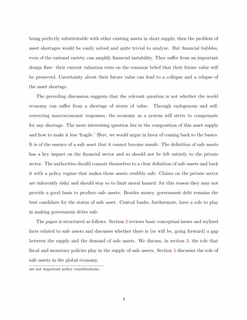
being perfectly substitutable with other existing assets in short supply, then the problem of

asset shortages would be easily solved and quite trivial to analyze. But financial bubbles,

even of the rational variety, can amplify financial instability. They suffer from an important

design flaw: their current valuation rests on the common belief that their future value will

be preserved. Uncertainty about their future value can lead to a collapse and a relapse of

the asset shortage.

The preceding discussion suggests that the relevant question is not whether the world

economy can suffer from a shortage of stores of value. Through endogenous and self-

correcting macroeconomic responses, the economy as a system will strive to compensate

for any shortage. The more interesting question lies in the composition of this asset supply

and how to make it less ‘fragile.’ Here, we would argue in favor of coming back to the basics.

It is of the essence of a safe asset that it cannot become unsafe. The definition of safe assets

has a key impact on the financial sector and so should not be left entirely to the private

sector. The authorities should commit themselves to a clear definition of safe assets and back

it with a policy regime that makes those assets credibly safe. Claims on the private sector

are inherently risky and should stay so to limit moral hazard: for this reason they may not

provide a good basis to produce safe assets. Besides money, government debt remains the

best candidate for the status of safe asset. Central banks, furthermore, have a role to play

in making government debts safe.

The paper is structured as follows. Section 2 reviews basic conceptual issues and stylized

facts related to safe assets and discusses whether there is (or will be, going forward) a gap

between the supply and the demand of safe assets. We discuss, in section 3, the role that

fiscal and monetary policies play in the supply of safe assets. Section 4 discusses the role of

safe assets in the global economy.

are not important policy considerations.

4

2 Conceptual Issues & Stylized Facts

At a primitive level, a safe asset is simply a secure store of value, i.e. a secure promise of

future repayment. In a world with complete financial markets and no financial frictions, safe

assets would play no specific role. Households and firms could smooth consumption, finance

projects and more generally diversify risks away using state-contingent Arrow-Debreu securi-

ties and there would be no need for safe assets per se. When instead markets are incomplete

and/or in presence of financial frictions, the inability to convert future cash flows into cur-

rent resources when needed (i.e. the inability to create secure claims on future resources in

sufficient quantities) creates a precautionary motive: the real sector (households and firms)

needs to hoard assets in a form easily convertible into real resources. This is where the

demand for safe assets arises in the real economy.

In choosing which assets to invest into, households and firms will look for the following

characteristics (see International Monetary Fund, 2012, ch. 3): low credit or market risk;

high market liquidity; limited inflation risk; low exchange rate risk and limited idiosyncratic

risk. A quality of safe assets that has been emphasized by Dang, Gorton and Holmstrom

(2010) and Holmstrom (2008) is that they are “information insensitive.” A bond with a zero

default risk is information insensitive in the sense that its value depends only on the yield

curve up to the maturity of the bond, and not on the characteristics of the issuer. Once this

bond has been certified as safe (for example by a credit rating agency), investors can agree

about the value of the bond without collecting further information about its issuer. Infor-

mation insensitiveness implies that there is no informational asymmetry about the asset, so

that its market will not be affected by illiquidity coming from adverse selection problems.

In the short run at least, money is the safe asset par excellence. By extension, a safe

asset can be defined as any debt asset that promises a fixed amount of money in the future

5

with no default risk.2 Safety is also in the eye of the holders and depends on their liquidity

needs. An agent who is likely to need liquidity in the nearer future will find short-term

bonds safer than long-term bonds. An agent looking for a long-term safe asset will have

to worry about the inflation risk. An agent trading with the rest of the world will have to

worry about exchange rate risk. These individual variations in the demand for safe assets

notwithstanding, one can define safe assets as cash (including insured deposits) plus any

debt that is tradable, liquid and enjoying a top credit rating.

The safety of a given asset does not depend only on the characteristics of the issuer, it

is also determined by the features of the market in which the asset is traded. For example,

the liquidity of an asset is determined by the depth of the market in which it is exchanged

(Pagano, 1989). The safety of bank deposits depends on the extent to which they are insured

by the government or backed by the central bank’s lending-in-last-resort. Any asset can be

made safe by an implicit or explicit promise by the central bank to buy it if its price falls

below a certain price. Thus, for a safe asset to be truly information insensitive (in the sense

of Gorton), it is not enough to look at the individual characteristics of the asset: the behavior

of key participants in the system, such as the central bank, must also be taken into account.

One crucial role of the financial sector is to produce safe assets out of assets that are

less safe. The relationship between the financial sector, the government sector and the

private real sector is represented in Figure 2. The financial sector is composed of banks

and financial institutions, including those that belong to the shadow banking system.3 The

private real sector is composed of households and nonfinancial firms. The government sector

is composed of the different levels of the general government and of the central bank. The

2This is assuming an environment with low and stable inflation. When inflation is high and volatileeven short-term money-like instruments become risky in real terms. The trade-offs between default risk andinflation risk will be discussed in section 4.

3For the purpose of our analysis, the monetary authority is considered a part of the government ratherthan the financial sector, since we view central bank liabilities as safe assets that are provided by thegovernment. On the other hand, agencies and government sponsored entities (GSEs) are considered part ofthe private sector.

6

arrows correspond to the outstanding stock of debt claims between different agents of the

economy. The first arrow (labeled “1”) represents the private real sector’s claims on the

government, such as the currency in circulation or the Treasury securities held by households.

Arrow 2 represents the claims of the private real sector on the financial sector sector (such

as bank deposits) and conversely arrow 3 corresponds to the claims of the financial sector

on the real private sector (e.g. mortage loans). The last two arrows (4 and 5) represent the

cross-holdings between the financial sector and the government (where the latter includes

the central bank). Arrow 4 covers the bank reserves at the central bank and arrow 5 the

central bank’s claims on financial institutions.

What is the share of safe assets in the cross-sector claims and liabilities represented in

Figure 2? Figure 3 shows the US real sector total holdings of safe assets as a fraction of

US GDP.4 This variable is remarkably stable. As a fraction of domestic output, holdings

of safe assets by the real sector remain stable, around 80 percent of GDP. Two notable

deviations from that long term ratio occurred. The first deviation took place between 1981

and 1988, during the Savings & Loans episode; the other between 2002 and 2007 during

the most recent housing bubble. But even during these episodes, the increase in holdings of

safe assets represented at most 20 percent of output. This demand for safe assets has been

satisfied by holdings of government debt securities and safe claims on the financial sector,

mostly in the form of bank deposits and money market mutual funds. Figure 3 shows that

safe assets issued by the financial sector represent the largest component (88 percent).

The stability of the private real sector’s demand for safe assets is a feature observed in

countries other than the US. Figure 4 shows the private real sector’s holding of safe assets

in Japan, the UK, Germany, France and the euro area (as a share of each country’s GDP).

The ratio is quite stable, and comparable to the US for Germany, France, or the Euro area

4Safe assets are defined as non-credit instruments (checkable deposits and currency, foreign deposits,time and saving deposits, shares of money market mutual funds, repos) and credit instruments (commercialpaper, Treasuries and agencies and munis). Data are from the Flows of Funds Accounts of the U.S. FederalReserve. See appendix B for details.

7

as a whole. For the UK, the real private demand for safe assets was also quite similar until

2002. After that date, the demand for safe assets increased rapidly, from 100 percent of

GDP to 133 percent in 2008. A substantial part of that increase, however, is accounted for

by a sharp increase in the deposits of the nonfinancial sector with monetary and financial

institutions in the rest of the world. In other words, it represents an increased demand

of safe assets generated by foreign financial institutions. The only true exception to the

main pattern is Japan. Japan stands out both for the high level of demand for safe assets

(starting at 126 percent in 1979) and its increase (reaching 236 percent in 2010). Most

of this reflects the unusually high demand for transferrable and time deposits by Japanese

households, representing 162 percent of GDP in 2010. It has long been known that Japanese

households have a strong preference for safe assets (see Nakagawa and Yasui, 2009). This

may reflect demographic characteristics (as an aging society will prefer to shift its wealth

towards safer assets) as well as the consequence of the financial crisis of the 1990s, pushing

households towards safer forms of investment. Lastly it is possible that in a liquidity-trap

environment, returns on assets become compressed and the portfolio share on safe assets

becomes indeterminate.

It follows from the previous discussion that most of the increase in demand for (and

supply of) safe assets occurred -with the notable exception of Japan– within the financial

system itself. The Flow of Funds Accounts do not provide the ideal data to illustrate this

development since to a large extent they net holdings of the financial sector onto itself.

Nevertheless, we can trace out the contours of this increased demand by looking at holdings

of US safe assets by the rest of the world. By and large these positions reflect demand arising

from foreign financial institutions (or foreign subsidiaries of domestic financial institutions)

as well as foreign official agencies. Figure 5 reports the holdings of US safe assets by the

rest of the world, expressed as a fraction of US GDP. It also reports holdings of US official

assets (SDR, currency, Treasuries, munis) only. The figure shows a dramatic increase, from

8

less than 3 percent in 1946 to more than 54 percent at the end of 2011. This dramatic rise

reflects an increased foreign demand for US official assets (from 1 percent to 34 percent of

US GDP) and for financial sector safe assets (from 2 percent to 20 percent).

The private real sector wants to hold safe assets but it itself supplies risky assets to the

financial sector. Figure 6 illustrates this in the case of the US since 1946. The details of how

claims are classified are given in appendix B. Unlike the demand for safe assets, the supply

of risky assets by the real sector has increased dramatically, from 31 percent of output in

1946 to 144 percent at the peak of the housing bubble. Most of this increase reflects the

growing importance of household mortgages over that period (from 10 percent of output in

1946 to 75 percent in 2007).5

The banking sector is able to transform less liquid assets into more liquid assets in several

ways. First, it pools risks, both on the asset and on the liability side (Diamond and Dybvig,

1983). More recently, it has distilled safe assets out of assets that were less safe through

securitization and tranching, for example by creating senior tranches of mortgage-backed

securities. The liquidity transformation chain has become increasingly complex, with more

and more institutions involved in smaller steps of the liquidity transformation process (Shin

2012). There was an explosion of claims that are internal to the banking sector due to

securitization, increased leverage and the development of shadow banking.

Accordingly, the financial institutions’ demand for liquidity and safe assets has increased.

In principle, this demand can be satisfied in two ways: by holding safe claims on the real

sector, such as Treasury bonds or senior tranches of asset-backed securities, or by holding

safe claims on other financial institutions. These two sources of safe assets correspond to

Holmstrom and Tirole (1998)’s distinction between “outside” and “inside” liquidity. Inside

liquidity is created by lending between agents that are inside the sector, whereas outside

5The opening gap between the supply of safe assets to the real private sector (on the liability side of thefinancial sector) and the demand for risky claims on the real private sector (on the asset side of the financialsector) reflects a decline in holdings of US government securities, as well as an increasing reliance on foreignwholesale funding.

9

liquidity consists of claims on agents that are outside the sector. Holmstrom and Tirole

(1998) considered only two sectors in their original model, the government and firms. Inside

liquidity is then obtained through lending between firms, whereas outside liquidity consists

of government debt. Here, we define outside liquidity from the point of view of the financial

sector, so that it may also include safe claims on firms and households (what Bernanke et

al. (2011) calls “private label safe assets”). As noted by Bernanke et al. (2011), one problem

with “private label safe assets” is that their quality tends to deteriorate when there is a

negative aggregate shock, i.e., precisely when they are needed the most. The government’s

ability to tax makes its debt intrinsically safer than that of the private sector.

Outside liquidity and inside liquidity are substitutable in normal times: the financial

sector can work with less outside liquidity if it can create more inside liquidity. However,

inside liquidity in the Holmstrom and Tirole (1998) model is not designed to withstand

aggregate shocks. Only outside liquidity can, and must be provided in greater quantity in a

crisis. From this perspective, one can define the “outside safe assets” of the financial sector

as the liquid and safe claims on the real sector that are held by financial institutions. These

outside safe assets can be viewed as an input into the production of liquidity by the financial

sector. It is these “outside safe assets” that people have in mind when they worry about the

implications of a shortage of safe assets for financial stability.

To illustrate, Figure 7 shows the holdings of government safe assets (government securities

and central bank liabilities) by the US financial sector, as a share of GDP. There was a large

fall from almost 65 percent of GDP down to 17 percent of GDP between the aftermath of

World War II and the 1970s. This fall coincided with a large rise, of about the same size, in

the supply of risky assets by the private real sector (see Figure 6). As the US government

was reducing its debt-to-GDP ratio (which amounted to almost 150 percent in the aftermath

of World War II), the financial sector was allocating an increasing share of the US loanable

funds to the private real sector.

10

Indeed, the recent episodes of financial instability were triggered by the downgrading of

outside safe assets that turned out to be not safe (MBS in the US, and government debt

in the euro area). This directly affected the banking/financial sector which held those

assets. The shock was amplified, inside the sector, by fire sales and network externalities

(Brunnermeier, 2009). In addition, certain debt markets stopped functioning because they

relied on using assets that were no longer safe as collateral.

The recent concerns about safe assets stem from the notion that there is a gap between

the increasing demand for safe assets, coming especially from the financial sector, and the

shrinking supply from governments and the private sector. International Monetary Fund,

2012, chap. 3 show that if the government debts of advanced economies with 5-year CDS

spread above 200 bps at end-2011 are excluded from the safe-asset universe, the supply of

safe public debt will be reduced by more than $9 trillion by 2016. As for private-label safe

assets, private sector securitization issuance declined from more than $3 trillion in the United

States and Europe in 2007 to less than $750 billion in 2010. It is argued that something

should be done by the official sector to maintain an appropriate supply of safe assets.

With regard to this debate we would like to emphasize two points. First, the increase in

demand should not be taken as given. Since the demand for safe assets stems from financial

frictions (with complete markets, as noted above, there would be no need for safe assets), an

increase in the demand for safe assets must come from an increase in these frictions. Should

an increase in the demand for safe assets be met by an increase in their supply, or by a policy

effort to mitigate the underlying friction? This question becomes more concrete once its is

asked in specific contexts (as we do below) and the answer is not obvious. Second, on the

side of supply, we would argue that the problem is not so much an insufficient quantity per

se as the fact that the definition of safe assets has been shifting over time.

Let us start with the demand side. First, it is not clear that there is a legitimate durable

increase in the demand for safe assets from the financial sector. The financial sector’s supply

11

of safe assets to the real sector has remained quite stable relative to GDP, as shown by

Figure 3 in the case of the US. It is unclear why the financial sector would need more safe

assets from the real sector as an “input” to supply the same quantity of safe assets to the

real sector. One could argue that there is more demand for outside safe assets because of

the expansion of balance sheets inside the financial sector. But in normal times, this larger

demand is satisfied by the creation of inside liquidity. Inside liquidity may collapse in a crisis

and then have to be replaced by outside liquidity for a while (as we observe in figure 7 in the

case of the US), but this increase in the supply of outside liquidity is a crisis measure that

should be temporary. In the long run, one of two things should occur: either inside liquidity

is restored, or the internal structure of the financial system should change in such a way that

it can operate with less inside liquidity. These adjustments may occur naturally, but they

may also be encouraged by financial regulation that will for example reduce leverage.6

Second, it is not clear to which extent the accumulation of international reserves by

emerging market economies reflects a genuine demand for safe assets. The increasing demand

for reserves can be explained in part by a precautionary motive (dealing with volatile capital

flows, especially those involving cross-border banking, as in Bruno and Shin, 2012). The

underlying friction, in this case, is the lack of global financial safety nets or international

lending-in-last-resort arrangements to insure countries against shocks to their balance of

payments and international financial contagion. A reasonable case can be made, however,

that some countries accumulate reserves also to resist the appreciation of their currencies

(especially for China). Resisting real appreciation can be achieved by a public accumulation

of foreign assets but there is no particulary compelling reason that these assets should be

held in a very liquid or safe form (Jeanne, 2012a).

On the supply side, the problem is not so much an insufficient quantity of safe assets as

6Regulatory reform may also increase the demand for safe assets. For example, the move of over-the-counter derivatives to centralized markets may spur the demand for high-quality collateral (InternationalMonetary Fund, 2012, chap 3).

12

the fact that the frontier between safe and unsafe assets has shifted over time. Assets that

were supposed to be safe turned out to be unsafe (private-label safe assets in the US and

periphery government debt in the euro area). Financial markets being forward-looking, it is

of the essence of a safe asset that it remains safe in the future. The best way of ensuring

that the supply of safe assets is appropriate, thus, is by a credible official commitment to

what constitutes a safe asset. Clarity in the commitment may be much more important than

the quantity of assets itself. To which extent can claims on the private sector (as opposed

to government debt) play the role of safe assets? What should be the involvement of central

banks in backing (backstopping, underwriting) the safety of a particular class of assets?

Finally, the analysis should not stop at considerations on supply and demand, one must

also think of the general equilibrium mechanisms by which demand and supply are equalized.

We now turn to a general equilibrium perspective on safe assets.

3 Safe Asset Shortage: a General Equilibrium Perspective

This section presents a general equilibrium analysis of the effects of a shortage of safe assets.

The analysis is based on an extension of Caballero et al. (2008)’s model of global stores of

value in which we introduce default risk.

3.1 Assumptions

Consider the following adaptation of the continuous time model of Caballero et al. (2008).

We consider the world economy as a closed economy. Global GDP is an endowment that

is received in quantity Xt and grows at a constant rate g. The demand for stores of value

arises from the asynchronicity between income and consumption decisions. The focus on

consumption-saving decisions is done mostly for modeling simplicity. One could equivalently

focus on the asynchronicity between sales and investment decisions in a production economy,

13

or on a precautionary motive due to liquidity shocks (as in Holmstrom and Tirole, 1998).

In this endowment economy, the simplest way to model a demand for stores of value is to

introduce a discrepancy between the timing of income receipts and the timing of expenditure

decisions.

We implement this as follows. Every period, a fraction θ of the total population is

born. The same fraction θ dies, leaving total population constant. Each newborn generation

receives some income at birth. However, it only consumes when it dies. Birth and death

are metaphores for respectively receiving and spending an income. Income received at the

beginning of life needs to be saved, which generates a demand for stores of value. We further

assume that agents are risk neutral, so all assets must offer the same expected rate of return.

What stores of value are available? To start with, assume that there is a single financial

asset with market value Vt. All households currently alive invest their wealth in this asset.

Households about to die sell their asset holdings to the new-born generation in exchange for

the current GDP flow. To fix ideas, let’s assume that the financial asset is a perpetual claim

to a fraction δ of global GDP.

Assume also that with a flow probability α, this asset ‘defaults.’ What that means is

that the current holders of the asset are expropriated and the asset is transferred to the

new-born generation. We can offer three possible interpretation of this default. First, it can

be interpreted as a forceful transfer of ownership from old to young, a ‘revolution’ where

the owners of wealth are expropriated to the benefit of the non-owners. Alternatively we

can interpret the default as a ‘debt crisis’, if we think of the financial asset as a government

security (a claim to future tax revenues). The default on existing public debt hurts current

holders of government securities (the old), to the benefit of future taxpayers (the young).

Lastly, we could stretch the interpretation of the model and interpret a crash as the outcome

of a ‘counterparty crisis.’ In this rendition, a crisis occurs when the current holders of the

asset are unable to find potential buyers. This could be the case, for instance, if the buying

14

agents need to obtain some financing which they cannot secure. At that point, a firesale

occurs since the asset becomes worthless to the sellers, and agents with the most ‘cash in the

market’ are able to acquire it for a fraction of its original price. In the limit, the cash-rich

newborn generation is able to acquire the asset at no cost. Hence, this simple framework can

be interpreted in a variety of ways, from a counterparty risk/firesale crisis, to a full-blown

debt crisis.7

To summarize, in the model a financial asset is characterized by two parameters: δ and

α. Parameter δ captures the extent to which the asset represents a claim on physical output,

i.e., the fundamental value of the asset. In particular, if δ = 0, the asset has no fundamental

value since it never pays any income. Parameter α measures the riskiness of the asset. A safe

asset is an asset for which α is equal to zero or very low. Taken together, these parameters

determine the value of the financial asset: Vt = δXt/ (r − g + α) .8 Everything else equal,

higher risk α reduces the value of the asset because this lowers the expected return on the

asset.

3.2 Safe asset shortage and real interest rate

We are used to think that the value of an asset decreases with its default risk. However,

this is a partial equilibrium result in which the riskless real interest rate is taken as given.

Things are quite different in general equilibrium, as we show in this section.

First, let us derive the equilibrium level of the real interest rate. Since agents are risk

neutral, the arbitrage equation for the value of the asset is:

rtVt = δXt + Vt − αVt,7One notable oversimplification is that these different ‘crises’ have no implications on the path of aggregate

output Xt. This could be relaxed by assuming that aggregate output, or its growth rate is also affected bythe crisis.

8To see this, note that under risk neutrality Vt = Et∫∞tδXse

−r(s−t)ds where Et [Xs] = Xte(g−α)(s−t).

When there is no default risk, this reduces to Gordon’s formula for a stock whose dividend grows at rate g.

15

where rt represents the riskfree rate. This equation states that the riskfree interest rate rt

is equal to the expected return on the financial asset. The expected return on Vt comprises

two terms. The first term,(δXt + Vt

)/Vt is the return on the financial asset if there is no

default. The last term, −α, represents the rate of capital loss in a default times the flow

probability of default α. The expected valuation loss in case of default lowers the expected

return on the asset. In equilibrium this must be compensated by either a lower value of the

asset, or a higher expected valuation gain Vt/Vt.

Denote by Wt the aggregate financial wealth of the population at time t. By construction,

the following must hold at any instant:9

Vt = Wt = Xt/θ.

The first equality simply states that financial wealth must equal the market value of the

financial asset. The second equality is the equilibrium condition for the good market: con-

sumption (θWt) must be equal to output (Xt).

Combining these equations, one can solve for the equilibrium interest rate in this economy:

rt = δθ − α + g.

A key implication is that the riskless real interest rate decreases with the default risk in

the global store of value. The intuition behind this result is straightforward. The demand

for the global store of value is inelastic and its value must equal a fraction1/θ of global

GDP irrespective of the default risk. So when the default risk increases, the equilibrium real

interest rate must decrease so as to keep the value of the asset constant.

Although simple to understand, this result marks a significant departure from conven-

tional intuition about the impact of default risk on asset prices. Conventional intuition—

9This condition must also hold when a default occurs, since a default is a wealth transfer betweenhouseholds that leaves total wealth unchanged.

16

which tends to be in partial equilibrium—takes the riskless real interest rate as given. Higher

default risk, then, lowers the price of the asset and increases its yield. In general equilib-

rium, however, it is the real interest rate that adjusts to a change in default risk. Higher

default risk for one financial asset lowers the price of this asset, but higher default risk for

all financial assets lowers the real interest rate.10

One can capture the notion that safe assets “disappear” (i.e., become unsafe), in the

model, by assuming that at a given point in time, the default risk α unexpectedly increases

from zero to a positive level. The impact, then, will be a fall in the real interest rate, which

may have both positive and negative consequences. On the positive side, the fall in the

real interest rate mitigates the wealth loss caused by the default risk. More generally, the

real interest rate adjustment reduces the price volatility induced by a volatile default risk.

In addition (stepping outside of the model), the lower interest rate may help debtors stay

solvent, which tends to increase the supply of safe assets in equilibrium.

A fall in the real interest rate, however, may also cause problems. As we know from the

literature on the zero-bound constraint, an economy tends to fall in a liquidity trap when the

Wicksellian, or natural, real rate of interest that would obtain in a flexible price environment

becomes negative. Our model tells us that this could result from a global shortage of safe

assets.11 If the world economy had a single monetary authority, absent inflationary pressures,

the natural rate would represent the relevant target for monetary authorities (Woodford,

10This is consistent with the fact that, for instance, the yield on US Treasury securities did not changemuch following the downgrading of US public debt in 2011.

11If α is sufficiently high, the natural real interest rate in the model could well turn negative (note thatsince α is a flow probability, it is not constrained to be smaller than 1). The model, thus, brings a new answerto a question that is actively researched in the current literature about the kind of shocks that may lead toa persistent liquidity trap. Large and persistent falls in the natural rate of interest are difficult to obtain instandard models, and the literature on the liquidity trap often resorts to technical tricks in order to make theliquidity trap persistent, such as assuming a recurrent negative demand shock (Eggertsson and Krugman,2012). Some recent contributions explore more realistic explanations, for example based on precautionarysavings (Guerrieri and Lorenzoni, 2011). Our extension of the Caballero et al. (2008) model suggests thatan economy could fall into a liquidity trap because of a decrease in the supply of safe assets, and could staytrapped as long as the safe asset shortage persists.

17

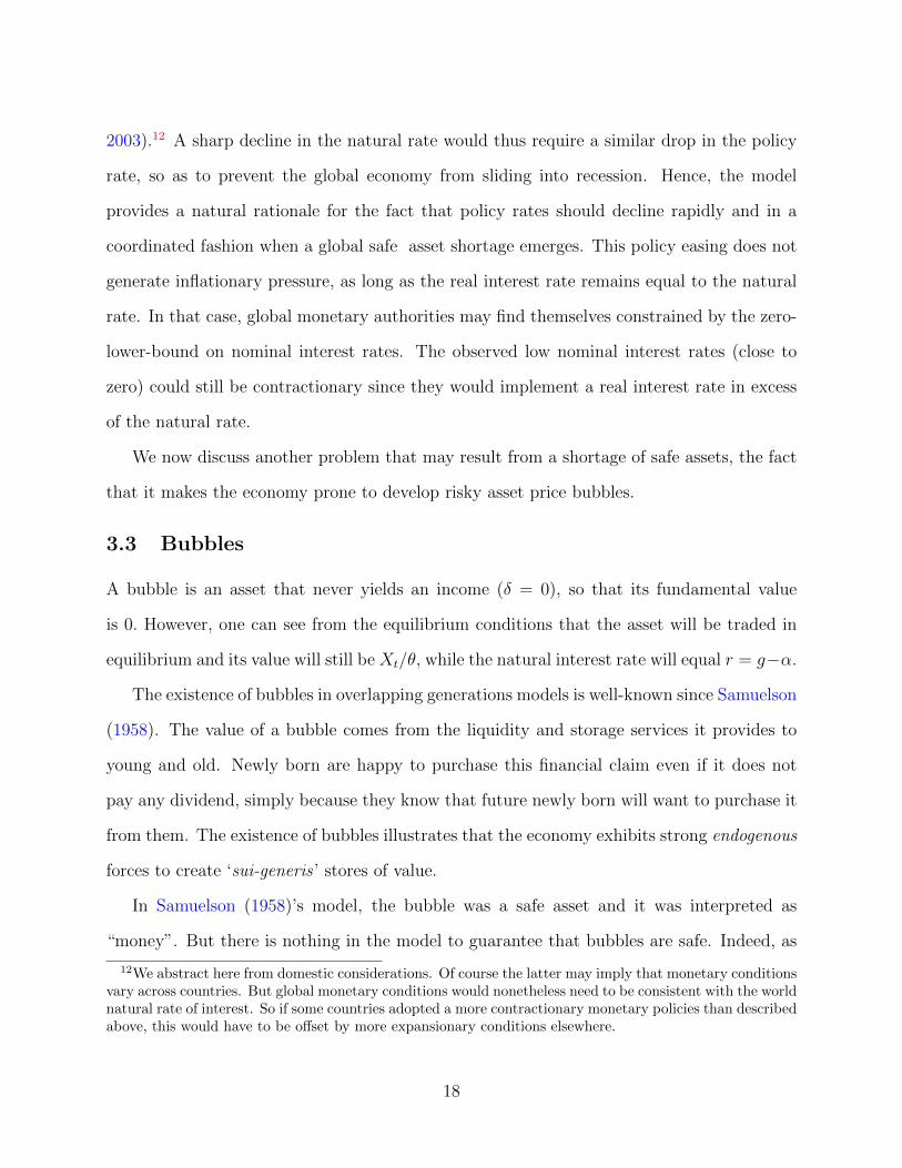
2003).12 A sharp decline in the natural rate would thus require a similar drop in the policy

rate, so as to prevent the global economy from sliding into recession. Hence, the model

provides a natural rationale for the fact that policy rates should decline rapidly and in a

coordinated fashion when a global safe asset shortage emerges. This policy easing does not

generate inflationary pressure, as long as the real interest rate remains equal to the natural

rate. In that case, global monetary authorities may find themselves constrained by the zero-

lower-bound on nominal interest rates. The observed low nominal interest rates (close to

zero) could still be contractionary since they would implement a real interest rate in excess

of the natural rate.

We now discuss another problem that may result from a shortage of safe assets, the fact

that it makes the economy prone to develop risky asset price bubbles.

3.3 Bubbles

A bubble is an asset that never yields an income (δ = 0), so that its fundamental value

is 0. However, one can see from the equilibrium conditions that the asset will be traded in

equilibrium and its value will still be Xt/θ, while the natural interest rate will equal r = g−α.

The existence of bubbles in overlapping generations models is well-known since Samuelson

(1958). The value of a bubble comes from the liquidity and storage services it provides to

young and old. Newly born are happy to purchase this financial claim even if it does not

pay any dividend, simply because they know that future newly born will want to purchase it

from them. The existence of bubbles illustrates that the economy exhibits strong endogenous

forces to create ‘sui-generis ’ stores of value.

In Samuelson (1958)’s model, the bubble was a safe asset and it was interpreted as

“money”. But there is nothing in the model to guarantee that bubbles are safe. Indeed, as

12We abstract here from domestic considerations. Of course the latter may imply that monetary conditionsvary across countries. But global monetary conditions would nonetheless need to be consistent with the worldnatural rate of interest. So if some countries adopted a more contractionary monetary policies than describedabove, this would have to be offset by more expansionary conditions elsewhere.

18

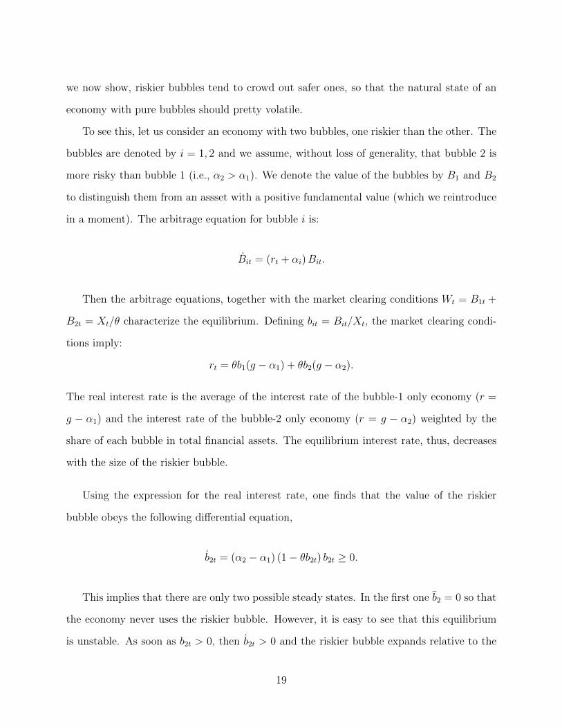
we now show, riskier bubbles tend to crowd out safer ones, so that the natural state of an

economy with pure bubbles should pretty volatile.

To see this, let us consider an economy with two bubbles, one riskier than the other. The

bubbles are denoted by i = 1, 2 and we assume, without loss of generality, that bubble 2 is

more risky than bubble 1 (i.e., α2 > α1). We denote the value of the bubbles by B1 and B2

to distinguish them from an assset with a positive fundamental value (which we reintroduce

in a moment). The arbitrage equation for bubble i is:

Bit = (rt + αi)Bit.

Then the arbitrage equations, together with the market clearing conditions Wt = B1t +

B2t = Xt/θ characterize the equilibrium. Defining bit = Bit/Xt, the market clearing condi-

tions imply:

rt = θb1(g − α1) + θb2(g − α2).

The real interest rate is the average of the interest rate of the bubble-1 only economy (r =

g − α1) and the interest rate of the bubble-2 only economy (r = g − α2) weighted by the

share of each bubble in total financial assets. The equilibrium interest rate, thus, decreases

with the size of the riskier bubble.

Using the expression for the real interest rate, one finds that the value of the riskier

bubble obeys the following differential equation,

b2t = (α2 − α1) (1− θb2t) b2t ≥ 0.

This implies that there are only two possible steady states. In the first one b2 = 0 so that

the economy never uses the riskier bubble. However, it is easy to see that this equilibrium

is unstable. As soon as b2t > 0, then b2t > 0 and the riskier bubble expands relative to the

19

safer one. The other steady state is b2 = 1/θ. That steady state is stable, meaning that all

paths starting with b2t > 0 converge to it. In that steady state, the riskier bubble crowds

out entirely the safer one, a sort of ‘Gresham-law ’ for bubbles.

Why does the riskier bubble crowd out the safer one? The answer is that the rate of

growth in the value of the riskier bubble needs to be higher, in equilibrium, to compensate

for the fact that it is more likely to collapse.13 It follows that the safer bubble becomes

smaller and smaller relative to the riskier one, and that its size in terms of GDP converges

to zero.

An economy with bubbles is likely to exhibit a very volatile boom-bust cycle in its asset

market assets. While asset crashes have no aggregate consequences in this model, it is easy

to imagine extensions where they would generate bank failures, financial instability, and real

volatilsity. So the risk that the financial sector might endogenously load on risky bubble

assets as stores of value should be a source of concern. Preventing the emergence of risky

bubbles is a reasonable objective for policymakers.

3.4 Safe asset prophylaxy

We now show that a sufficient supply of safe assets creates an environment in which it is

more difficult for bubbles to emerge. Safe assets have, so to speak, a prophylactic role: they

immunize the economy against the eruption of risky bubbles.

To see this, let us introduce a safe asset into an economy with bubbles. We now assume

that the economy has two assets, an asset V that has some fundamental value and virtually

no default risk (δ > 0 and α ' 0) and a bubble B with the opposite characteristics (δB = 0

and αB > 0). Since risky bubbles crowd out safer ones, one might be tempted to conclude

that the same will be true here: that the bubble will crowd out the safe asset. In fact, the

opposite is true: it is the safe asset that eliminates the bubble. Going through the same steps

13Remember that the collapse of the asset, in our model, means that the asset is transferred, not that itdisappears. The riskier bubble, thus, never disappears, but its owners are expropriated more often than forthe other bubble.

20

as before, the equilibrium conditions yield:

rt = g + δθ − α + (α− αB)θbt.

Then note that in the long term, the growth rate of the bubble must be smaller than the

growth rate of the economy, r + αB ≤ g. Otherwise the bubble would become infinitely

large relative to GDP, which is not possible since the demand for financial assets is a fixed

fraction of GDP. By backward induction, the bubble could not take off the ground. Using

the expression for the real interest rate, this implies that a bubble is possible only if

δθ ≤ (α− αB)(1− θb),

where b is the long-run bubble-value-to-GDP ratio. If α ≤ δθ, this expression cannot be

satisfied for positive values of αB and b. This expression can be satisfied for positive values

of b and αB only if α > δθ, and in this case bubbles can exist. Thus we have the following

result.14

Result 1. (Prophylactic role of safe a ssets) Bubble assets cannot exist in equilibrium if

there is a safe asset V such that α < θδ.

The condition α < θδ says that the risk in the safe asset must be small enough relative

to its fundamental value. If this condition is satisfied, the real interest rate r = g + δθ − α

is larger than the growth rate and bubbles cannot arise because the economy is dynamically

efficient. It is well-known from the literature that bubbles can exist only in environments

that are dynamically inefficient (i.e., in which the real interest rate is lower than the growth

rate).15 A safe asset makes the economy inhospitable to bubbles by making the economy

14See the appendix for a formal proof that fully characterizes the bubble dynamics.15The link between dynamic inefficiency and the possibility of rational bubbles is discussed at length in

the literature (e.g. Tirole, 1985, Blanchard and Weil, 2001, Ventura and Martin, 2011 and Farhi and Tirole,2011). Several recent contributions emphasize that it is possible for an economy to sustain bubble even ifthe economy is dynamically efficient. The key observation is that the market interest rate may be low (which

21

dynamically efficient, and it does so immediately, not asymptotically. As soon as the safe

asset is introduced, the interest rate rises sufficiently to destroy the value of the bubble asset.

This discussion offers a way to think about the different stages of the crisis in the real

world. Initially, the world experienced a decline in its global δ, due for instance to the

consequences of the Asian financial crisis, or the collapse in the dotcom bubble (see Caballero

et al. (2008) for an analysis of global imbalances along these lines). Interest rates declined.

With a low δ, the condition for the elimination of fragile bubbles (δθ > α) was not satisfied,

so ‘private label’ assets could emerge, both in the US and European financial sectors. The

low interest rates also fueled leverage, and therefore an increased demand for safe asset

‘internal’ to the financial sector.

With the onset of the financial crisis, some fragile bubbles collapsed and there was a

general re-assessment of the fragility of all financial claims, i.e., an across the board increase

in α. Increased financial fragility further reduced interest rates, opening the door to more

‘private label’ bubbles to emerge. In this context, the low-α assets, such as US Treasuries,

capture a premium.

3.5 Quantitative illustration

What is the appropriate supply of safe assets? If we take the model literally, the size of the

supply does not matter provided that the asset is perfectly safe (if α = 0, then the condition

α < δθ is satisfied for any δ). So in principle, the model says that it is possible even for a

tiny issuer of an assets (in the limit of δ = 0) to stabilize the global financial system as long

as α = 0. This is unrealistic as it implies that a country like Switzerland can underwrite

the entire supply of safe assets to the world. But this limit result does not survive in the

more realistic case where there is some incompressible amount of risk α for any asset, i.e.

is needed to sustain bubbles) while the social return to capital may be high (which is what is needed forproductive dynamic efficiency). The wedge between the market and the social rates of return to capital canin turn arise from financial or informational frictions. In short, one can study set-ups where bubbles canarise even if rates of return to capital exceed the growth rate. In these settings too, lower interest ratesincrease the likelihood that bubbles can emerge and survive.

22

α ≥ α > 0. Then the requirement that δθ > α has important implications for the ‘size’ of

the issuers.

Let us assume, for the sake of the discussion, that the safe asset is government debt

(more on this later). Suppose that the fiscal authority in country i issues debt with the

minimum level of risk α. The asset is a claim to future tax revenues τ iX i where τ i is the

implicit average rate of taxation and X i is the output of country i. If country i were under

autarky, the supply of this public asset would be enough to root out risky bubbles as long

as τ iθ > α. Suppose that this condition is satisfied. Now ask the following question: can

country i provide a sufficient quantity of safe assets for the global financial system? The

public asset of country i represents a claim to a share δ = τ iωi of the world output, where ωi

is the share of country i in world output: ωi = X i/X. The condition for financial stability

becomes

τ iωiθ > α.

This condition imposes a minimum size on country i : ωi > α/ (τ iθ) . For instance, with

an average tax rate of 20 percent, a marginal propensity to consume out of wealth θ of 5

percent and a lower bound probability of collapse of 0.2 percent per period (one collapse

every 500 periods), the minimum size of the supplier of safe assets is equal to 20 percent of

world output. Whether the asset risk is strictly equal to zero or simply close to zero can

make a large difference for the quantitative implications of the model.

Consequently, safe assets should provided by large economies with a sufficiently high fiscal

capacity (high τ iωi), or to put it differently, a deep and liquid market for Treasury securities

backed by the power to tax a substantial share of world output. This helps understand why

countries like the United States can play that role, while Switzerland or even Germany might

be too small. Whether the euro area can do it is a question that is discussed in the following

section.

23

4 Safe Assets and Central Banking

One lesson from the previous section is that it is important to maintain an appropriate

supply of safe assets for the stability of the global financial system. We discuss in this

section the role that central banks can play in maintaining this supply. As noted before,

central bank liabilities are the safe asset par excellence (in an environment with low and

stable inflation) since they are composed of currency or can be repaid by creating new

currency.16 By extension, a central bank can make any domestic-currency debt asset safe

by providing it with a “monetary backstop”, i.e., by committing to provide the issuer with

the currency required to repay the debt or to buy the asset itself at the no-default price. It

is difficult to think about the supply of safe assets, thus, without taking into account the

behavior of the central bank in a crisis.

One could indeed try and develop a history of central banking from the perspective of

the supply of safe assets. Central banks such as the Bank of England or the Banque de

France were originally created to be the banks of the sovereign and the managers of the

sovereign’s debt.17 Central banks then assumed the responsability of maintaining banking

stability during the nineteenth century, with the development of the lending-in-last-resort

doctrine by Walter Bagehot—a conception of central banking that inspired the creation of

the US Federal Reserve in 1913. Thus, one could argue (at the risk of oversimplifying)

that central banks were created to make government debt a safe (or at least, safer) asset,

and that this role was later extended to the liabilities of private banks. This would be an

oversimplification, of course, because central banks had other important goals, most notably

garanteeing the convertibility of their liabilities into gold or silver at a fixed parity. As a

result, the central banks’ ability to make the liabilities of the government and of other banks

16We are assuming that central bank liabilities are denominated in domestic currency. Conceivably acentral bank could default on its foreign-currency denominated liabilities.

17To quote the history page on the Bank of England web site, “The Bank of Eng-land was founded in 1694 to act as the Government’s banker and debt manager.”(http://www.bankofengland.co.uk/about/Pages/history)

24

safe had to be limited and conditional. For example, lending-in-last-resort was meant to

make banks’ liabilities safer against the risk of illiquidity but not that of insolvency.

After the link between money and commodity was severed in several steps during the

twentieth century, the focus of central banking theory shifted to the choice of the best nominal

anchor to replace gold. This effort culminated, at the end of the twentieth century, with a

view of central banking that is best represented (again, at the risk of oversimplifying) by

the inflation targeting doctrine. Inflation targeting focuses on the macroeconomic objectives

of central banks and does not seem to concern itself with the supply of safe assets. One

important theme of the last three decades of monetary theory is that the pursuit of low

inflation supposes that central banks do not use seigniorage to fill a gap in the government’s

intertemporal budget constraint, a regime that Sargent and Wallace (1981) called monetary

dominance. But monetary dominance, in the limit, may imply that the central bank let the

Treasury default if it is unable to roll over its debt, and thus to sacrifice the objective of

making government debt safe.

We see the tension between the pursuit of a nominal anchor and the supply of safe assets

now at play in the European debt crisis. Because of the time and the conditions in which

it was created, the European Central Bank (ECB) is perhaps the best incarnation of the

late 20th century view of central banking—even though the ECB is not, strictly speaking,

an inflation-targeting central bank. It is more likely in the euro area than elsewhere that

the monetary authorities will let the fiscal authorities default rather than taking the risk of

debt monetization and as a result, the debt of certain euro area governments has become less

safe. There are calls for the ECB to play its role of “lender of last resort” for governments,

based on a theory that the current government debt problems are self-fulfilling and not due

to insolvency (de Grauwe, 2011). However, whether a crisis is due to insolvency or illiquidity

is always a probabilistic judgement call, and one can never completely exclude that what

starts as lending in last resort later turns out to be the first step in the monetization of an

25

insolvent government.

We propose in this section a model that sheds light on these issues.18 The model features

a government that must roll over its debt and may be faced with a rollover crisis. The central

bank may avoid (or not) the default of the government by lending to it. The central bank’s

decision is taken in the context of a trade-off between maintaining the safe-asset status of

government debt and taking the risk of debt monetization.

4.1 Assumptions

The model has three periods, t = 0, 1, 2. The riskless real interest rate is normalized to zero

and investors are assumed to be risk-neutral. The government must roll over some debt d

in period 0 by issuing new debt that comes due in period 1 and bears a nominal interest

rate i. There is no fiscal income in period 1 so that the government must roll over its debt

(1 + i)d again until period 2. Debt is repaid with real fiscal income y in period 2, the level of

which is not known in period 0. A signal about the government’s solvency becomes public

in period 1, and for simplicity we assume that it is perfectly informative—that is, the level

of fiscal income, y, is revealed in period 1. The central bank can buy some government debt

in period 1 to avoid a default but this increases the price level in period 2. The price level

responds to an increase in money supply with a lag because of nominal stickiness.19

The nominal fiscal income in period 2 is p′y, where p′ is the price level in period 2

(remember that y is the real level of fiscal income). The price level in periods 0 and 1 is

normalized to p = 1. The price level in period 2, p′, is also equal to 1 if the central bank

sticks to its zero-inflation target but it could be higher if the central bank creates money to

rescue the government from a default.

There is a debt rollover crisis in period 1 if the fiscal income turns out to be insufficient

18The analysis in this section is based on Jeanne (2012b).19Alternatively, we could assume that the economy is in a liquidity trap in period 1, so that quantitative

easing is not immediately inflationary.

26

to repay the government debt conditional on zero inflation. In this case, two things may

happen: either the central bank buys the government’s debt to prevent a default (monetary

backstop), or it lets the government default. We take the probability that the central bank

lets the government default (conditional on a debt rollover crisis) as exogenous and denote

it by µ. Variable µ is a measure of monetary dominance.20 For simplicity, we assume that

there is no repayment in a default (the haircut is 100 percent).

The model is summarized by the following three equations:

(1 + i)d = d′ +m′ −m,

p′ =m′

m,

1

1 + i= Pr (y > d(1 + i)) + (1− µ) Pr (y < d(1 + i)) = 1− µF (d(1 + i)).

The first equation is the government’s budget constraint in period 1. In the absence

of fiscal income, the debt coming due in period 1, (1 + i)d, is rolled over either by issuing

new debt, d′, or by issuing new money, m′ − m. The second equation says that the price

level increases proportionately with money supply with a one-period lag. The third equation

gives the equilibrium value of the nominal interest rate i between period 0 and period 1.

The nominal interest rate could be higher than zero because of the default risk (which is

the only risk to consider since there is no inflation between period 0 and period 1). This

equation says that the period-0 value of a promise to pay one dollar in period 1, 1/(1 + i), is

equal to the probability that this dollar will be repaid. This probability, in turn, is equal to

the probability that the fiscal income is sufficient to repay the debt without money creation

(y > d(1 + i)) plus the probability that the government is rescued from a default by money

creation. In the second equality F (·) denotes the cumulative distribution function of y.

20In Jeanne (2012b) a distinction is drawn between hard monetary dominance (letting the governmentdefault in a rollover crisis) and soft monetary dominance (a proactive fiscal effort by the government toavoid a debt rollover crisis). Variable µ is a measure of hard monetary dominance.

27

If it is revealed in period 1 that y < (1 + i)d, the government cannot roll over its debt

without money creation.21 The central bank may then rescue the government from a default

by creating money to repay some of the debt. The monetary backstop avoids a default if

the fiscal income is sufficient to repay the residual debt that is rolled over between period 1

and period 2, that is if:

d′ ≤ y.

Assuming that the central bank creates the minimum amount of money to avoid a default

we have:

m′ = m+ (1 + i)d− y.

4.2 Lending in last resort

The advocates of stronger ECB intervention in government debt markets often present this

policy as a form of lending in last resort (see, e.g. de Grauwe, 2011). The underlying

diagnosis of the crisis is that it is essentially self-fulfilling and due to an adverse feedback

loop in which high spreads lead to unsustainable debt dynamics—a type of self-fulfilling

crisis that was modeled by Calvo (1988).

Lending in last resort to governments is easy to rationalize in our model. To see this,

note that the nominal interest rate i satisfies the following equation,

[1− µF (d(1 + i))] (1 + i) = 1. (1)

Let us assume that the government is solvent in period 0, in the sense that it is able to

repay its debt even for the lowest realization of its fiscal income if it rolls over its debt at the

21The government is solvent if the nominal debt repayment is lower than the nominal fiscal income inperiod 2, i.e., (1 + i′)d′ ≤ p′y,where i′ is the nominal interest rate between period 1 and period 2. The realinterest rate being equal to zero, the Fisher equation implies 1 + i′ = p′/p = p′. Using this equation andd′ = (1 + i)d to substitute i′ and d′ out of (1 + i′)d′ ≤ p′y shows that the government can roll over its debtwithout money creation only if d(1 + i) ≤ y.

28

riskless interest rate (F (d) = 0). Then i = 0 is a solution of equation (1), i.e., there is an

equilibrium in which the government rolls over its debt at a zero interest rate and remains

solvent without debt monetization. This may not be the only equilibrium, however. In the

absence of monetary backstop (µ = 1), the equation above could also admit another solution

with a positive interest rate i > 0 because its left-hand side may be decreasing with i. The

intuition for this multiplicity is exactly the same as in Calvo (1988)’s model of self-fulfilling

debt crises. A higher level of interest rate implies a higher burden of repayment in the future,

which increases the probability of default and thus becomes self-validating.

The bad equilibrium disappears if the central bank pins down the interest rate spread to

zero by committting to provide a monetary backstop to a government debt crisis (µ = 0).

The only solution to equation (1), then becomes i = 0. The monetary backstop removes

the default risk without creating an inflation risk. The default risk is not replaced by an

inflation risk because—we assume—debt monetization leads to inflation with a one-period

lag and so does not generate an inflation risk premium between period 0 and period 1. The

promise to monetize debt removes the bad equilibrium and never has to be implemented in

the good equilibrium. As a result, there is neither a default risk nor an inflation risk in the

good equilibrium. Lending in last resort delivers a policymaking “free lunch.”

The case with F (d) = 0 thus delivers a stark conclusion. By providing a monetary

backstop, the central bank can make government debt a safe asset in all dimensions: it

removes the default risk in government debt without creating an inflation risk. The monetary

backstop, in this case, can truly be called a form of lending in last resort.

4.3 The trade-off between default risk and inflation risk

The case F (d) = 0 delivers stark conclusions but it may be more realistic to consider the

case where the government is not solvent with probability 100 percent conditional on not

paying a spread, i.e., where F (d) is perhaps small but not strictly equal to zero. In this case,

29

whether or not to provide the monetary backstop involves a trade-off between default risk

and inflation risk. We explore in this section the terms of this trade-off.

Let us respectively denote by Pdef and Pinf the probability of default and the probability

of inflation viewed from period 0. Setting d = 1 to alleviate the algebra, we have

Pdef =µF (1 + i),

Pinf = (1− µ)F (1 + i).

Using equation (1) the interest rate on government debt can be defined as an increasing

function of the probability that the central bank will not provide a monetary backstop,22

i = i(+µ).

Increasing µ raises the probability that there is a debt rollover crisis with either default

or inflation,

d(Pdef + Pinf)

dµ= f(1 + i)i′(µ) > 0,

where f(·) = F ′(·) is the probability distribution function of y.

It would be wrong, thus, to assume that the monetary backstop simply replaces the risk

of default by a risk of inflation. Enhancing the monetary backstop (reducing µ) raises the

probability of inflation by less than it reduces the probability of default because this lowers

the probability of the event leading to either default or inflation (a debt rollover crisis).

Conceivably, reducing µ could lower the probabilities of both default and inflation. This is

the case if dPinf/dµ > 0, that is if

i′(µ) >F (1 + i)

(1− µ)f(1 + i).

22i is increasing with µ if the l.h.s. of equation (1) is increasing with i, i.e., if the equilibrium is on theefficient part of the debt Laffer curve. This must be the case in a good equilibrium.

30

If the interest rate spread is very responsive to the probability of monetary backstop, then

raising this probability might reduce the risks of both default and inflation.

To illustrate, Figure 8 shows how the probabilities of default (blue line) and inflation

(green line) depend on the probability of monetary backstop, α = 1 − µ. To construct the

figure, the initial debt was set to d = 1, and the fiscal income was assumed to be normally

distributed with mean 1.3 and standard deviation 0.2, implying that the government is

solvent with probability 93 percent if it does not pay a default risk premium on its debt.

However, in the absence of a monetary backstop (µ = 1) the government has to pay a

default risk premium that raises the debt repayment and endogenously reduces its solvency.

For these parameter values, the government is in fact unable to refinance its debt in period 0

in the absence of monetary backstop, and must default with probability 1. The probability

of monetary backstop must be higher than 43 percent for the government to be able to

roll over its debt in period 0. When this is the case, the probability of inflation remains

relatively small. For a full monetary backstop (µ = 0), the probability of inflation is equal to

the probability that the government is insolvent conditional on not paying a risk premium,

which is about 7 percent.

The monetary backstop, thus, does not simply replace a bad outcome (default) by another

(inflation), it reduces the probability of a bad outcome altogether by allowing the government

to roll over its debt at a low interest rate and mitigating the risk of explosive debt dynamics.

A monetary backstop replaces a high probability of default by a low probability of inflation,

and might be a necessary condition to maintain the safe asset status for government debt.

4.4 Incentives

The model, as it stands, does not capture what is perhaps the main argument against

providing a monetary backstop to the government debt market, which is that it gives bad

fiscal incentives to governments. We now look more closely into this argument.

31

Let us assume that the economy pays a welfare cost Cdef for a government default and

a cost Cinf for monetizing the debt. The cost of government default could involve a banking

crisis, a capital flight or a loss of reputation.23 The costs of monetizing the debt are not

very different, especially if the inflation rate is high and the size of the debt to be monetized

is such that inflation should be accompanied by banking and financial repression.24 Jeanne

(2012b) argues that since government debt in advanced economies is a large multiple of base

money, the welfare cost of monetization would indeed be high and perhaps not much smaller

than that of an outright default.

Viewed from period 0, the expected welfare cost of either default or inflation (i.e. the

expected welfare cost of a debt rollover crisis) is given by

C =PdefCdef + PinfCinf ,

=F (1 + i) [Cinf + µ(Cdef − Cinf)] .

In order to study fiscal incentives, let us assume that the government has the choice in period

0 between a “good” fiscal policy and a “bad” fiscal policy. Fiscal income tends to be higher

with the good policy than with the bad one. More formally, the probability that fiscal income

falls below any level is higher with the bad fiscal policy, that is Fb(y) > Fg(y) for any y. The

choice of the fiscal policy is made after the government has borrowed at interest rate i.

Assuming that the government is benevolent, the incentives to implement good fiscal

policy are captured by the welfare cost difference,

Cb − Cg = [Fb(1 + i)− Fg(1 + i)] [Cinf + µ(Cdef − Cinf)] , (2)

where Cg and Cb are the expected welfare cost of a debt rollover crisis under the good fiscal

23There is a large literature on the costs of defaulting on sovereign debt. See Borensztein and Panizza(2009) for a review.

24See Reinhart and Sbrancia, 2011.

32

policy and the bad fiscal policy respectively.

If defaulting is more costly than monetizing the debt, the second factor on the right-hand

side of equation (2) is increasing with µ. That is, monetary dominance gives the government

an incentive to implement the good fiscal policy. This is the effect that the opponents of

the monetary backstop have in mind. However, there is another effect involving the nominal

interest rate. The monetary backstop could enhance the fiscal incentives if it reduces the

interest rate more under the good fiscal policy than under the bad one.25 If the cost difference

Cdef − Cinf is small, it is not clear which effect dominates.

The model also explains why the relationship beween monetary policy and government

debt is more problematic in the euro area than elsewhere. In currency areas where there is

one single fiscal authority (such as the US, the UK or Japan), this auhority fully internalizes

the welfare costs of debt monetization. In the euro area, by contrast, the cost of debt

monetization are shared among the member countries. This may be captured in the model

by assuming that the cost of debt monetization is Cinf/n instead of Cinf where n is the

number of member countries. This reduces the right-hand side of equation (2), an effect

that may be offset by increasing µ, i.e., by enhancing monetary dominance. That is, the

incentives to choose a good fiscal policy are weakened in a currency union, and it becomes

more important to keep the incentives aligned by not providing a monetary backstop.

Another implication of the model is that it might be more desirable to provide the

monetary backstop for government debt than for private debt. The reason is that private

borrowers, being small relative to the whole economy, do not internalize their contribution to

the monetization risk and are therefore more likely to undertake excessive risk in reponse to

the monetary backstop. More formally, for a small private borrower the relevant action is an

effort that improves the future cash flow. Denoting with a lower-case letter the variables of a

small atomistic borrower, the welfare benefit of making the effort is the same as in equation

25The monetary backstop enhances the fiscal incentives if Fb(1 + i)− Fg(1 + i) is decreasing with i. Thevariations of Fb(1 + i)− Fg(1 + i) with i are not signed in general.

33

(2) but excluding the cost of inflation, which is taken as exogenous by the borrower,

cb − cg = [Fb(1 + i)− Fg(1 + i)]µcdef .

We observe that the incentives to avoid a default are directly proportional to the monetary

dominance index and disappear if µ = 0. This is a classical example of moral hazard induced

by a financial safety net. In this case, furthermore, the financial safety net is endogenous

to the actions of the private borrowers who do not internalize their collective impact on

policy.26 By contrast, the government, as a large borrower that cares about social welfare,

internalizes the welfare cost of debt monetization when setting fiscal policy.

4.5 Discussion

For government debt to remain a safe asset, the government must remain solvent. This

leaves open the question of how the monetary authorities can help the fiscal authorities to

st ay solvent. The conventional view is that the monetary authorities should focus entirely

on price stability and let the government adjust fiscal policy conditional on low seigniorage.

The alternative would be to monetize the government’s debt, which would replace a bad

outcome (default) by a worse one (high inflation). This view of the relationship between

central banking and government debt is widely accepted in policy circles and it is supported

by the academic literature on monetary policy. But it implies, in the limit, that the monetary

authorities should stand ready to let the government default in the event of a debt rollover

crisis.

The model that we have just presented suggests that the conventional view misses a few

subtle but important things about the relationship between central banking and government

debt. First, in a situation with multiple equilibria, a promise by the central bank to backstop

a debt rollover crisis removes the bad equilibrium without creating an inflationary risk. The

26This is a version of the common agency problem modeled by Tirole (2003).

34

central bank’s monetary backstop makes government debt default-free without making it

more risky in terms of inflation.

Second, even if the government is not solvent for sure conditional on the monetary back-

stop, the trade-off between the default risk and the inflation risk might be such that it is

possible to reduce the default risk a lot at the cost of a small risk of inflation. The monetary

backstop stabilizes the dynamics of government debt by preventing negative shocks from

raising the interest rate and the ensuing feedback loop between high interest rates, rising

debt and pessimistic expectations. Given the terms of the trade-off, it is not clear a priori

that it is preferable to minimize the risk of inflation rather than that of default.

Coming back to the crisis, one puzzle is why the government debt turmoil started in the

euro area rather than the US, the UK or Japan even though the fiscal fundamentals seemed

better on average in the euro area than in the latter countries before the crisis.27 Although

other factors are certainly at play, we would suggest that this is due primarily to a difference

in the relationship between central banking and government debt. There is an expectation

in most economies (including those with an inflation-targeting regime) that the central bank

would intervene to avoid a government default in a rollover crisis. This expectation does

not exist in the euro area because of the way it was designed. As we have argued, there

are reasons that the euro area was designed in this way: in particular, the multiplicity of

fiscal authorities makes it more important to enforce monetary dominance in the euro area

than elsewhere—at least until the appropriate fiscal incentives are provided by mechanisms

other than spreads on government debt. But other things equal, this puts the euro area at

a disadvantage in the production of safe assets.

What is the implication for the future of safe assets? One (pessimistic) view is that the

euro area debt crisis reflects a trend of safe asset extinction. Private-label safe assets became

27As shown in Jeanne (2012b), in 2009 the levels of government debt and of primary deficit relative toGDP were lower on average in the euro area than in the US, the UK or Japan (which were comparable tothe average worse four or five countries in the euro area).

35

unsafe, after which it was the turn of advanced economies government debt, starting (but

this is only the beginning) in the euro area. We are skeptical that these two events (the

US mortgage crisis and the euro area government debt crisis) should be extrapolated in this

way. The euro area debt crisis is generated to a large extent by factors that are specific to

the euro area and come from the way it was designed. In most advanced economies outside

the euro area, the attitude of central banks toward government debt is such as to ensure a

low default risk at the same time as a low inflation risk.

Finally, the problem with the supply of safe assets does not seem to be that the quantity

was insufficient, but rather that the definition of safe assets has been elusive and shifting.

In the old times, safe assets were defined as central bank liabilities (cash) and government

debt. With securitization and tranching, new classes of assets came to be used as safe

assets (e.g., senior tranches of MBS) in the US, but they turned out to be not so safe. Their

fragility comes from the unavoidable fact that private assets are poorly designed to withstand

aggregate shocks. More recently in Europe, certain government debts have lost the status

of safe assets. As a result of those shifting lines of demarcation, the definition of what truly

constitutes a safe asset became blurry, leading to a sentiment that no asset is safe any more.

Against this backdrop, we would argue in favor of coming back to the basics. It is of

the essence of a safe asset that it should not become unsafe. The supply of safe assets has

a key impact on the the financial sector and the real economy and so the definition of the

safe asset universe should not be left entirely to the private sector. The authorities should

commit themselves to a clear definition of safe assets and back it with a policy regime that

makes those assets credibly safe. Claims on the private sector are inherently risky and should

stay so to limit moral hazard: for this reason they may not provide a good basis to produce

safe assets. Besides money, government debt remains the best candidate for the status of

safe asset.

36

5 Safe Assets in the Global Economy

The previous analysis has a number of implications for the global economy. First, it suggests

that global banking will naturally take place in the currency that offers an appropriate

supply of safe assets. This role is fulfilled now primarily by the US dollar. As is explored in

great detail in Bruno and Shin (2012), this implies that global banks play a powerful role in

transmitting dollar monetary and credit conditions to the rest of the world.

Second, we have argued that there are important distinctions to be made between inside

and outside liquidity and between public and private liquidity. In tranquil times, these dif-

ferent forms of liquidity are close substitutes and trade at similar prices. In times of global

stress, however, private and inside liquidity dry up, as counterparty risk rises. The only

relevant form of liquidity comes from the public sector, through liquidity injections of the

monetary authorities, or the injection of public funds in troubled financial institutions. Our

analysis in section 3 indicates that the disappearance of ‘safe assets’ can unleash financial in-

stability as the global economy searches for alternate stores of value. The general equilibrium

signature of a decline in the supply of safe assets is a decrease in real interest rates. While

this mechanism is in general stabilizing (increasing the supply of existing stores of value),

it can push the economy in a fragile state where financial instability increases further. The

solution, we argued, is to ensure that the world economy is supplied with a sufficient quan-

tity of public safe assets. Section 4 argues that this requires a careful coordination between

monetary and fiscal policy, to ensure that public assets remain safe, even in the face of a

global crisis.

One could imagine a future where this global provision of safe assets is decentralized.28

Under the ‘house in order’ doctrine, each major economy could ensure the safety of their

domestically-issued public debt instruments through sound fiscal policy –ensuring that the

28See Farhi, Gourinchas and Rey (2011) for a more in-depth analysis.

37

present value of future real primary surpluses is sufficient to cover outstanding real liabilities

in most states of the world– and monetary/fiscal coordination –immunizing public debt

against roll-over crisis and extreme events. In such a ‘multi-polar’ world, the global supply

of safe assets would grow more or less in line with the world economy, ensuring a globally

adequate provision of safe assets, and the excess return accruing to the issuers of the safe

assets are likely to be more evenly shared. A corollary is that we can expect the central role

of the dollar to eventually decline.

We are far, however, from such an environment. Of the four major world economies –the

U.S., the Eurozone, Japan and China– only two – the U.S. and Japan– are currently providing

global safe (and public) assets, with the addition of smaller economies such as Switzerland,

Germany or to some extent the U.K.. China’s current state of financial development and

closed capital account imply that it is far from being able to play that role. As for the

Eurozone, we discussed in the previous section how the common pool problem that lies at

the core of that region’s crisis prevents the European Central Bank from offering an effective

backstop to publicly issued liabilities, opening the door to liquidity and solvency sovereign

crises. In the short to medium term, it is clear that the fiscal-monetary nexus seems more

conducive to the production of safe assets in the US than in the euro area. One corollary

is that the role of the dollar is likely to be comforted, rather than weakened, by the latest

crisis. The current environment of safe asset scarcity, low real interest rates, and financial

volatility is therefore here to last.

Going forward, the global scarcity of safe assets is bound to increase as the global demand

for safe assets—-tied to global economic growth—-outstrips the supply—tied to US economic

growth and fiscal sustainability. This is the modern version of Triffin (1960)’s dilemma. This

problem might be solved, in the long run, by the emergence of new safe assets. One area of

uncertainty, however, is how multiple safe assets will compete on a global stage. We have

outlined above one possibility: that by increasing the supply of safe assets, a multipolar

38

world will remove some sources of financial instability. But the virtuous feedback loop that

supports the status of safe assets may also turn vicious, and the arbitrage between safe

assets might generate rather than reduce volatility. In other words, the transition to a more

multipolar world may not be monotonous, nor smooth, if and when it occurs. A multipolar

world may therefore itself need a global backstop. As Farhi et al. (2011) discuss, this is

a role that could be played by the International Monetary Fund, in coordination with the

monetary authorities or Treasuries of the global issuers of safe assets.

39

References

Bernanke, Ben, “The Global Saving Glut and the U.S. Current Account Deficit,” SandridgeLecture, Virginia Association of Economics, Richmond, Virginia, Federal Reserve BoardMarch 2005.

Bernanke, Ben S., Carol Bertaut, Laurie Pounder DeMarco, and Steven Kamin,“International capital flows and the returns to safe assets in the United States, 2003-2007,”International Finance Discussion Papers 1014, Board of Governors of the Federal ReserveSystem 2011.

BIS, BIS Annual Report: Monetary Policy Challenges Ahead, Basle, Switzerland: Bank forInternational Settlements, 2011.

Blanchard, Olivier and Philippe Weil, “Dynamic Efficiency, the Riskless Rate, andDebt Ponzi Games under Uncertainty,” The B.E. Journal of Macroeconomics, 2001, 0 (2).

Borensztein, Eduardo and Ugo Panizza, “The Costs of Sovereign Default,” IMF StaffPapers, 2009, 56 (4), 683–741.

Brunnermeier, Markus K., “Deciphering the 2007-08 Liduidity and Credit Crunch,”Journal of Economic Perspectives, 2009.

Bruno, Valentina and Hyun Song Shin, “Capital Flows, Cross-Border Banking andGlobal Liquidity,” mimeo Princeton University March 2012.

Caballero, Ricardo J., “Sudden Financial Arrest,” IMF Economic Review, 2010, 58 (1),6–36.

, “Understanding the global turmoil: It’s the general equilibrium, stupid,” http://www.

voxeu.org/index.php?q=node/5077 May 2010.

, Emmanuel Farhi, and Pierre-Olivier Gourinchas, “An Equilibrium Model of“Global Imbalances” and Low Interest Rates,” American Economic Review, March 2008,98 (1), 358–93.

Calvo, Guillermo A, “Servicing the Public Debt: The Role of Expectations,” AmericanEconomic Review, September 1988, 78 (4), 647–61.

Credit Suisse, 2012 Global Outlook: Piecing Together or Falling to Pieces, December 2011.

Dang, Tri Vi, Gary Gorton, and Bengt Holmstrom, “Financial Crises and the Opti-mality of Debt for Liquidity Provision,” mimeo MIT May 2010.

de Grauwe, Paul, “Managing a Fragile Eurozone,” CESifo Forum, 2011, 12 (2), 40–45.

Diamond, Douglas W. and Philip H. Dybvig, “Bank Runs, Deposit Insurance, andLiquidity,” Journal of Political Economy, 1983, 91 (3), 401–19.

40

and Raghuram G. Rajan, “Illiquid Banks, Financial Stability, and Interest RatePolicy,” NBER Working Papers 16994, National Bureau of Economic Research, Inc 2011.

Eggertsson, Gauti and Paul Krugman, “Debt, Deleveraging, and the Liquidity Trap,”Quarterly Journal of Economics, forthcoming 2012.

Farhi, Emmanuel and Jean Tirole, “Bubbly Liquidity,” NBER Working Papers 16750,National Bureau of Economic Research, Inc January 2011.

, Pierre-Olivier Gourinchas, and Helene Rey, Reforming the International MonetarySystem, London, UK: Center for Economic Policy Research, 2011.

Garcia, Cardiff, “The decline of ‘safe’ assets,” The Financial Times, Decem-ber 05, 2011, http: // ftalphaville. ft. com/ blog/ 2011/ 12/ 05/ 778301/

the-decline-of-safe-assets/ .

Guerrieri, Veronica and Guido Lorenzoni, “Credit Crises, Precautionary Savings, andthe Liquidity Trap,” NBER Working Papers 17583 November 2011.

Holmstrom, Bengt, “Comments on “The Panic of 2007”,” in “Maintaining Stability in aChanging Financial System” Jackson Hole Conference, Kansas City Federal Reserve BankKansas City, MO 2008, pp. 263–273.

and Jean Tirole, “Private and Public Supply of Liquidity,” Journal of Political Econ-omy, February 1998, 106 (1), 1–40.

International Monetary Fund, Global Financial Stability Report: The Quest for LastingStability, Washington D.C.: International Monetary Fund, April 2012.

Jeanne, Olivier, “The Dollar and its Discontents,” NBER Working Papers 18143, NationalBureau of Economic Research, Inc June 2012.

, “Monetary Dominance and Government Default,” Financial Stability Review, 2012, 16,143–150.

Nakagawa, Shinobu and Yosuke Yasui, “A note on Japanese household debt: inter-national comparison and implications for financial stability,” in Bank for InternationalSettlements, ed., Household debt: implications for monetary policy and financial stability,Vol. 46, Bank for International Settlements, 2009, pp. 75–82.

Pagano, Marco, “Endogenous Market Thinness and Stock Price Volatility,” Review ofEconomic Studies, 1989, 56 (2), 269–87.

Reinhart, Carmen M. and M. Belen Sbrancia, “The Liquidation of Government Debt,”Working Paper 16893, National Bureau of Economic Research March 2011.

Samuelson, Paul A., “An Exact Consumption-Loan Model of Interest with or without theSocial Contrivance of Money,” Journal of Political Economy, 1958, 66.

41

Sargent, Thomas J. and Neil Wallace, “Some unpleasant monetarist arithmetic,” Quar-terly Review, 1981, (Fall), v. 5, no. 3.

Shin, Hyun Song, “Global Banking Glut and Loan Risk Premium,” IMF Economic Review,June 2012, 60 (2). Mundell Fleming Lecture, Annual Research Conference, InternationalMonetary Fund.

Tirole, Jean, “Asset Bubbles and Overlapping Generations,” Econometrica, 1985, 53 (6),1499–1528.

, “Inefficient Foreign Borrowing: A Dual- and Common-Agency Perspective,” AmericanEconomic Review, 2003, 93 (5), 1678–1702.

Triffin, Robert, Gold and the dollar crisis; the future of convertibility, New Haven: YaleUniversity Press, 1960.

Ventura, Jaume and Alberto Martin, “Economic growth with bubbles,” EconomicsWorking Papers, Department of Economics and Business, Universitat Pompeu Fabra 2011.

Woodford, Michael, Interest and Prices: Interest and Prices: Foundations of a Theory ofMonetary Policy, Princeton NJ: Princeton University Press, 2003.

42

Appendices

A Proof of Result 1.

The dynamic equation for the bubble can be written

·bt =

·Bt

Xt− gbt = (rt + αB − g)bt = (αB − α)θ

(1

θ+

δ

αB − α− bt

)bt. (A.1)

This equation shows that if αB > α, starting from any positive value b0 the bubble value convergestowards

b =1

θ+

δ

αB − α.

But this means that the bubble value will exceed 1/θ, which is not possible since the demand forthe store of value is inelastically fixed at 1/θ. Thus, it is not possible to have a bubble with αB > α.

If α = αB then equation (A.1) becomes·bt = δθbt, and there is no admissible solution except

bt = 0.Finally, if αB < α, the dynamic equation for the bubble can be rewritten

·bt = (α− αB)θ

[bt −

(1

θ− δ

α− αB

)]bt.

The only possible solution is that the bubble value stays constant and equal to

b =1

θ− δ

α− αB.

Any different initial value would lead to the bubble value diverging to plus or minus infinity, whichis not possible since the bubble value must stay positive and bounded by 1/θ. For this bubble valueto be positive one must have αB ≤ α − δθ. The default probability must be lower on the bubblethan on the safe asset.

B Details on Data Construction.

• Figure 3:

– Real sector demand for safe assets: from Flow of Funds Table L.100 (Householdsand NonProfit Organization) and Table L.101 (Nonfinancial Business). Householdsafe assets defined as the sum of Deposits (FL154000025), credit market instruments(FL154004005) minus Corporate and foreign bonds (FL15363005), Syndicated loans(FL153069803) and Mortgages asset (FL153065005). Nonfinancial business safe as-sets defined as the sum of Foreign deposits (FL103091003), checkable deposits andcurrency (FL143020005), Time and saving deposits (FL143030005), Money market mu-tual fund shares (FL143034005), Security repos (FL102050003) and Credit market in-struments (FL144004005) minus Mortgages asset (FL143065005) and Consumer credit(FL143066005).

– Real sector holdings of government securities from Flow of Funds Table L.100 andTable L.101, defined as sum of household holdings of Treasury securities including sav-ing bonds (FL153061505), household holdings of Municipal securities (FL153062005),nonfinancial business holdings of Treasury securities (FL143061105) and nonfinancialholdings of Municipal Securities (FL143062005).

43

• Figure 4

– United States: see Figure 3

– United Kingdom: from Blue Book 2010, sum of households and non financial businesssafe asset holdings defined as:

∗ Household and non-profit organizations: ESA sectors S.14 and S.15 unconsolidated,sum of Currency and deposits (AF.2), money market instruments (MMI) issuedby UK central government (AF.3311), UK local authority bills (AF.3312), MMIissued by UK monetary and financial institutions (AF.3315), MMI issued by otherUK residents (AF.3316), bonds issued by the UK central government (AF.3321),UK local authority bonds (AF.3322).

∗ non financial business: ESA sector S.11 unconsolidated, sum currency and deposits(AF.2), MMI issued by UK general government (AF.3311), UK local authoritybills (AF.3312), MMI issued by UK monetary and financial institutions (AF.3315),MMI issued by other UK residents (AF.3316), MMIS issued by the rest of theworld (AF.3319), bonds issued by the UK central government (AF.3321), UK localauthority bonds (AF.3322).

– Germany and France: from OECD Financial Balance Sheets (non-consolidated); sum ofcurrency and deposits (SAF2ASNC) and Securities other than shares, except financialderivatives (SAF33ASNC) for Households and nonprofit (sector S.14 and S.15) and nonfinancial business (sector S.11).

– European Area: from European Central Bank flow of funds.

∗ Households and non-profit: sum of currency and deposits, securities other thanshares, except financial derivatives, shares and other equity, minus shares and otherequity excluding money market mutual funds

∗ Non-financial business: sum of currency and deposits and Securities other thanshares, except financial derivatives.

– Japan: from Bank of Japan Flow of Funds. Constructed as sum of :

∗ Households and Non-profit: sum of Currency and deposits (FFYS430A150 &FFYS440A100), Treasury discount bills (FFYS440A310), central government secu-rities and FILP bonds (FFYS430A311 & FFYS440A311), local government securi-ties (FFYS430A312 & FFYS440A312), public corporations securities (FFYS430A313& FFYS440A313)

∗ Nonfinancial corporations: sum of Currency and deposits (FFYS410A100), De-posits with the Fiscal Loan Fund (FFYS410A190), Bills purchased and sold (FFYS410A230),repos (FFYS410A280), Treasury discount bills (FFYS410A310), Central gov. secu-rities and FILP bonds (FFYS410A311), local government securities (FFYS410A312),public corporation securities (FFYS410A313) and commercial paper (FFYS410A317).

• Figure 5:

– Holdings of official safe assets by rest of the world from Flow of Funds Table L.106(Rest of the World) sum of Special Drawing Rights (FL313111303), Treasury securi-ties (FL263061105), Municipal securities (FL263062003) and Table L.204 (Checkabledeposits and currency) Rest of the world currency;

– Holdings of safe assets by rest of the world from Flow of Funds Table L.106 (Rest of theWorld) sum of SDR (FL313111303), US checkable deposits and currency (FL263020005),US time and saving deposits (FL263030005), US money market fund mutual shares

44

(FL263034003), repos (FL262050003), commercial paper (FL263069103), Treasury se-curities (FL263061105), agency and GSE-backed securities (FL263061705), municipalsecurities (FL263062003) and from Table L.203 (Net interbank transactions) sum ofUS chartered depository institutions interbank transactions due to foreign affiliates(FL763192603) and foreign banking offices interbank transactions due to foreign affili-ates (FL753192603).

• Figure 6:

– Real sector demand for safe assets from financial sector as in Figure [safe real assets].

– Real sector supply of illiquid assets to financial sector: from Flow of Funds TableL.100 (Households and NonProfit Organizations), Table L.101 (Nonfinancial Business)and Table L.216 (Other loans and advances). Household supply defined as Creditmarket instruments liability (FL154104005) minus Municipal securities (FL163162003)and Other loans and advances (FL153169005). Nonfinancial Business supply definedas the sum of Commercial paper liabilities (FL103169100), Bank loans (FL143168005),Other loans (FL143169005) and Mortgages (FL143165005), minus U.S. governmentloans to nonfinancial corporate business (FL103169205) and nonfinancial noncorporatebusiness (FL113169205).

• Figure 7:

– From Flow of Funds Table L.107 (Financial Business) sum of Treasury securities (FL793061105)and Municipal securities (FL793062005) minus Table L.108 (Monetary Authority) Trea-sury securities (FL713061100), Table L.117 (State and Local Government EmployeeRetirement Funds) Municipal securities (FL223062003)

– From Flow of Funds Table L.108 (Monetary authority) sum of Depository institutionsreserve (FL713113003) and vault cash of depository institutions (FL763025005).

45

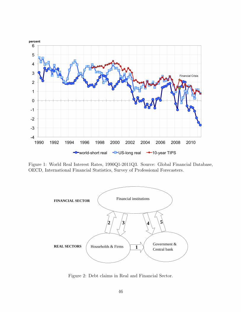
Financial Crisis

-4

-3

-2

-1

0

1

2

3

4

5

6

1990 1992 1994 1996 1998 2000 2002 2004 2006 2008 2010

percent

world-short real US-long real 10-year TIPS

Figure 1: World Real Interest Rates, 1990Q1-2011Q3. Source: Global Financial Database,OECD, International Financial Statistics, Survey of Professional Forecasters.

REAL SECTORS

FINANCIAL SECTOR

Households & Firms 1

3 4

Financial institutions

Government & Central bank

2 5

Figure 2: Debt claims in Real and Financial Sector.

46

0

20

40

60

80

100

120

percent US Real Sector* - Holding of Safe Assets as % of US GDP

safe real private sector holdings of govt. securities holdings of financial sector securities

*Households and Non-Profit Organizations + Non-financial Corporations

Figure 3: Holdings of Safe Assets by US Households and US Non Financial Business Sectors.Percent of US GDP. Source: Flow of Funds Accounts. See appendix B

47

0

50

100

150

200

250

percent Real Sector - Holding of Safe Assets as % of GDP

United Kingdom United States Japan Euro Area France Germany

*Households and Non-Profit Organizations + Non-financial Corporations

Figure 4: Holdings of Safe Assets by Households and Non Financial Business Sectors inJapan, the UK, Germany, France and the euro area. Percent of GDP. Source: Flow of FundsAccounts. See appendix B

48

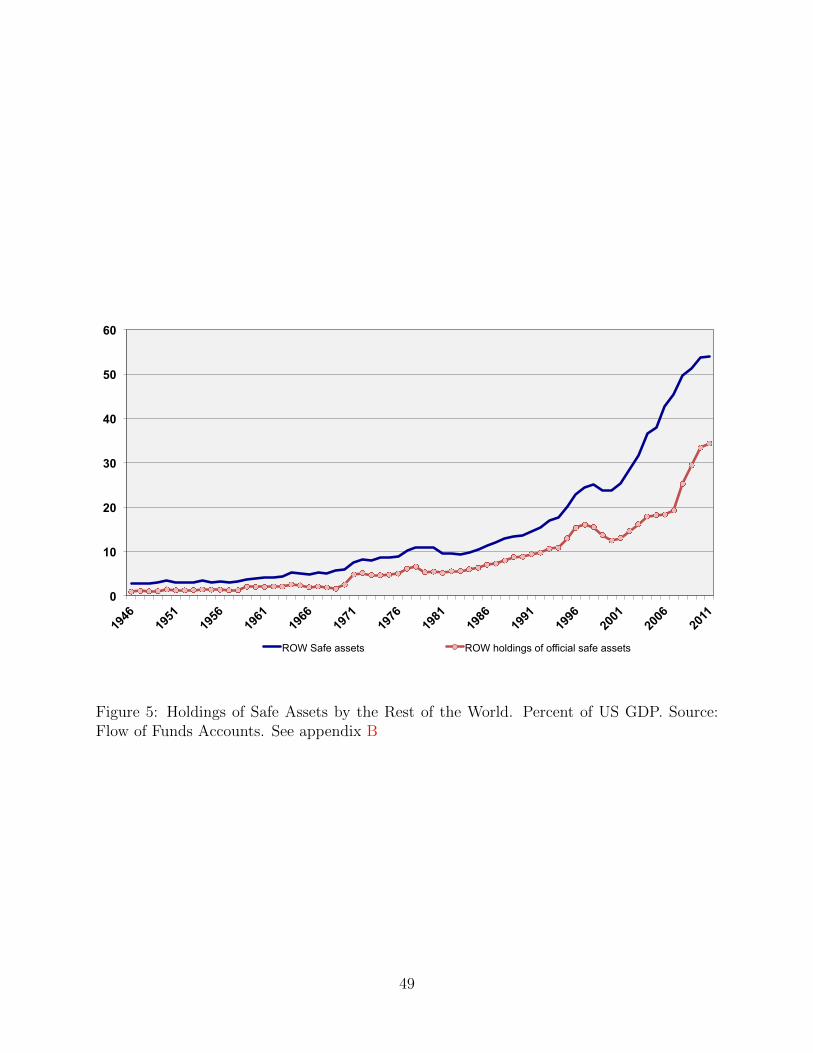
0

10

20

30

40

50

60

percent Holdings of US Safe Assets by the Rest of the World as % of US GDP

ROW Safe assets ROW holdings of official safe assets

Figure 5: Holdings of Safe Assets by the Rest of the World. Percent of US GDP. Source:Flow of Funds Accounts. See appendix B

49

0

20

40

60

80

100

120

140

160

percent US Real Private Sector* - Holding of Safe Assets and Supply of Risky Assets from Financial Sector, as % of US GDP

demand of safe assets from financial sector supply of risky assets to financial sector

*Households and Non-Profit Organizations + Non-financial Corporations

Figure 6: US Real Private Sector: Holdings of Safe Assets from Financial Sector and Supplyof Risky Assets to Financial Sector. Percent of US GDP. Source: Flow of Funds Accounts.See appendix B

50

0

10

20

30

40

50

60

70

percent US Financial Sector* - Holdings of Government Safe Assets, as % of US GDP

*Financial Business, net of Monetary Authority

Figure 7: Holdings of Government Safe Assets by the US Financial Sector. Percent of USGDP. Source: Flow of Funds Accounts. See appendix B

51

0 0.1 0.2 0.3 0.4 0.5 0.6 0.7 0.8 0.9 10

0.1

0.2

0.3

0.4

0.5

0.6

0.7

0.8

0.9

1

Prob. of monetary backstop (alpha)

Pro

b. o

f def

ault

and

infla

tion

default

inflation

Figure 8: Variations of probability of default and inflation with probability of monetarybackstop

52

53

Comments on “Global Safe Assets”

Peter R. Fisher

Gourinchas and Jeanne have provided a disciplined analysis of the critical challenge faced by both investors and central bankers: how to think about the apparent paucity of safe assets in the world today. Their paper has helped sharpen by own thinking, which I will briefly describe before making a few suggestions of further areas the authors might want to consider. I would like to thank the BIS for the honor of inviting me and recognize my BlackRock colleagues Ewen Cameron Watt, Ed Fishwick and Terry Keeley whose thoughts in this area have been of great benefit to me (but who bear no responsibility for my lack of discipline).

Our collective thinking on the apparent paucity of safe assets, and the “demise” of the risk-free rate, is badly muddled. First, we all fall into the trap of giving too much attention to supply and not enough to demand. Second, we need to be narrow our focus and distinguish more carefully four concepts that have shaped our thinking in recent years, namely (a) measures of the time value of money, (b) references for value, (c) hedging of interest-rate risk, and (d) the base asset, or reserve asset, of the banking system. Third, in our analysis of “safe assets” we need to be much clearer about “safety from what?” – the different elements of risk that are always present in an asset. Fourth, much greater emphasis needs to be given to differences in investment horizon – both between different agents and across time.

Think more about changes in demand. Ten years ago, when I was responsible for the U.S. Treasury’s debt management, I gave a speech about the long-run fiscal outlook in which I tried to draw attention to the U.S. government’s unfunded retirement and health care commitments and to suggest that more attention be paid to the actuarial position of the federal government. (“Beyond Borrowing: Meeting the Government’s Financial Challenges in the 21st Century”, Nov. 14, 2002.) As gloomy as I was then, looking back ten years, I could not have imagined that over the next decade we would triple federal debt outstanding, the federal government would explicitly assume the liabilities of Fannie Mae and Freddie Mac as wards of the state, and we would see a vast expansion of unfunded federal health care liabilities through both the Medicare drug benefit and universal coverage in the recent health care reform and the result would be that yields on the ten-year U.S. Treasury security would fall from 4.05 percent at the time of my speech to well below 2 percent today.

Clearly, demand has changed even more than supply. As has been already discussed in earlier sessions, emerging market and particularly Asian central banks have chosen to accumulate much higher levels of foreign currency reserves both to stabilize their exchange rate with the U.S. dollar and to insure themselves against having to seek resources in future crises from international authorities. The just-extended operation twist by the Federal Reserve is another source of extraordinary demand, for longer-maturity Treasury securities. Of course, other sources of changes in the behavior of demand can be attributed to higher household and corporate savings, weaker expected growth and a lower expected path of short-term rates, and safe-haven demand because of the European debt crisis.

So while supply of safe assets is easier to measure we must be careful not to let that distract us form what is more important if more elusive: the variability of demand.

Let me note here that while central banks may not feel bounded by the constraint of zero interest rates, in important ways investors are constrained by the zero interest rate boundary, a point I will return to.

54

What are we talking about? When we talk about safe assets, or the risk-free rate, there are several different subjects that we often conflate.

First, we need to have a measure of the time value of money. We need a discount rate to apply to future cash flows to bring them into present values and we can use sovereign bond curves, interest rate swap curves or corporate credit yield curves to do this.

Second, we need a reference for value. In market practice, we think of the benchmark from which we measure credit spreads – which could be sovereign bonds or corporate bonds. Let me note that in the 1960s and 1970s, when we spoke of the “benchmark” in the U.S. market we were most likely to be talking about either bonds of General Motors or American Telephone & Telegraph which were thought of as the appropriate “reference for value” in assessing spread relationships. But in discussing references for value we can also be thinking (with much more formality and rigor) about the capital asset pricing model and the use of a risk-free rate to help construct portfolio preferences.

Third, there is a related but distinct concept of the hedging-vehicle of choice – meaning the asset or instrument that investors turn to when they seek to hedge away certain risks, most tellingly interest rate risk. Indeed, the switch from thinking about corporate bonds as the benchmark to the ten-year U.S. Treasury security occurred as investors came to think about how best to hedge interest rate risks, particularly the duration risks associated with mortgage-backed securities.

Fourth, there is the concept of the base asset or reserve asset in any banking system, on which banks build their balance sheets. One can think of this simply as a low volatility asset, or low credit risk asset, around which investors or bank balance sheet managers diversify into riskier assets. Or one can think of this as the base asset in the sense of being the starting point for the money multiplier. While some prefer to think of only central bank liabilities as playing the role of “high-powered money” and, thus, the beginning of the money multiplier, it does appear that sovereign bonds in general, and U.S. Treasury securities in particular, also play an effective role as the base asset in the banking system.

Part of the cause of our muddled thinking about this subject is a consequence of the fact that, over the last few decades, sovereign bonds have happened to be pretty good at playing each of these four roles. The sovereign yield curve provides a measure of the time value of money. The capital asset pricing model provided a context for us to use sovereign bonds and, particularly, U.S. Treasuries, as a proxy for the theoretical risk-free rate in pricing other assets. As we experienced significant interest rate volatility in the 1980s and1990s, sovereign bonds played as useful role as a hedging vehicle for interest rate risks. And finally, sovereign bonds have increasingly been recognized as the base asset on bank balance sheets – and central bank balance sheets.

(As a personal note, in the early 1990s when I worked at the Federal Reserve Bank of New York, I recall fondly the stern lectures that I received from my counterparts at the Bundesbank about how embarrassed I should be because a real central bank would not monetize the profligacy of its Treasury – the way that the Federal Reserve did. What I recall fondly is the fact that I never received a satisfactory explanation of why we should be embarrassed to finance the profligacy of our Treasury in light of the Bundesbank’s readily-apparent willingness to finance the profligacy of our Treasury.)

In a gold regime, however, while gold can play the role of the banking system’s base asset, gold cannot and did not provide us with a measure of the time value of money. We might debate whether gold can play the role of a reference for value although I would suggest that because of it’s lack of intrinsic value it can play the role of unit of account precisely because of it’s lack of intrinsic value it cannot help us value other assets in constructing a portfolio.

Safe from what? In discussing the apparent paucity of safe assets we need greater attention to all the different elements of risks that investors and bankers are seeking safety from.

55

The concept of a risk-free rate, or risk-free asset, helps frame our thoughts about valuing assets but ultimately it leads us astray. There is no such thing as a risk-free asset, never was and never will be. There are assets with that carry less of certain risks than other assets and than other risks. While sovereign bonds in general, and U.S. Treasuries in particular, have been thought of as having high credit quality and as being highly liquid and, thus as having negligible credit and liquidity risks, for much of the last few decades we have been entirely accustomed to high levels of interest rate and currency volatility and, thus, mark-to-market risks in the value of bonds. Nominal bonds, of course, carry the risk of a loss of real value because of inflation. However, if you are worried more about deflation then sovereign bonds are a particularly attractive investment. And so on.

Frankly, the apparent paucity of safe assets is not the issue. The issue is the apparent paucity of high quality, liquid assets with the returns from the term structure that both public and private investors have come to expect.

Risk is deviation from objective. So depending on our objectives we value risks in different ways and are comfortable with some and not others.

The importance of horizon. Investment horizon is a tremendously important and less analyzed piece of the puzzle. Financial euphoria can be thought of a condition in which investors have indefinitely long investment horizons and, thus, systematically under value liquidity. Financial crisis can be thought of as the condition when investors have extraordinarily short investment horizons and place an extremely high value on liquidity. This frames the portfolio construction process as choices relative “liquidity give up” – and the longer one’s investment horizon the more likely one is to think in terms liquidity foregone.

I mentioned that central banks might feel unconstrained by the zero-interest rate boundary. Unfortunately, because of our relatively short investment horizon most investors are forced to live in a nominal world and, as a consequence, we are constrained by the zero interest rate boundary. While investors can calculate real returns they cannot “eat” them in a given quarter’s performance. Longer horizons might be desirable. But it is a fact that investment horizons tend to be short and variable.

A few suggestions for the authors.

First, the issue of horizon is immensely important and complicated and deserves considerable further attention by Gourinchas and Jeanne – and all scholars interested in clear thinking about safe assets. For example, the liquidity of an asset can be thought of as a hedge against investment horizon.

Second, I do not find the concept to the “inherently safe asset” to be either useful or durable. Changes in the macroeconomic and financial environment will always be changing what it is that we worry about and, therefore, will create changes in the risks that we are aware of and focus on. Thus, I would suggest looking at many more elements of risk than just credit and liquidity. I would also suggest that the stability of the banking system requires that (ex ante) we need to anticipate the reality that (ex poste) we will recognize the mistakes that have been made in assessing what is and what is not a safe asset.

Third, the problem of moral hazard is not resolved by limiting the definition of safe asset to public assets – as the ongoing European debt crisis reminds us. This is something the authors should give further attention.

56

Comments on “Global safe assets”

Fabrizio Saccomanni1

General remarks

Before commenting on some aspects of the paper by Gourinchas and Jeanne, I would like to make some general remarks on the broad policy issue raised by the topic of this seminar of the conference. We have achieved a full globalization of financial markets, truly global as emerging markets have been included; we have witnessed the creation of a huge amount of financial wealth but we ended up having no global safe assets. Nowadays, we see that there is a constant erosion of creditworthiness of issuers of safe assets, both public and private, and this process has been accelerated by the declaration taken in the French–German meeting in Deauville, on October 2011, where the introduction of the Private Sector Involvement (PSI) in the European crisis management has generated a plenty of tension.

The history of the International Monetary System, since the end of WWII, can be interpreted as the endless search for safe assets, safe from the erosion of value and the debasement of the currency that can derive from the misguided actions of elected governments, parliaments and central banks.

Gold was initially considered the safest asset as it was nobody's liability, but then the relative shortage of gold led to the creation of the gold-dollar standard, where the safety of dollar-denominated assets was indirectly guaranteed by the link of the dollar to gold. When that link was severed, the world de facto delegated to financial markets the task of determining which assets are to be considered safe and which not.

The problem with this arrangement is that markets are fickle and they can oscillate between one extreme, where all assets are safe, even junk bonds, Greek bonds, or Depfa bonds, and the opposite extreme, where there are virtually no safe assets, except a happy few, where every investor would like to place his or her money, irrespective of the yield.

Then, modeling the demand and the supply of safe assets should consider that the safety of an asset is a matter of convention and cannot be delegated to rocket scientists. One can compute it as the probability of default, the credit risk and the market risk. However, an important role is played by perceptions which, by their very nature, bring into the picture a qualitative assessment of the credibility of the issuer. In other words whether the issuer – private or public – will be able to carry on what is implicit in the definition of safe asset – namely to do everything to maintain the creditworthiness of its liabilities.

The age of financial globalisation has brought us to the verge of this second extreme. The extraordinary growth of financial activity has far outstripped the growth of real economies, leading to the accumulation of financial assets that are largely the liabilities - i.e. the debts - of countries, banks, corporations. The markets are telling us now that this process has gone too far and that a “deleveraging” - i.e. a reduction of the indebtedness - is now required by all debtors, public and private.

1 Director General - Banca d’Italia

57

The world economy is, in other words, confronted with a “global Triffin dilemma” in which the excessive indebtedness of the issuers of financial assets is now affecting the value of the assets themselves; of all assets, not just of reserve currencies, as in the early Triffin dilemma.

But, how is it possible to carry out this huge process of deleveraging in an orderly manner and without further destabilizing the world economy?

The obvious answer is that it may take time and in any case a longer period of time than that financial markets, suddenly become aware of the unsustainability of the situation, seem willing to concede.

The Model

The authors propose a stylized model for the supply and the demand of safe assets. The model not only shows that a safe asset can be backed by the fiscal and the monetary policy, but also points out that fiscal and monetary interventions are crucial in order to make the government debt a true safe asset and, as a consequence, “tying one’s hands” is sub-optimal. In this sense both fiscal and monetary instruments should be seen as viable policy instruments for stabilizing the price of government securities.

A crucial role is delegated to the real interest rate which acts as a stabilizing mechanism by clearing the safe asset market; as a consequence there should be no shortage of safe assets. At the same time monetary policy can act in fostering solvency of public debt and backstop a safe asset.

The core assumption of the paper is that the process of deleveraging can be assisted by policy actions by increasing the supply of safe assets. Hence the model embeds an optimistic view of the current situation: as the real interest rate is a stabilizing mechanism, in equilibrium there is no shortage of safe assets. All in all, the model projects a sense of complacency that contrasts with recent developments in the International Monetary System.

Based on IMF projections (GFSR, April 2012), by 2016 the supply of safe assets could decrease by $9 trillions due to the reduction in the number of sovereigns whose debt is considered safe. Moreover, the global demand for safe assets by the financial sector has steadily increased, and this sector represents the most relevant component of the total outstanding amount (the share of government securities worldwide held by the financial sector is greater than 50%; GFSR, April 2012).

Even if we accepted the possibility to use monetary policy to stabilize the price of government bonds, major problems may emerge in terms of implementation.

It is unclear to which extent monetary policy can act in fostering solvency of public debt and backstop a safe asset. For example, an unlimited monetary support of public debt would be unsustainable in the long run or a very conservative fiscal policy could become at some point politically unfeasible.

Assume the case of Japan (with a debt/GDP ratio around 230%) or even the US (with a debt/GDP ratio over 100%). Do you think that monetary policy, in case of a loss of confidence, could successfully intervene to safeguard the public debt of these countries? In order to examine the impact of monetary intervention to preserve safe assets one should use a model with multiple periods, in which the trade-offs between short-term and long-term effects are modeled and where policy-maker’s preferences with respect to inflation and insolvency are fully taken into account.

Finally, fiscal and monetary policies of individual countries, oriented to make their assets safe, are necessary but not sufficient conditions to cope with the growing divergence

58

between the demand and the supply of safe assets. A coordinated international approach is needed both at IMF and EU level, where the main source of tensions comes from. The authors seem to be confident that US Treasuries will continue to be the principal risk-free asset in the international market. Even if this is a strong conventional belief that will continue for some time, we should not rule out the possibility of a shift to a multipolar system. In this system there could be, potentially, an increase in the supply of a safe asset thanks to safe assets’ supplies originated in other reserve-currency centers. But at the same time the coexistence and the competition among these centers would require a high degree of international cooperation because in the short run, since volatility can increase as investors and intermediaries shift their investment from one currency to another.

International Monetary System

That is where the international dimension comes in. From a global perspective the scarcity of safe assets could lead to short-term volatility and runs on sovereign debt. As the US debt still represents the principal risk-free asset in the international markets, a possible shift from a dollar-based system to a multi-polar one could increase the supply of safe assets, alleviating exchange rate misalignments, large and persistent external imbalances and the accumulation of huge stocks of official reserves.

The leading idea of a multipolar system should be the setup of a strong multilateral surveillance, or perhaps even the creation of a multilateral reserve asset – as advocated by the President of the People’s Bank of China – which can be accepted by everybody.

The coexistence and the competition between two or more reserve currencies would probably require a high degree of international cooperation for ensuring the mutual consistency of national policies and containing the risk of instability due to the high degree of integration and interdependence of the International Monetary System. This calls for the G20 and the IMF to play an effective role in the governance of the International Monetary System.

The euro area

Let me consider the case of the euro area. Here the reforms introduced to deal with the crisis have increased the orientation of governments towards the adoption of programs of fiscal consolidation and debt reduction in a coordinated fashion through various procedural arrangements. However, as the ECB monetary policy must continue to be oriented towards the maintenance of price stability over the medium term, there is the need to enhance the crisis-management mechanisms. This could partially address the problems connected with the scarcity of safe assets. The search for safe assets is indeed indicated by the widening of spreads which reflects, on the one hand, the flight-to-quality process among European sovereign markets towards the German Bunds and, on the other hand, the lack of confidence towards highly indebted countries, which should carry on the policies they committed to. Lately, the spreads appear to incorporate also the risk of the break of the euro.

In these circumstances, the goal of policy makers should be to establish a link between the activity of the ECB and the new financial mechanisms that have been created to deal with this crisis; this link must be built and achieved and a cooperative approach should be adopted to deal with the legal and institutional problems that may arise. If we do not introduce this additional dimension it will be difficult to convince markets that the process of deleveraging and flight-to-quality will not lead to further source of instability and tensions.

59

However, as a final point let me say that monetary policy alone cannot be sufficient in stabilizing the asset prices of sovereign debts in Euro area. The crisis points to a failure in achieving a complete convergence and cooperation between national fiscal policies and national banking supervision practices. Although significant progress has been made in reinforcing euro-area governance, a change of pace is required.

If governments, the EU authorities, the ECB itself, judge the progress of the crisis-hit countries in fiscal consolidation and structural reform positively, this must be followed by a practical commitment on their part to orient the markets’ assessments in the same direction. The current yield spreads of government securities do not seem to take account of what has been accomplished and seem to reflect a risk of the demise of the euro, which all authorities are solemnly excluding. A strong measure of consistency between policy objectives and policy actions is required.