
BIOTIC AND ABIOTIC FACTORS AFFECTING THE SURVIVAL OF ...
69
BIOTIC AND ABIOTIC FACTORS AFFECTING THE SURVIVAL OF LISTERIA MONOCYTOGENES IN PRAIRIE POTHOLE SOILS AND SEDIMENTS A Thesis Submitted to the Graduate Faculty of the North Dakota State University of Agriculture and Applied Science By Nicholas Stephen Dusek In Partial Fulfillment of the Requirements for the Degree of MASTER OF SCIENCE Major Program: Genomics and Bioinformatics March 2017 Fargo, North Dakota
Transcript of BIOTIC AND ABIOTIC FACTORS AFFECTING THE SURVIVAL OF ...

BIOTIC AND ABIOTIC FACTORS AFFECTING THE SURVIVAL OF LISTERIA
MONOCYTOGENES IN PRAIRIE POTHOLE SOILS AND SEDIMENTS
A Thesis
Submitted to the Graduate Faculty
of the
North Dakota State University
of Agriculture and Applied Science
By
Nicholas Stephen Dusek
In Partial Fulfillment of the Requirements
for the Degree of
MASTER OF SCIENCE
Major Program:
Genomics and Bioinformatics
March 2017
Fargo, North Dakota

North Dakota State University
Graduate School
Title
Biotic and abiotic factors affecting the survival of Listeria monocytogenes
in prairie pothole soils and sediments
By
Nicholas Stephen Dusek
The Supervisory Committee certifies that this disquisition complies with North Dakota
State University’s regulations and meets the accepted standards for the degree of
MASTER OF SCIENCE
SUPERVISORY COMMITTEE:
Dr. Peter Bergholz
Chair
Dr. Phil McClean
Dr. Anne Denton
Approved:
04/11/17 Dr. Phil McClean
Date Department Chair

iii
ABSTRACT
The diversity-invasion relationship states that more diverse communities are more
resistant to invasion. Listeria monocytogenes – a gram-positive facultative anaerobe, soil
saprotroph, and opportunistic human pathogen – is capable of surviving in a diverse range of
habitats, including soil, and several recent studies have shown that the prevalence of L.
monocytogenes in soil increases with proximity to surface water. In addition, L. monocytogenes
resides frequently in the guts of ruminants and poultry, creating many opportunities for
deposition in soil. However, little work has been done to examine the effects of native soil
microbiota on the survival of the pathogen. This thesis builds on previous work by examining
microbial community diversity in the prairie pothole ecosystem and how it impacts the survival
of L. monocytogenes. Results indicate that survival of L. monocytogenes does not seem to differ
greatly as an effect of community diversity.

iv
ACKNOWLEDGEMENTS
I received help from a great many people in the completion of this thesis. Foremost
among these is my thesis advisor, Dr. Peter Bergholz, whose guidance and advice proved
invaluable throughout my studies and various research projects. The two other members of my
committee, Dr. Phil McClean and Dr. Anne Denton, were able to provide me with perspectives
on different areas of genomics and bioinformatics outside of microbiology, and thus helped
contribute to my breadth and depth of knowledge in the field.
I also received help from many people in the laboratory, including Kaycie Schmidt,
Austin Hewitt, and fellow graduate students Oleksandr Maistrenko, Chelsey Grassie, and
Morgan Petersen. Besides providing extra sets of hands, they made lab work enjoyable. I would
also like to thank the group at the USGS – Sheel Bansal, Jake Meier, and Alec Boyd – who
provided not only access to sampling areas, but help in collecting the samples for my thesis
project.
Additional thanks go to my funding sources, without which I would have had a hard time
doing any research: The National Science Foundation (NSF DEB, award no. 1453397) and the
National Institute of Food and Agriculture (NIFA-AFRI, award no. 2013-69003-21296).
Lastly, I would like to thank all those – faculty, staff, and fellow graduate students – in
NDSU’s Department of Microbiological Sciences, for creating an enjoyable environment in
which to conduct research.

v
TABLE OF CONTENTS
ABSTRACT ................................................................................................................................... iii
ACKNOWLEDGEMENTS ........................................................................................................... iv
LIST OF TABLES ........................................................................................................................ vii
LIST OF FIGURES ..................................................................................................................... viii
CHAPTER 1. LITERATURE REVIEW ........................................................................................ 1
The diversity-invasion relationship ............................................................................................. 1
Listeria monocytogenes ............................................................................................................... 4
The Prairie Pothole Region of North America ............................................................................ 7
CHAPTER 2. FACTORS IMPACTING SURVIVAL OF LISTERIA
MONOCYTOGENES IN PRAIRIE POTHOLE SOILS AND SEDIMENTS ............................ 10
Introduction ............................................................................................................................... 10
Materials and Methods .............................................................................................................. 13
Preparation of glucose defined minimal media for growth of Listeria monocytogenes ........ 13
Listeria monocytogenes strain used for soil microcosm study .............................................. 17
Growth of Listeria monocytogenes for inoculating soil microcosms .................................... 17
Soil sample collection............................................................................................................ 18
Sample processing ................................................................................................................. 20
Inoculation of soil microcosms with Listeria monocytogenes .............................................. 21
Measurement of Listeria monocytogenes death rate by plate count...................................... 22
Death curve analysis of Listeria monocytogenes count data ................................................. 22
Extraction of DNA from soils for microbiome sequencing .................................................. 23
16S microbiome sequencing using the V3-V4 Dual Indexing (DI) approach ...................... 25
Microbiome sequence analysis using QIIME ........................................................................ 25
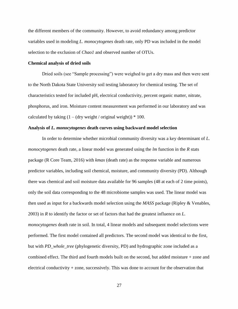
Chemical analysis of dried soils ............................................................................................ 27

vi
Analysis of L. monocytogenes death curves using backward model selection ..................... 27
Canonical Correspondence Analysis of Bacterial and Archaeal Families ............................ 28
Results ....................................................................................................................................... 30
Soil and sediment chemical attributes ................................................................................... 30
16S sequencing and taxonomic assignment .......................................................................... 32
Microbial community alpha diversity ................................................................................... 33
Factors with the greatest impact on L. monocytogenes death rate ........................................ 36
Patterns of microbial diversity in prairie wetlands with hydrography and land use ............. 39
Discussion ................................................................................................................................. 48
Microbial community diversity does not account for much variation in L.
monocytogenes death rate ...................................................................................................... 48
Wetlands are sources of methane while uplands are sources of carbon dioxide ................... 51
REFERENCES ............................................................................................................................. 53

vii
LIST OF TABLES
Table Page
1. Stock components in glucose-defined minimal media (for 50 mL) ......................................... 14
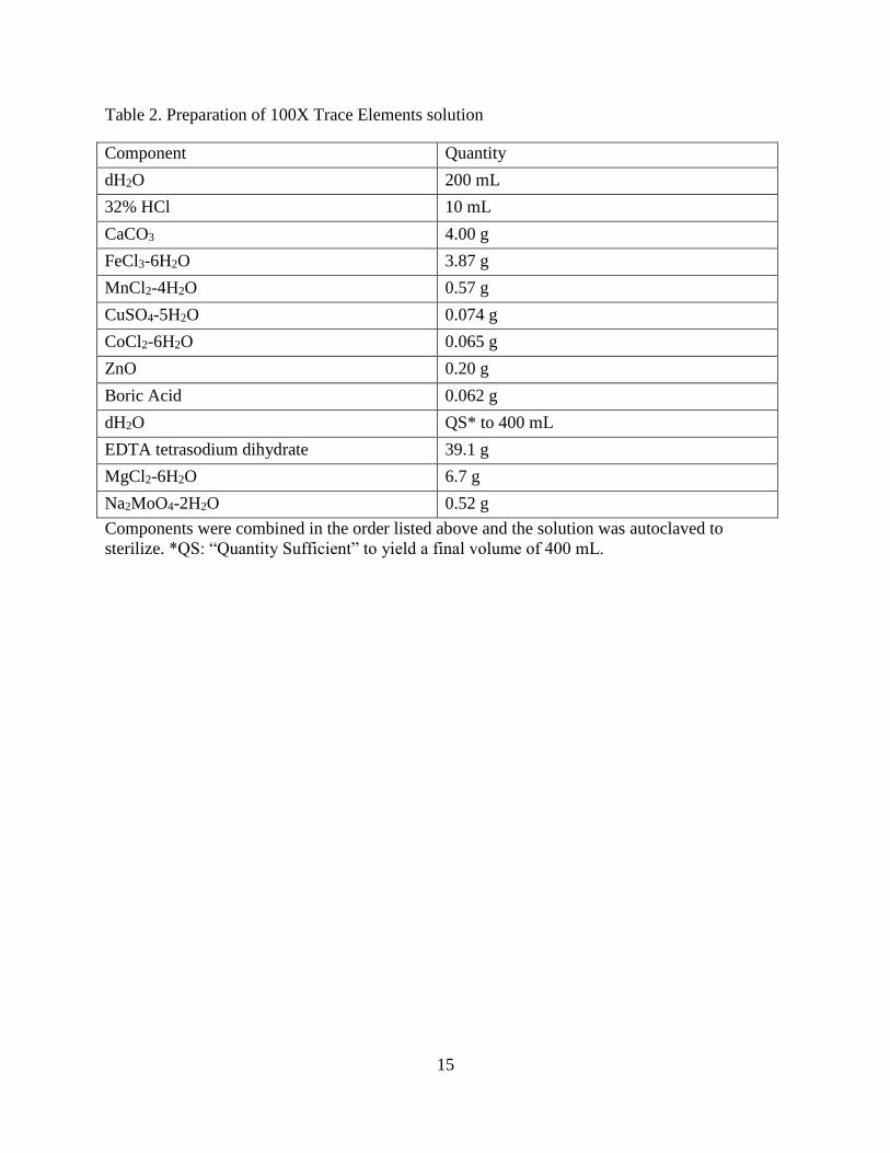
2. Preparation of 100X Trace Elements solution .......................................................................... 15
3. Preparation of 1000X Vitamins solution .................................................................................. 16
4. Preparation of 100X Amino Acids solution.............................................................................. 16
5. Listing of samples taken at each wetland. ................................................................................ 20
6. Extraction time points of each sample ...................................................................................... 24
7. Differences in prairie pothole chemistry by hydrography ........................................................ 31
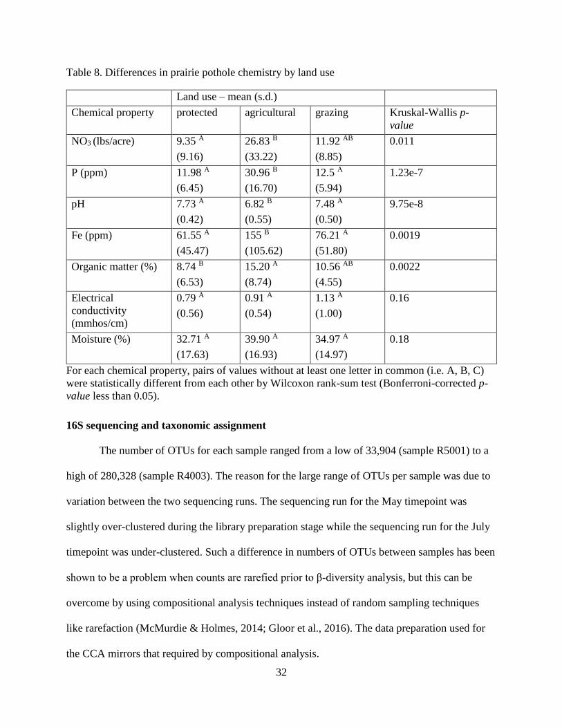
8. Differences in prairie pothole chemistry by land use ............................................................... 32
9. Differences in alpha-diversity by hydrography ........................................................................ 34
10. Differences in alpha-diversity by land use .............................................................................. 35
11. Predictor variables chosen by backwards model selection. .................................................... 38

viii
LIST OF FIGURES
Figure Page
1. Wetland sampling scheme. ....................................................................................................... 19
2. Percentage unassigned OTUs by taxonomic level.. .................................................................. 33
3. Difference in Faith’s Phylogenetic Diversity between hydrographic zones.. ........................... 35
4. Difference in Faith’s Phylogenetic Diversity between land use classes. .................................. 36
5. Death rate of L. monocytogenes by hydrography. .................................................................... 37
6. Death rate of L. monocytogenes by land use. ............................................................................ 38
7. CCA triplot with samples coded by hydrography..................................................................... 41
8. CCA triplot with samples coded by land use. ........................................................................... 42
9. Change in abundance of Acidobacteria with hydrography....................................................... 44
10. Change in abundance of Actinobacteria with hydrography. .................................................. 45
11. Change in abundance of Chloroflexi with hydrography. ........................................................ 46
12. Change in abundance of Euryarchaeota with hydrography. .................................................. 47
13. Change in abundance of Proteobacteria with hydrography. .................................................. 48

1
CHAPTER 1. LITERATURE REVIEW
The diversity-invasion relationship
The diversity-invasion relationship, first described by Charles Elton over 50 years ago,
was the name given to the observation that more diverse communities tend to be better at
resisting colonization by invasive species (Elton, 1958). The leading explanation for this
phenomenon is that more diverse communities are more efficient at exploiting resources, leaving
less niche space for invaders to colonize (Falcao Salles et al., 2015; Tilman, 2004). A study by
van Elsas and colleagues demonstrated a diversity-invasion relationship between Escherichia
coli and soil microbial communities of varying diversity (van Elsas et al., 2012); community
diversity was manipulated by serially diluting native soils in autoclaved soils, resulting in
successively diminished native microbiota. E. coli inoculated into less diluted (more diverse)
soils died faster than in less diverse treatments.
Another study conducted by Salles and colleagues looked specifically at the effect of
resource pulses on the ability of communities to resist invasion (Falcao Salles et al., 2015). If
efficiency of resource exploitation is the key driver of the diversity-invasion relationship, then
resource pulses, even in very diverse communities, should free up extra niche space for invaders.
In their study, Salles et al. found that E. coli survival was negatively correlated with community
species richness. But upon the introduction of a resource pulse (D-Galactose), even in the most
diverse treatment where E. coli had declined in density to nearly undetectable levels, the
increased resources strongly favored the proliferation of the pathogen. In the 5-, 15-, and 30-
species communities where D-Galactose was added, E. coli abundance rebounded to 104-105
CFU/mL. The same uptick was not observed in the control communities. This result provides

2
support for the hypothesis that resource availability is what drives the diversity-invasion
relationship.
From the two studies mentioned above, it would appear that E. coli, when treated as an
invasive species in soil, exhibits a diversity-invasion relationship. However, community diversity
is only one possible factor among several thought to affect invasion success. As with many
different areas of ecology, more work has been done in studying the invasion ecology of animals
and plants than has been done studying microbes. But in regards to invasive plant species, key
factors influencing invasion success include wide dispersal over short and long distances,
frequency and density of invasion events (propagule pressure), a generalist physiology that
allows for adaptation to many different environments, and the ability to grow quickly and
outcompete native flora (Dukes & Theoharides, 2007). Native community diversity, then, may
not be the most important factor, or even a significant factor, in every invader-ecosystem
relationship.
A 2015 study by Hambright and colleagues focused on the organism Prymnesium
parvum, a marine alga that has demonstrated the ability to invade freshwater lakes and cause
harmful algal blooms (Hambright et al., 2015; Hambright 2012). Researchers in this study started
with natural freshwater microbial communities and altered the amounts of resources that each
microcosm received. In addition to monitoring community diversity and resource availability,
Hambright and colleagues also looked at the effects of propagule pressure on the success of
invasion. In contrast to the two E. coli studies mentioned previously, community diversity and
resource availability were not found to have impacted P. parvum invasion success. Rather, only
propagule pressure influenced whether or not the invasion succeeded, with higher and more
frequent propagules establishing the organism more successfully.
3
Disagreements among the current body of research in invasion ecology suggest several
possibilities with regards to the diversity-invasion relationship. Perhaps the simplest explanation
for these contradictions is that microcosm studies, although informative, do not closely enough
resemble the natural communities and invasion events they are being used to model. This is
especially true of microbial assemblages – microcosms created by inoculating sterile soil with a
mixture of several pure cultures – where microbial community members are limited only to those
which can be cultured in the laboratory. But even in microcosms created from soil samples that
have not been manipulated, it may not be feasible to simulate the myriad environmental
conditions that occur in natural ecosystems, such as precipitation events, temperature
fluctuations (both within and between days and seasons), and different chemical resources that
could be entering the system.
Another possible explanation could be that the organisms being used as model invaders
are not invasive species with respect to the ecosystem under study. For example, pathogenic
strains of E. coli may prefer the mammalian gut as a native habitat, and therefore could be
considered an invasive species if deposited in extrahost environments such as soil, but there are
several groups of environmental E. coli that may do quite well in soil. Some have even claimed
that certain E. coli phylotypes can persist in soil long-term, possibly with growth (Brennan et al.,
2016). A third, and more complex explanation for the disagreement between such studies is that
some invasive species are not sensitive to community diversity while others are, the implication
being that the diversity-invasion relationship is not a universal phenomenon, but instead depends
on the specific invader-community combination (D’Antonio & Levine, 1999). This may be
especially true if resource exploitation is not the dominant factor governing invasion success. For
4
example, resource availability may not matter much if the invader can free up resources by
selectively killing other closely-related organisms that compete for the same type of resources.
It seems then that some evidence has mounted in support of the diversity-invasion
relationship, but it may not be generalizable to all invaders or native communities. If this is the
case, then it would be necessary to examine each invasive organism’s particular sensitivity to
native community diversity in order to determine how best to prevent invasion.
Listeria monocytogenes
Listeria monocytogenes is a gram-positive facultative anaerobe, an opportunistic human
and animal pathogen, and the causative agent of Listeriosis (Cossart, 2011). L. monocytogenes
rarely causes illness in healthy individuals, but is particularly dangerous for
immunocompromised populations and pregnant women, with a mortality rate between 20 and
30% (Cossart, 2011). The main route of transmission of L. monocytogenes in humans is through
the food supply due to the ability of the pathogen to survive on food processing equipment (Cerf
& Carpentier, 2011), in food (especially poultry and livestock, Wiedmann et al., 2004; Caugant
et al., 2003), and in soils (Piveteau et al, 2013; Wiedmann et al, 2006). The success of L.
monocytogenes in food processing environments has been linked to its ability to survive (and
even grow) at low temperatures and form biofilms that are difficult to remove (Ahmed et al,
2015; Kathariou et al, 2006; Banks et al, 1990). However, the factors affecting L. monocytogenes
survival in soil are not as clearly understood, due in part to the complexity and heterogeneity of
soil environments.
Many studies have been conducted to assess the prevalence of L. monocytogenes and its
ability to survive in soil. One of the earliest of these studies was conducted by Welshimer in
1960, where L. monocytogenes was inoculated into microcosms containing two different types of

5
autoclaved soil – “fertile” and “clay” – and cell density was monitored by plate counts at regular
intervals (Welshimer, 1960). Provided with adequate moisture, L. monocytogenes was still
detectable at 295 days in both soil types, indicating that soil can act as a suitable habitat for the
organism. A more recent study by Hartmann and colleagues on a sample set of 100 French soils
looked at a wider range of soil physical, chemical, and biotic factors in affecting the survival of
L. monocytogenes (Hartmann et al., 2013). They found soil chemistry – specifically the
saturation rates of various cations – to have the largest impact on L. monocytogenes survival, and
that in autoclaved soils, L. monocytogenes was detectable through the end of the 84-day study. In
a subset of 9 of the soils, they examined the effect of the soil microbiota on the survival of L.
monocytogenes by inoculating an autoclaved and non-autoclaved microcosm for each soil.
Interestingly, survival was reduced by the native microbiota, but only in those soils with a pH
above 7. Below a pH of 7, no difference in survival was observed between autoclaved and non-
autoclaved soils. However, L. monocytogenes survival, on the whole, was worse below pH 7
than it was in either treatment above pH 7. This suggests that L. monocytogenes survival may be
governed by complex interactions between biotic and abiotic factors.
Microcosm studies have been valuable in teasing apart factors that influence L.
monocytogenes survival when inoculated into soil, but they cannot provide the entire picture. For
one, inoculum levels for these experiments are often 106 to 108 cells – likely a much higher cell
density than would occur naturally through dispersal and deposition by animals. Therefore, some
researchers have chosen to model L. monocytogenes survival by examining its prevalence at the
landscape scale. One such study was conducted by Bergholz and colleagues where surface water,
soil, and soil surface drag swab samples were collected on and near fresh produce farms in New
York State and were tested for the presence of several different pathogens – including L.
6
monocytogenes – through enrichment-based isolation techniques (Bergholz et al., 2013). The
GPS location of each sample was recorded and prevalence data was mapped spatially along with
soil and water chemical data and weather data. These data were then used to create a
classification tree model identifying the factors with the greatest impact in predicting the
prevalence of L. monocytogenes. Results indicated a base prevalence of 15% for L.
monocytogenes among all samples, and the terminal rules in the classification tree indicated local
prevalence of up to 45-50%. In this case, available water storage and proximity to both surface
water and grazing pastures were the most informative factors in predicting the likelihood of L.
monocytogenes detection. A follow-up study (Strawn et al., 2016) validated the findings through
repeated drag swab field sampling and found that the proximity-based rules (proximity to surface
water and grazing pastures) were indeed able to predict the occurrence of L. monocytogenes with
reasonable accuracy.
Many more studies on the survival and prevalence of L. monocytogenes have been
conducted than can be discussed here, but the common theme is that factors relating to the
availability of moisture – whether it be proximity to water sources or soil physical characteristics
that affect the storage of moisture – have the greatest impact on L. monocytogenes survival.
Although some brief examinations on the impact of the native microbiota on L. monocytogenes
survival have revealed a potential role for the soil microbiome (Hartmann et al., 2013, Vivant et
al., 2013), more detailed approaches are needed to characterize the interactions between L.
monocytogenes and the soil microbiome with a focus on the diversity-invasion relationship.
Furthermore, although L. monocytogenes prevalence increases with proximity to surface water,
little has been done to investigate the plausibility of different freshwater sources as potential
reservoirs for L. monocytogenes persistence and growth. Several studies have shown that L.

7
monocytogenes can be isolated from surface water and sediments in small creeks and lakes
(Topp et al., 2007; Bergholz et al., 2013) and one study goes so far as to suggest that various
Listeria species – including L. monocytogenes – are capable of permanently colonizing
freshwater sediments (Scherer et al., 2016). Therefore, more work needs to be done to 1)
determine the role of the microbiome in the ability of L. monocytogenes to survive in soils once
deposited and 2) elucidate the role that surface water plays in providing a suitable niche for L.
monocytogenes, both in freshwater sediments and surface water proximal zones.
The Prairie Pothole Region of North America
The Prairie Pothole Region of North America covers approximately 900,000 km2 across
Saskatchewan, Alberta, and Manitoba in Canada and North Dakota, South Dakota, Minnesota,
and Iowa in the United States (Harju, et al., 2005). The region is so named for the thousands of
microlakes – prairie potholes – left by glacial depressions about 12,000 years ago, and serves as
the breeding grounds for a majority of the continent’s waterfowl, earning it the nickname
“America’s Duck Factory” (Gleason et al., 2013). Because of their near ubiquity in the
aforementioned regions of Canada and the United States, prairie potholes can be found
embedded in a variety of different ecosystems, including forests, grasslands, grazing pastures,
and agricultural fields. Furthermore, due to their small size and isolation from other bodies of
water, they are sources of surface water which may act as reservoirs for foodborne pathogens.
As was mentioned in the previous section, the prevalence of L. monocytogenes has been
shown to increase with proximity to both surface water and grazing pastures (Bergholz et al.,
2013; Strawn et al., 2016). This is especially important for areas that irrigate crops using ground
or surface water that could potentially be harboring foodborne pathogens. One such area is the
Salinas river valley in California, a major production region for leafy greens. In a 2-year study by

8
Cooley and colleagues looking at lakes and rivers near farm fields in the Salinas River Valley,
the average prevalence across all samples collected was 65% for Salmonella and 43% for
Listeria (Cooley et al., 2014). A similar potential may exist for prairie potholes to harbor L.
monocytogenes and other foodborne pathogens. But the question of whether or not L.
monocytogenes can persist in and even permanently colonize wetland sediments remains to be
seen, and may depend on a mosaic of biotic and abiotic factors and their combined effects. Since
the prairie pothole region serves as the breeding ground for migratory waterfowl, evidence
showing the ability of foodborne pathogens such as L. monocytogenes to survive in wetland
sediments could have important implications for controlling the spread of these pathogens in
produce fields.
Aside from their potential role as reservoirs for foodborne pathogens, prairie pothole
wetlands are also believed to play a critical role in the global carbon cycle, including production
and/or sequestration of the greenhouse gases carbon dioxide, methane, and nitrous oxide
(Gleason et al., 2013; Gleason et al., 2015). However, the conditions under which these wetlands
may act as either carbon sources or carbon sinks remain poorly understood. Studies in similar
ecosystems have revealed that small lakes and estuaries have a high potential for methane and
nitrous oxide emission, and that the rate of production of these gases is driven by a combination
of factors, including temperature, vegetation, and allocthonous inputs from agricultural and
grazing activities (Gleason et al., 2015; Jeppesen et al., 2015; Mitsch and Bernal, 2013).
Jeppesen and colleagues, in a long-term freshwater mesocosm study, found that temperature
alone did not account for significant differences in greenhouse gas fluxes (Jeppesen et al., 2015).
They found instead that the amount of available nutrients had a much more significant impact,
with annual CO2 and CH4 fluxes increasing in the low nutrient treatments and N2O fluxes

9
displaying the opposite trend. They attributed this effect to differences in the abundances of
macrophytes and phytoplankton in each system.
Another study by Gleason and colleagues examined the effect of wetland drainage and
restoration on CH4 and N2O fluxes (Gleason et al., 2015). Their results indicated 1) that the
wetlands themselves act as sources of CH4 whereas the associated upland soils have the potential
to act as CH4 sinks; and 2) that draining wetlands – a common practice in cropped fields –
reduces carbon sequestration potential, and that this reduction in sequestration potential may
persist even long after the wetlands have been restored.
These and other studies to date have placed emphasis on characterizing the water and
sediment chemistry across different land classifications, but little work has been done to link gas
flux measurements to the microbes driving the corresponding biogeochemical processes. By
studying greenhouse gas fluxes in association with microbial community structure, new insights
might emerge as to how changes in microbial community structure affect flux rates. It is likely
that changes in land use, nutrient input, temperature, and the like, alter the microbial
communities in these sediments, which in turn alter the production potential of the ecosystem.
Therefore, the microbes driving biogeochemical processes in prairie pothole sediments could be
a missing link in the relationship between spatio-chemical variation and greenhouse gas flux.

10
CHAPTER 2. FACTORS IMPACTING SURVIVAL OF LISTERIA MONOCYTOGENES
IN PRAIRIE POTHOLE SOILS AND SEDIMENTS
Introduction
The diversity-invasion relationship hypothesis attempts to explain the tendency of more
diverse communities to be better resisters of colonization by invasive species (Elton, 1958).
Some have suggested that this phenomenon is driven by resource partitioning effects in that more
diverse communities partition resources more effectively, leaving little left over for invaders to
exploit (Falcao Salles et al., 2015; Tilman, 2004). Soil microcosm studies with E. coli have
succeeded in reproducing this effect in the laboratory (van Elsas et al., 2012; Falcao Salles et al.,
2015), but the diversity-invasion relationship is not necessarily a universal phenomenon among
microorganisms. In a study of Prymnesium parvum (Hambright et al., 2015) – a marine alga
known to cause harmful algal blooms (Hambright 2012) – propagule pressure was the key
determinant in the establishment of a successful invasion. The diversity of the invaded
community did not play a role. Conflicting findings such as these raise questions as to whether
the diversity-invasion relationship is a universal phenomenon, or dependent on the particular
combination of invader and community. At present, more data is needed from a wider range of
organisms to determine whether or not the diversity-invasion relationship is a useful framework
in the study of microbial invasion ecology.
Listeria monocytogenes is a gram-positive facultative anaerobe, a food-borne pathogen,
and the causative agent of Listeriosis in humans and livestock (Cossart, 2011). The success of L.
monocytogenes as a food-borne pathogen is owed in part to its ability to form biofilms (Ahmed
et al, 2015; Kathariou et al, 2006; Banks et al, 1990), increasing the organism’s survival on food
processing equipment (Cerf & Carpentier, 2011). However, the pathogen also has many
11
opportunities to enter the soil and potentially become established there. The pathogen frequently
resides in the guts of various ruminants as well as poultry, and can be shed into the environment
(Piveteau et al., 2013; Wiedmann et al., 2004). Consequently, the use of manure from animals
harboring and shedding L. monocytogenes could result in direct introduction into farm fields. In
addition to residing in the guts of different species of livestock, L. monocytogenes can also act as
a soil saprophyte, thriving in environments with dead and decaying vegetation (Freitag et al.,
2009). Therefore, L. monocytogenes can be readily deposited into the environment and is capable
of – to some extent – surviving in soil (Vivant et al, 2013; Wiedmann et al, 2006), allowing for a
route of transmission to humans through fresh produce. Understanding the dynamic between L.
monocytogenes and the native microbiota in various soils – specifically, whether the diversity-
invasion relationship is an important factor in the survival and establishment of L.
monocytogenes in soil – may aid in identifying areas that are potential hotspots of pathogen
abundance.
One such area of importance to agricultural land management is the Prairie Pothole
Region of North America. Consisting of almost one million square kilometers of ponds and
microlakes spread across Southern Canada and the Midwestern United States (Harju, et al.,
2005), the Prairie Pothole Region provides breeding grounds for most of the continent’s
waterfowl (Gleason et al., 2013) and are thought to play a critical role in the cycling of
greenhouse gases. But determining their contribution to global greenhouse gas fluxes is not clear
cut; they have been shown to be sequesters of atmospheric carbon in some cases and emitters of
atmospheric carbon in others (Gleason et al., 2013; Gleason et al., 2015), and although
sequestration of atmospheric carbon reduces global CO2, it can come at the expense of increased
production of other greenhouse gases such as N2O and CH4 (Gleason et al., 2009). Moreover,
12
disturbances to prairie potholes, especially eutrophication, may increase the flux of one or more
of these greenhouse gases (Jeppesen et al., 2015; Mitsch & Bernal, 2013; Gleason et al., 2015).
Given the size of the prairie pothole region and the number of wetlands contained within it,
prairie potholes have the potential to be a major factor in the global greenhouse gas budget.
However, studies to date have focused mostly on variation in vegetation, temperature, and
chemical inputs to the wetlands. Comparatively little work has been done to study the microbial
communities in these ecosystems.
In addition to their role as contributors to the global greenhouse gas cycle, prairie pothole
may be important components in the transmission cycle of L. monocytogenes and other
foodborne pathogens due to their abundance in and around farm fields and their role as breeding
grounds for migratory waterfowl. Being that L. monocytogenes is commonly found in poultry, a
further look into the suitability of migratory waterfowl as a dispersal vector for the pathogen may
be warranted. Furthermore, several studies have shown that L. monocytogenes prevalence is
higher near streams and other sources of surface water, and that agricultural areas near these
water sources may be impacted (Bergholz et al., 2013; Strawn et al., 2016; Topp et al., 2007).
However, prairie potholes, as a result of their hydrographic isolation, vary dramatically with
respect to water chemistry, especially salinity (Sloan, 1972). As a result, it is unclear whether the
success of L. monocytogenes in riverine and lacustrine environments can be extended to prairie
potholes. More research is needed to determine under what conditions prairie potholes may act
as reservoirs for foodborne pathogens in general and what impact (if any) the native microbial
communities have on their survival.
In order to examine the role that microbial community diversity plays in affecting the
survival of L. monocytogenes as well as characterize the microbial communities in the prairie

13
pothole region and their impacts on greenhouse gas fluxes, two experiments were conducted in
parallel. The first was a microcosm experiment in which L. monocytogenes was inoculated into
prairie pothole soils and sediments from different land use types (agricultural, grazing, and
natural) and the death rates for each sample calculated. The second experiment was a
microbiome study examining the community structure and diversity in each of the different
sample locations. These data were then combined in order to determine if microbial community
diversity was a key driver of L. monocytogenes death rate. In addition, Canonical
Correspondence Analysis was applied to the soil chemical and microbiome data to identify
microbial families associated with different land types and environmental parameters.
Materials and Methods
Preparation of glucose defined minimal media for growth of Listeria monocytogenes
L. monocytogenes for inoculation into soil microcosms was grown in a glucose defined
minimal media (Egli & Schneebeli, 2013) with several modifications. The minimal media was
mixed fresh on the day of inoculation from several concentrated stock solutions and individual
components. Table 1 below list the volumes of components required to make 50 mL of media.
Tables 2-4 describe the makeup of the trace elements, vitamins, and amino acids solutions
respectively.

14
Table 1. Stock components in glucose-defined minimal media (for 50 mL)
Component Volume (mL)
1.28M Na2HPO4 (50X) 1.000
0.482M KH2PO4 (100 X) 0.500
2.67M (NH4)2SO4 (50X) 1.000
0.629M MgSO4 (100X) 0.500
0.5M EDTA (100X) 0.500
1M MOPS buffer, pH 7 (10X) 5.000
Trace Elements (200X) 0.250
Vitamins (1000X) 0.100
82.5mM Cysteine (100X) 0.500
205mM Glutamine (50X) 1.000
67mM Methionine (100X) 0.500
Amino acids (100X) 0.500
100 g/L Glucose (67X) 0.750
Sterile dH2O 37.9
Components were combined in the order listed above. The glucose, amino acid, and vitamin
solutions were kept at 4°C for stability. Individual amino acids (Glutamine, Methionine, and
Cysteine) were stored dry and dissolved in water at the time of media preparation.
15
Table 2. Preparation of 100X Trace Elements solution
Component Quantity
dH2O 200 mL
32% HCl 10 mL
CaCO3 4.00 g
FeCl3-6H2O 3.87 g
MnCl2-4H2O 0.57 g
CuSO4-5H2O 0.074 g
CoCl2-6H2O 0.065 g
ZnO 0.20 g
Boric Acid 0.062 g
dH2O QS* to 400 mL
EDTA tetrasodium dihydrate 39.1 g
MgCl2-6H2O 6.7 g
Na2MoO4-2H2O 0.52 g
Components were combined in the order listed above and the solution was autoclaved to
sterilize. *QS: “Quantity Sufficient” to yield a final volume of 400 mL.

16
Table 3. Preparation of 1000X Vitamins solution
Component Quantity
dH2O 100 mL
Biotin 2.0 mg
Folic acid 2.0 mg
Pyridoxine 10.0 mg
Thiamine HCl 5.6 mg
Riboflavin 5.0 mg
Niacin 5.0 mg
Cobalamin 5.0 mg
Pantothenic acid D-Calcium 10.9 mg
4-aminobenzoic acid 5.0 mg
Lipoic acid 5.0 mg
Nicotinamide 5.0 mg
Components were combined in the order listed above, stirred at ~600 rpm with a magnetic stir
bar until dissolved, and sterile-filtered with a 0.22 µM filter.
Table 4. Preparation of 100X Amino Acids solution
Component Volume (mL)
dH2O 100 mL
Histidine 1.35 g
Tryptophan 1.00 g
Leucine 1.00 g
Isoleucine 1.00 g
Valine 1.00 g
Arginine 1.21 g
Components were combined in the order listed above, stirred at ~600 rpm with a magnetic stir
bar until dissolved, and sterile-filtered with a 0.22 µM filter.

17
Listeria monocytogenes strain used for soil microcosm study
The strain of L. monocytogenes used for inoculation into the soil microcosms was strain
J0161 transformed with the pNF8 plasmid (provided by Mike Doyle and Cathy Webb at UGA),
engineered with an erythromycin resistance gene for selection and constitutively-expressed
Green Fluorescent Protein (GFP) for screening (Fortineau et al., 2000; Ma et al., 2011). J0161 is
an isolate of lineage II, a group more frequently found in non-clinical samples. But isolates from
lineage II have also been the causes of several outbreaks. Strain J0161 was found to be the cause
of a multi-state disease outbreak in the year 2000, originating from poultry deli meat (Olsen et
al., 2005; Ma et al., 2011). As such, it is a relevant strain for this study because 1) it has been
shown to cause disease in humans and 2) the 2000 outbreak was traced back to poultry,
indicating that it could be a likely candidate for dispersal via migratory waterfowl residing in
prairie potholes.
Growth of Listeria monocytogenes for inoculating soil microcosms
To prepare inoculum for the soil microcosm study, a frozen stock of J0161 was removed
from -80°C, streaked for isolation onto Brain Heart Infusion (BHI) agar containing 40 µg/mL
Erythromycin and grown at 37°C for 48 hours. This strain had been previously transformed with
a plasmid bearing genes for erythromycin resistance and Green Fluorescent Protein (GFP).
Isolated colonies were screened for fluorescence using a blue LED transilluminator. Positive
colonies were used to inoculate 10 mL each of BHI broth containing 40 µg/mL erythromycin for
plasmid maintenance. Tubes were shaken at 215 rpm for 48 hours at 37°C. Following growth on
BHI, 100 µL of culture was transferred to 10 mL of glucose-defined minimal media +
erythromycin and grown on a shaker as before. From this growth, a final passage was performed
by taking 100 µL of culture and placing it into 10 mL fresh glucose-defined minimal media +

18
erythromycin. After 48 hours of growth on the shaker, the culture (now in a tertiary passage) was
considered ready for inoculation into soil microcosms.
Soil sample collection
Prairie pothole soils and sediments were collected from three different areas near
Jamestown, ND, representing natural, agriculturally impacted, and grazing impacted prairie
pothole wetlands. Potholes classified as natural (or protected) were located in the Cottonwood
Lake Study Area (CLSA), a Long Term Research area maintained by the United States
Geological Survey (USGS, 2012) focused on studying the prairie pothole ecosystem. Potholes
classified as agriculturally impacted and grazing impacted were located on private land, and
permission for sample collection was obtained in cooperation with the USGS. At each pothole,
eight gas flux monitoring stations are installed, five within the wetland and three at increasing
distances away from the wetland (Gleason et al., 2013).
Soil and sediment samples were collected adjacent to four different gas flux stations at
each of 12 different wetlands on two different dates. Table 5 shows the samples collected on
each of the two sampling dates, along with wetland designation, wetland ID, and gas flux station
where the sample was collected. Figure 1 shows the relative locations of the different stations
within a wetland that samples were collected at. For each sample number in Table 5, the letter
and first number in the sample ID designates the wetland ID and the last number designates the
gas flux station. Station 1 was in the submerged wetland zone, station 2 at the wetland margin,
station 3 at the toe slope of the basin, and station 4 at the shoulder slope. The toe and shoulder
slopes were 2-5m and 70-100m from the wetland margin, respectively (linear distance, not
elevation). All wetlands starting with “P” were natural/protected. Wetlands R2, R4, and R5 were
grazing-impacted while R8, B5, and B6 were agriculturally-impacted. For example, sample

19
P3003 was taken at protected wetland 3 at the wetland basin’s toe slope whereas sample R2001
was from submerged sediment in a grazing-impacted wetland. The below set of samples was
collected twice – once on May 16, 2016 and again on July 26, 2016.
Figure 1. Wetland sampling scheme.

20
Table 5. Listing of samples taken at each wetland.
Samples Wetland Designation
P1001-1004
Natural/Protected
P3001-3004
P4001-4004
P6001-6004
P7001-7004
P8001-8004
R2001-2004
Grazing impacted R4001-4004
R5001-5004
R8001-8004
Agriculturally impacted B5001-5004
B6001-6004
Samples were collected with sterile plastic scoops and placed in 8 oz. Whirl-Pak® bags.
Submerged sediments were first unearthed with a shovel and the sample was then taken from the
removed sediment. All samples were kept in a cooler to protect from sunlight until returned to
the laboratory for processing. Upon returning to the laboratory, the cooler was kept at room
temperature overnight until samples could be processed.
Sample processing
The morning following sampling (beginning less than 24 hours after the first sample was
taken), soils and sediments were each separated into three fractions. The first fraction consisted
of approximately 1.5 mL in each of two 2-mL cryovials which were labeled with the sample
number and immediately frozen at -80oC for DNA extraction at a later date. The second fraction
consisted of 40 mL of either soil or sediment placed in a 160-mL sterile container. These
containers served as microcosms for analysis of L. monocytogenes survival, and were moved to a
20oC incubator to equilibrate to temperature prior to inoculation the following day. The

21
remaining material for each sample was moved to brown paper bags, weighed to get a starting
mass, and moved to 55oC for drying. Drying served the dual purpose of obtaining a dry weight
for soil moisture calculations as well as preparing the soils for chemical analysis.
Inoculation of soil microcosms with Listeria monocytogenes
L. monocytogenes broth cultures (prepared as described previously in “Growth of Listeria
monocytogenes for inoculating soil microcosms”) were removed from the shaker at the 48-hour
mark and were transferred to 15-mL conical centrifuge tubes. Cultures were pelleted by
centrifugation at 4,500 rpm, 4oC for 8 minutes and then resuspended in 5 mL 1X PBS to wash
cells. The centrifugation was repeated and the pellet was once again suspended in 1X PBS, this
time 10 mL. Cells in PBS were transferred to a sterile 500 mL flask for dilution to the target cell
density.
From previous test growths, it was known that L. monocytogenes in this media and
growth conditions reached a density of 1.2 x 10⁸ CFU/mL after 48 hours in the final passage.
This cell density was used to calculate the volume of diluent needed to reach the target cell
density of 1.0 x 10⁷ CFU/mL. The two tubes of cells in 1X PBS (total 20 mL at a theoretical cell
density of 1.2 x 10⁸ CFU/mL) were added to the 500 mL flask and diluted to a total volume of
240 mL 1X PBS, yielding a theoretical concentration of 1.0 x 10⁷ CFU/mL.
The diluted cell suspension was used to inoculate the soil microcosms at a volume of 4
mL per 40-mL microcosm, yielding an expected microcosm cell density of 1.0 x 10⁶ cells per
mL of microcosm. The inoculum was carefully mixed into the soil for each microcosm and the
microcosms were weighed. This was done to determine what the density of each microcosm was,
since the soil texture and moisture content varied widely between samples. After this,
microcosms were incubated at 20oC.
22
Measurement of Listeria monocytogenes death rate by plate count
To enumerate surviving L. monocytogenes, microcosms were plated 5 times in the first
10 days post-inoculation and once every 5-7 days thereafter until L. monocytogenes counts
declined below the limit of detection of 1 colony per plate (< 200 CFU/mL soil). To plate out
microcosms at each time point, a 0.5 mL aliquot of the soil from each microcosm was transferred
to a 50-mL graduated centrifuge tube. The amount of microcosm weighed to obtain 0.5 mL was
determined by dividing the total mass of the microcosm (representing 40 mL of microcosm) by
80. Then, working in a Biological Safety Cabinet (BSC), 10 mL of 1X PBS (e.g. a 1:20 dilution)
was added to each tube and tubes were mixed by vortex for 20-30 seconds, then allowed to settle
for at least 10 minutes.
For each sample, 1 mL of supernatant was taken by pipette without disturbing the settled
soil and was moved to a fresh 1.5-mL microfuge tube. This suspension was then serially diluted
twice 1:10 in 1X PBS to create the dilution series. Each dilution was plated in triplicate on
CHROMagar® (CHROMagar Media – Paris, FR) at a volume of 100 µL per plate using a sterile
hockey-stick spreader to evenly distribute the inoculum across the surface of the agar. Agar was
prepared according to package instructions and supplemented with a final concentration of 40
µg/mL of Erythromycin. Plates were allowed to dry open in the hood and were then covered.
Plates were placed at 37oC and allowed to incubate for 5-7 days. At the end of the incubation,
colonies were counted using a blue LED transilluminator.
Death curve analysis of Listeria monocytogenes count data
Replicate plate counts of survivors were averaged, and Log10 CFU/mL was estimated.
When the time series study was complete, log-transformed plate count data was exported as a
comma separated file and imported in R, v3.3.0 (R Core Team, 2016). For each microcosm, the

23
log CFU/mL values were plotted as a function of time (days post-inoculation) and were fit to a
Geeraerd model using the R package nlsMicrobio (Delignette-Muller & Baty, 2013). The full
Geeraerd model is a negative logistic function with three phases: 1) a flat lag phase where cells
are dying at very low rates (the shoulder); 2) a region of increasing and then decreasing rates of
cell death, with the inflection point being equal to the maximum death rate (kmax); and 3) a tail
where the death rate levels off, indicating either that all cells have died or that they have reached
a stable state supportable by their environment. Three different variations of the Geeraerd model
were available: 1) a model containing all three parameters, 2) a model containing only the
shoulder and kmax parameters, and 3) a model containing only the tail and kmax parameters. All
three models were applied to each curve, but in most cases, only one of the models converged to
a solution. In cases where more than one model fit the data, the model with the lowest sum of
squared errors was chosen. The key piece of information derived from the Geeraerd model fitting
was the model kmax, or rate parameter, which is the maximum death rate.
Extraction of DNA from soils for microbiome sequencing
DNA was extracted from the soil and sediment aliquots that had been stored at -80oC.
Extractions were performed using a two stage purification consisting of the MoBio PowerSoil®
kit followed by the MoBio PowerClean® kit, both according to the kit instructions. Half of the
samples were purified from the May sampling time point and half from the July time point.
Samples for extraction from the first time point were chosen in a pseudorandom manner such
that an equal number of samples would be sequenced from each sample site and from each
hydrographic zone within sample sites. At the July time point, samples were chosen that were
not sequenced the first time to complete the set of one microbiome per sample. Table 6 shows

24
which samples were sequenced from the May time point and which samples were sequenced
from the July time point.
Table 6. Extraction time points of each sample
Sample Time point Sample Time point Sample Time point
P1001 May P7001 July R5001 July
P1002 July P7002 May R5002 May
P1003 July P7003 July R5003 July
P1004 May P7004 May R5004 May
P3001 July P8001 May R8001 May
P3002 May P8002 July R8002 July
P3003 July P8003 July R8003 July
P3004 May P8004 May R8004 May
P4001 May R2001 May B5001 May
P4002 July R2002 July B5002 July
P4003 May R2003 May B5003 May
P4004 July R2004 July B5004 July
P6001 May R4001 July B6001 July
P6002 July R4002 May B6002 May
P6003 May R4003 May B6003 July
P6004 July R4004 July B6004 May
DNA was extracted for half of the soil/sediment samples at the May time point and half at the
July time point.
25
16S microbiome sequencing using the V3-V4 Dual Indexing (DI) approach
At each of the two timepoints, DNA samples (24 per time point) were sent to the
University of Minnesota Genomics Center (UMGC) for 16S microbiome sequencing. The
UMGC uses a dual indexing approach (Beckman et al., 2016) based on the Earth Microbiome
Project (EMP) primer set (Gilbert et al., 2014) which targets variable regions 3 and 4 (V3-V4) of
the bacterial 16S rRNA gene, frequently used in microbial taxonomic studies such as this. For
each sequencing run, all 24 samples were multiplexed on a single Illumina MiSeq® lane using
300 bp paired-end sequencing.
Microbiome sequence analysis using QIIME
Sequence data was received from the UMGC already demultiplexed, with forward and
reverse reads contained in separate FASTQ files for each sample. Reads were first quality
trimmed using trimmomatic in paired-end mode (Usadel et al., 2014). Trimmed reads for which
both read pairs survived were used as input for QIIME v1.9 (Quantitative Insights Into Microbial
Ecology; Knight et al., 2010). Reads were first joined using the join_paired_ends.py script with a
maximum percent mismatch threshold of 10%. Joined reads were then assigned sample names
according to a mapping file using the script multiple_split_libaries_fastq.py which performs
more quality trimming and places all sequences (with sample identifiers) into a single FASTA
sequence file, seqs.fna.
Using the seqs.fna file as input, operational taxonomic units (OTUs) were assigned using
the script pick_open_reference_otus.py. As the name suggests, the OTU picking strategy used by
this script is an open reference strategy. In open reference OTU picking, sequences are first
matched against a database of identified sequences – in this case, the Greengenes database, v13.8
(Andersen et al., 2006) with a percent OTU identity cutoff of 97%. Sequences that do not match

26
anything in the database are then clustered de novo and these new sequences are matched again
to the database. In most instances, the taxonomy assigned to these second round OTUs is not as
specific as that assigned to closed reference database hits. The output resulting from this
operation is an OTU table containing OTU IDs and assigned taxonomy.
The final step in a basic QIIME analysis is the alpha- and beta-diversity analyses which
are accomplished with the core_diversity_analyses.py script using the OTU table from the
previous step as input. By default, QIIME calculates three different measures of alpha-diversity:
observed OTUs, Chao1 richness (Chao, 1984), and Faith’s Phylogenetic Diversity (PD, Faith,
1992). The three metrics measure diversity in very different ways. Faith’s PD is the most
informative of the three because it is calculated based on the sum of branch lengths in the
community-wide phylogenetic tree. The tree is generated by QIIME based on the OTU tables
using the program FastTree (Price, Dehal, & Arkin, 2009). In this way, it measures not just the
number of different species (the case with observed OTUs), but it measures the degree of
relatedness between the members present. Additionally, the phylogenetic tree from which Faith’s
PD is calculated is the basis of UniFrac distance, the community dissimilarity metric preferred
by the developers of QIIME. UniFrac represents the “Unique Fraction” of phylogenetic tree
branch lengths between two samples (Knight et al., 2009) and is used as the default measure of
distance for β-diversity in QIIME.
Faith’s PD stands in contrast to Chao1 richness, which is a calculation based on the ratio
of singleton to duplicate OTUs. As such, Chao1 richness performs better as a metric for
completeness of sequence coverage rather than it does as a metric for community diversity.
Taken together, the measures help to provide a complete picture of diversity encompassing
effectiveness of sequence coverage, total number of different members, and the relatedness of
27
the different members of the community. However, to avoid redundancy among predictor
variables used in modeling L. monocytogenes death rate, only PD was included in the model
selection to the exclusion of Chao1 and observed number of OTUs.
Chemical analysis of dried soils
Dried soils (see “Sample processing”) were weighed to get a dry mass and then were sent
to the North Dakota State University soil testing laboratory for chemical testing. The set of
characteristics tested for included pH, electrical conductivity, percent organic matter, nitrate,
phosphorus, and iron. Moisture content measurement was performed in our laboratory and was
calculated by taking (1 – (dry weight / original weight)) * 100.
Analysis of L. monocytogenes death curves using backward model selection
In order to determine whether microbial community diversity was a key determinant of L.
monocytogenes death rate, a linear model was generated using the lm function in the R stats
package (R Core Team, 2016) with kmax (death rate) as the response variable and numerous
predictor variables, including soil chemical, moisture, and community diversity (PD). Although
there was chemical and soil moisture data available for 96 samples (48 at each of 2 time points),
only the soil data corresponding to the 48 microbiome samples was used. The linear model was
then used as input for a backwards model selection using the MASS package (Ripley & Venables,
2003) in R to identify the factor or set of factors that had the greatest influence on L.
monocytogenes death rate in soil. In total, 4 linear models and subsequent model selections were
performed. The first model contained all predictors. The second model was identical to the first,
but with PD_whole_tree (phylogenetic diversity, PD) and hydrographic zone included as a
combined effect. The third and fourth models built on the second, but added moisture + zone and
electrical conductivity + zone, successively. This was done to account for the observation that

28
the wetland and upland zones represent two distinct ecosystems, leading to a great deal of
covariation among the predictors.
Canonical Correspondence Analysis of Bacterial and Archaeal Families
Canonical correspondence analysis (CCA) was used to identify trends in bacterial and
archaeal family abundance driven by site and environment. Briefly, CCA is an ordination
technique that aims to identify the environmental optima for each taxon in multivariate datasets
(ter Braak, 1986; Verdonschot & ter Braak, 1995). The required data inputs for this method are
tables containing environmental data by sampling site and taxonomic counts by sampling site,
and the method assumes that the data are normally distributed. As a result, prior to CCA, the data
must be transformed and standardized such that they conform to the assumption of normality,
which can be accomplished using a standardization function.
To prepare the inputs for CCA, the OTU table from the QIIME analysis mentioned above
(out_table_mc2_w_tax_no_pynast_failures.biom) was converted to tab delimited format using
the biom command line utility (Caporaso et al, 2012) and was loaded into R. Taxonomic
assignment data was parsed into separate columns yielding a single data frame with each
taxonomic level represented as a unique column. All fields for which taxonomy could not be
assigned were standardized as “Unassigned” for consistency and to allow for querying of
important summary statistics, such as percentage unassigned OTUs at each taxonomic level.
Environmental data were assembled next, which consisted of the results of the soil
chemical testing added to gas flux data for CO2, CH4, and N2O. Gas flux measurements were
collected by the USGS at all the same sample sites where soils were collected. The dates of
measurement varied, with some occurring on the same day as soil sampling and some occurring
several days before or after. The difference between the dates of soil sampling and gas flux

29
measurement never exceeded one week. For both CO2 and CH4, a single outlier was present
requiring removal of the associated sample. This brought the total number of observations to 46.
For the N2O data, two outliers were present, which if removed, would have decreased the total
number of observations to 44. Furthermore, these two observations were from the same land
cover type (Agricultural), so the N2O data was excluded for the CCA in order to minimize loss of
samples.
Soil and gas flux data (minus N2O) were merged into a single table and transformed for
analysis. Proportional data (percentages of organic matter and moisture) were square-root arcsin
transformed first, and then all data were transformed using the standardizing function as
implemented in the R package vegan (Dixon, 2003). The OTU data were aggregated by
taxonomic Family and transformed from absolute to relative by dividing the count for each OTU
by the total number of OTUs in the respective sample. Relative abundance data were Hellinger
(square root) transformed, again using the implementation in vegan, and all OTUs with a
maximum relative abundance less than 0.0025 post-transformation were removed. The two data
tables (environmental and taxonomy data) were used as the inputs for CCA using the cca method
in vegan. In order to reduce complexity of the resulting ordination plot, specific taxa were
highlighted corresponding to their reported ecological role (e.g. methanogens, sulfur reducers,
etc.) and sites were color coded by the two different available metrics: hydrographic zone and
land use type. Environmental variables were represented as vectors with direction and magnitude
corresponding to the taxa and sample sites that they most characterized.

30
Results
Soil and sediment chemical attributes
Kruskal-Wallis (Kruskal & Wallis, 1952) and pairwise Wilcoxon rank-sum tests
(Wilcoxon, 1945) revealed several significant differences between soil and sediment chemical
attributes, both across different hydrographic zones and across different land use classes (Tables
7 and 8, respectively). With respect to hydrography, NO3 was significantly different between
zones 2 and 4, and Fe, electrical conductivity, and moisture were all significantly higher in zones
1 and 2 compared with upland soils. Focusing on the different land use classes, the impact of
land management practices in agricultural areas becomes clear: NO3 was significantly higher and
organic matter significantly lower in agricultural soils and sediments as compared to natural
wetlands. Furthermore, P and Fe were higher in agricultural wetlands than in both grazed and
natural wetlands while pH was significantly lower.

31
Table 7. Differences in prairie pothole chemistry by hydrography
Hydrographic zone – mean (s.d.)
Chemical property 1 2 3 4 Kruskal-Wallis
p-value
NO3 (lbs/acre) 10.86 AB
(10.51)
6.83 A
(8.81)
12.83 AB
(9.47)
26.88 B
(32.57)
0.00040
P (ppm) 22.52 A
(17.96)
14.04 A
(10.83)
17.25 A
(9.57)
14.13 A
(10.49)
0.078
pH 7.47 A
(0.68)
7.37 A
(0.65)
7.55 A
(0.60)
7.33 A
(0.49)
0.37
Fe (ppm) 139.04 A
(76.71)
137.98 A
(86.08)
56.25 B
(33.04)
27.46 C
(18.07)
1.92e-11
Organic matter
(%)
12.08 A
(8.76)
10.01 A
(10.06)
12.05 A
(5.23)
9.31 A
(2.33)
0.12
Electrical
conductivity
(mmhos/cm)
1.25 A
(0.59)
1.10 A
(0.49)
0.87 B
(1.00)
0.42 C
(0.12)
4.44e-10
Moisture (%) 51.53 A
(14.77)
41.87 AB
(15.03)
29.88 B
(8.20)
18.18 C
(4.44)
2.19e-12
For each chemical property, pairs of values without at least one letter in common (i.e. A, B, C)
were statistically different from each other by Wilcoxon rank-sum test (Bonferroni-corrected p-
value less than 0.05).
32
Table 8. Differences in prairie pothole chemistry by land use
Land use – mean (s.d.)
Chemical property protected agricultural grazing Kruskal-Wallis p-
value
NO3 (lbs/acre) 9.35 A
(9.16)
26.83 B
(33.22)
11.92 AB
(8.85)
0.011
P (ppm) 11.98 A
(6.45)
30.96 B
(16.70)
12.5 A
(5.94)
1.23e-7
pH 7.73 A
(0.42)
6.82 B
(0.55)
7.48 A
(0.50)
9.75e-8
Fe (ppm) 61.55 A
(45.47)
155 B
(105.62)
76.21 A
(51.80)
0.0019
Organic matter (%) 8.74 B
(6.53)
15.20 A
(8.74)
10.56 AB
(4.55)
0.0022
Electrical
conductivity
(mmhos/cm)
0.79 A
(0.56)
0.91 A
(0.54)
1.13 A
(1.00)
0.16
Moisture (%) 32.71 A
(17.63)
39.90 A
(16.93)
34.97 A
(14.97)
0.18
For each chemical property, pairs of values without at least one letter in common (i.e. A, B, C)
were statistically different from each other by Wilcoxon rank-sum test (Bonferroni-corrected p-
value less than 0.05).
16S sequencing and taxonomic assignment
The number of OTUs for each sample ranged from a low of 33,904 (sample R5001) to a
high of 280,328 (sample R4003). The reason for the large range of OTUs per sample was due to
variation between the two sequencing runs. The sequencing run for the May timepoint was
slightly over-clustered during the library preparation stage while the sequencing run for the July
timepoint was under-clustered. Such a difference in numbers of OTUs between samples has been
shown to be a problem when counts are rarefied prior to β-diversity analysis, but this can be
overcome by using compositional analysis techniques instead of random sampling techniques
like rarefaction (McMurdie & Holmes, 2014; Gloor et al., 2016). The data preparation used for
the CCA mirrors that required by compositional analysis.

33
Sequencing the V3-V4 segment of the 16S rRNA gene, or even sequencing the entire
gene, does not guarantee species- or even genus-level coverage. In fact, a vast majority of OTUs
in this study were not classified down to either of these two levels. Figure 2 shows the
percentage of OTUs for which positive identification could be made at each taxonomic level.
After the Order level, the rate of positive taxonomic assignment drops off considerably, with
slightly over 50% being assigned a Family, less than 20% assigned to a genus, and around 2%
assigned to a species.
Figure 2. Percentage unassigned OTUs by taxonomic level. Less than 20% of OTUs could be
assigned a genus and only 2% were assigned a species.
Microbial community alpha diversity
As mentioned previously, QIIME calculates three different measures of alpha diversity by
default: number of observed OTUs, Chao1 richness (Chao, 1984), and Faith’s Phylogenetic

34
Diversity (PD, Faith, 1992). The different measures displayed some disagreement with each
other, particularly with respect to changes in hydrography. Tables 9 and 10 show how alpha-
diversity differs by hydrographic zone and land use class, respectively. Figures 3 and 4 show the
alpha rarefaction plots for Faith’s PD (designated PD_whole_tree). Faith’s PD displays a strong
negative trend with increasing distance away from the wetland center while there is no
significant difference when it comes to land use. The reverse is true of Chao1 richness and
observed OTUs, where there is not much difference between hydrographic zones, but there are
significant differences between land use classes. However, as discussed in the methods section,
Faith’s PD stands out from the other two measures because it is based on the diversity of the
communities’ phylogenetic trees, whereas Chao1 and observed OTUs are count-based.
Table 9. Differences in alpha-diversity by hydrography
Hydrographic zone – mean (s.d.)
Alpha-diversity
measure
1 2 3 4 Kruskal-Wallis
p-value
Observed OTUs 4975 AB
(979)
5074 A
(780)
4408 AB
(570)
4383 B
(315)
0.018
Chao1 richness 7648 A
(1945)
7858 A
(1681)
6757 A
(1146)
7153 A
(638)
0.19
Phylogenetic
diversity
323 A
(60)
320 A
(41)
244 B
(43)
225 B
(11)
1.95e-5
For each measure of alpha-diversity, pairs of values without at least one letter in common (i.e. A,
B, C) are statistically different from each other by Wilcoxon rank-sum test (Bonferroni-corrected
p-value less than 0.05).

35
Table 10. Differences in alpha-diversity by land use
Land use – mean (s.d.)
Alpha-diversity
measure
protected agricultural grazing Kruskal-Wallis p-
value
Observed OTUs 4430 A
(761)
5076 B
(701)
4904 AB
(608)
0.026
Chao1 richness 6612 A
(1181)
8198 B
(1358)
7995 B
(1396)
0.0018
Phylogenetic
diversity
271 A
(65)
284 A
(51)
287 A
(63)
0.479
For each measure of alpha-diversity, pairs of values without at least one letter in common (i.e. A,
B, C) are statistically different from each other by Wilcoxon rank-sum test (Bonferroni-corrected
p-value less than 0.05).
Figure 3. Difference in Faith’s Phylogenetic Diversity between hydrographic zones. The
submerged sediments (zones 1 and 2) are more diverse than their associated upland soils.

36
Figure 4. Difference in Faith’s Phylogenetic Diversity between land use classes. There is little
difference in phylogenetic diversity between the different land use types.
Factors with the greatest impact on L. monocytogenes death rate
Death rates of L. monocytogenes displayed little variation between either hydrography or
land use types (Figures 5 and 6, respectively). Death rate by hydrographic zone did show a slight
negative trend, matching that seen in Faith’s PD. But among all predictor variables in the four
different L. monocytogenes death rate models, phosphorus, electrical conductivity, and moisture
were consistently deemed to be the most important (Table 11). Models 1 and 2 contained only
those three variables and displayed better (i.e. lower – in this case, more negative) Akaike
Information Criterion scores (AIC – a measure of model fit; Akaike, 1973) than models 3 and 4,
which were more complex and did not fit the data as well. In fact, community diversity (PD) was
not included in any of the 4 models. Therefore, it appears as if community diversity does not
have an impact on L. monocytogenes death rate. However, it may also be that a diversity effect

37
was not observed because PD is too closely intertwined with other environmental variables to be
selected as a key predictor.
Figure 5. Death rate of L. monocytogenes by hydrography.

38
Figure 6. Death rate of L. monocytogenes by land use.
Table 11. Predictor variables chosen by backwards model selection.
Model # Final model Model AIC value
1 kmax ~ P + EC + moisture -122.20
2 kmax ~ P + EC + moisture -122.20
4 kmax ~ P + pH + Fe + EC:location + location:moisture -121.53
3 kmax ~ P + EC + Fe -119.31
EC: electrical conductivity; PD_whole_tree: phylogenetic diversity, OM: organic matter; P:
phosphorus. Models are arranged by AIC value, from lowest (best fit) to highest (worst fit). P,
EC, and moisture were consistently among the most important variables. Community diversity
(as measured by phylogenetic diversity) was not included as an explanatory variable in any of
the models.

39
Patterns of microbial diversity in prairie wetlands with hydrography and land use
Canonical correspondence analysis based on the family-level taxonomic assignments
revealed which microbial communities were most closely related to each other (Beta diversity)
as well as where different functional microbial groups were likely to be found in relation to
environmental characteristics. In figures 7 and 8, the same plot is represented with two different
color coding schemes – one with communities coded by hydrography and the other coded by
land use. In the CCA plots, four functional groups are highlighted: methanogens, methanotrophs,
anaerobic methane oxidizers (ANME-2D), and sulfate reducers.
In the first plot, several patterns emerge with respect to hydrography, the most prominent
being the spreading pattern of the communities along the two axes as they come closer to the
wetland center. The upland-most soils (zone 4) are the most tightly clustered, followed by the
toe-slope soils (zone 3). This indicates that these communities are more closely-related to each
other than they are to the sediment communities, even across the three different land use types.
Furthermore, the samples from the wetland centers and margins (zones 1 and 2) are, in some
cases, more separated from each other than from the upland soils. In other words, prairie pothole
sediment communities are much more diverse than their associated upland soils. This is
corroborated in the calculations of Faith’s PD previously. Looking at the chemical attributes
loaded as vectors onto the ordination, increased soil NO3 and CO2 flux are associated with the
upland zones (3 and 4) while CH4 flux and soil Fe and electrical conductivity are associated with
sediments. Again, this is in agreement with statistical tests performed with the chemical data.
In the second plot, colored by land use class, additional insights are drawn out of the data.
Among agricultural samples, sediment communities cluster separately from the other sediments
at the bottom of the plot, and are characterized by increased Fe and P concentrations and lower

40
pH, as is evident by the pH vector aiming in the opposite direction of the plot. Likewise, grazing-
impacted sediments cluster together along the vectors for CH4 flux and electrical conductivity,
and natural sediments tend towards higher pH.
The final piece of data in these ordinations is the location of several specific groups of
microbial families. Sulfate reducers (triangles) are loaded along the vectors for CH4 flux and
electrical conductivity. Most methanogens and the one group of methanotrophs are oriented in
the direction of increased Fe concentration and moisture. Unique among these is a family of
Anaerobic Methane Oxidizers (ANME-2D), commonly found in marine environments (Haroon
et al., 2013).

41
Figure 7. CCA triplot with samples coded by hydrography. Upland soils are more closely related
to each other and are much less variable compared with submerged sediments, consistent with
Faith’s PD measurements. Upland soils are also characterized by increased NO3 content and
CO2 flux.

42
Figure 8. CCA triplot with samples coded by land use. A subset of agricultural sediments cluster
near the bottom, and are associated with higher phosphorus content, consistent with soil
chemical data. Grazed sediments are characterized by increased electrical conductivity, methane
flux, and abundance of sulfate reducers.
43
When zooming in on specific groups of microbes, more phyla displayed variable
abundance across different hydrographic zones than across different land use types. Some of the
phyla that changed most dramatically with hydrography were Acidobacteria, Actinobacteria,
Chloroflexi, Euryarchaeota, and Proteobacteria (Figures 9-13, respectively). Most interesting
among these are the Euryarchaeota which contain all known families of methanogens. From the
plot of Euryarchaeota by hydrographic zone, a dramatic shift is evident, with the abundance of
methanogens being highest (and most variable) in the submerged sediments and decreasing to
near undetectable levels in the upland-most soils. This observation is consistent with the two
CCA triplots.

44
Figure 9. Change in abundance of Acidobacteria with hydrography.

45
Figure 10. Change in abundance of Actinobacteria with hydrography.

46
Figure 11. Change in abundance of Chloroflexi with hydrography.

47
Figure 12. Change in abundance of Euryarchaeota with hydrography.

48
Figure 13. Change in abundance of Proteobacteria with hydrography.
Discussion
Microbial community diversity does not account for much variation in L. monocytogenes
death rate
The results from the backward model selection of variables associated with L.
monocytogenes death rate indicate that microbial community diversity does not greatly affect its
ability to survive in wetland soils and sediments. The predictor variables consistently deemed to
be most important in determining the death rate of L. monocytogenes were phosphorus, electrical

49
conductivity, and moisture; phylogenetic diversity (PD) was not included in any of the final
models. L. monocytogenes did display a slight negative trend in death rate associated with
hydrography similar to the trend seen in Faith’s PD, but this apparent correlation could be caused
by many different factors working synergistically. For instance, some properties, such as
electrical conductivity and moisture, were associated both with community diversity and L.
monocytogenes death rate. Using the data gathered in this study, it is not possible to infer which
factor or set of factors drove the effects observed. In order to determine the causal relationships
underlying trends in community diversity and L. monocytogenes death rate, a more controlled
study is required.
Several studies using microcosms have indicated that the native soil microbial
community does reduce the survival of L. monocytogenes (Hartmann et al., 2013; Vivant et al.,
2013; McLaughlin et al., 2011; Welshimer, 1960), which provides support for a diversity-
invasion relationship between L. monocytogenes and soil microbiota. However, most of these
studies are performed with microcosms in which diversity is manipulated in some way in order
to simulate a gradient of diversity. A popular way of doing this is the “dilution to extinction”
method, wherein native soils are serially diluted with autoclaved soil, resulting in increasingly
diminished microbial diversity with increasing proportions of sterile soil incorporated (van Elsas
et al., 2012; Falcao Salles et al., 2015; Vivant et al., 2013). The result is a reduction not just in
the abundances of certain groups that might be affected by a perturbance, but a reduction in the
abundance of all species simultaneously. In this study, community diversity was not
manipulated, but rather, the natural differences in diversity among the different samples were
included as one variable among many. Therefore, it is understandable that the effect of microbial
50
community diversity may be more subtle in this type of study than in a controlled experiment in
which moisture, soil chemistry, and community diversity can be manipulated in specific ways.
The four models generated using backward model selection instead indicated that
phosphorus, electrical conductivity, and moisture are most important in determining the survival
of L. monocytogenes in wetland soils and sediments. Several studies have indicated the
importance of moisture to the survival of L. monocytogenes (Bergholz et al., 2013; Strawn et al.,
2016, Welshimer 1960). But in these studies, higher moisture content and availability of surface
water have led to increased survival of the pathogen whereas in this study, L. monocytogenes
death rate was higher in the submerged sediments than it was in upland soils. This suggests,
perhaps, that increased soil moisture is a benefit provided that the soils are not completely
submerged. Even though L. monocytogenes is a facultative anaerobe, it could be that the
chemistry of the anoxic wetland sediments creates an environment that is less hospitable to the
organism than high moisture non-submerged soils. Electrical conductivity was increased in the
sediments, and although the role of electrical conductivity in the survival of L. monocytogenes
has not been extensively studied, one group did find decreased lag times and increased cell
densities associated with low conductivity growth medium, defined as < 1.3 mS (Bhunia et al.,
2006). To place this in perspective, in the prairie potholes surveyed, electrical conductivity
ranged from a minimum of 0.30 mMhos/cm (equivalent to 0.3 mS) to a maximum of 4.30
mMhos/cm (4.3 mS). Therefore, it is possible that is some of the sediments, excess moisture is
not itself the driver of increased L. monocytogenes death rate, but rather, the higher salinity.
Among the available literature – especially in microcosm studies – the factors that have
the greatest impact on L. monocytogenes death rate are available moisture and soil texture. In this
study, the two factors other than moisture that contributed most to increased death rates were
51
phosphorus and electrical conductivity. Further controlled microcosm experiments examining
these and other factors potentially associated with different land management strategies could
shed light on the dynamics of L. monocytogenes survival in soils of extreme salinity and
chemical perturbation.
Wetlands are sources of methane while uplands are sources of carbon dioxide
Measures of Faith’s PD and clustering patterns in the CCA both indicate that prairie
pothole sediments are more diverse than their associated upland soils. This was surprising, since
it was expected that the effects of land use on microbial community composition would be more
pronounced in samples most distant from the wetland center. For example, the zone 4 sample
locations in the agriculturally impacted areas were in fields tilled and planted with row crops, as
compared to those in the same zone in natural areas, which were characterized by grassy
groundcover and higher soil compaction. In this same zone in grazing pastures, the effects of
grazing, both in terms of reduced grassy ground cover and cattle fecal deposits were apparent.
And yet, the zone 4 communities are almost indistinguishable from each other in the CCA plots
with regards to land use.
One explanation as to why the sediment communities were observed to be more diverse
than their upland counterparts could be that prairie potholes are geographically isolated from
each other, leading to a situation, where members from one sediment community have few
pathways by which they can be introduced to a neighboring sediment community. Alternatively,
it may be that since sediments are by their nature submerged, chemical inputs to the system
accumulate in sediments whereas in upland soils, precipitation and drainage working hand in
hand might serve to prevent those same inputs from accumulating – at least at the soil surface.

52
CCA also showed that upland soils were associated with increased CO2 flux while the
submerged sediments were associated with increased CH4. This is consistent with other studies
of these same potholes looking at the relationship between hydrography and greenhouse gas flux.
A study conducted by Gleason and colleagues showed that wetlands are much greater sources of
CH4 than the nearby upland soils (Gleason et al., 2015), and that even though prairie pothole
wetlands often act as sinks of atmospheric CO2, the global warming potential of CH4 is higher
than CO2, increasing the contribution of prairie potholes to planetary warming (Gleason et al.,
2015; Jeppesen et al., 2015; Mitsch & Bernard, 2013). Another finding of this study related to
CH4 was the association in the CCA triplot between grazing-impacted sediments and increased
CH4 flux. This makes sense given research showing that cattle themselves act as sources of
methane, leading to increased methane production associated with grazing lands (McGeough et
al., 2014; Byers et al., 1999). However, the presence of methanogenic families of archaea
arranged in the same direction as the methane flux vector suggests a potential contribution from
biogeochemical sources as well.
53
REFERENCES
Ahmed, N., Chakraborty, T., Rawool, D., Kurkure, N., Kalorey, D., & Poharkar, K. et al. (2015).
Biofilm-Forming abilities of Listeria monocytogenes Serotypes isolated from different
sources. PLOS ONE, 10(9), e0137046. http://dx.doi.org/10.1371/journal.pone.0137046
Akaike, H. (1973). Information theory and the maximum likelihood principle. 2Nd International
Symposium On Information Theory, 267-281.
Andersen, G., Hu, P., Dalevi, D., Huber, T., Keller, K., & Brodie, E. et al. (2006). Greengenes, a
chimera-checked 16S rRNA gene database and workbench compatible with ARB. Applied
Environmental Microbiology, 72, 5069-5072.
Banks, J., Archer, P., & Walker, S. (1990). Growth of Listeria monocytogenes at refrigeration
temperatures. The Journal Of Applied Bacteriology., 68(2), 157-62. Retrieved from
https://www.ncbi.nlm.nih.gov/pubmed/2108109
Beckman, K., Knights, D., Hunter, R., Johnson, T., Clayton, J., & Gould, T. et al. (2016).
Systematic improvement of amplicon marker gene methods for increased accuracy in
microbiome studies. Nature Biotechnology, 34(9), 942-949.
http://dx.doi.org/10.1038/nbt.3601
Bergholz, P., Wiedmann, M., Worobo, R., Gröhn, Y., Nightingale, K., & Bihn, E. et al. (2013).
Landscape and meteorological factors affecting prevalence of Three food-borne Pathogens in
fruit and vegetable farms. Applied And Environmental Microbiology, 79(2), 588-600.
http://dx.doi.org/10.1128/AEM.02491-12
Bhunia, A., Bashir, R., Yang, L., Liu, Y., & Banada, P. (2006). Performance evaluation of a low
conductive growth medium (LCGM) for growth of healthy and stressed Listeria

54
monocytogenes and other common bacterial species. International Journal Of Food
Microbiology, 111(1), 12-20. http://dx.doi.org/10.1016/j.ijfoodmicro.2006.04.040
Brennan, F., Abram, F., & Somorin, Y. (2016). The general stress response is conserved in long-
term soil-persistent strains of Escherichia coli. Applied And Environmental
Microbiology, 82(15), 4628-4640. http://dx.doi.org/10.1128/AEM.01175-16
Byers, F., Freney, J., Denmead, O., & Harper, L. (1999). Direct measurements of methane
emissions from grazing and feedlot cattle. Journal Of Animal Science., 77(6), 1392-401.
Retrieved from https://www.ncbi.nlm.nih.gov/pubmed/10375217
Caporaso, J., Knight, R., Meyer, F., Hufnagle, J., Huse, S., & Wilke, A. et al. (2012). The
biological observation matrix (BIOM) format or: How I learned to stop worrying and love
the ome-ome. Gigascience, 1(1). http://dx.doi.org/10.1186/2047-217x-1-7
Caugant, D., Alvestad, T., Aase, B., & Rorvik, L. (2003). Molecular epidemiological survey of
Listeria monocytogenes in broilers and poultry products. Journal Of Applied
Microbiology, 94(4), 633-640. http://dx.doi.org/10.1046/j.1365-2672.2003.01895.x
Cerf, O. & Carpentier, B. (2011). Review — persistence of Listeria monocytogenes in food
industry equipment and premises. International Journal Of Food Microbiology, 145(1), 1-8.
http://dx.doi.org/10.1016/j.ijfoodmicro.2011.01.005
Chao, A. (1984). Nonparametric estimation of the number of classes in a
population. Scandanavian Journal Of Statistics, 11(4), 265-270.
Cooley, M., Quinones, B., Oryang, D., Mandrell, R., & Gorski, L. (2014). Prevalence of shiga
toxin producing Escherichia coli, Salmonella enterica, and Listeria monocytogenes at public
access watershed sites in a California Central Coast agricultural region. Frontiers In Cellular
And Infection Microbiology, 4. http://dx.doi.org/10.3389/fcimb.2014.00030

55
Cossart, P. (2011). Illuminating the landscape of host-pathogen interactions with the bacterium
Listeria monocytogenes. Proceedings Of The National Academy Of Sciences, 108(49),
19484-19491. http://dx.doi.org/10.1073/pnas.1112371108
D'Antonio, C. & Levine, J. (1999). Elton revisited: A review of evidence linking diversity and
Invasibility. Oikos, 87(1), 15. http://dx.doi.org/10.2307/3546992
Delignette-Muller, M. & Baty, F. (2013). nlsMicrobio: data sets and nonlinear regression models
dedicated to predictive microbiology.
Dixon, P. (2003). VEGAN, a package of R functions for community ecology. Journal Of
Vegetation Science, 14(6), 927-930. http://dx.doi.org/10.1111/j.1654-1103.2003.tb02228.x
Dukes, J. & Theoharides, K. (2007). Plant invasion across space and time: Factors affecting
nonindigenous species success during four stages of invasion. New Phytologist, 176(2), 256-
273. http://dx.doi.org/10.1111/j.1469-8137.2007.02207.x
Egli, T. & Schneebeli, R. (2013). A defined, glucose-limited mineral medium for the cultivation
of listeria spp. Applied And Environmental Microbiology, 79(8), 2503-2511.
http://dx.doi.org/10.1128/AEM.03538-12
Elton, C. (1958). The ecology of invasions by animals and plants. London: Chapman and Hall.
Faith, D. (1992). Conservation evaluation and phylogenetic diversity. Biological
Conservation, 61(1), 1-10. http://dx.doi.org/10.1016/0006-3207(92)91201-3
Falcao Salles, J., van Elsas, J., Marring, I., Le Roux, X., Poly, F., & Mallon, C. (2015). Resource
pulses can alleviate the biodiversity–invasion relationship in soil microbial
communities. Ecology, 96(4), 915-926. http://dx.doi.org/10.1890/14-1001.1
Fortineau, N., Trieu-Cuot, P., Gaillot, O., Pellegrini, E., Berche, P., & Gaillard, J. (2000).
Optimization of green fluorescent protein expression vectors for in vitro and in vivo
56
detection of Listeria monocytogenes. Research In Microbiology, 151(5), 353-360.
http://dx.doi.org/10.1016/s0923-2508(00)00158-3
Freitag, N., Port, G., & Miner, M. (2009). Listeria monocytogenes — from saprophyte to
intracellular pathogen. Nature Reviews Microbiology, 7(9), 623-628.
http://dx.doi.org/10.1038/nrmicro2171
Gilbert, J. A., Jansson, J. K., & Knight, R. (2014). The Earth Microbiome project: successes and
aspirations. BMC Biology, 12(1). doi:10.1186/s12915-014-0069-1
Gleason, R., Finocchiaro, R., & Tangen, B. (2015). Effects of land use on greenhouse gas fluxes
and soil properties of wetland catchments in the prairie pothole region of north
America. Science Of The Total Environment, 533, 391-409.
http://dx.doi.org/10.1016/j.scitotenv.2015.06.148
Gleason, R., Tangen, B., & Finocchiaro, R. (2013). Greenhouse gas fluxes of grazed and hayed
wetland catchments in the U.S. Prairie pothole Ecoregion. Wetlands Ecology And
Management, 22(3), 305-324. http://dx.doi.org/10.1007/s11273-013-9331-5
Gleason, R., Tangen, B., Browne, B., & Euliss Jr., N. (2009). Greenhouse gas flux from cropland
and restored wetlands in the Prairie Pothole Region. Soil Biology And Biochemistry, 41(12),
2501-2507. http://dx.doi.org/10.1016/j.soilbio.2009.09.008
Gloor, G., Wu, J., Pawlowsky-Glahn, V., & Egozcue, J. (2016). It's all relative: analyzing
microbiome data as compositions. Annals of Epidemiology, 26(5), 322-329.
http://dx.doi.org/10.1016/j.annepidem.2016.03.003
Hambright, D. (2012). Golden algae & the health of Okla. lakes. Lakeline. Retrieved from
http://faculty-staff.ou.edu/H/Karl.D.Hambright-1/Hambright_Reprints/Hambright_12-
Lakeline.pdf

57
Hambright, D., Roe, B., Najar, F., Zamor, R., & Acosta, F. (2015). Dynamics of an experimental
microbial invasion. Proceedings Of The National Academy Of Sciences, 112(37), 11594-
11599. http://dx.doi.org/10.1073/pnas.1505204112
Harju, J., Steadman, E., Kermes, K., Mcdougal, R., Euliss, N., & Gleason, R. (2005). Potential
of restored prairie wetlands in the Glaciated north American prairie to sequester
atmospheric carbon. Energy and Environmental Research Center. Retrieved from
http://digitalcommons.unl.edu/cgi/viewcontent.cgi?article=1103&context=usgsnpwrc
Haroon, M., Hu, S., Shi, Y., Imelfort, M., Keller, J., & Hugenholtz, P. et al. (2013). Anaerobic
oxidation of methane coupled to nitrate reduction in a novel archaeal
lineage. Nature, 500(7464), 567-570. http://dx.doi.org/10.1038/nature12375
Hartmann, A., Piveteau, P., Jolivet, C., Spor, A., & Locatelli, A. (2013). Biotic and Abiotic soil
properties influence survival of Listeria monocytogenes in soil. Plos ONE, 8(10), e75969.
http://dx.doi.org/10.1371/journal.pone.0075969
Jeppesen, E., Larsen, S., Landkildehus, F., Søndergaard, M., Lauridsen, T., & Svenning, J. et al.
(2015). Eutrophication effects on greenhouse gas fluxes from shallow-lake mesocosms
override those of climate warming. Global Change Biology., 21(12), 4449-63. Retrieved
from https://www.ncbi.nlm.nih.gov/pubmed/26258771
Kathariou, S., Breidt, F., & Pan, Y. (2006). Resistance of Listeria monocytogenes biofilms to
sanitizing agents in a simulated food processing environment. Applied And Environmental
Microbiology, 72(12), 7711-7717. http://dx.doi.org/10.1128/AEM.01065-06
Knight, R., Zaneveld, J., Yatsunenko, T., Widmann, J., Walters, W., & Turnbaugh, P. et al.
(2010). QIIME allows analysis of high-throughput community sequencing data. Nature
Methods, 7(5), 335-336. http://dx.doi.org/10.1038/nmeth.f.303

58
Knight, R., Lozupone, C., Lladser, M., Knights, D., & Stombaugh, J. (2010). UniFrac: an
effective distance metric for microbial community comparison. The ISME Journal, 5(2), 169-
172. http://dx.doi.org/10.1038/ismej.2010.133
Kruskal, W. & Wallis, W. (1952). Use of Ranks in One-Criterion Variance Analysis. Journal Of
The American Statistical Association, 47(260), 583. http://dx.doi.org/10.2307/2280779
Ma, L., Zhang, G., & Doyle, M. (2011). Green Fluorescent Protein Labeling of Listeria,
Salmonella, and Escherichia coli O157:H7 for Safety-Related Studies. Plos ONE, 6(4),
e18083. http://dx.doi.org/10.1371/journal.pone.0018083
McGeough, E., Coates, T., Beauchemin, K., & McGinn, S. (2014). Cattle methane emission and
pasture carbon dioxide balance of a grazed grassland. Journal Of Environment
Quality, 43(3), 820. http://dx.doi.org/10.2134/jeq2013.09.0371
McLaughlin, H., Casey, P., Cotter, J., Gahan, C., & Hill, C. (2011). Factors affecting survival of
Listeria monocytogenes and Listeria innocua in soil samples. Archives Of
Microbiology, 193(11), 775-785. http://dx.doi.org/10.1007/s00203-011-0716-7
McLean, K. (2015). The "Fathead Minnow Factory": exploring how a changing climate has
influenced fish and salamander communities in the prairie pothole region (M.S.). North
Dakota State University.
McMurdie, P., & Holmes, S. (2014). Waste Not, Want Not: Why Rarefying Microbiome Data Is
Inadmissible. Plos Computational Biology, 10(4), e1003531.
http://dx.doi.org/10.1371/journal.pcbi.1003531
Mitsch, W. & Bernal, B. (2013). Carbon sequestration in two created riverine wetlands in the
midwestern United States. Journal Of Environmental Quality., 42(4), 1236-44. Retrieved
from https://www.ncbi.nlm.nih.gov/pubmed/24216375
59
Olsen, S., Patrick, M., Hunter, S., Reddy, V., Kornstein, L., & MacKenzie, W. et al. (2005).
Multistate Outbreak of Listeria monocytogenes Infection Linked to Delicatessen Turkey
Meat. Clinical Infectious Diseases, 40(7), 962-967. http://dx.doi.org/10.1086/428575
Piveteau, P., Garmyn, D., & Vivant, A. (2013). Listeria monocytogenes, a down-to-earth
pathogen. Frontiers In Cellular And Infection Microbiology, 3(87), 1-10. Retrieved from
https://www.ncbi.nlm.nih.gov/pmc/articles/PMC3842520/pdf/fcimb-03-00087.pdf
Price, M.N., Dehal, P.S., and Arkin, A.P. (2009) FastTree: Computing Large Minimum-
Evolution Trees with Profiles instead of a Distance Matrix. Molecular Biology and Evolution
26:1641-1650, doi:10.1093/molbev/msp077.
R Core Team,. (2016). R: A language and environment for statistical computing. Retrieved from
https://www.R-project.org/
Ripley, B. & Venables, W. (2003). Modern applied statistics with S (4th ed.). New York, NY:
Springer-Verlag New York.
Scherer, S., Schober, S., & Lang-Halter, E. (2016). Permanent colonization of creek sediments,
creek water and limnic water plants by four Listeria species in low population
densities. Zeitschrift Fur Naturforschung. C, Journal Of Biosciences., 71, 335-345. Retrieved
from https://www.ncbi.nlm.nih.gov/pubmed/27583467
Sloan, C. (1972). Ground-water hydrology of prairie potholes in North Dakota.
Strawn, L., Wiedmann, M., Grohn, Y., Bergholz, P., Shiwakoti, S., & Weller, D. (2016).
Validation of a previously developed Geospatial model that predicts the prevalence of
Listeria monocytogenes in New York state produce fields. Applied And Environmental
Microbiology, 82(3), 797-807. http://dx.doi.org/10.1128/aem.03088-15
60
Ter Braak, C. (1986). Canonical Correspondence Analysis: A New Eigenvector Technique for
Multivariate Direct Gradient Analysis. Ecology, 67(5), 1167-1179.
http://dx.doi.org/10.2307/1938672
The Cottonwood lake study area, a long-term Wetland Ecosystem monitoring site. (2012).
Retrieved from https://pubs.usgs.gov/fs/2012/3040/fs12_3040_web.pdf
Tilman, D. (2004). Niche tradeoffs, neutrality, and community structure: A stochastic theory of
resource competition, invasion, and community assembly. Proceedings Of The National
Academy Of Sciences, 101(30), 10854-10861. http://dx.doi.org/10.1073/pnas.0403458101
Topp, E., Gannon, V., Edge, T., Medeiros, D., Robertson, W., & Rieu, A. et al. (2007).
Distribution and characteristics of Listeria monocytogenes isolates from surface waters of the
south nation river watershed, Ontario, Canada. Applied And Environmental
Microbiology, 73(17), 5401-5410. http://dx.doi.org/10.1128/AEM.00354-07
Usadel, B., Lohse, M., & Bolger, A. (2014). Trimmomatic: A flexible trimmer for Illumina
sequence data. Bioinformatics, 170.
van Elsas, J., Krištůfek, V., Elhottovā, D., Mallon, C., Chiurazzi, M., & Falcao Salles, J. (2012).
Microbial diversity determines the invasion of soil by a bacterial pathogen. Proceedings Of
The National Academy Of Sciences, 109(4), 1159-1164.
http://dx.doi.org/10.1073/pnas.1109326109
Verdonschot, P., Ter Braak, C. (1995). Canonical Correspondence Analysis and related
multivariate methods in aquatic ecology. Aquatic Sciences, 57(3), 255-289.
Vivant, A., Garmyn, D., Maron, P., Nowak, V., & Piveteau, P. (2013). Microbial Diversity and
Structure Are Drivers of the Biological Barrier Effect against Listeria monocytogenes in
Soil. Plos ONE, 8(10), e76991. http://dx.doi.org/10.1371/journal.pone.0076991

61
Welshimer, H. (1960). Survival of Listeria monocytogenes in soil. Journal Of Bacteriology, 80,
316-320.
Wiedmann, M., Gröhn, Y., & Ivanek, R. (2006). Listeria monocytogenes in multiple habitats and
host populations: Review of available data for mathematical modeling. Foodborne
Pathogens And Disease, 3(4), 319-336. http://dx.doi.org/10.1089/fpd.2006.3.319
Wiedmann, M., McDonough, P., Grohn, Y., Her, Z., Ho, A., & Fortes, E. et al. (2004). Ecology
and transmission of Listeria monocytogenes infecting ruminants and in the farm
environment. Applied and Environmental Microbiology, 70(8), 4458-4467.
http://dx.doi.org/10.1128/aem.70.8.4458-4467.2004
Wilcoxon, F. (1945). Individual Comparisons by Ranking Methods. Biometrics Bulletin, 1(6),
80. http://dx.doi.org/10.2307/3001968


