
Biostatistics CH Lecture Pack
45
15/02/2014 1 Biostatistics Department of Community Health Al Baha University Dr Shaun Cochrane [email protected] Introduction, Definitions and Sampling Revision 1. Calculate x: = 6(3 + 7) 60 2. Solve for x: x 2 + 5x + 1 = -3 3. Calculate A: = =2 5 4. Calculate the average of the following four numbers: 5, 8, 12, 19
-
Upload
shaun-cochrane -
Category
Documents
-
view
162 -
download
2
Transcript of Biostatistics CH Lecture Pack
15/02/2014
1
BiostatisticsDepartment of Community Health
Al Baha University
Dr Shaun Cochrane
Introduction, Definitions and Sampling
Revision
1. Calculate x:
𝑥 =6(3 + 7)
602. Solve for x:
x2 + 5x + 1 = -3
3. Calculate A:
𝐴 =
𝑥=2
5
𝑥
4. Calculate the average of the following four numbers:
5, 8, 12, 19
15/02/2014
2
Introduction
• Why do we use statistics:
1. Organise and summarise data
2. Reach decisions about the data using a subset (small part of) the data
EG. Take the heights of everyone in the class and use it to infer (tell us about) the height of males in KSA
Definitions
• Data – Numbers, raw material
• Statistics - A field of study concerned with (1) the collection, organization, summarization, and analysis of data; and (2) the drawing of inferences about a body of data when only a part of the data is observed.
• Sources of Data – 1. Records, Surveys, Experiments, External Sources
• Biostatistics – Using data from biological sciences and medicine
15/02/2014
3
Definitions
• Variable – characteristic that takes on a different value in diferentpersons, places, things.
• Quantitative Variable – measurable using numbers.
• Qualitative Variable – not measurable using numbers. Use categories instead.
• Random Variable – A variable that occurs because of chance and cannot be predicted accurately up front.
• Discrete Random Variable - Characterized by gaps or interruptions in the values that it can assume.
Definitions
• Continuous Random Variable – Does not possess the gaps or interruptions characteristic of a discrete random variable.
• Population - Collection of entities for which we have an interest at a particular time.
• Sample - Part of a population.
15/02/2014
4
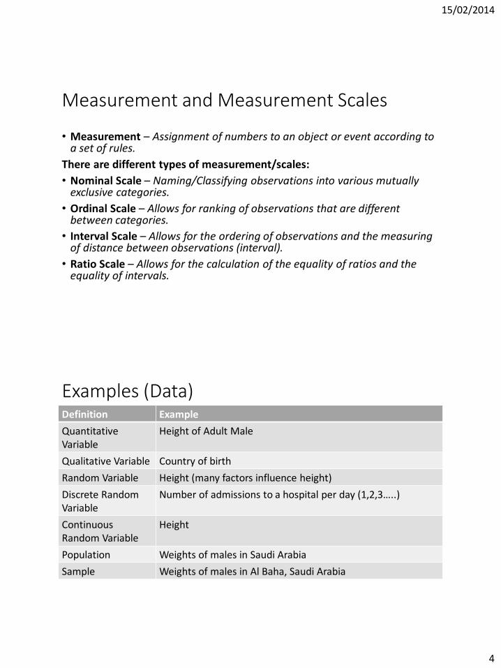
Measurement and Measurement Scales
• Measurement – Assignment of numbers to an object or event according to a set of rules.
There are different types of measurement/scales:
• Nominal Scale – Naming/Classifying observations into various mutually exclusive categories.
• Ordinal Scale – Allows for ranking of observations that are different between categories.
• Interval Scale – Allows for the ordering of observations and the measuring of distance between observations (interval).
• Ratio Scale – Allows for the calculation of the equality of ratios and the equality of intervals.
Examples (Data)Definition Example
Quantitative Variable
Height of Adult Male
Qualitative Variable Country of birth
Random Variable Height (many factors influence height)
Discrete Random Variable
Number of admissions to a hospital per day (1,2,3…..)
Continuous Random Variable
Height
Population Weights of males in Saudi Arabia
Sample Weights of males in Al Baha, Saudi Arabia
15/02/2014
5
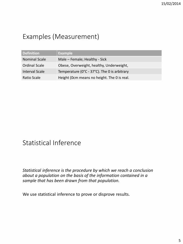
Examples (Measurement)
Definition Example
Nominal Scale Male – Female; Healthy - Sick
Ordinal Scale Obese, Overweight, healthy, Underweight,
Interval Scale Temperature (0°C - 37°C). The 0 is arbitrary
Ratio Scale Height (0cm means no height. The 0 is real.
Statistical Inference
Statistical inference is the procedure by which we reach a conclusion about a population on the basis of the information contained in a sample that has been drawn from that population.
We use statistical inference to prove or disprove results.
15/02/2014
6
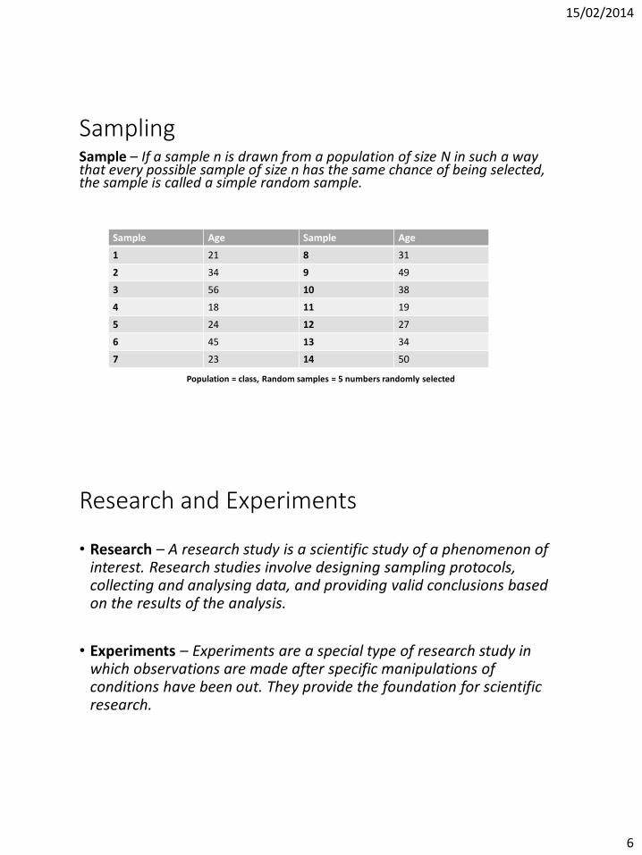
SamplingSample – If a sample n is drawn from a population of size N in such a way that every possible sample of size n has the same chance of being selected, the sample is called a simple random sample.
Population = class, Random samples = 5 numbers randomly selected
Sample Age Sample Age
1 21 8 31
2 34 9 49
3 56 10 38
4 18 11 19
5 24 12 27
6 45 13 34
7 23 14 50
Research and Experiments
• Research – A research study is a scientific study of a phenomenon of interest. Research studies involve designing sampling protocols, collecting and analysing data, and providing valid conclusions based on the results of the analysis.
• Experiments – Experiments are a special type of research study in which observations are made after specific manipulations of conditions have been out. They provide the foundation for scientific research.
15/02/2014
7
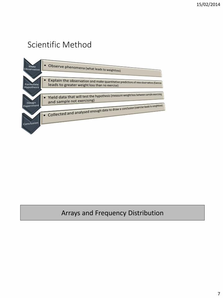
Scientific Method
Arrays and Frequency Distribution
15/02/2014
8
Revision
•Give examples of sources of data.
•Write down the steps of the scientific process.
•Give an example of a qualitative variable.
•What do we mean by the ordinal scale.
Descriptive Statistics. (Chapter 2)
•Arrays
•Frequency
•Distribution
•Stem and Leaf Displays/ Diagrams
15/02/2014
9
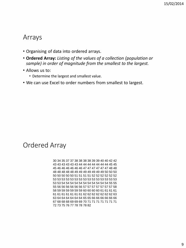
Arrays
• Organising of data into ordered arrays.
• Ordered Array: Listing of the values of a collection (population or sample) in order of magnitude from the smallest to the largest.
• Allows us to: • Determine the largest and smallest value.
• We can use Excel to order numbers from smallest to largest.
30 34 35 37 37 38 38 38 38 39 39 40 40 42 42
43 43 43 43 43 43 44 44 44 44 44 44 44 45 45
45 46 46 46 46 46 46 47 47 47 47 47 47 48 48
48 48 48 48 48 49 49 49 49 49 49 49 50 50 50
50 50 50 50 50 51 51 51 51 52 52 52 52 52 52
53 53 53 53 53 53 53 53 53 53 53 53 53 53 53
53 53 54 54 54 54 54 54 54 54 54 54 54 55 55
55 56 56 56 56 56 56 57 57 57 57 57 57 57 58
58 59 59 59 59 59 59 60 60 60 60 61 61 61 61
61 61 61 61 61 61 61 62 62 62 62 62 62 62 63
63 64 64 64 64 64 64 65 65 66 66 66 66 66 66
67 68 68 68 69 69 69 70 71 71 71 71 71 71 7172 73 75 76 77 78 78 78 82
Ordered Array
15/02/2014
10
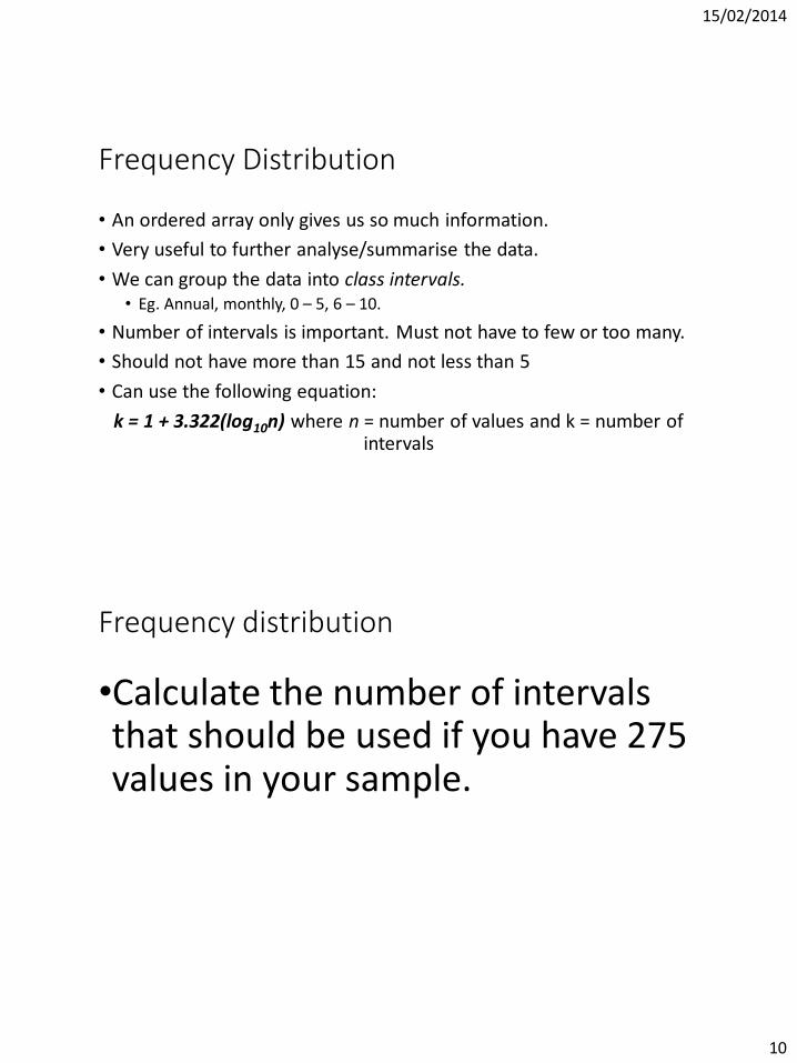
Frequency Distribution
• An ordered array only gives us so much information.
• Very useful to further analyse/summarise the data.
• We can group the data into class intervals. • Eg. Annual, monthly, 0 – 5, 6 – 10.
• Number of intervals is important. Must not have to few or too many.
• Should not have more than 15 and not less than 5
• Can use the following equation:
k = 1 + 3.322(log10n) where n = number of values and k = number of intervals
Frequency distribution
•Calculate the number of intervals that should be used if you have 275 values in your sample.
15/02/2014
11
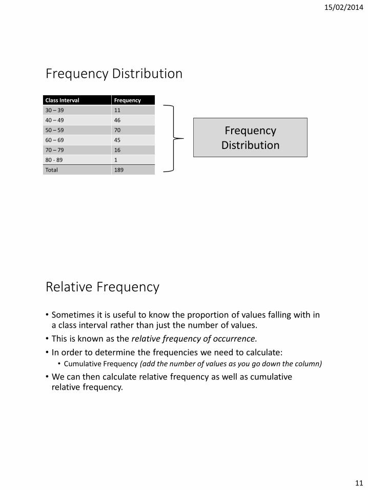
Frequency Distribution
Class Interval Frequency
30 – 39 11
40 – 49 46
50 – 59 70
60 – 69 45
70 – 79 16
80 - 89 1
Total 189
Frequency Distribution
Relative Frequency
• Sometimes it is useful to know the proportion of values falling with in a class interval rather than just the number of values.
• This is known as the relative frequency of occurrence.
• In order to determine the frequencies we need to calculate:• Cumulative Frequency (add the number of values as you go down the column)
• We can then calculate relative frequency as well as cumulative relative frequency.
15/02/2014
12
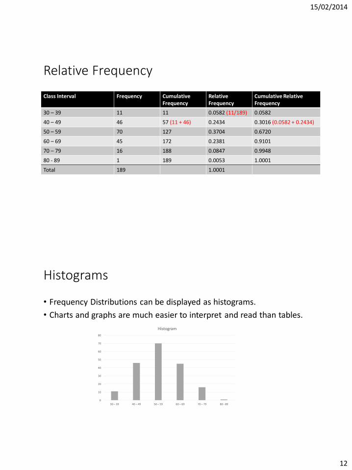
Relative Frequency
Class Interval Frequency Cumulative Frequency
Relative Frequency
Cumulative Relative Frequency
30 – 39 11 11 0.0582 (11/189) 0.0582
40 – 49 46 57 (11 + 46) 0.2434 0.3016 (0.0582 + 0.2434)
50 – 59 70 127 0.3704 0.6720
60 – 69 45 172 0.2381 0.9101
70 – 79 16 188 0.0847 0.9948
80 - 89 1 189 0.0053 1.0001
Total 189 1.0001
Histograms
• Frequency Distributions can be displayed as histograms.
• Charts and graphs are much easier to interpret and read than tables.
0
10
20
30
40
50
60
70
80
30 – 39 40 – 49 50 – 59 60 – 69 70 – 79 80 - 89
Histogram
15/02/2014
13
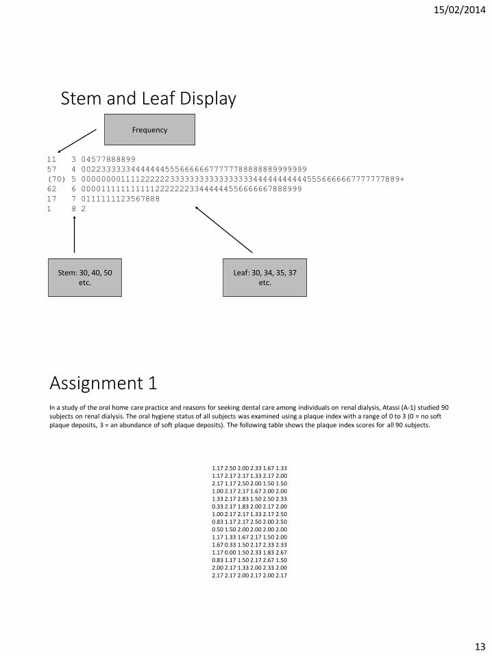
Stem and Leaf Display
11 3 04577888899
57 4 0022333333444444455566666677777788888889999999
(70) 5 00000000111122222233333333333333333444444444445556666667777777889+
62 6 000011111111111222222233444444556666667888999
17 7 0111111123567888
1 8 2
Stem: 30, 40, 50 etc.
Leaf: 30, 34, 35, 37 etc.
Frequency
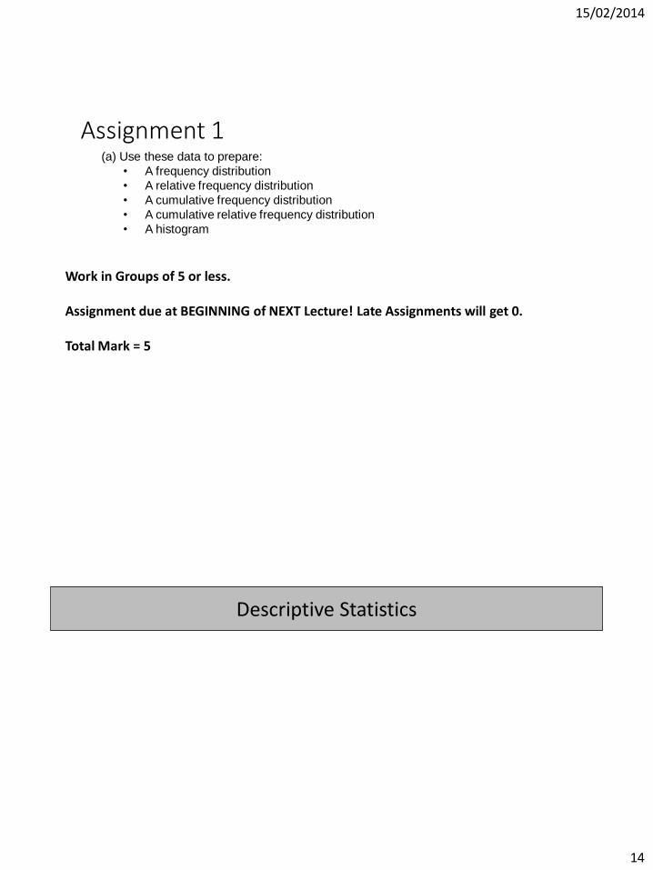
Assignment 1In a study of the oral home care practice and reasons for seeking dental care among individuals on renal dialysis, Atassi (A-1) studied 90 subjects on renal dialysis. The oral hygiene status of all subjects was examined using a plaque index with a range of 0 to 3 (0 = no soft plaque deposits, 3 = an abundance of soft plaque deposits). The following table shows the plaque index scores for all 90 subjects.
1.17 2.50 2.00 2.33 1.67 1.331.17 2.17 2.17 1.33 2.17 2.002.17 1.17 2.50 2.00 1.50 1.501.00 2.17 2.17 1.67 2.00 2.001.33 2.17 2.83 1.50 2.50 2.330.33 2.17 1.83 2.00 2.17 2.001.00 2.17 2.17 1.33 2.17 2.500.83 1.17 2.17 2.50 2.00 2.500.50 1.50 2.00 2.00 2.00 2.001.17 1.33 1.67 2.17 1.50 2.001.67 0.33 1.50 2.17 2.33 2.331.17 0.00 1.50 2.33 1.83 2.670.83 1.17 1.50 2.17 2.67 1.502.00 2.17 1.33 2.00 2.33 2.002.17 2.17 2.00 2.17 2.00 2.17
15/02/2014
14
(a) Use these data to prepare:
• A frequency distribution
• A relative frequency distribution
• A cumulative frequency distribution
• A cumulative relative frequency distribution
• A histogram
Assignment 1
Work in Groups of 5 or less.
Assignment due at BEGINNING of NEXT Lecture! Late Assignments will get 0.
Total Mark = 5
Descriptive Statistics
15/02/2014
15
Descriptive Statistics Cont. (Chapter 2)
• Mean
• Median
• Mode
• Dispersion
• Standard Deviation
• Coefficient of Variation
• Percentiles
• Quartiles
• Box and Whisker Plot
Measures of Central Tendency
• Sometimes we just want a single number to describe the data. This is called a descriptive tendency.
• Statistic: A descriptive measure computed from the data of a sample.
• Parameter: A descriptive measure computed from the data of a population.
• Most common measures of central tendency are: • Mean, Median and Mode
15/02/2014
16
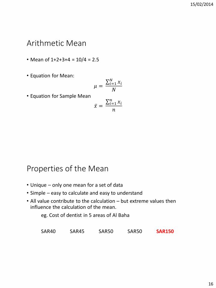
Arithmetic Mean
• Mean of 1+2+3+4 = 10/4 = 2.5
• Equation for Mean:
𝜇 = 𝑖=1𝑁 𝑥𝑖𝑁
• Equation for Sample Mean
𝑥 = 𝑖=1𝑛 𝑥𝑖𝑛
Properties of the Mean
• Unique – only one mean for a set of data
• Simple – easy to calculate and easy to understand
• All value contribute to the calculation – but extreme values then influence the calculation of the mean.
eg. Cost of dentist in 5 areas of Al Baha
SAR40 SAR45 SAR50 SAR50 SAR150
15/02/2014
17
Median
• Divides data into two sets of equal size in the middle.
• Eg.
1 2 3 4 5 6 7 = 4 (Middle)
1 2 3 4 5 6 7 8 = (9/2) Middle two numbers)
IMPORTANT – Numbers must be ranked (smallest to largest)
Properties of the Median
• Unique and easy to understand
• Simple to calculate
• Not really effected by extreme values.
15/02/2014
18
Mode
• The value in the dataset that occurs most frequently
• Eg.
1 1 2 2 2 3 4 4 5
The mode = 2 (occurs 3 times)
A dataset can have no mode or more than one mode.
Measures of dispersion
• Dispersion = variety = differences.
• Measures of dispersion include:• Range
• Variance
• Standard deviation
• Coeffecient of variation
• Percentiles
• Quartiles
• Interquartile range
15/02/2014
19
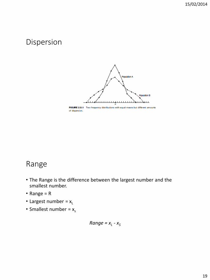
Dispersion
Range
• The Range is the difference between the largest number and the smallest number.
• Range = R
• Largest number = xL
• Smallest number = xs
Range = xL - xS
15/02/2014
20
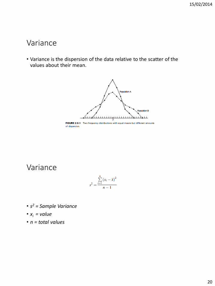
Variance
• Variance is the dispersion of the data relative to the scatter of the values about their mean.
Variance
• s2 = Sample Variance
• xi = value
• n = total values
15/02/2014
21
Standard Deviation
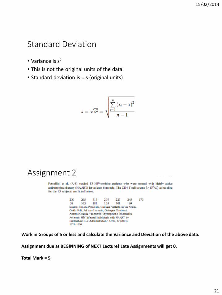
• Variance is s2
• This is not the original units of the data
• Standard deviation is = s (original units)
Assignment 2
Work in Groups of 5 or less and calculate the Variance and Deviation of the above data.
Assignment due at BEGINNING of NEXT Lecture! Late Assignments will get 0.
Total Mark = 5
15/02/2014
22
Descriptive Statistics Continued
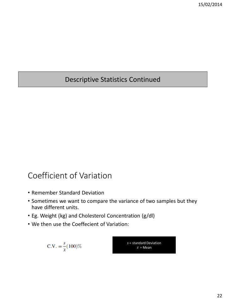
Coefficient of Variation
• Remember Standard Deviation
• Sometimes we want to compare the variance of two samples but they have different units.
• Eg. Weight (kg) and Cholesterol Concentration (g/dl)
• We then use the Coeffecient of Variation:
s = standard Deviation= Mean
15/02/2014
23
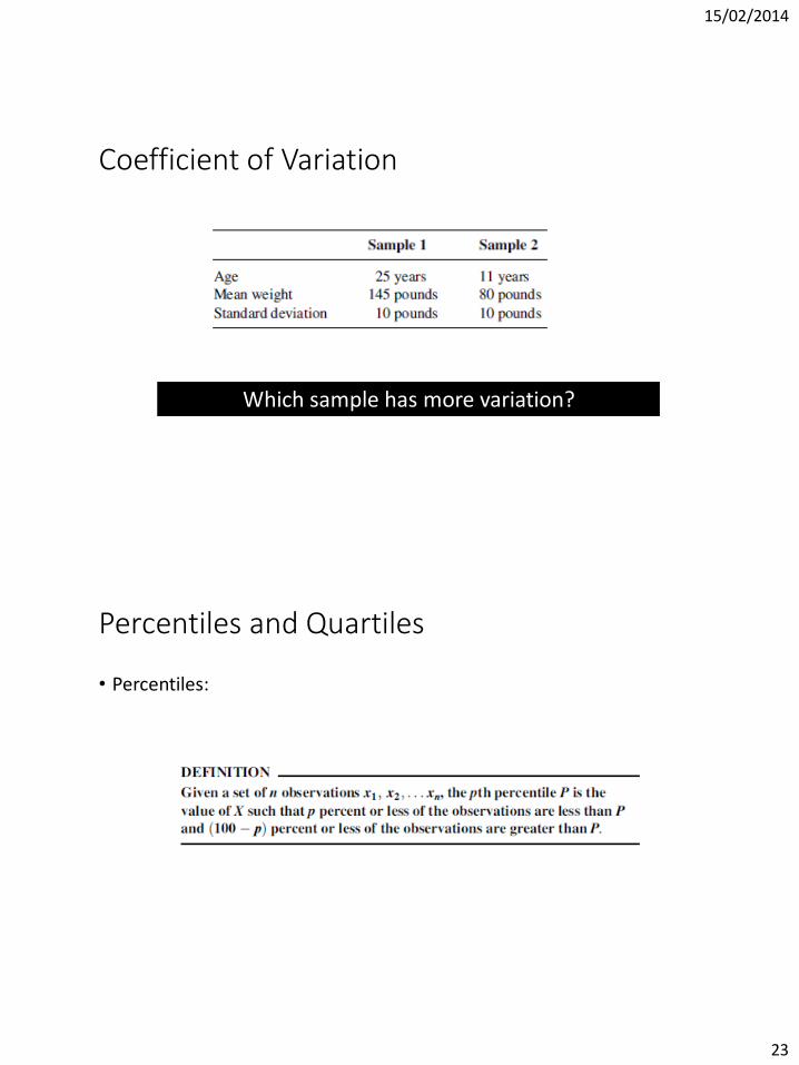
Coefficient of Variation
Which sample has more variation?
Percentiles and Quartiles
• Percentiles:
15/02/2014
24
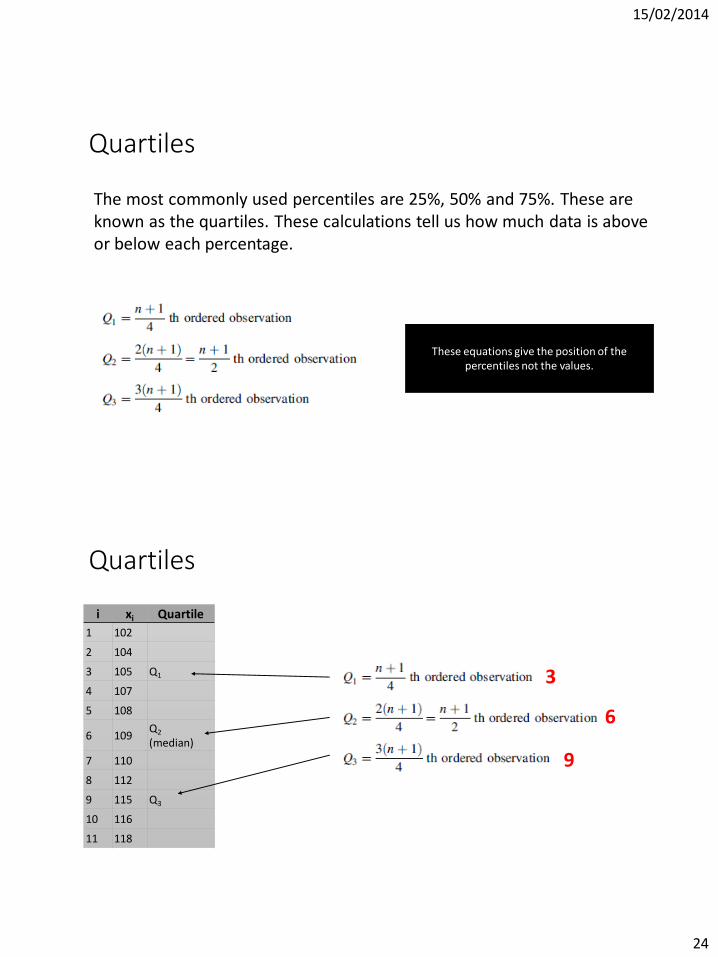
Quartiles
These equations give the position of the percentiles not the values.
The most commonly used percentiles are 25%, 50% and 75%. These are known as the quartiles. These calculations tell us how much data is above or below each percentage.
Quartiles
i xi Quartile
1 102
2 104
3 105 Q1
4 107
5 108
6 109Q2
(median)
7 110
8 112
9 115 Q3
10 116
11 118
3
6
9
15/02/2014
25
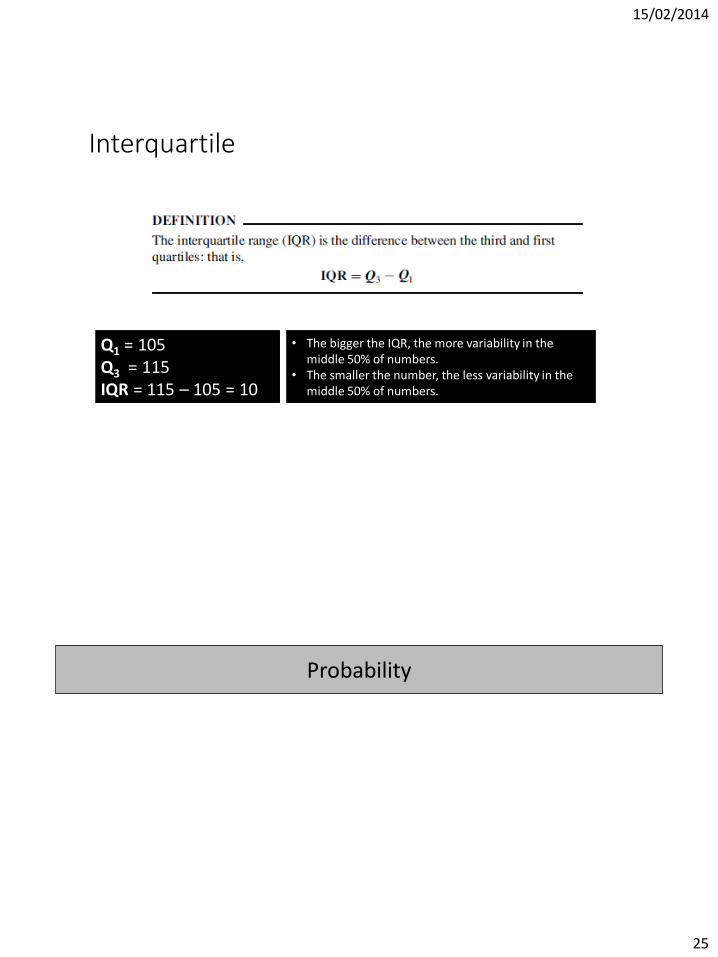
Interquartile
Q1 = 105Q3 = 115IQR = 115 – 105 = 10
• The bigger the IQR, the more variability in the middle 50% of numbers.
• The smaller the number, the less variability in the middle 50% of numbers.
Probability
15/02/2014
26
Introduction
1. Given some process (or experiment) with n mutually exclusive outcomes (called events), E1, E2…….En, the probability of any event Ei is assigned a non-negative number.
P(Ei) ≥ 0
Mutually Elusive: Events cannot occur simultaneously.
Introduction
15/02/2014
27
Introduction
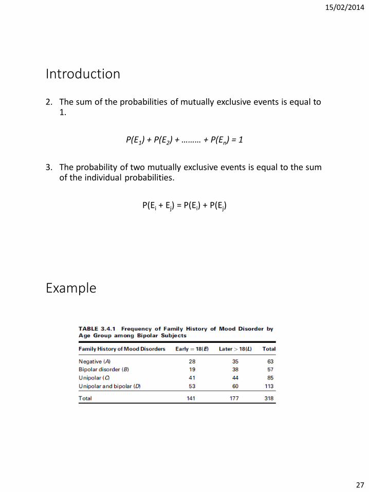
2. The sum of the probabilities of mutually exclusive events is equal to 1.
P(E1) + P(E2) + ……… + P(En) = 1
3. The probability of two mutually exclusive events is equal to the sum of the individual probabilities.
P(Ei + Ej) = P(Ei) + P(Ej)
Example
15/02/2014
28
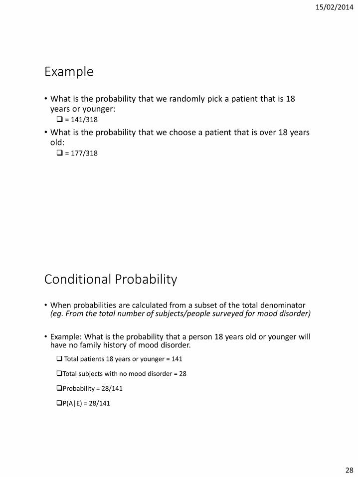
Example
• What is the probability that we randomly pick a patient that is 18 years or younger: = 141/318
• What is the probability that we choose a patient that is over 18 years old: = 177/318
Conditional Probability
• When probabilities are calculated from a subset of the total denominator (eg. From the total number of subjects/people surveyed for mood disorder)
• Example: What is the probability that a person 18 years old or younger will have no family history of mood disorder.
Total patients 18 years or younger = 141
Total subjects with no mood disorder = 28
Probability = 28/141
P(A|E) = 28/141
15/02/2014
29
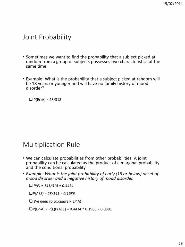
Joint Probability
• Sometimes we want to find the probability that a subject picked at random from a group of subjects possesses two characteristics at the same time.
• Example: What is the probability that a subject picked at random will be 18 years or younger and will have no family history of mood disorder?
P(E∩A) = 28/318
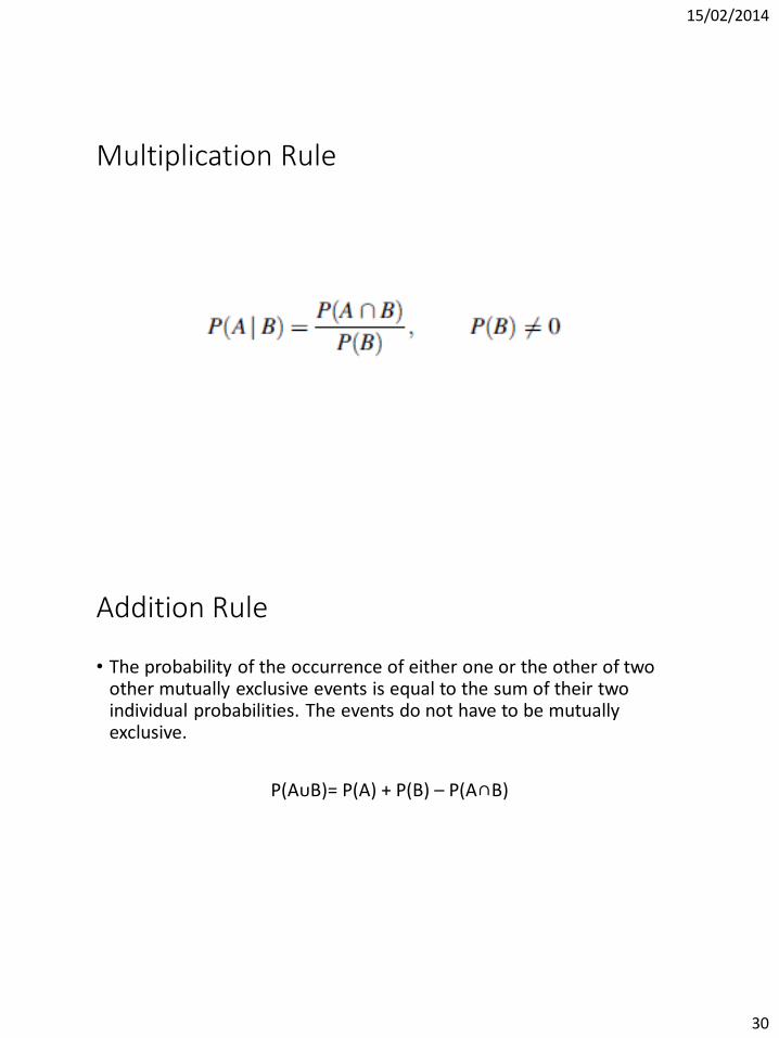
Multiplication Rule
• We can calculate probabilities from other probabilities. A joint probability can be calculated as the product of a marginal probability and the conditional probability
• Example: What is the joint probability of early (18 or below) onset of mood disorder and a negative history of mood disorder.
P(E) = 141/318 = 0.4434
P(A|E) = 28/141 = 0.1986
We need to calculate P(E∩A)
P(E∩A) = P(E)P(A|E) = 0.4434 * 0.1986 = 0.0881
15/02/2014
30
Multiplication Rule
Addition Rule
• The probability of the occurrence of either one or the other of two other mutually exclusive events is equal to the sum of their two individual probabilities. The events do not have to be mutually exclusive.
P(AᴜB)= P(A) + P(B) – P(A∩B)
15/02/2014
31
Addition Rule
• Example: If we pick a person at random what is the probability that this person will have early stage onset of mood disorder or will have no family history of mood disorders or both.
P(EᴜA)= P(E) + P(A) – P(E∩A)
• P(E) = 141/318 = 0.4434
• P(E∩A) = 28/318 = 0.0881
• P(A) = 63/318 = 0.1981
• P(EᴜA) = 0.4434 + 0.1981 – 0.0881 = 0.05534
Independent Events
• A and B are independent events if the probability of event A happening is the same whether event B occurs or not.
• You use the multiplication rule in this case:
P(A∩B) = P(A)P(B)
15/02/2014
32
Independent Events
• In a high school with 60 girls and 40 boys, 24 girls and 16 boys where glasses. What is the probability that a student picked at random is a boy and wears eye glasses.
• Being a boy and wearing eye glasses are independent.
P(B∩E) = P(B)P(E)
• P(B) = 16/40 = 0.4
• P(E) = 40/100 = 0.4
• P(B∩E) = 0.4 * 0.4 = 0.16
Complementary Events
• Complementary events are mutually exclusive.
• Example: Being early stage onset is mutually exclusive for late stage onset.
P(Ā) = 1 – P(A)
15/02/2014
33
Complementary Events
• Example: If there are 1200 admissions to a hospital and 750 admissions are private then 450 patients must be state patients. So:
• P(A) = 750/1200 = 0.625
• Then P(Ā) = 1 – P(A) = 1 – 0.625 = 0.375
• Therefore the probability of a patient being a state patient is 0.375
Bayes Theorem
15/02/2014
34
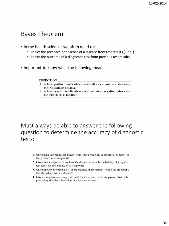
Bayes Theorem
• In the health sciences we often need to:• Predict the presence or absence of a disease from test results (+ or -)
• Predict the outcome of a diagnostic test from previous test results
• Important to know what the following mean:
Must always be able to answer the following question to determine the accuracy of diagnostic tests:
15/02/2014
35
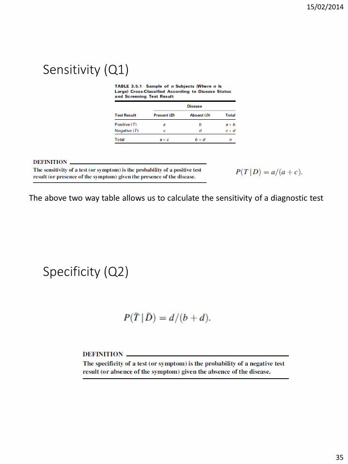
Sensitivity (Q1)
The above two way table allows us to calculate the sensitivity of a diagnostic test
Specificity (Q2)
15/02/2014
36
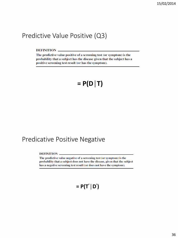
Predictive Value Positive (Q3)
= P(D│T)
Predicative Positive Negative
= P(T’│D’)
15/02/2014
37
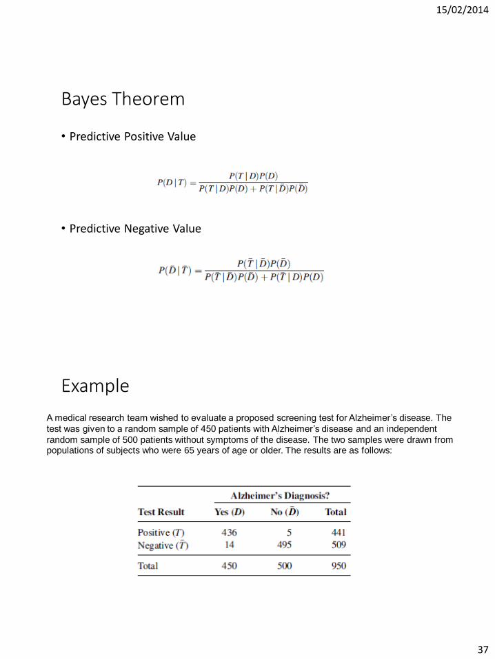
Bayes Theorem
• Predictive Positive Value
• Predictive Negative Value
Example
A medical research team wished to evaluate a proposed screening test for Alzheimer’s disease. The
test was given to a random sample of 450 patients with Alzheimer’s disease and an independent
random sample of 500 patients without symptoms of the disease. The two samples were drawn from populations of subjects who were 65 years of age or older. The results are as follows:
15/02/2014
38
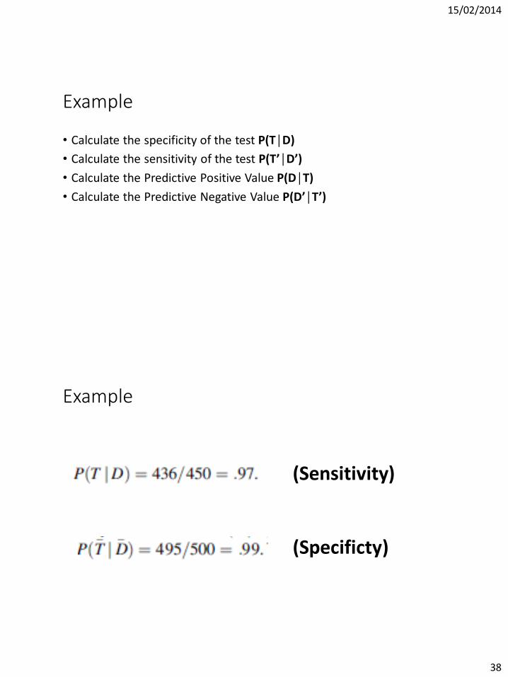
Example
• Calculate the specificity of the test P(T│D)
• Calculate the sensitivity of the test P(T’│D’)
• Calculate the Predictive Positive Value P(D│T)
• Calculate the Predictive Negative Value P(D’│T’)
Example
(Sensitivity)
(Specificty)
15/02/2014
39
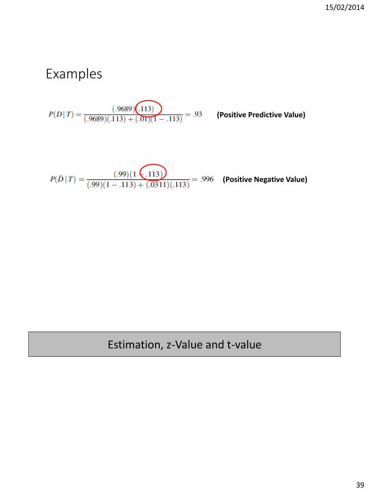
Examples
(Positive Predictive Value)
(Positive Negative Value)
Estimation, z-Value and t-value
15/02/2014
40
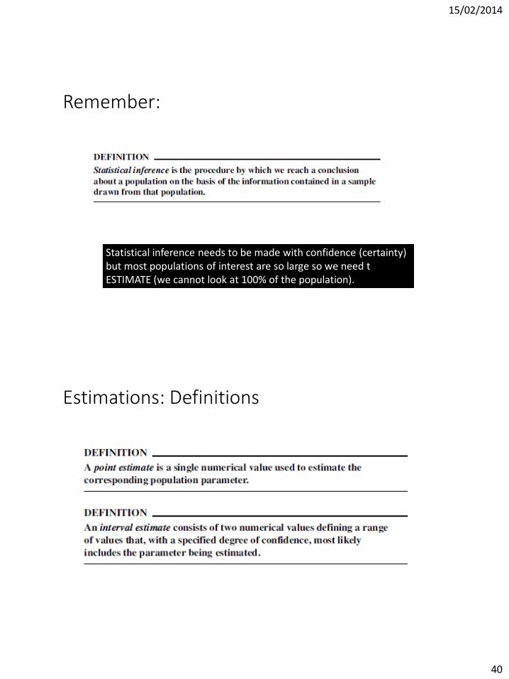
Remember:
Statistical inference needs to be made with confidence (certainty) but most populations of interest are so large so we need t ESTIMATE (we cannot look at 100% of the population).
Estimations: Definitions
15/02/2014
41
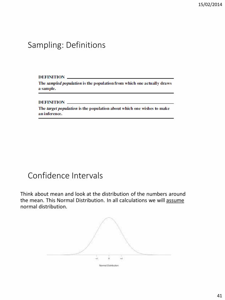
Sampling: Definitions
Confidence Intervals
Think about mean and look at the distribution of the numbers around the mean. This Normal Distribution. In all calculations we will assume normal distribution.
15/02/2014
42
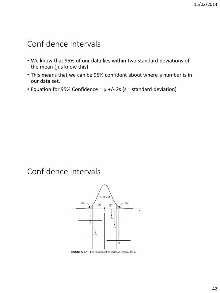
Confidence Intervals
• We know that 95% of our data lies within two standard deviations of the mean (jus know this)
• This means that we can be 95% confident about where a number is in our data set.
• Equation for 95% Confidence = μ +/- 2s (s = standard deviation)
Confidence Intervals
15/02/2014
43
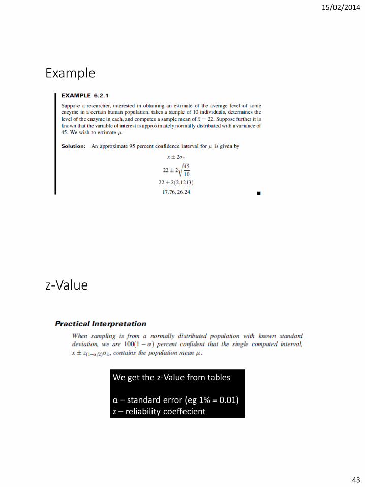
Example
z-Value
We get the z-Value from tables
α – standard error (eg 1% = 0.01)z – reliability coeffecient
15/02/2014
44
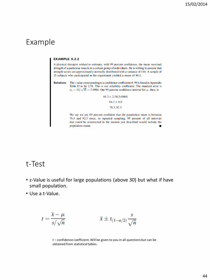
Example
t-Test
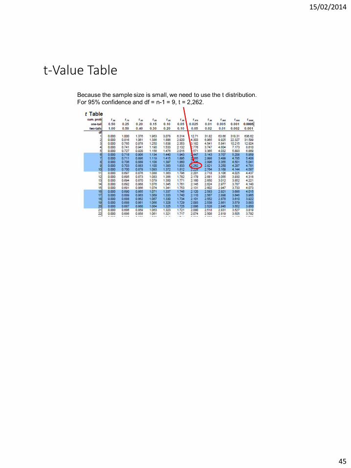
• z-Value is useful for large populations (above 30) but what if have small population.
• Use a t-Value.
t – confidence coefficient. Will be given to you in all questions but can be obtained from statistical tables.
15/02/2014
45
t-Value Table


