BIOS 312: MODERN REGRESSION ANALYSIS -...
41
B IOS 312: M ODERN R EGRESSION A NALYSIS James C (Chris) Slaughter Department of Biostatistics Vanderbilt University School of Medicine [email protected] biostat.mc.vanderbilt.edu/CourseBios312 Copyright 2009-2012 JC Slaughter All Rights Reserved Updated January 5, 2012
Transcript of BIOS 312: MODERN REGRESSION ANALYSIS -...

BIOS 312: MODERN REGRESSION ANALYSIS
James C (Chris) SlaughterDepartment of Biostatistics
Vanderbilt University School of [email protected]
biostat.mc.vanderbilt.edu/CourseBios312
Copyright 2009-2012 JC Slaughter All Rights ReservedUpdated January 5, 2012
Contents
7 Adjustment for Covariates 4
7.1 Overview . . . . . . . . . . . . . . . . . . . . . . . . . . . . . . . . 4
7.2 Stratified Analysis . . . . . . . . . . . . . . . . . . . . . . . . . . . 7
7.2.1 Methods . . . . . . . . . . . . . . . . . . . . . . . . . . . . . 7
7.2.2 Weights for Effect Modification . . . . . . . . . . . . . . . . 8
7.2.3 Weights for Confounders and Precision Variables . . . . . . 10
7.3 Multivariable Regression . . . . . . . . . . . . . . . . . . . . . . . . 15
7.3.1 General Regression Setting . . . . . . . . . . . . . . . . . . 15
7.3.2 General Uses of Multivariable Regression . . . . . . . . . . 17
7.3.3 Software . . . . . . . . . . . . . . . . . . . . . . . . . . . . 19
7.3.4 Example: FEV and Smoking . . . . . . . . . . . . . . . . . 19
7.4 Unadjusted versus Adjusted Models . . . . . . . . . . . . . . . . . 21
7.4.1 General comparison . . . . . . . . . . . . . . . . . . . . . . 21
7.4.2 Comparison of Adjusted and Unadjusted Models in LinearRegression . . . . . . . . . . . . . . . . . . . . . . . . . . . 23
3
CONTENTS 4
7.4.3 Precision variables . . . . . . . . . . . . . . . . . . . . . . . 26
7.4.4 Confounding variables . . . . . . . . . . . . . . . . . . . . . 29
7.4.5 Variance Inflation . . . . . . . . . . . . . . . . . . . . . . . . 30
7.4.6 Irrelevant variables . . . . . . . . . . . . . . . . . . . . . . . 31
7.5 Example: FEV and Smoking in Children . . . . . . . . . . . . . . . 31
7.5.1 Linear model for geometric means . . . . . . . . . . . . . . 31
7.5.2 Logistic model . . . . . . . . . . . . . . . . . . . . . . . . . 38

Chapter 7
Adjustment for Covariates
7.1 Overview
· Scientific questions
– Most often scientific questions are translated into comparing the distribu-tion of some response variable across groups of interest
– Groups are defined by the predictor of interest (POI)∗ Categorical predictors of interest: Treatment or control, knockout or
wild type, ethnic group
∗ Continuous predictors of interest: Age, BMI, cholesterol, blood pres-sure
· If we only considered the response and POI, this is referred to as a simple(linear, logistic, PH, etc.) regression model
· Often we need to consider additional variables other than POI because...
– We want to make comparisons in different strata
5

CHAPTER 7. ADJUSTMENT FOR COVARIATES 6
∗ e.g if we stratify by gender, we may get different answers to our scien-tific question in men and women
– Groups being compared differ in other ways∗ Confounding: A variable that is related to both the outcome and pre-
dictor of interest
– Less variability in the response if we control for other variables∗ Precision: If we restrict to looking within certain strata, may get smallerσ2
· Statistics: Covariates other than the Predictor of Interest are included in themodel as...
– Effect modifiers
– Confounders
– Precision variables
· Two main statistical methods to adjust for covariates
– Stratified analyses∗ Combines information about associations between response across
strata
∗ Will not borrow information about (or even estimate) associations be-tween response and adjustment variables
– Adjustment in multiple regression∗ Can (but does not have to) borrow information about associations be-
tween response and all modeled variables
∗ Could conduct a stratified analysis using regression
CHAPTER 7. ADJUSTMENT FOR COVARIATES 7
∗ In practice, when researchers say they are using regression, they arealmost certainly doing so to borrow information
· Example: Is smoking associated with FEV in teenagers?
– Stratified Analysis∗ Separately estimate mean FEV in 19 year olds, 18 year olds, 17 year
olds, etc. by smoking status
∗ Average means (using weights) to come up with overall effect of smok-ing on FEV
∗ Key: Not trying to estimate a common effect of age across strata (notborrowing information across age)
∗ No estimate of the age effect in this analysis
– Multiple regression∗ Fit a regression model with FEV as the outcome, smoking as the POI,
and age as an adjustment variable
∗ Will provide you an estimate of the association between FEV and age(but do you care?)
∗ Can borrow information across ages to estimate the age effect· Linear/spline function for age would borrow information
· Separate indicator variable for each age would borrow less infor-mation (would still assume that all 19.1 and 19.2 year olds are thesame)
· Adjustment for two factors: Age and Sex
– Stratified analyses

CHAPTER 7. ADJUSTMENT FOR COVARIATES 8
∗ Calculate separate means by age and sex, combine using weight av-erages as before
∗ This method adjusts for the interaction of age and sex (in addition toage and sex main effects)
– Multiple regression∗ “We adjusted for age and sex...” or “Holding age and sex constant, we
found ...”
∗ Almost certainly the research adjusted for age and sex, but not theinteraction of the two variables (but they could have)
7.2 Stratified Analysis
7.2.1 Methods
· General approach to conducting a stratified analysis
– Divide the data into strata based on all combinations of the “adjustment”covariates∗ e.g. every combination of age, gender, race, SES, etc.
– Within each strata, perform an analysis comparing responses across POIgroups
– Use (weighted) average of estimated associations across groups
· Combining responses: Easy if estimates are independent and approximatelyNormally distributed
– For independent strata k, k = 1, . . . , K
∗ Estimate in stratum k: θk ∼ N(θk, se2k)
CHAPTER 7. ADJUSTMENT FOR COVARIATES 9
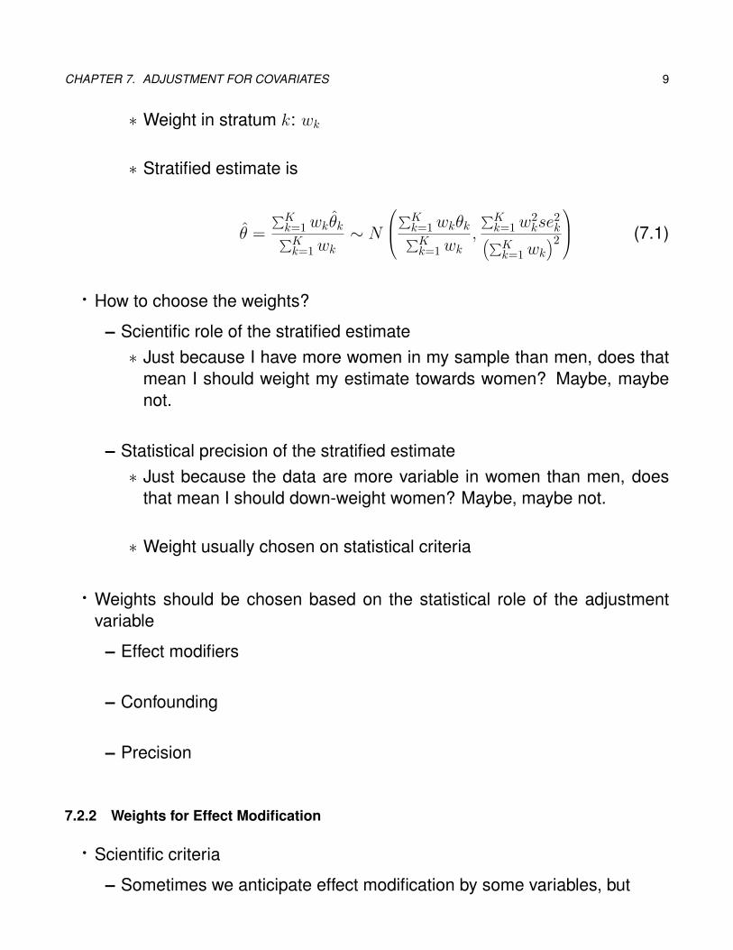
∗ Weight in stratum k: wk
∗ Stratified estimate is
θ =
∑Kk=1wkθk∑Kk=1wk
∼ N
∑Kk=1wkθk∑Kk=1wk
,
∑Kk=1w
2kse
2k(∑K
k=1wk)2 (7.1)
· How to choose the weights?
– Scientific role of the stratified estimate∗ Just because I have more women in my sample than men, does that
mean I should weight my estimate towards women? Maybe, maybenot.
– Statistical precision of the stratified estimate∗ Just because the data are more variable in women than men, does
that mean I should down-weight women? Maybe, maybe not.
∗ Weight usually chosen on statistical criteria
· Weights should be chosen based on the statistical role of the adjustmentvariable
– Effect modifiers
– Confounding
– Precision
7.2.2 Weights for Effect Modification
· Scientific criteria
– Sometimes we anticipate effect modification by some variables, but
CHAPTER 7. ADJUSTMENT FOR COVARIATES 10
∗ We do not choose to report estimates of the association between theresponse and POI in each stratum separately· e.g. political polls, age adjusted incidence rates
∗ We are interested in estimating the “average association” for a popu-lation
· Choosing weights according to scientific importance
– Want to estimate the average effect in some population of interest∗ The real population, or,
∗ Some standard population used for comparisons
– Example: Ecologic studies comparing incidence of hip fractures acrosscountries∗ Hip fracture rates increase with age
∗ Industrialized countries and developing world have very different agedistributions
∗ Choose a standard age distribution to remove confounding by age
· Comment on oversampling
– In political polls or epidemiologic studies we sometimes oversample somestrata in order to gain precision∗ For fixed maximal sample size, we gain most precision if stratum sam-
ples size is proportional to weight times standard deviation of mea-surements in stratum
∗ Example: Oversample swing-voters relative to individuals who we canbe more certain about their voting preferences

CHAPTER 7. ADJUSTMENT FOR COVARIATES 11
– For independent strata k, k = 1, . . . , K
∗ Sample size in stratum k: nk
∗ Estimate in stratum k: θk ∼ N(θk, se
2k =
Vknk
)
∗ Importance weight for stratum k: wk
∗ Optimal sample size when N =∑Kk=1 nk is:
w1
√V1
n1=w2
√V2
n2= . . . =
wk√Vk
nk(7.2)
7.2.3 Weights for Confounders and Precision Variables
· If the true association is the same in each stratum, we are free to considerstatistical criteria
– It is very unlikely that there is no effect modification in truth, but is it smallenough to ignore?
· Statistical criteria
– Maximize precision of stratified estimates by minimizing the standard er-ror
· Optimal statistical weights
– For independent strata k, k = 1, . . . , K
∗ Sample size in stratum k: nk
∗ Estimate in stratum k: θk ∼ N(θk, se
2k =
Vknk
)
∗ Importance weight for stratum k: wk
CHAPTER 7. ADJUSTMENT FOR COVARIATES 12
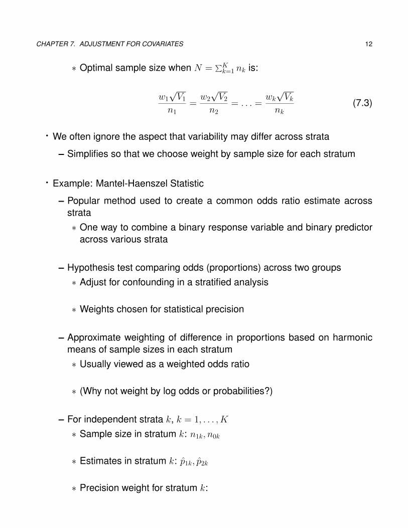
∗ Optimal sample size when N =∑Kk=1 nk is:
w1
√V1
n1=w2
√V2
n2= . . . =
wk√Vk
nk(7.3)
· We often ignore the aspect that variability may differ across strata
– Simplifies so that we choose weight by sample size for each stratum
· Example: Mantel-Haenszel Statistic
– Popular method used to create a common odds ratio estimate acrossstrata∗ One way to combine a binary response variable and binary predictor
across various strata
– Hypothesis test comparing odds (proportions) across two groups∗ Adjust for confounding in a stratified analysis
∗ Weights chosen for statistical precision
– Approximate weighting of difference in proportions based on harmonicmeans of sample sizes in each stratum∗ Usually viewed as a weighted odds ratio
∗ (Why not weight by log odds or probabilities?)
– For independent strata k, k = 1, . . . , K
∗ Sample size in stratum k: n1k, n0k
∗ Estimates in stratum k: p1k, p2k
∗ Precision weight for stratum k:
CHAPTER 7. ADJUSTMENT FOR COVARIATES 13
wk =n1kn0kn1k + n0k
÷K∑k=1
n1kn0kn1k + n0k
(7.4)
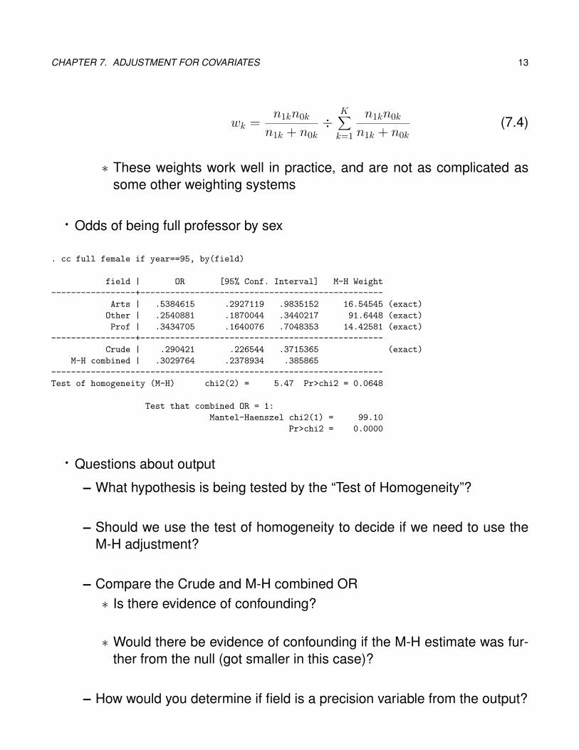
∗ These weights work well in practice, and are not as complicated assome other weighting systems
· Odds of being full professor by sex
. cc full female if year==95, by(field)
field | OR [95% Conf. Interval] M-H Weight
-----------------+-------------------------------------------------
Arts | .5384615 .2927119 .9835152 16.54545 (exact)
Other | .2540881 .1870044 .3440217 91.6448 (exact)
Prof | .3434705 .1640076 .7048353 14.42581 (exact)
-----------------+-------------------------------------------------
Crude | .290421 .226544 .3715365 (exact)
M-H combined | .3029764 .2378934 .385865
-------------------------------------------------------------------
Test of homogeneity (M-H) chi2(2) = 5.47 Pr>chi2 = 0.0648
Test that combined OR = 1:
Mantel-Haenszel chi2(1) = 99.10
Pr>chi2 = 0.0000
· Questions about output
– What hypothesis is being tested by the “Test of Homogeneity”?
– Should we use the test of homogeneity to decide if we need to use theM-H adjustment?
– Compare the Crude and M-H combined OR∗ Is there evidence of confounding?
∗ Would there be evidence of confounding if the M-H estimate was fur-ther from the null (got smaller in this case)?
– How would you determine if field is a precision variable from the output?

CHAPTER 7. ADJUSTMENT FOR COVARIATES 14
· Can compare the M-H results to results obtained running logistic regression
Unadjusted OR from logistic regression
Logistic regression Number of obs = 1597
LR chi2(1) = 109.43
Prob > chi2 = 0.0000
Log likelihood = -1049.533 Pseudo R2 = 0.0495
------------------------------------------------------------------------------
full | Odds Ratio Std. Err. z P>|z| [95% Conf. Interval]
-------------+----------------------------------------------------------------
female | .290421 .035561 -10.10 0.000 .2284555 .3691939
------------------------------------------------------------------------------
CHAPTER 7. ADJUSTMENT FOR COVARIATES 15
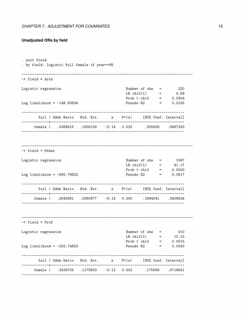
Unadjusted ORs by field
. sort field
. by field: logistic full female if year==95
----------------------------------------------------------------------------------
-> field = Arts
Logistic regression Number of obs = 220
LR chi2(1) = 4.69
Prob > chi2 = 0.0304
Log likelihood = -148.83634 Pseudo R2 = 0.0155
------------------------------------------------------------------------------
full | Odds Ratio Std. Err. z P>|z| [95% Conf. Interval]
-------------+----------------------------------------------------------------
female | .5384615 .1556108 -2.14 0.032 .305608 .9487343
------------------------------------------------------------------------------
----------------------------------------------------------------------------------
-> field = Other
Logistic regression Number of obs = 1067
LR chi2(1) = 91.17
Prob > chi2 = 0.0000
Log likelihood = -692.78622 Pseudo R2 = 0.0617
------------------------------------------------------------------------------
full | Odds Ratio Std. Err. z P>|z| [95% Conf. Interval]
-------------+----------------------------------------------------------------
female | .2540881 .0380877 -9.14 0.000 .1894041 .3408624
------------------------------------------------------------------------------
----------------------------------------------------------------------------------
-> field = Prof
Logistic regression Number of obs = 310
LR chi2(1) = 10.10
Prob > chi2 = 0.0015
Log likelihood = -202.74823 Pseudo R2 = 0.0243
------------------------------------------------------------------------------
full | Odds Ratio Std. Err. z P>|z| [95% Conf. Interval]
-------------+----------------------------------------------------------------
female | .3434705 .1175803 -3.12 0.002 .175589 .6718641
------------------------------------------------------------------------------
CHAPTER 7. ADJUSTMENT FOR COVARIATES 16
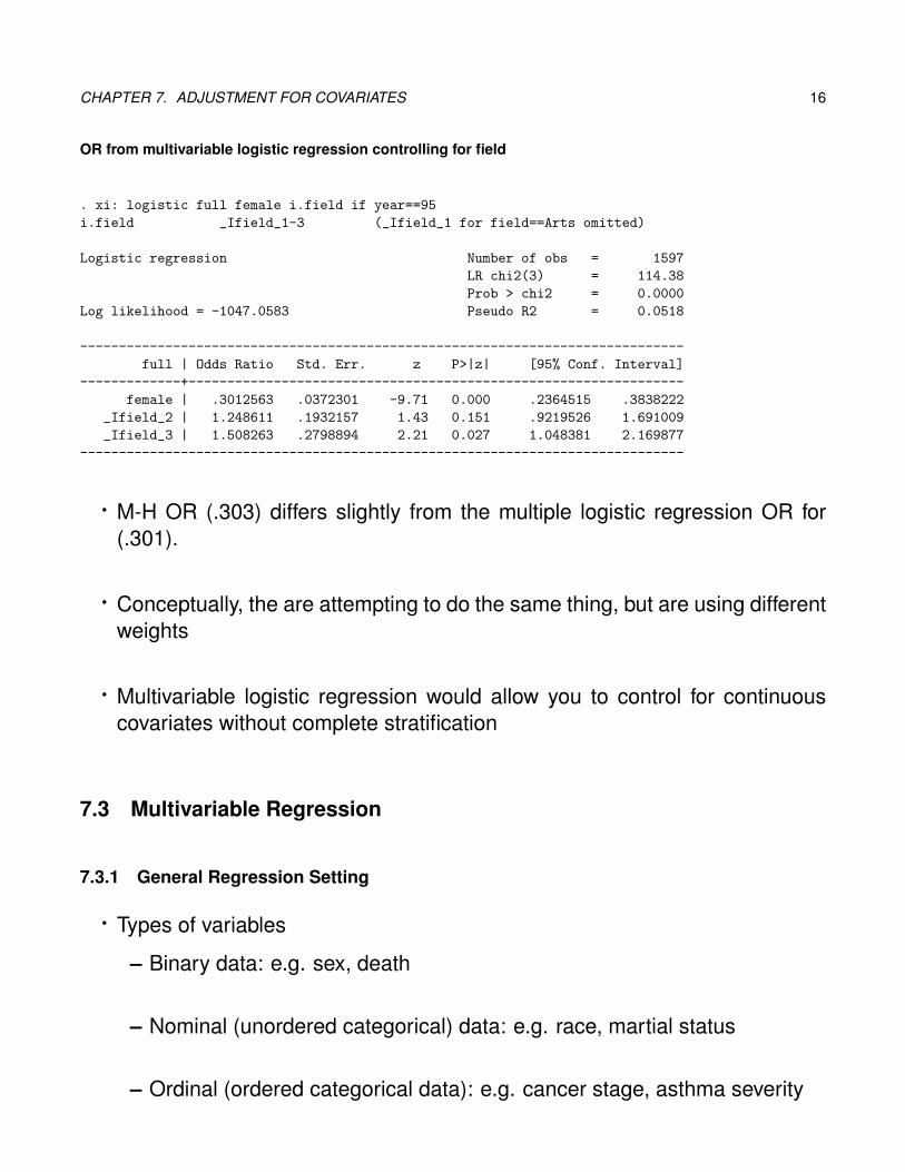
OR from multivariable logistic regression controlling for field
. xi: logistic full female i.field if year==95
i.field _Ifield_1-3 (_Ifield_1 for field==Arts omitted)
Logistic regression Number of obs = 1597
LR chi2(3) = 114.38
Prob > chi2 = 0.0000
Log likelihood = -1047.0583 Pseudo R2 = 0.0518
------------------------------------------------------------------------------
full | Odds Ratio Std. Err. z P>|z| [95% Conf. Interval]
-------------+----------------------------------------------------------------
female | .3012563 .0372301 -9.71 0.000 .2364515 .3838222
_Ifield_2 | 1.248611 .1932157 1.43 0.151 .9219526 1.691009
_Ifield_3 | 1.508263 .2798894 2.21 0.027 1.048381 2.169877
------------------------------------------------------------------------------
· M-H OR (.303) differs slightly from the multiple logistic regression OR for(.301).
· Conceptually, the are attempting to do the same thing, but are using differentweights
· Multivariable logistic regression would allow you to control for continuouscovariates without complete stratification
7.3 Multivariable Regression
7.3.1 General Regression Setting
· Types of variables
– Binary data: e.g. sex, death
– Nominal (unordered categorical) data: e.g. race, martial status
– Ordinal (ordered categorical data): e.g. cancer stage, asthma severity
CHAPTER 7. ADJUSTMENT FOR COVARIATES 17
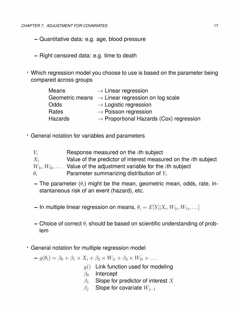
– Quantitative data: e.g. age, blood pressure
– Right censored data: e.g. time to death
· Which regression model you choose to use is based on the parameter beingcompared across groups
Means → Linear regressionGeometric means → Linear regression on log scaleOdds → Logistic regressionRates → Poisson regressionHazards → Proportional Hazards (Cox) regression
· General notation for variables and parameters
Yi Response measured on the ith subjectXi Value of the predictor of interest measured on the ith subjectW1i,W2i, . . . Value of the adjustment variable for the ith subjectθi Parameter summarizing distribution of Yi
– The parameter (θi) might be the mean, geometric mean, odds, rate, in-stantaneous risk of an event (hazard), etc.
– In multiple linear regression on means, θi = E[Yi|Xi,W1i,W1i, . . .]
– Choice of correct θi should be based on scientific understanding of prob-lem
· General notation for multiple regression model
– g(θi) = β0 + β1 ×Xi + β2 ×W1i + β3 ×W2i + . . .
g() Link function used for modelingβ0 Interceptβ1 Slope for predictor of interest Xβj Slope for covariate Wj−1
CHAPTER 7. ADJUSTMENT FOR COVARIATES 18
– The link function is often either none (for modeling means) or log (formodeling geometric means, odds, hazards)
7.3.2 General Uses of Multivariable Regression
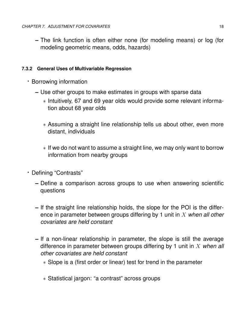
· Borrowing information
– Use other groups to make estimates in groups with sparse data∗ Intuitively, 67 and 69 year olds would provide some relevant informa-
tion about 68 year olds
∗ Assuming a straight line relationship tells us about other, even moredistant, individuals
∗ If we do not want to assume a straight line, we may only want to borrowinformation from nearby groups
· Defining “Contrasts”
– Define a comparison across groups to use when answering scientificquestions
– If the straight line relationship holds, the slope for the POI is the differ-ence in parameter between groups differing by 1 unit in X when all othercovariates are held constant
– If a non-linear relationship in parameter, the slope is still the averagedifference in parameter between groups differing by 1 unit in X when allother covariates are held constant∗ Slope is a (first order or linear) test for trend in the parameter
∗ Statistical jargon: “a contrast” across groups

CHAPTER 7. ADJUSTMENT FOR COVARIATES 19
· The major difference between different regression models is the interpreta-tion of the parameters
– How do I want to summarize the outcome?∗ Mean, geometric mean, odds, hazard
– How do I want to compare groups?∗ Difference, ratio
· Issues related to the inclusion of covariates remains the same
– Address the scientific question: Predictor of interest, effect modification
– Address confounding
– Increase precision
· Interpretation of parameters
– Intercept∗ Corresponds to a population with all modeled covariates equal to zero· Quite often, this will be outside the range of the data so that the
intercept has no meaningful interpretation by itself
– Slope∗ A comparison between groups differing by 1 unit in corresponding co-
variate, but agreeing on all other modeled covariates· Sometimes impossible to use this interpretation when modeling in-
teractions or complex dose-response curves (e.g. a model with ageand age-squared)
· Stratification versus regression
– Generally, any stratified analysis could be performed as a regressionmodel

CHAPTER 7. ADJUSTMENT FOR COVARIATES 20
∗ Stratification adjusts for covariates and all interactions among thosecovariates
∗ Our habit in regression is to just adjust for covariates as main effects,and consider interactions less often
7.3.3 Software
· In Stata or R, we use the same commands as were used for simple regres-sion models
– We just list more variable names
– Interpretations of the CIs, p-values for coefficients estimates now relateto new scientific interpretations of intercept and slopes
– Test of entire regression model also provided (a test that all slopes areequal to zero)
7.3.4 Example: FEV and Smoking
· Scientific question: Is the maximum forced expiatory volume (FEV) relatedto smoking status in children?
· Age ranges from 3 to 19, but no child under 9 smokes in the sample
· Models we will compare
– Unadjusted (simple) model: FEV and smoking
– Adjusted for age: FEV and smoking with age (confounder)
– Adjusted for age, height: FEV and smoking with age (confounder) andheight (precision)

CHAPTER 7. ADJUSTMENT FOR COVARIATES 21
. regress logfev smoker if age>=9, robust
Linear regression Number of obs = 439
F( 1, 437) = 10.45
Prob > F = 0.0013
R-squared = 0.0212
Root MSE = .24765
------------------------------------------------------------------------------
| Robust
logfev | Coef. Std. Err. t P>|t| [95% Conf. Interval]
-------------+----------------------------------------------------------------
smoker | .1023056 .0316539 3.23 0.001 .0400927 .1645184
_cons | 1.05817 .0129335 81.82 0.000 1.032751 1.08359
------------------------------------------------------------------------------
.
. regress logfev smoker age if age>=9, robust
Linear regression Number of obs = 439
F( 2, 436) = 82.28
Prob > F = 0.0000
R-squared = 0.3012
Root MSE = .20949
------------------------------------------------------------------------------
| Robust
logfev | Coef. Std. Err. t P>|t| [95% Conf. Interval]
-------------+----------------------------------------------------------------
smoker | -.0513495 .0343822 -1.49 0.136 -.118925 .016226
age | .0635957 .0051401 12.37 0.000 .0534932 .0736981
_cons | .3518165 .0575011 6.12 0.000 .2388028 .4648303
------------------------------------------------------------------------------
.
. regress logfev smoker age loght if age >=9, robust
Linear regression Number of obs = 439
F( 3, 435) = 284.22
Prob > F = 0.0000
R-squared = 0.6703
Root MSE = .14407
------------------------------------------------------------------------------
| Robust
logfev | Coef. Std. Err. t P>|t| [95% Conf. Interval]
-------------+----------------------------------------------------------------
smoker | -.0535896 .0241879 -2.22 0.027 -.1011293 -.00605
age | .0215295 .0034817 6.18 0.000 .0146864 .0283725
loght | 2.869658 .1279943 22.42 0.000 2.618093 3.121222
_cons | -11.09461 .5153323 -21.53 0.000 -12.10746 -10.08176
------------------------------------------------------------------------------
CHAPTER 7. ADJUSTMENT FOR COVARIATES 22
7.4 Unadjusted versus Adjusted Models
7.4.1 General comparison
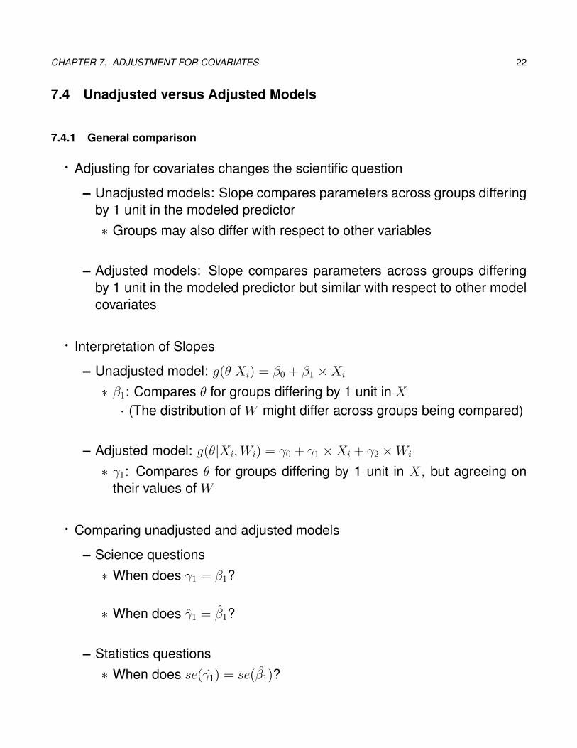
· Adjusting for covariates changes the scientific question
– Unadjusted models: Slope compares parameters across groups differingby 1 unit in the modeled predictor∗ Groups may also differ with respect to other variables
– Adjusted models: Slope compares parameters across groups differingby 1 unit in the modeled predictor but similar with respect to other modelcovariates
· Interpretation of Slopes
– Unadjusted model: g(θ|Xi) = β0 + β1 ×Xi
∗ β1: Compares θ for groups differing by 1 unit in X· (The distribution of W might differ across groups being compared)
– Adjusted model: g(θ|Xi,Wi) = γ0 + γ1 ×Xi + γ2 ×Wi
∗ γ1: Compares θ for groups differing by 1 unit in X, but agreeing ontheir values of W
· Comparing unadjusted and adjusted models
– Science questions∗ When does γ1 = β1?
∗ When does γ1 = β1?
– Statistics questions∗ When does se(γ1) = se(β1)?

CHAPTER 7. ADJUSTMENT FOR COVARIATES 23
∗ When does se(γ1) = se(β1)
– In above, note placement of theˆ(“hat”) which signifies estimates of pop-ulation parameters
– Lack of a hat indicates “the truth” in the population
– When γ1 = β1 (the formulas are the same), then it must be the case thatse(γ1) = se(β1)
∗ But our estimates of the standard errors may not be the same
– Example of when γ1 = β1
∗ Want to compare smokers to non-smokers (POI) with respect to theirFEV (response) and have conducted a randomized experiment in whichboys and girls (W ) are equally represented as smokers and non-smokers
∗ When we compare a random smoker to a random non-smoker, thataverage difference will be the same if we adjust for gender or not
∗ Numbers in unadjusted and adjusted analyses are the same, but in-terpretation is different
· Answering these four questions cannot be done in the general case
– However, in linear regression we can derive exact results
– These exact results can serve as a basis for examination of other regres-sion models∗ Logistic regression
∗ Poisson regression

CHAPTER 7. ADJUSTMENT FOR COVARIATES 24
∗ Proportional hazards regression
7.4.2 Comparison of Adjusted and Unadjusted Models in Linear Regression
Interpretation of Slopes
· Unadjusted model: E[Yi|Xi] = β0 + β1 ×Xi
– β1: Difference in mean Y for groups differing by 1 unit in X∗ (The distribution of W might differ across groups being compared)
· Adjusted model: E[Yi|Xi,Wi] = γ0 + γ1 ×Xi + γ2 ×Wi
– γ1: Difference in mean Y for groups differing by 1 unit in X, but agreeingin their values of W
Relationships: True Slopes
· The slope of the unadjusted model will tend to be
β1 = γ1 + ρXWσWσX
γ2 (7.5)
· Hence, true adjusted and unadjusted slopes for X are estimating the samequantity on if
– ρXW = 0 (X and W are truly uncorrelated), OR
– γ2 = 0 (no association between W and Y after adjusting for X)
Relationships: Estimated Slopes
· The estimated slope of the unadjusted model will be
CHAPTER 7. ADJUSTMENT FOR COVARIATES 25
β1 = γ1
1 + γ2rXW
sWsX(rY X − rYWrXW
(7.6)
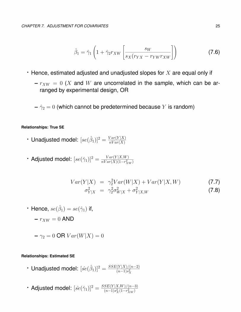
· Hence, estimated adjusted and unadjusted slopes for X are equal only if
– rXW = 0 (X and W are uncorrelated in the sample, which can be ar-ranged by experimental design, OR
– γ2 = 0 (which cannot be predetermined because Y is random)
Relationships: True SE
· Unadjusted model: [se(β1)]2 = V ar(Y |X)nV ar(X)
· Adjusted model: [se(γ1)]2 = V ar(Y |X,W )nV ar(X)(1−r2XW )
V ar(Y |X) = γ22V ar(W |X) + V ar(Y |X,W ) (7.7)σ2Y |X = γ22σ
2W |X + σ2Y |X,W (7.8)
· Hence, se(β1) = se(γ1) if,
– rXW = 0 AND
– γ2 = 0 OR V ar(W |X) = 0
Relationships: Estimated SE
· Unadjusted model: [se(β1)]2 = SSE(Y |X)/(n−2)(n−1)s2X
· Adjusted model: [se(γ1)]2 = SSE(Y |X,W )/(n−3)(n−1)s2X(1−r2XW )
CHAPTER 7. ADJUSTMENT FOR COVARIATES 26
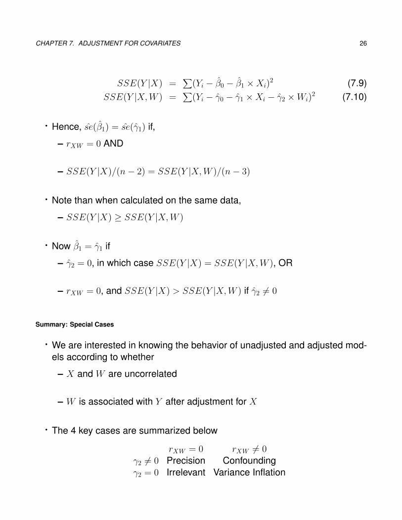
SSE(Y |X) =∑
(Yi − β0 − β1 ×Xi)2 (7.9)
SSE(Y |X,W ) =∑
(Yi − γ0 − γ1 ×Xi − γ2 ×Wi)2 (7.10)
· Hence, se(β1) = se(γ1) if,
– rXW = 0 AND
– SSE(Y |X)/(n− 2) = SSE(Y |X,W )/(n− 3)
· Note than when calculated on the same data,
– SSE(Y |X) ≥ SSE(Y |X,W )
· Now β1 = γ1 if
– γ2 = 0, in which case SSE(Y |X) = SSE(Y |X,W ), OR
– rXW = 0, and SSE(Y |X) > SSE(Y |X,W ) if γ2 6= 0
Summary: Special Cases
· We are interested in knowing the behavior of unadjusted and adjusted mod-els according to whether
– X and W are uncorrelated
– W is associated with Y after adjustment for X
· The 4 key cases are summarized below
rXW = 0 rXW 6= 0γ2 6= 0 Precision Confoundingγ2 = 0 Irrelevant Variance Inflation
CHAPTER 7. ADJUSTMENT FOR COVARIATES 27
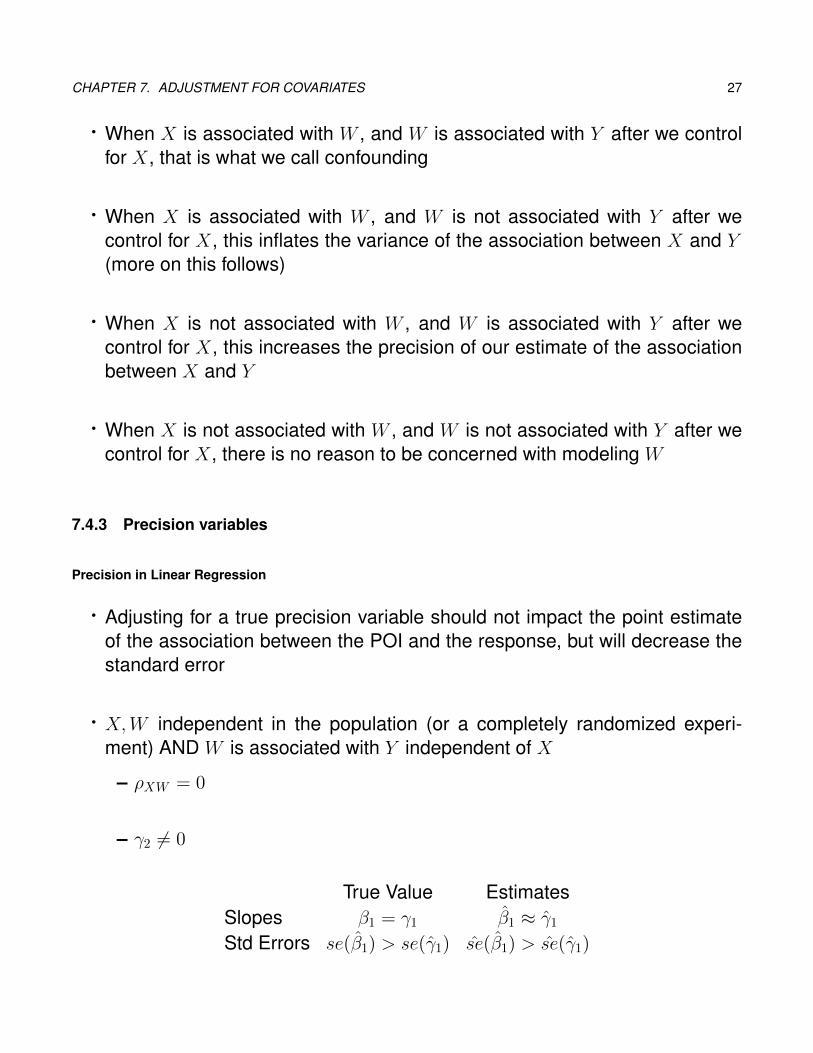
· When X is associated with W , and W is associated with Y after we controlfor X, that is what we call confounding
· When X is associated with W , and W is not associated with Y after wecontrol for X, this inflates the variance of the association between X and Y(more on this follows)
· When X is not associated with W , and W is associated with Y after wecontrol for X, this increases the precision of our estimate of the associationbetween X and Y
· When X is not associated with W , and W is not associated with Y after wecontrol for X, there is no reason to be concerned with modeling W
7.4.3 Precision variables
Precision in Linear Regression
· Adjusting for a true precision variable should not impact the point estimateof the association between the POI and the response, but will decrease thestandard error
· X,W independent in the population (or a completely randomized experi-ment) AND W is associated with Y independent of X
– ρXW = 0
– γ2 6= 0
True Value EstimatesSlopes β1 = γ1 β1 ≈ γ1Std Errors se(β1) > se(γ1) se(β1) > se(γ1)
CHAPTER 7. ADJUSTMENT FOR COVARIATES 28
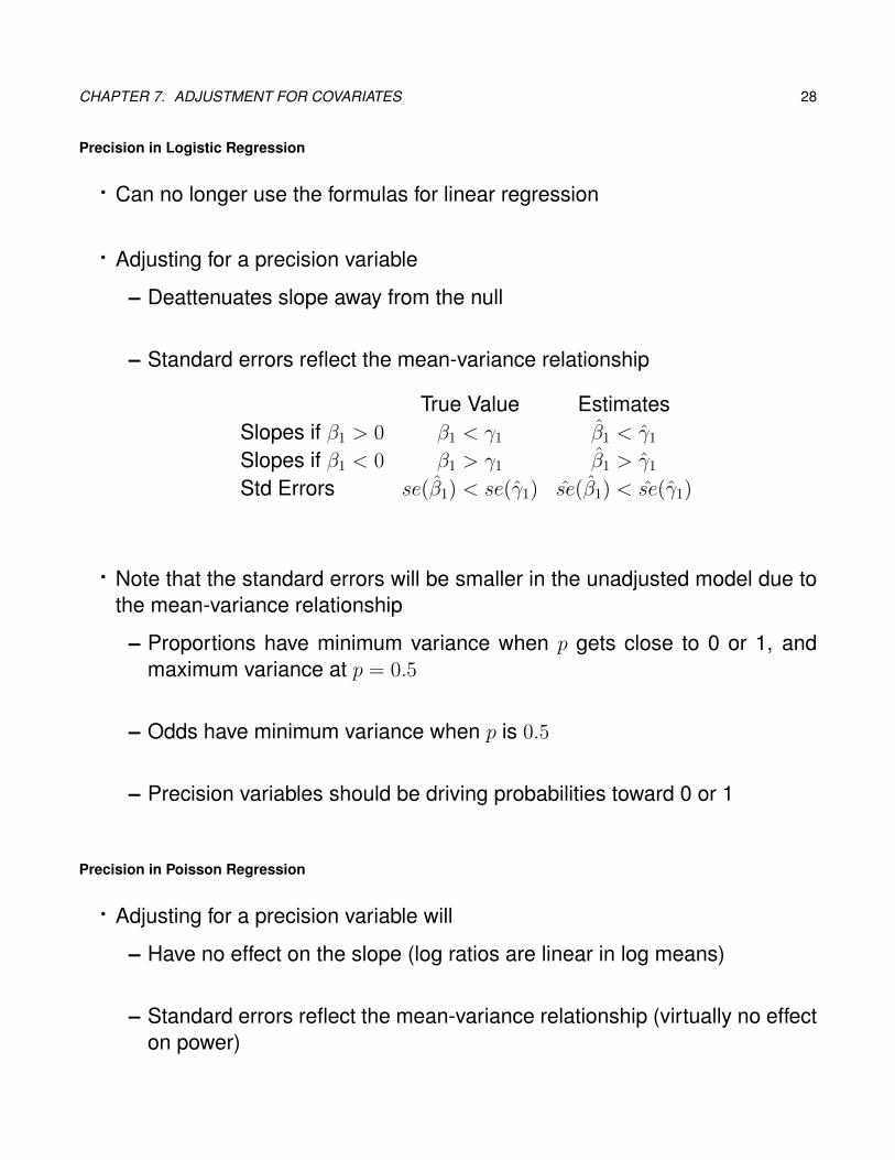
Precision in Logistic Regression
· Can no longer use the formulas for linear regression
· Adjusting for a precision variable
– Deattenuates slope away from the null
– Standard errors reflect the mean-variance relationship
True Value EstimatesSlopes if β1 > 0 β1 < γ1 β1 < γ1Slopes if β1 < 0 β1 > γ1 β1 > γ1Std Errors se(β1) < se(γ1) se(β1) < se(γ1)
· Note that the standard errors will be smaller in the unadjusted model due tothe mean-variance relationship
– Proportions have minimum variance when p gets close to 0 or 1, andmaximum variance at p = 0.5
– Odds have minimum variance when p is 0.5
– Precision variables should be driving probabilities toward 0 or 1
Precision in Poisson Regression
· Adjusting for a precision variable will
– Have no effect on the slope (log ratios are linear in log means)
– Standard errors reflect the mean-variance relationship (virtually no effecton power)
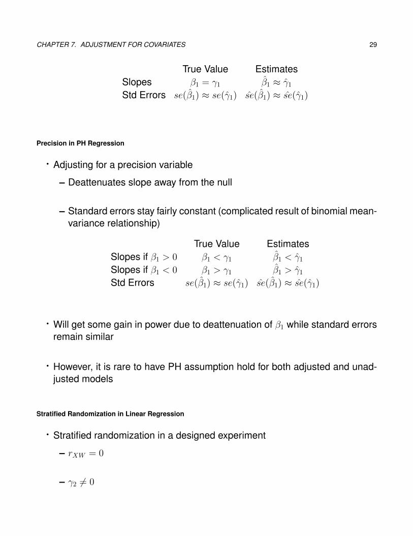
CHAPTER 7. ADJUSTMENT FOR COVARIATES 29
True Value EstimatesSlopes β1 = γ1 β1 ≈ γ1Std Errors se(β1) ≈ se(γ1) se(β1) ≈ se(γ1)
Precision in PH Regression
· Adjusting for a precision variable
– Deattenuates slope away from the null
– Standard errors stay fairly constant (complicated result of binomial mean-variance relationship)
True Value EstimatesSlopes if β1 > 0 β1 < γ1 β1 < γ1Slopes if β1 < 0 β1 > γ1 β1 > γ1Std Errors se(β1) ≈ se(γ1) se(β1) ≈ se(γ1)
· Will get some gain in power due to deattenuation of β1 while standard errorsremain similar
· However, it is rare to have PH assumption hold for both adjusted and unad-justed models
Stratified Randomization in Linear Regression
· Stratified randomization in a designed experiment
– rXW = 0
– γ2 6= 0
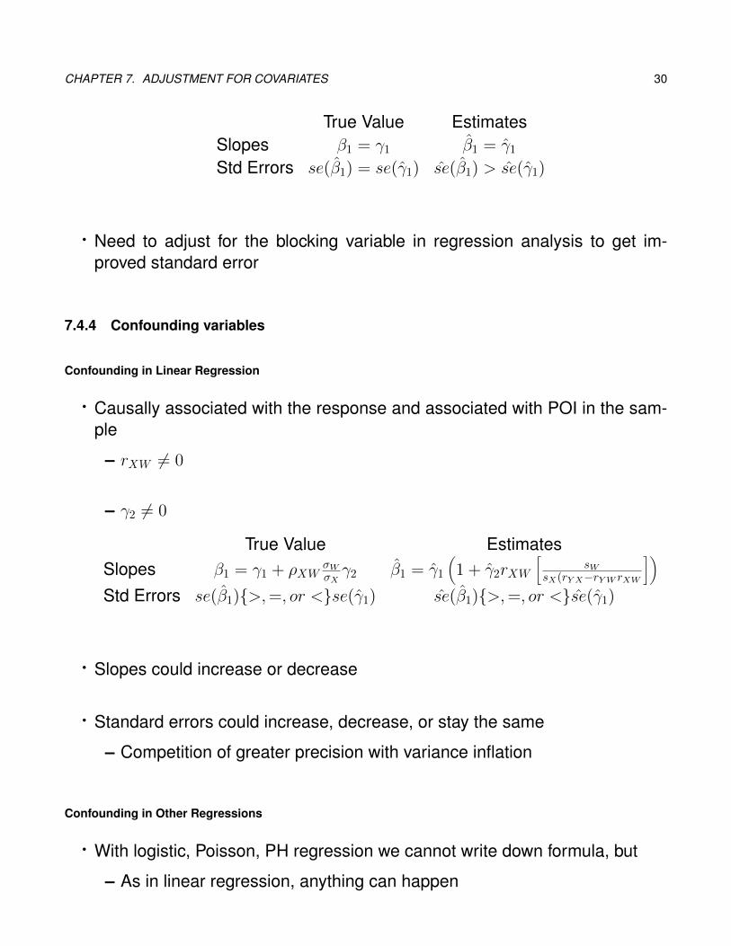
CHAPTER 7. ADJUSTMENT FOR COVARIATES 30
True Value EstimatesSlopes β1 = γ1 β1 = γ1Std Errors se(β1) = se(γ1) se(β1) > se(γ1)
· Need to adjust for the blocking variable in regression analysis to get im-proved standard error
7.4.4 Confounding variables
Confounding in Linear Regression
· Causally associated with the response and associated with POI in the sam-ple
– rXW 6= 0
– γ2 6= 0
True Value EstimatesSlopes β1 = γ1 + ρXW
σWσXγ2 β1 = γ1
(1 + γ2rXW
[sW
sX(rY X−rYW rXW
])Std Errors se(β1){>,=, or <}se(γ1) se(β1){>,=, or <}se(γ1)
· Slopes could increase or decrease
· Standard errors could increase, decrease, or stay the same
– Competition of greater precision with variance inflation
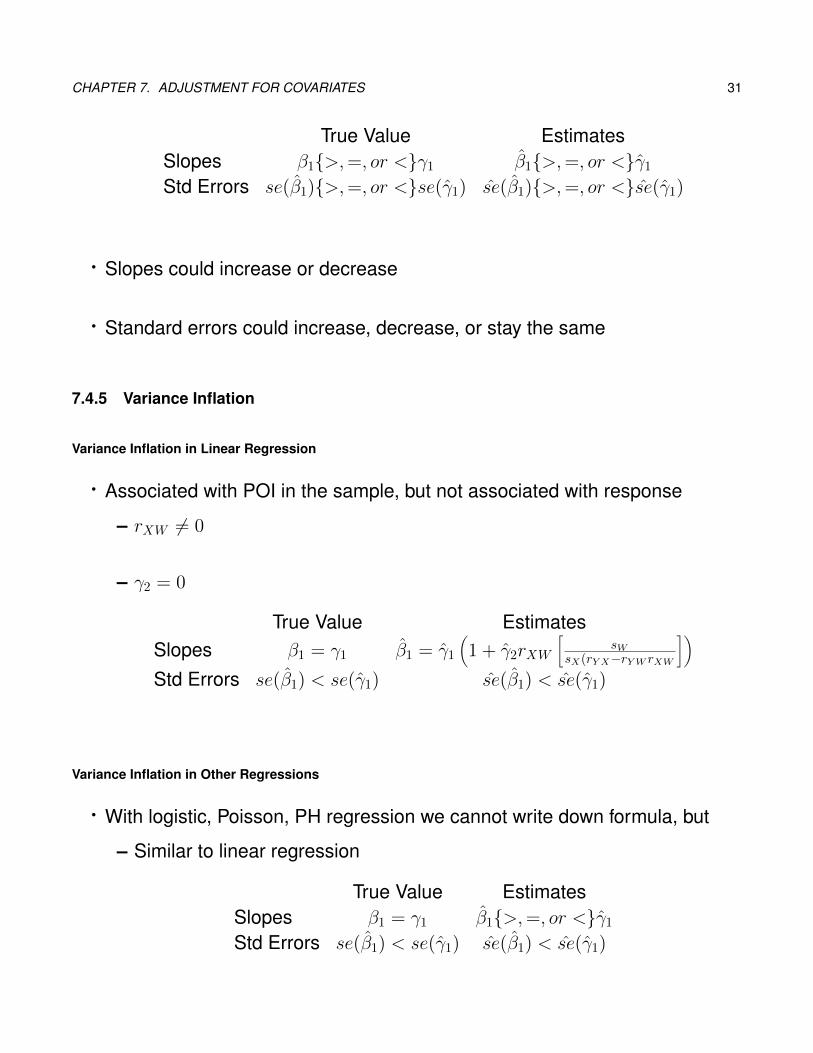
Confounding in Other Regressions
· With logistic, Poisson, PH regression we cannot write down formula, but
– As in linear regression, anything can happen
CHAPTER 7. ADJUSTMENT FOR COVARIATES 31
True Value EstimatesSlopes β1{>,=, or <}γ1 β1{>,=, or <}γ1Std Errors se(β1){>,=, or <}se(γ1) se(β1){>,=, or <}se(γ1)
· Slopes could increase or decrease
· Standard errors could increase, decrease, or stay the same
7.4.5 Variance Inflation
Variance Inflation in Linear Regression
· Associated with POI in the sample, but not associated with response
– rXW 6= 0
– γ2 = 0
True Value EstimatesSlopes β1 = γ1 β1 = γ1
(1 + γ2rXW
[sW
sX(rY X−rYW rXW
])Std Errors se(β1) < se(γ1) se(β1) < se(γ1)
Variance Inflation in Other Regressions
· With logistic, Poisson, PH regression we cannot write down formula, but
– Similar to linear regression
True Value EstimatesSlopes β1 = γ1 β1{>,=, or <}γ1Std Errors se(β1) < se(γ1) se(β1) < se(γ1)
CHAPTER 7. ADJUSTMENT FOR COVARIATES 32
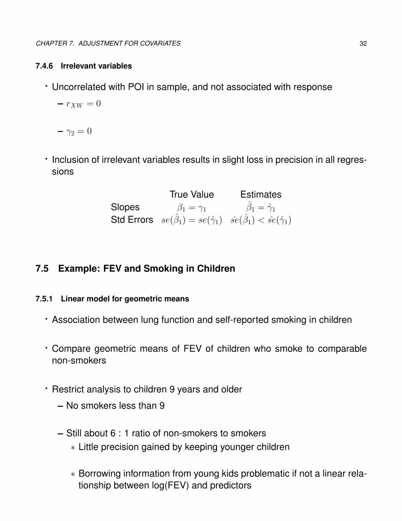
7.4.6 Irrelevant variables
· Uncorrelated with POI in sample, and not associated with response
– rXW = 0
– γ2 = 0
· Inclusion of irrelevant variables results in slight loss in precision in all regres-sions
True Value EstimatesSlopes β1 = γ1 β1 = γ1Std Errors se(β1) = se(γ1) se(β1) < se(γ1)
7.5 Example: FEV and Smoking in Children
7.5.1 Linear model for geometric means
· Association between lung function and self-reported smoking in children
· Compare geometric means of FEV of children who smoke to comparablenon-smokers
· Restrict analysis to children 9 years and older
– No smokers less than 9
– Still about 6 : 1 ratio of non-smokers to smokers∗ Little precision gained by keeping younger children
∗ Borrowing information from young kids problematic if not a linear rela-tionship between log(FEV) and predictors
CHAPTER 7. ADJUSTMENT FOR COVARIATES 33
∗ With confounding, want to get the model correct
· Academic Exercise: Compare alternative models
– In real life, we should choose a single model in advance of looking at thedata
– Here we will observe what happens to parameter estimates and SEacross models∗ Smoking
∗ Smoking adjusted for age
∗ Smoking adjusted for age and height
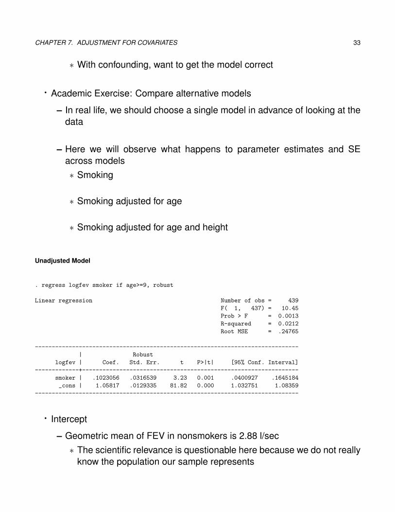
Unadjusted Model
. regress logfev smoker if age>=9, robust
Linear regression Number of obs = 439
F( 1, 437) = 10.45
Prob > F = 0.0013
R-squared = 0.0212
Root MSE = .24765
------------------------------------------------------------------------------
| Robust
logfev | Coef. Std. Err. t P>|t| [95% Conf. Interval]
-------------+----------------------------------------------------------------
smoker | .1023056 .0316539 3.23 0.001 .0400927 .1645184
_cons | 1.05817 .0129335 81.82 0.000 1.032751 1.08359
------------------------------------------------------------------------------
· Intercept
– Geometric mean of FEV in nonsmokers is 2.88 l/sec∗ The scientific relevance is questionable here because we do not really
know the population our sample represents

CHAPTER 7. ADJUSTMENT FOR COVARIATES 34
∗ Calculations e1.05817 = 2.88
∗ The p-value is completely unimportant here as it is testing that the loggeometric mean is 0, or that the geometric mean is 1. Why would wecare?
– Because smoker is a binary variable, the estimate corresponds to a ge-ometric mean. In many regression models, the intercept will have notinterpretation
· Smoking effect
– Geometric mean of FEV is 10.8% higher in smokers than in nonsmokers(95% CI: 4.1% to 17.9% higher)∗ These results are atypical of what we might expect with no true differ-
ence between groups (p = 0.001)
∗ Calculations: e.102 = 1.108; e.040 = 1.041; e0.165 = 1.179
∗ (Note that ex is approximately (1 + x) for x close to 1)
– Because smoker is a binary variable, this analysis is nearly identical to atwo sample t-test allowing for unequal variances
CHAPTER 7. ADJUSTMENT FOR COVARIATES 35
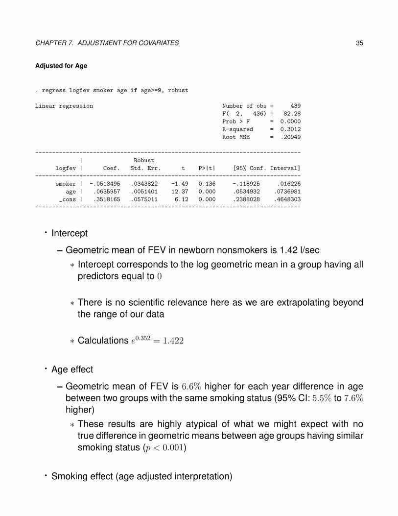
Adjusted for Age
. regress logfev smoker age if age>=9, robust
Linear regression Number of obs = 439
F( 2, 436) = 82.28
Prob > F = 0.0000
R-squared = 0.3012
Root MSE = .20949
------------------------------------------------------------------------------
| Robust
logfev | Coef. Std. Err. t P>|t| [95% Conf. Interval]
-------------+----------------------------------------------------------------
smoker | -.0513495 .0343822 -1.49 0.136 -.118925 .016226
age | .0635957 .0051401 12.37 0.000 .0534932 .0736981
_cons | .3518165 .0575011 6.12 0.000 .2388028 .4648303
------------------------------------------------------------------------------
· Intercept
– Geometric mean of FEV in newborn nonsmokers is 1.42 l/sec∗ Intercept corresponds to the log geometric mean in a group having all
predictors equal to 0
∗ There is no scientific relevance here as we are extrapolating beyondthe range of our data
∗ Calculations e0.352 = 1.422
· Age effect
– Geometric mean of FEV is 6.6% higher for each year difference in agebetween two groups with the same smoking status (95% CI: 5.5% to 7.6%higher)∗ These results are highly atypical of what we might expect with no
true difference in geometric means between age groups having similarsmoking status (p < 0.001)
· Smoking effect (age adjusted interpretation)

CHAPTER 7. ADJUSTMENT FOR COVARIATES 36
– Geometric mean of FEV is 5.0% lower in smokers than in nonsmokers ofthe same age (95% CI: 12.2% lower to 1.6% higher)∗ These results are not atypical of what we might expect with no true
difference between groups of the same age (p = 0.136)
∗ Lack of statistical significance can also be noted by the fact that theCI for the ratio contain 1 or the CI for the percent difference contains0
∗ Calculations: e−.051 = 0.950; e−.119 = 0.888; e0.016 = 1.016
· Comparing unadjusted and age adjusted analyses
– Marked differences in effect of smoking suggests that there was indeedconfounding∗ Age is a relatively strong predictor of FEV
∗ Age is associated with smoking in the sample· Mean (SD) of age in analyzed smokers: 11.1 (2.04)
· Mean (SD) of age in analyzed nonsmokers: 13.5 (2.34)
– Effect of age adjustment on precision∗ Lower Root MSE (0.209 vs 0.248) would tend to increase precision of
estimate of smoking effect
∗ Association between smoking and age tends to lower precision
∗ Net effect: Less precision (adj SE 0.034 vs unadj SE 0.031)
CHAPTER 7. ADJUSTMENT FOR COVARIATES 37
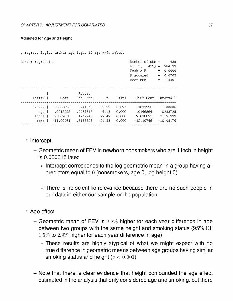
Adjusted for Age and Height
. regress logfev smoker age loght if age >=9, robust
Linear regression Number of obs = 439
F( 3, 435) = 284.22
Prob > F = 0.0000
R-squared = 0.6703
Root MSE = .14407
------------------------------------------------------------------------------
| Robust
logfev | Coef. Std. Err. t P>|t| [95% Conf. Interval]
-------------+----------------------------------------------------------------
smoker | -.0535896 .0241879 -2.22 0.027 -.1011293 -.00605
age | .0215295 .0034817 6.18 0.000 .0146864 .0283725
loght | 2.869658 .1279943 22.42 0.000 2.618093 3.121222
_cons | -11.09461 .5153323 -21.53 0.000 -12.10746 -10.08176
------------------------------------------------------------------------------
· Intercept
– Geometric mean of FEV in newborn nonsmokers who are 1 inch in heightis 0.000015 l/sec∗ Intercept corresponds to the log geometric mean in a group having all
predictors equal to 0 (nonsmokers, age 0, log height 0)
∗ There is no scientific relevance because there are no such people inour data in either our sample or the population
· Age effect
– Geometric mean of FEV is 2.2% higher for each year difference in agebetween two groups with the same height and smoking status (95% CI:1.5% to 2.9% higher for each year difference in age)∗ These results are highly atypical of what we might expect with no
true difference in geometric means between age groups having similarsmoking status and height (p < 0.001)
– Note that there is clear evidence that height confounded the age effectestimated in the analysis that only considered age and smoking, but there

CHAPTER 7. ADJUSTMENT FOR COVARIATES 38
is still a clearly independent effect of age on FEV
· Height effect
– Geometric mean of FEV is 31.5% higher for each 10% difference in heightbetween two groups with the same age and smoking status (95% CI:28.3% to 34.6% higher for each 10% difference in height)∗ These results are highly atypical of what we might expect with no true
difference in geometric means between height groups having similarsmoking status and age (p < 0.001)
∗ Calculations: 1.12.867 = 1.315
– Note that the CI for the regression coefficient is consistent with the scientifically-hypothesize value of 3
· Smoking effect (age, height adjusted interpretation)
– Geometric mean of FEV is 5.2% lower in smokers than in nonsmokers ofthe same age and height (95% CI: 9.6% to 0.6% lower)∗ These results are atypical of what we might expect with no true differ-
ence between groups of the same age and height (p = 0.027)
∗ Calculations: e−.054 = 0.948; e−.101 = 0.904; e−0.006 = .994
· Comparing age-adjusted to age- and height-adjusted analyses
– No difference in effect of smoking suggests that there was no more con-founding after age adjustment
– Effect of height adjustment on precision∗ Lower Root MSE (0.144 vs 0.209) would tend to increase precision of
estimate of smoking effect

CHAPTER 7. ADJUSTMENT FOR COVARIATES 39
∗ Little association between smoking and height after adjusting for agewill not tend to lower precision
∗ Net effect: Higher precision (adj SE 0.024 vs unadj SE 0.034)
7.5.2 Logistic model
· Continue our academic exercise using logistic regression
– Dichotomize FEV at median (2.93)
– In real life, we would not want to make a continuous variable like FEV intoa binary variable
– Here we will observe what happens to parameter estimates and SEacross models∗ Smoking
∗ Smoking adjusted for age
∗ Smoking adjusted for height
∗ Smoking adjusted for age and height

CHAPTER 7. ADJUSTMENT FOR COVARIATES 40
. logit fevbin smoker if age>=9
Logistic regression Number of obs = 439
LR chi2(1) = 15.81
Prob > chi2 = 0.0001
Log likelihood = -296.38409 Pseudo R2 = 0.0260
------------------------------------------------------------------------------
fevbin | Coef. Std. Err. z P>|z| [95% Conf. Interval]
-------------+----------------------------------------------------------------
smoker | 1.120549 .2959672 3.79 0.000 .540464 1.700634
_cons | -.1607732 .1037519 -1.55 0.121 -.3641231 .0425767
------------------------------------------------------------------------------
.
. logit fevbin smoker age if age>=9
Logistic regression Number of obs = 439
LR chi2(2) = 88.68
Prob > chi2 = 0.0000
Log likelihood = -259.95032 Pseudo R2 = 0.1457
------------------------------------------------------------------------------
fevbin | Coef. Std. Err. z P>|z| [95% Conf. Interval]
-------------+----------------------------------------------------------------
smoker | .1971403 .3402482 0.58 0.562 -.469734 .8640146
age | .470792 .0637495 7.39 0.000 .3458453 .5957386
_cons | -5.360912 .7056265 -7.60 0.000 -6.743914 -3.977909
------------------------------------------------------------------------------
.
. logit fevbin smoker loght if age>=9
Logistic regression Number of obs = 439
LR chi2(2) = 224.11
Prob > chi2 = 0.0000
Log likelihood = -192.23646 Pseudo R2 = 0.3682
------------------------------------------------------------------------------
fevbin | Coef. Std. Err. z P>|z| [95% Conf. Interval]
-------------+----------------------------------------------------------------
smoker | .4159311 .3646506 1.14 0.254 -.2987709 1.130633
loght | 33.08872 3.169516 10.44 0.000 26.87659 39.30086
_cons | -137.6043 13.16723 -10.45 0.000 -163.4116 -111.797
------------------------------------------------------------------------------
.
. logit fevbin smoker age loght if age>=9
Logistic regression Number of obs = 439
LR chi2(3) = 230.19
Prob > chi2 = 0.0000
Log likelihood = -189.19487 Pseudo R2 = 0.3782
------------------------------------------------------------------------------
fevbin | Coef. Std. Err. z P>|z| [95% Conf. Interval]
-------------+----------------------------------------------------------------
smoker | .047695 .3933191 0.12 0.903 -.7231963 .8185863
age | .1753759 .0723176 2.43 0.015 .033636 .3171157
loght | 31.04791 3.289031 9.44 0.000 24.60152 37.49429
_cons | -131.0647 13.5393 -9.68 0.000 -157.6013 -104.5282
------------------------------------------------------------------------------

CHAPTER 7. ADJUSTMENT FOR COVARIATES 41
Results Summarized
· Coefficients (logit scale)
Model Smoker Age Log(Height)Smoke 1.12Smoke+Age 0.19 0.47Smoke+Ht 0.42 33.1Smoke+Age+Ht 0.47 0.18 31.0
· Std Errors (logit scale)
Model Smoker Age Log(Height)Smoke 0.30Smoke+Age 0.34 0.06Smoke+Ht 0.36 3.2Smoke+Age+Ht 0.39 0.07 3.3
· Adjusting for the height
– Comparing Smoke+Age to Smoke+Age+Ht∗ Height is being added as a precision variable
∗ Deattenuated the smoking effect (estimate changes from 0.19 to 0.47,which is further from 0)
∗ Increased the standard error estimate (0.34 to 0.39)
∗ Both of these change are predicted by the previous discusssion
– Comparing Smoke to Smoke+Ht∗ Attenuated the smoking effect (1.12 to 0.42, closer to 0)
∗ Increased the standard error estimate

CHAPTER 7. ADJUSTMENT FOR COVARIATES 42
∗ Height now also acting acting as a confounding variable (because weare not modeling age), so these changes were not predictable
· Adjusting for the confounding variable (age)
– Comparing Smoke+Ht to Smoke+Age+Ht∗ Deattenuated the estimated coefficient (0.42 to 0.47)
∗ Increased the standard error
– Comparing Smoke to Smoke+Age∗ Attenuated the coefficient estimate (1.12 to 0.19)
∗ Increased the standard error
– Changes in estimates and standard errors were not predictable for this,or any, confounder