Biopac Student Lab 4.1 BSL PRO TUTORIAL · 2 Biopac Student Lab Welcome to the Biopac Student Lab...

Biopac Student Lab 4.1

Windows 10, 8, 7

Mac OS 10.10-10.14

BSL PRO TUTORIAL

BIOPAC Systems, Inc. 42 Aero Camino, Goleta, CA 93117

(805) 685-0066, Fax (805) 685-0067

[email protected]

www.biopac.com

04.28.19

mailto:[email protected]

2 Biopac Student Lab

Welcome to the Biopac Student Lab PRO!

To learn how the Biopac Student Lab PRO works, complete this interactive Tutorial and read the Overview Chapter of

the BSL PRO Manual. For an in-depth discussion of BSL PRO features and how they can make your work easier, read

further chapters of the BSL PRO Manual.

The BSL PRO Manual (PDF format) is under the Help menu of the BSL PRO application.

Note that it is not necessary to record data (nor be connected to the MP recording hardware) to conduct this tutorial.

The particulars of setup and recording are application specific and are discussed only generally in this Tutorial. For

detailed instructions about setup and recording, consult the BSL PRO Manual and the BSL PRO Hardware Guide—and

follow your particular lesson plans and application notes.

This tutorial demonstrates use of BSL PRO software using BIOPAC MP36 or MP35 data acquisition units. MP45 users may note different features when using the software —consult the BSL PRO Manual for more detailed

information about using BSL PRO with all MP hardware. (MP30 hardware is not supported in BSL PRO 4.)

All life science applications for the BSL PRO system involve setting up the hardware for acquiring signals (such as

electrodes, leads, and the BIOPAC MP data acquisition unit,) setting up BSL PRO software, acquiring data (recording)

and analyzing the data.

This tutorial assumes BSL PRO is already installed to your hard drive. (If not, insert the CD and follow the prompts.)

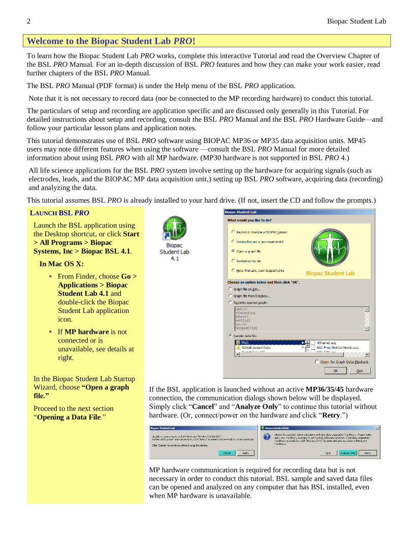
LAUNCH BSL PRO

Launch the BSL application using

the Desktop shortcut, or click Start

> All Programs > Biopac

Systems, Inc > Biopac BSL 4.1.

In Mac OS X:

▪ From Finder, choose Go >

Applications > Biopac

Student Lab 4.1 and

double-click the Biopac

Student Lab application

icon.

▪ If MP hardware is not

connected or is

unavailable, see details at

right.

In the Biopac Student Lab Startup Wizard, choose “Open a graph

file.”

Proceed to the next section

“Opening a Data File.”

If the BSL application is launched without an active MP36/35/45 hardware

connection, the communication dialogs shown below will be displayed.

Simply click “Cancel” and “Analyze Only” to continue this tutorial without

hardware. (Or, connect/power on the hardware and click “Retry.”)

MP hardware communication is required for recording data but is not

necessary in order to conduct this tutorial. BSL sample and saved data files can be opened and analyzed on any computer that has BSL installed, even

when MP hardware is unavailable.

BSL PRO Tutorial 3

© BIOPAC Systems, Inc. www.biopac.com

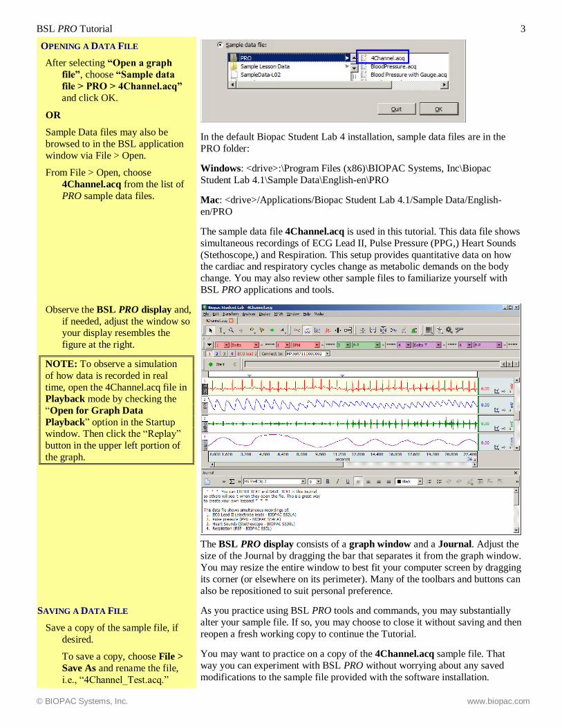
OPENING A DATA FILE

After selecting “Open a graph

file”, choose “Sample data

file > PRO > 4Channel.acq”

and click OK.

OR

Sample Data files may also be

browsed to in the BSL application

window via File > Open.

From File > Open, choose

4Channel.acq from the list of

PRO sample data files.

In the default Biopac Student Lab 4 installation, sample data files are in the

PRO folder:

Windows: <drive>:\Program Files (x86)\BIOPAC Systems, Inc\Biopac

Student Lab 4.1\Sample Data\English-en\PRO

Mac: <drive>/Applications/Biopac Student Lab 4.1/Sample Data/English-

en/PRO

The sample data file 4Channel.acq is used in this tutorial. This data file shows

simultaneous recordings of ECG Lead II, Pulse Pressure (PPG,) Heart Sounds

(Stethoscope,) and Respiration. This setup provides quantitative data on how the cardiac and respiratory cycles change as metabolic demands on the body

change. You may also review other sample files to familiarize yourself with

BSL PRO applications and tools.

Observe the BSL PRO display and,

if needed, adjust the window so your display resembles the

figure at the right.

NOTE: To observe a simulation

of how data is recorded in real

time, open the 4Channel.acq file in Playback mode by checking the

“Open for Graph Data

Playback” option in the Startup window. Then click the “Replay”

button in the upper left portion of

the graph.

The BSL PRO display consists of a graph window and a Journal. Adjust the

size of the Journal by dragging the bar that separates it from the graph window.

You may resize the entire window to best fit your computer screen by dragging

its corner (or elsewhere on its perimeter). Many of the toolbars and buttons can

also be repositioned to suit personal preference.

SAVING A DATA FILE

Save a copy of the sample file, if

desired.

To save a copy, choose File >

Save As and rename the file,

i.e., “4Channel_Test.acq.”

As you practice using BSL PRO tools and commands, you may substantially

alter your sample file. If so, you may choose to close it without saving and then

reopen a fresh working copy to continue the Tutorial.

You may want to practice on a copy of the 4Channel.acq sample file. That

way you can experiment with BSL PRO without worrying about any saved

modifications to the sample file provided with the software installation.


By default, BSL PRO data files are saved in the BSL PRO format with the

“.acq” filename extension. Saving a file in the BSL PRO format saves the graph data and the journal notes, the setup parameters (established under the

MP menu,) and window positions. Except in exceptional cases, you will save

data files in the default graph (*.acq) or graph template (*.gtl) format.

IMPORTANT! Saving as a Graph Template does not save any data—only

the setup parameters.

Part 1: Acquisition

Parameters

Each BSL PRO lesson—including experiments that you may design—will

have unique procedures for attaching electrodes, transducers, and other signal

monitoring equipment. Signal monitoring equipment is connected to the MP

hardware, and the MP hardware in turn is connected to the computer. Follow

the instructions for your particular experiment to set up the hardware.

Before recording, however, you must set data acquisition parameters in the

BSL PRO software. (See “Set Up Acquisition” on page 10 and “Part 2:

Recording” on page 11 for more details. Again, it is not necessary to record

data in order to conduct this tutorial.)

SET UP CHANNELS

Choose the menu command

MP menu > Set Up Data

Acquisition > Channels to

generate the Data Acquisition

Settings dialog.

The Data Acquisition Settings dialog displays options for determining which

channels receive data, what type of data the channels receive, and how data is

displayed and interpreted onscreen.

Data Input Channels

Analog Channels

Digital Channels

Calculation Channels

Note the three kinds of data input

channels and read about them

at right.

Analog Channels (above) are the most common type of channel and are used

to acquire any data with “continuous” values. Examples of this include nearly all physiological applications where input devices (transducers and electrodes)

produce a continuous stream of varying data.

• BSL PRO records and displays up to four analog signals from devices

connected to analog input ports on the front panel of the MP unit.

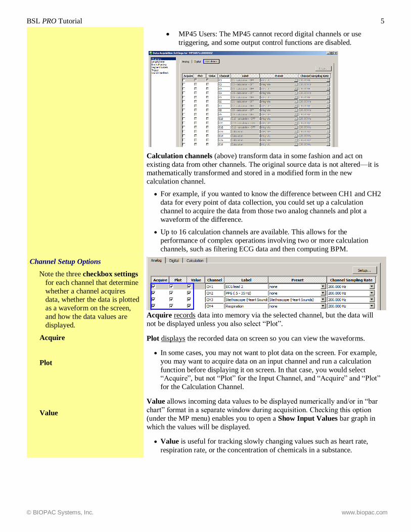
Digital Channels (above) in contrast to analog input channels, collect data

from signal sources operating with only two values, such as on/off devices.

Digital channels are used, for example, in studies of stimulus response patterns

and reaction time to log signals from push-button switches, auditory/visual

stimulus devices, and timing devices.

• BSL PRO records and displays up to eight digital signals from

devices connected to the I/O port on the back of the MP unit.

BSL PRO Tutorial 5


• MP45 Users: The MP45 cannot record digital channels or use

triggering, and some output control functions are disabled.

Calculation channels (above) transform data in some fashion and act on

existing data from other channels. The original source data is not altered—it is mathematically transformed and stored in a modified form in the new

calculation channel.

• For example, if you wanted to know the difference between CH1 and CH2

data for every point of data collection, you could set up a calculation

channel to acquire the data from those two analog channels and plot a

waveform of the difference.

• Up to 16 calculation channels are available. This allows for the

performance of complex operations involving two or more calculation

channels, such as filtering ECG data and then computing BPM.

Channel Setup Options

Note the three checkbox settings

for each channel that determine

whether a channel acquires data, whether the data is plotted

as a waveform on the screen,

and how the data values are

displayed.

Acquire

Plot

Value

Acquire records data into memory via the selected channel, but the data will

not be displayed unless you also select “Plot”.

Plot displays the recorded data on screen so you can view the waveforms.

• In some cases, you may not want to plot data on the screen. For example,

you may want to acquire data on an input channel and run a calculation

function before displaying it on screen. In that case, you would select “Acquire”, but not “Plot” for the Input Channel, and “Acquire” and “Plot”

for the Calculation Channel.

Value allows incoming data values to be displayed numerically and/or in “bar

chart” format in a separate window during acquisition. Checking this option

(under the MP menu) enables you to open a Show Input Values bar graph in

which the values will be displayed.

• Value is useful for tracking slowly changing values such as heart rate,

respiration rate, or the concentration of chemicals in a substance.


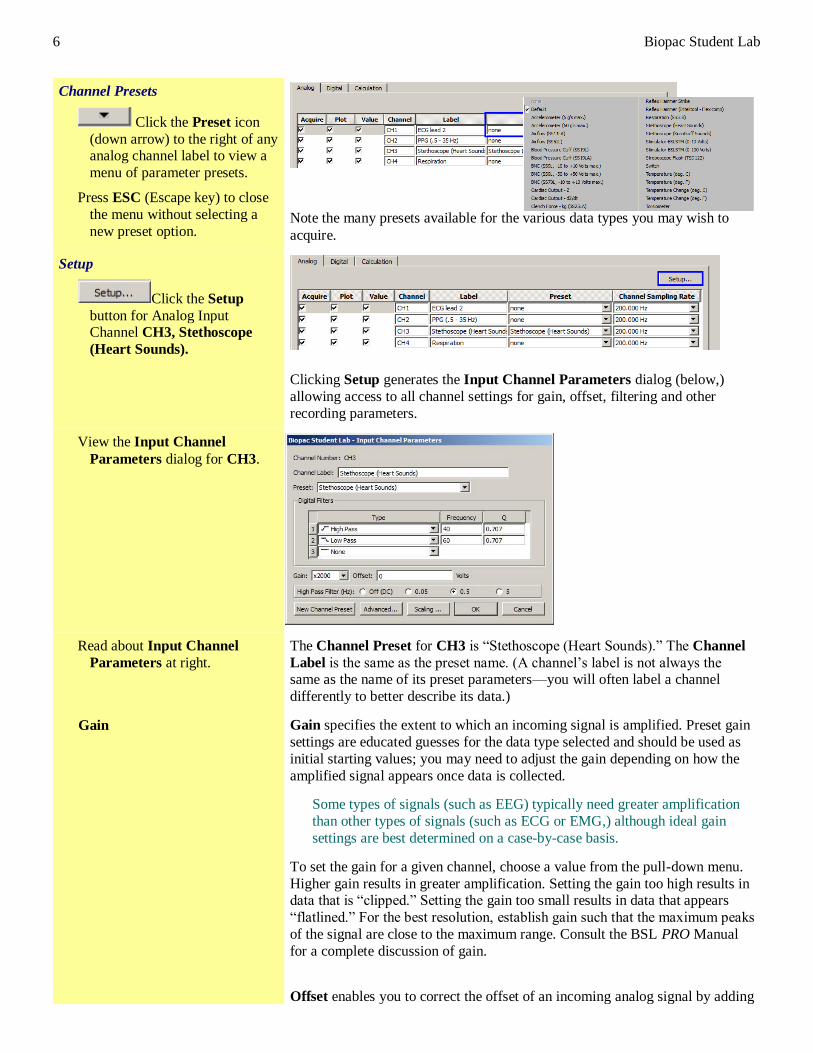
Channel Presets

Click the Preset icon

(down arrow) to the right of any analog channel label to view a

menu of parameter presets.

Press ESC (Escape key) to close

the menu without selecting a

new preset option.

Note the many presets available for the various data types you may wish to

acquire.

Setup

Click the Setup

button for Analog Input Channel CH3, Stethoscope

(Heart Sounds).

Clicking Setup generates the Input Channel Parameters dialog (below,)

allowing access to all channel settings for gain, offset, filtering and other

recording parameters.

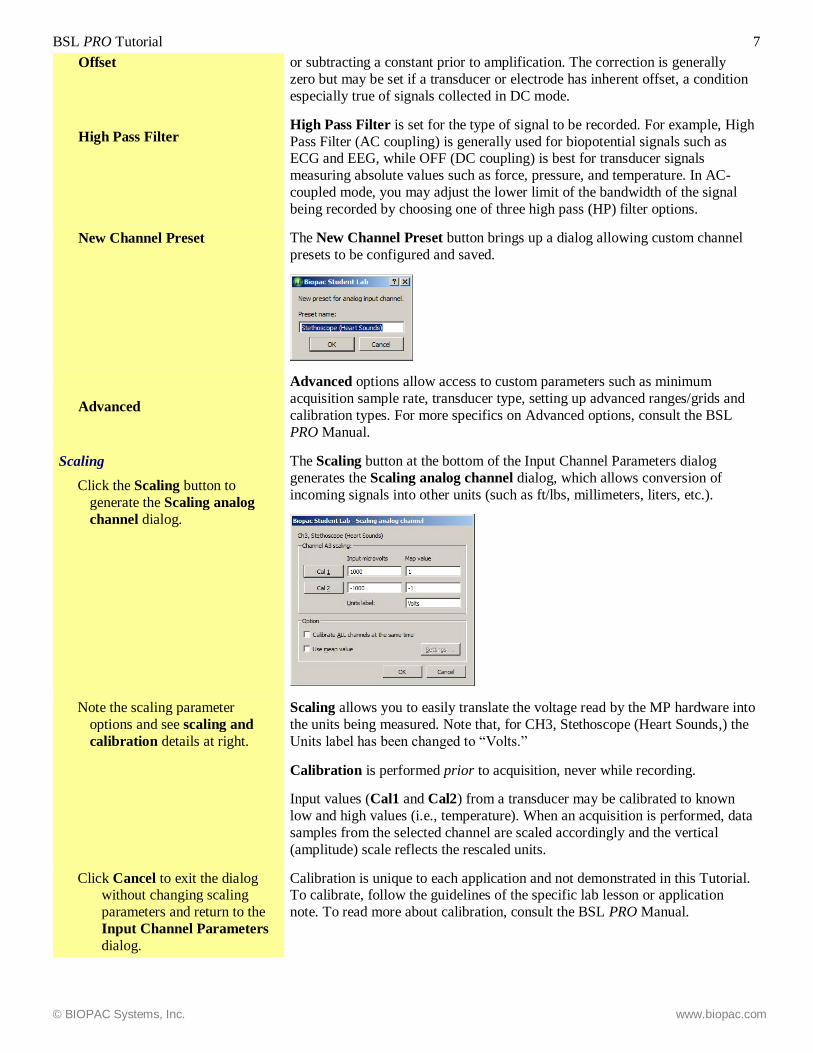
View the Input Channel

Parameters dialog for CH3.

Read about Input Channel

Parameters at right.

The Channel Preset for CH3 is “Stethoscope (Heart Sounds).” The Channel

Label is the same as the preset name. (A channel’s label is not always the same as the name of its preset parameters—you will often label a channel

differently to better describe its data.)

Gain

Gain specifies the extent to which an incoming signal is amplified. Preset gain

settings are educated guesses for the data type selected and should be used as

initial starting values; you may need to adjust the gain depending on how the

amplified signal appears once data is collected.

Some types of signals (such as EEG) typically need greater amplification

than other types of signals (such as ECG or EMG,) although ideal gain

settings are best determined on a case-by-case basis.

To set the gain for a given channel, choose a value from the pull-down menu.

Higher gain results in greater amplification. Setting the gain too high results in data that is “clipped.” Setting the gain too small results in data that appears

“flatlined.” For the best resolution, establish gain such that the maximum peaks

of the signal are close to the maximum range. Consult the BSL PRO Manual

for a complete discussion of gain.

Offset enables you to correct the offset of an incoming analog signal by adding

BSL PRO Tutorial 7


Offset

High Pass Filter

or subtracting a constant prior to amplification. The correction is generally

zero but may be set if a transducer or electrode has inherent offset, a condition

especially true of signals collected in DC mode.

High Pass Filter is set for the type of signal to be recorded. For example, High

Pass Filter (AC coupling) is generally used for biopotential signals such as ECG and EEG, while OFF (DC coupling) is best for transducer signals

measuring absolute values such as force, pressure, and temperature. In AC-

coupled mode, you may adjust the lower limit of the bandwidth of the signal

being recorded by choosing one of three high pass (HP) filter options.

New Channel Preset The New Channel Preset button brings up a dialog allowing custom channel

presets to be configured and saved.

Advanced

Advanced options allow access to custom parameters such as minimum

acquisition sample rate, transducer type, setting up advanced ranges/grids and

calibration types. For more specifics on Advanced options, consult the BSL

PRO Manual.

Scaling

Click the Scaling button to

generate the Scaling analog

channel dialog.

The Scaling button at the bottom of the Input Channel Parameters dialog

generates the Scaling analog channel dialog, which allows conversion of

incoming signals into other units (such as ft/lbs, millimeters, liters, etc.).

Note the scaling parameter

options and see scaling and

calibration details at right.

Scaling allows you to easily translate the voltage read by the MP hardware into

the units being measured. Note that, for CH3, Stethoscope (Heart Sounds,) the

Units label has been changed to “Volts.”

Calibration is performed prior to acquisition, never while recording.

Input values (Cal1 and Cal2) from a transducer may be calibrated to known

low and high values (i.e., temperature). When an acquisition is performed, data

samples from the selected channel are scaled accordingly and the vertical

(amplitude) scale reflects the rescaled units.

Click Cancel to exit the dialog without changing scaling

parameters and return to the

Input Channel Parameters

dialog.

Calibration is unique to each application and not demonstrated in this Tutorial. To calibrate, follow the guidelines of the specific lab lesson or application

note. To read more about calibration, consult the BSL PRO Manual.


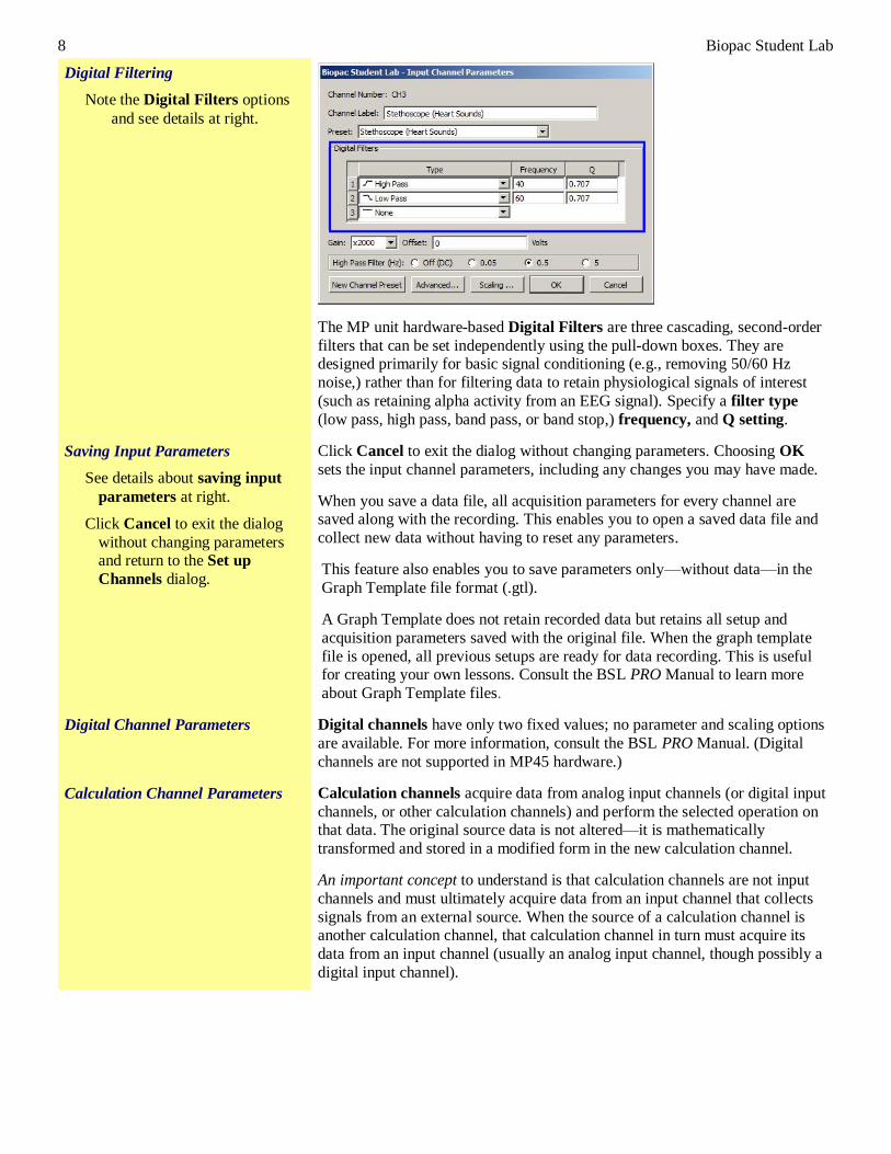
Digital Filtering

Note the Digital Filters options

and see details at right.

The MP unit hardware-based Digital Filters are three cascading, second-order

filters that can be set independently using the pull-down boxes. They are designed primarily for basic signal conditioning (e.g., removing 50/60 Hz

noise,) rather than for filtering data to retain physiological signals of interest

(such as retaining alpha activity from an EEG signal). Specify a filter type

(low pass, high pass, band pass, or band stop,) frequency, and Q setting.

Saving Input Parameters

See details about saving input

parameters at right.

Click Cancel to exit the dialog

without changing parameters and return to the Set up

Channels dialog.

Click Cancel to exit the dialog without changing parameters. Choosing OK

sets the input channel parameters, including any changes you may have made.

When you save a data file, all acquisition parameters for every channel are saved along with the recording. This enables you to open a saved data file and

collect new data without having to reset any parameters.

This feature also enables you to save parameters only—without data—in the

Graph Template file format (.gtl).

A Graph Template does not retain recorded data but retains all setup and

acquisition parameters saved with the original file. When the graph template

file is opened, all previous setups are ready for data recording. This is useful for creating your own lessons. Consult the BSL PRO Manual to learn more

about Graph Template files.

Digital Channel Parameters Digital channels have only two fixed values; no parameter and scaling options

are available. For more information, consult the BSL PRO Manual. (Digital

channels are not supported in MP45 hardware.)

Calculation Channel Parameters Calculation channels acquire data from analog input channels (or digital input

channels, or other calculation channels) and perform the selected operation on that data. The original source data is not altered—it is mathematically

transformed and stored in a modified form in the new calculation channel.

An important concept to understand is that calculation channels are not input

channels and must ultimately acquire data from an input channel that collects

signals from an external source. When the source of a calculation channel is another calculation channel, that calculation channel in turn must acquire its

data from an input channel (usually an analog input channel, though possibly a

digital input channel).

BSL PRO Tutorial 9


With the Calculation

Channel tab active, open the

Presets dialog (down arrow)

for Calculation Channel C1.

Choose the preset option ECG

R-R Interval.

For example, calculation channel C1 can be set up to compute the R-R Interval

of the ECG data on analog input channel CH1.

To do this, click the Preset icon (down arrow) to the right of Calculation

Channel C1 to generate a menu of calculation channel presets. Choose the

preset option “ECG R-R Interval.”

Click the Setup

button in the upper right corner

of the Calculation Channel

dialog to generate the Rate

dialog.

Choose the Signal Parameters

tab.

Note the Signal Parameters for

the ECG R-R Interval

calculation, and see details at

right.

Click Cancel to exit the dialog

without changing rate

parameters and return to the Set

up Channels dialog.

Note the Rate Signal Parameters dialog for the selected “ECG R-R

Interval” preset. The Source data for the calculation is acquired from “CH1,

ECG lead 2” and the Function (behind Output tab) is to compute the interval

in seconds.

Were you to record with these rate parameters, Analog Input Channel CH1

would acquire the ECG data from the subject, and Calculation Channel C1

would in turn compute the R-R Interval of the data collected on CH1.

Uncheck the Acquire, Plot and

Value boxes in the Calculation

Channel tab.

Click the close button to exit the

Input channels setup dialog

and return to the graph window.

Unchecking the “Acquire” option turns off the calculation channel. It will no

longer acquire, plot, nor display data.


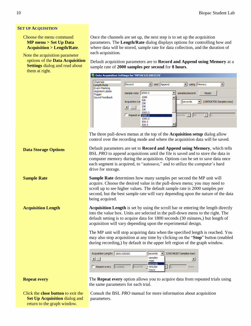
SET UP ACQUISITION


MP menu > Set Up Data

Acquisition > Length/Rate.

Note the acquisition parameter

options of the Data Acquisition

Settings dialog and read about

them at right.

Once the channels are set up, the next step is to set up the acquisition

parameters. The Length/Rate dialog displays options for controlling how and where data will be stored, sample rate for data collection, and the duration of

each acquisition.

Default acquisition parameters are to Record and Append using Memory at a

sample rate of 2000 samples per second for 8 hours.

Data Storage Options

The three pull-down menus at the top of the Acquisition setup dialog allow

control over the recording mode and where the acquisition data will be saved.

Default parameters are set to Record and Append using Memory, which tells

BSL PRO to append acquisitions until the file is saved and to store the data in

computer memory during the acquisition. Options can be set to save data once

each segment is acquired, to “autosave,” and to utilize the computer’s hard

drive for storage.

Sample Rate Sample Rate determines how many samples per second the MP unit will

acquire. Choose the desired value in the pull-down menu; you may need to

scroll up to see higher values. The default sample rate is 2000 samples per

second, but the best sample rate will vary depending upon the nature of the data

being acquired.

Acquisition Length Acquisition Length is set by using the scroll bar or entering the length directly

into the value box. Units are selected in the pull-down menu to the right. The

default setting is to acquire data for 1800 seconds (30 minutes,) but length of

acquisition will vary depending upon the experimental design.

The MP unit will stop acquiring data when the specified length is reached. You may also stop acquisition at any time by clicking on the “Stop” button (enabled

during recording,) by default in the upper left region of the graph window.

Repeat every The Repeat every option allows you to acquire data from repeated trials using

the same parameters for each trial.

Click the close button to exit the Set Up Acquisition dialog and

return to the graph window.

Consult the BSL PRO manual for more information about acquisition

parameters.

BSL PRO Tutorial 11


TRIGGERING, OUTPUT CONTROL,

AND OTHER MP MENU OPTIONS

Click on the MP menu and view

other available commands. Read

about them at right.

Note the options on the MP menu and read about some of them below.

• MP45 Users: MP45 menu commands differ from those available for the

MP36/35. Consult the BSL PRO Manual for more information.

Set up Triggering allows you to start an acquisition “on cue” from a trigger

device connected to the MP unit. (Not supported in MP45 hardware.)

Access Triggering via MP menu > Set Up Data Acquisition > Trigger.

Show Input Values opens a window that displays input data in numerical

format as it is being acquired. (This function is enabled only when the “Show

Input Values” option for a channel is enabled in the Input channel parameters

dialog.)

Output Control generates a submenu of Output Controls. The MP36/35

outputs signals via ports on its back panel. To output analog signals, use the

“Analog Out” port; to output digital signals, use the “I/O” port.

• Available output controls for the MP36/35 are CH to Output, Voltage,

Digital Outputs, Pulses, Stimulator-BSLSTM, Pulse Sequence, Human Stimulator – STMHUM, Visual Stim Controllable LED –

OUT4, Arbitrary Wave Output, Sound Sequence and Low Voltage

Stimulator. Consult the BSL PRO Manual for more information. (Pulse

Sequence is available only on MP36/MP35A hardware. Voltage is

available in MP35 only.)

Part 2: Recording

See details about recording data at

right.

If the MP unit is not connected,

review recording details at right

and proceed to the following

section.

Once the input channels and acquisition parameters are set up, you are ready to

record. To acquire data, the MP unit must be connected to your computer and powered on. (If the MP unit is not properly connected or not communicating

with your computer, you will be unable to record data and an error prompt will

appear.)

Recording a file is beyond the scope of this tutorial, other than to practice

acquiring a few segments of “flatline” practice data.

• To acquire useful data, electrodes, transducers and other devices must be

in place to collect signals from your subject. If no input devices (e.g. electrodes or transducers) are connected to the MP unit, but the MP unit is

connected to the computer, the unit will acquire—and BSL PRO will

display—a small, “flatline” value of random signal “noise” with a mean of

about 0.0 Volts.

If the MP data acquisition unit is

connected, practice recording a

new data file.

• Choose File > New to open an

“Untitled” graph window and

practice recording.

• Use the Start/Stop button in

the graph window to acquire

multiple, short segments of

“flatline” practice data.

• Use the Rewind button in the

Toolbar to delete a data

segment.

If the MP unit is connected, choose File > New to open an “Untitled” graph

window and practice recording data. If no MP unit is connected, read about

recording below and proceed to the following section of this tutorial.

Start acquisition by clicking the Start button in the upper left

corner of the graph window, or by pressing “Ctrl + Spacebar.” The circle next to the Start/Stop button, when green and solid, indicates that the MP hardware

is communicating with the computer, ready to record.

Once an acquisition has started the Start/Stop button in the graph window

changes to Stop. (The two opposing arrows to the left of the button indicate

that data is being collected. The “Busy” status light on the front of the MP unit

also indicates that data is being collected.)


• Choose File > Close to close

the practice graph without

saving.

Stop an acquisition at any time by clicking the Stop button, or by

pressing “Ctrl + Spacebar.” An acquisition automatically stops when it

reaches the Acquisition Length parameter in the Set up Acquisition dialog.

In the default Append mode, BSL PRO can record multiple segments in a

single file. Simply “Start” again to append another recording segment. An

append marker indicates the beginning of each new recording segment.

The Rewind button to the right of the Start button deletes the last

recorded segment.

Acquisition parameters cannot be changed while recording is in progress. If

acquisition parameters are modified during a pause between recording segments, and then the recording is restarted, BSL will warn that previous data

will be overwritten (unless the “Warn on Overwrite” option in the MP menu is

disabled). Similarly, deleting a recorded segment with the Rewind command

will generate a warning.

After recording multiple short segments, choose File > Close to close the

practice data window without saving.

Recording is unique to each application. Follow the recording guidelines for

your specific lab lesson, experiment, or application note. To read more about

recording, consult the BSL PRO Manual.

Part 3: Display The BSL PRO graph window is designed to provide you with a powerful yet

easy-to-use interface for viewing and manipulating data.

Note the features of the BSL PRO

display in the labeled figure at

right.

BSL PRO Tutorial 13


CHANNELS

Selecting Channels

Note the four channels of data in

the display of sample file

4Channel.acq.

Click the CH2 channel number

box (or its “PPG” label to the

left of the waveform) to make it

the active channel.

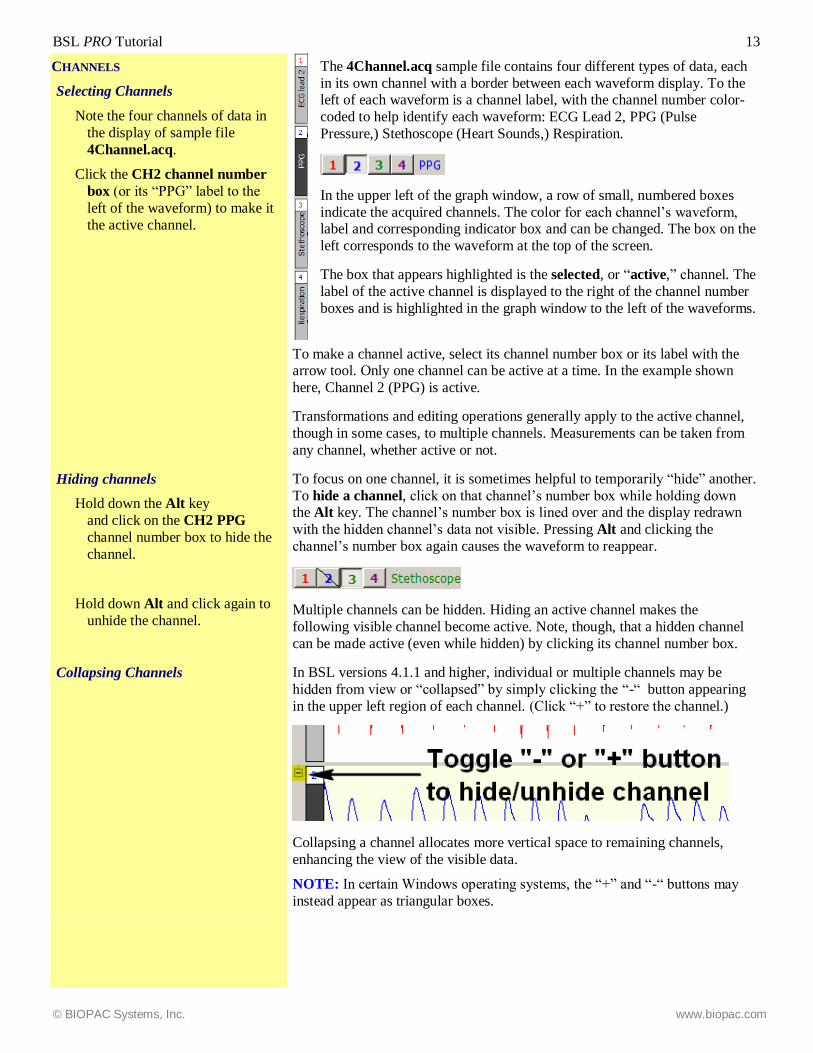
The 4Channel.acq sample file contains four different types of data, each

in its own channel with a border between each waveform display. To the left of each waveform is a channel label, with the channel number color-

coded to help identify each waveform: ECG Lead 2, PPG (Pulse

Pressure,) Stethoscope (Heart Sounds,) Respiration.

In the upper left of the graph window, a row of small, numbered boxes

indicate the acquired channels. The color for each channel’s waveform, label and corresponding indicator box and can be changed. The box on the

left corresponds to the waveform at the top of the screen.

The box that appears highlighted is the selected, or “active,” channel. The

label of the active channel is displayed to the right of the channel number

boxes and is highlighted in the graph window to the left of the waveforms.

To make a channel active, select its channel number box or its label with the arrow tool. Only one channel can be active at a time. In the example shown

here, Channel 2 (PPG) is active.

Transformations and editing operations generally apply to the active channel,

though in some cases, to multiple channels. Measurements can be taken from

any channel, whether active or not.

Hiding channels

Hold down the Alt key

and click on the CH2 PPG

channel number box to hide the

channel.

Hold down Alt and click again to

unhide the channel.

To focus on one channel, it is sometimes helpful to temporarily “hide” another.

To hide a channel, click on that channel’s number box while holding down the Alt key. The channel’s number box is lined over and the display redrawn

with the hidden channel’s data not visible. Pressing Alt and clicking the

channel’s number box again causes the waveform to reappear.

Multiple channels can be hidden. Hiding an active channel makes the

following visible channel become active. Note, though, that a hidden channel

can be made active (even while hidden) by clicking its channel number box.

Collapsing Channels In BSL versions 4.1.1 and higher, individual or multiple channels may be

hidden from view or “collapsed” by simply clicking the “-“ button appearing

in the upper left region of each channel. (Click “+” to restore the channel.)

Collapsing a channel allocates more vertical space to remaining channels,

enhancing the view of the visible data.

NOTE: In certain Windows operating systems, the “+” and “-“ buttons may

instead appear as triangular boxes.


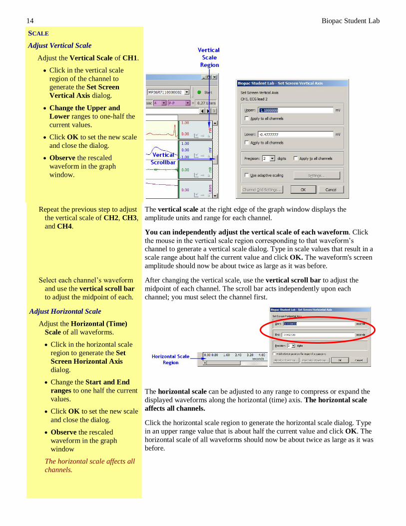
SCALE

Adjust Vertical Scale

Adjust the Vertical Scale of CH1.

• Click in the vertical scale

region of the channel to generate the Set Screen

Vertical Axis dialog.

• Change the Upper and

Lower ranges to one-half the

current values.

• Click OK to set the new scale

and close the dialog.

• Observe the rescaled

waveform in the graph

window.

Repeat the previous step to adjust

the vertical scale of CH2, CH3,

and CH4.

The vertical scale at the right edge of the graph window displays the

amplitude units and range for each channel.

You can independently adjust the vertical scale of each waveform. Click

the mouse in the vertical scale region corresponding to that waveform’s channel to generate a vertical scale dialog. Type in scale values that result in a

scale range about half the current value and click OK. The waveform's screen

amplitude should now be about twice as large as it was before.

Select each channel’s waveform

and use the vertical scroll bar

to adjust the midpoint of each.

After changing the vertical scale, use the vertical scroll bar to adjust the

midpoint of each channel. The scroll bar acts independently upon each

channel; you must select the channel first.

Adjust Horizontal Scale

Adjust the Horizontal (Time)

Scale of all waveforms.

• Click in the horizontal scale

region to generate the Set

Screen Horizontal Axis

dialog.

• Change the Start and End

ranges to one half the current

values.

• Click OK to set the new scale

and close the dialog.

• Observe the rescaled

waveform in the graph

window

The horizontal scale affects all

channels.

The horizontal scale can be adjusted to any range to compress or expand the

displayed waveforms along the horizontal (time) axis. The horizontal scale

affects all channels.

Click the horizontal scale region to generate the horizontal scale dialog. Type

in an upper range value that is about half the current value and click OK. The

horizontal scale of all waveforms should now be about twice as large as it was

before.

BSL PRO Tutorial 15


Use the horizontal scroll bar

to scroll to the beginning and

end of the recording.

Adjusting horizontal scale allows you to magnify the screen display to better

examine a waveform but note that the waveforms may no longer fit in the data

window. The file, however, contains the complete record even if all data is not

displayed on the screen.

To view the beginning of the recording (time zero,) scroll left with the horizontal scroll bar. To view the end, scroll right. The horizontal (time)

scale along the bottom of the graph window denotes when the data was

recorded relative to the beginning of the acquisition.

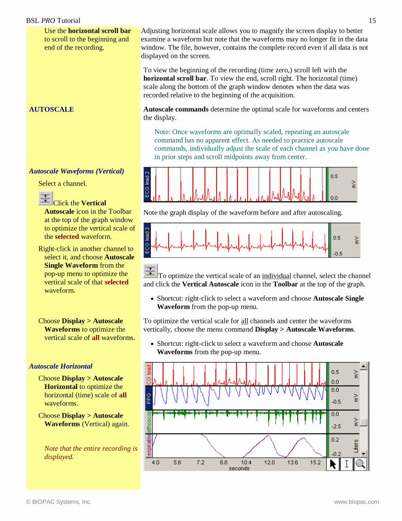
AUTOSCALE Autoscale commands determine the optimal scale for waveforms and centers

the display.

Note: Once waveforms are optimally scaled, repeating an autoscale

command has no apparent effect. As needed to practice autoscale commands, individually adjust the scale of each channel as you have done

in prior steps and scroll midpoints away from center.

Autoscale Waveforms (Vertical)

Select a channel.

Click the Vertical

Autoscale icon in the Toolbar

at the top of the graph window

to optimize the vertical scale of

the selected waveform.

Right-click in another channel to

select it, and choose Autoscale

Single Waveform from the

pop-up menu to optimize the

vertical scale of that selected

waveform.

Note the graph display of the waveform before and after autoscaling.

To optimize the vertical scale of an individual channel, select the channel

and click the Vertical Autoscale icon in the Toolbar at the top of the graph.

• Shortcut: right-click to select a waveform and choose Autoscale Single

Waveform from the pop-up menu.

Choose Display > Autoscale

Waveforms to optimize the

vertical scale of all waveforms.

To optimize the vertical scale for all channels and center the waveforms

vertically, choose the menu command Display > Autoscale Waveforms.

• Shortcut: right-click to select a waveform and choose Autoscale

Waveforms from the pop-up menu.

Autoscale Horizontal


Horizontal to optimize the

horizontal (time) scale of all

waveforms.


Waveforms (Vertical) again.

Note that the entire recording is

displayed.


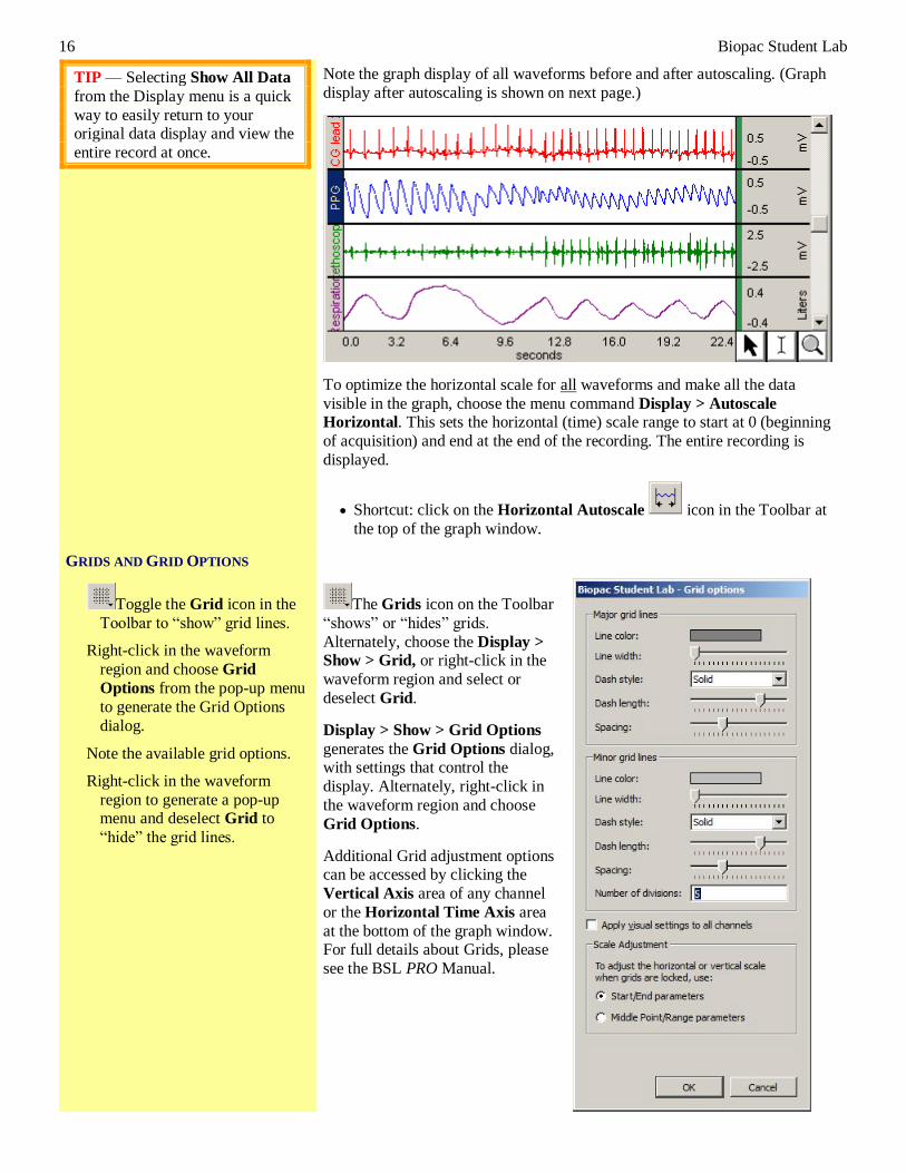
TIP — Selecting Show All Data

from the Display menu is a quick

way to easily return to your original data display and view the

entire record at once.

Note the graph display of all waveforms before and after autoscaling. (Graph

display after autoscaling is shown on next page.)

To optimize the horizontal scale for all waveforms and make all the data

visible in the graph, choose the menu command Display > Autoscale

Horizontal. This sets the horizontal (time) scale range to start at 0 (beginning

of acquisition) and end at the end of the recording. The entire recording is

displayed.

• Shortcut: click on the Horizontal Autoscale icon in the Toolbar at

the top of the graph window.

GRIDS AND GRID OPTIONS

Toggle the Grid icon in the

Toolbar to “show” grid lines.

Right-click in the waveform

region and choose Grid

Options from the pop-up menu

to generate the Grid Options

dialog.

Note the available grid options.

Right-click in the waveform

region to generate a pop-up menu and deselect Grid to

“hide” the grid lines.

The Grids icon on the Toolbar

“shows” or “hides” grids.

Alternately, choose the Display >

Show > Grid, or right-click in the

waveform region and select or

deselect Grid.

Display > Show > Grid Options

generates the Grid Options dialog, with settings that control the

display. Alternately, right-click in

the waveform region and choose

Grid Options.

Additional Grid adjustment options can be accessed by clicking the

Vertical Axis area of any channel

or the Horizontal Time Axis area

at the bottom of the graph window. For full details about Grids, please

see the BSL PRO Manual.

BSL PRO Tutorial 17


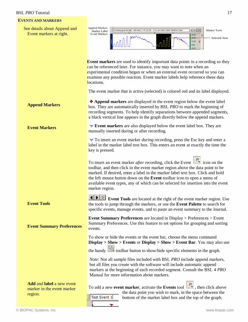
EVENTS AND MARKERS

See details about Append and

Event markers at right.

Append Markers

Event Markers

Event Tools

Event Summary Preferences

Event markers are used to identify important data points in a recording so they

can be referenced later. For instance, you may want to note when an

experimental condition began or when an external event occurred so you can

examine any possible reaction. Event marker labels help reference these data

locations.

The event marker that is active (selected) is colored red and its label displayed.

Append markers are displayed in the event region below the event label

box. They are automatically inserted by BSL PRO to mark the beginning of

recording segments. To help identify separations between appended segments,

a black vertical line appears in the graph directly below the append markers.

Event markers are also displayed below the event label box. They are

manually inserted during or after recording.

To insert an event marker during recording, press the Esc key and enter a

label in the marker label text box. This enters an event at exactly the time the

key is pressed.

To insert an event marker after recording, click the Event icon on the

toolbar, and then click in the event marker region above the data point to be marked. If desired, enter a label in the marker label text box. Click and hold

the left mouse button down on the Event toolbar icon to open a menu of

available event types, any of which can be selected for insertion into the event

marker region.

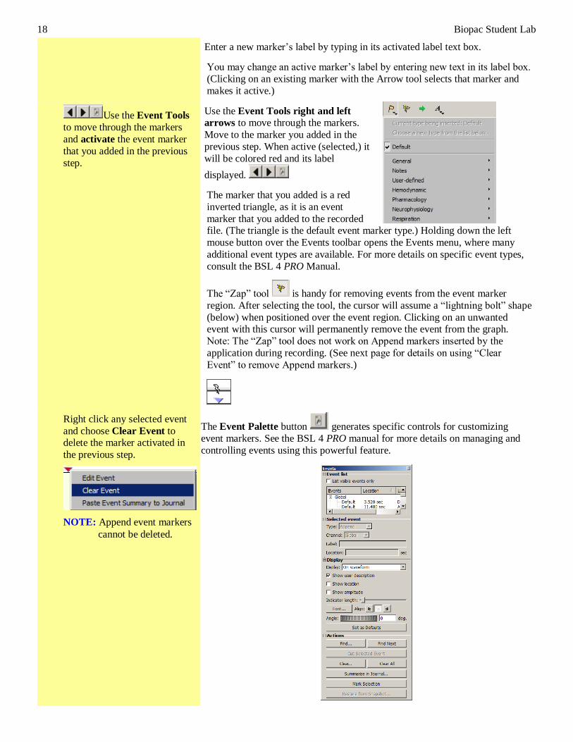
Event Tools are located at the right of the event marker region. Use

the tools to jump through the markers, or use the Event Palette to search for

specific events, manage events, and to paste an event summary to the Journal.

Event Summary Preferences are located in Display > Preferences > Event

Summary Preferences. Use this feature to set options for grouping and sorting

events.

To show or hide the events or the event bar, choose the menu command

Display > Show > Events or Display > Show > Event Bar. You may also use

the handy toolbar button to show/hide specific elements in the graph.

Note: Not all sample files included with BSL PRO include append markers,

but all files you create with the software will include automatic append

markers at the beginning of each recorded segment. Consult the BSL 4 PRO

Manual for more information about markers.

Add and label a new event marker in the event marker

region.

To add a new event marker, activate the Events tool , then click above the data point you wish to mark, in the space between the

bottom of the marker label box and the top of the graph.


Enter a new marker’s label by typing in its activated label text box.

You may change an active marker’s label by entering new text in its label box.

(Clicking on an existing marker with the Arrow tool selects that marker and

makes it active.)

Use the Event Tools

to move through the markers

and activate the event marker

that you added in the previous

step.

Use the Event Tools right and left

arrows to move through the markers.

Move to the marker you added in the

previous step. When active (selected,) it

will be colored red and its label

displayed.

The marker that you added is a red

inverted triangle, as it is an event

marker that you added to the recorded file. (The triangle is the default event marker type.) Holding down the left

mouse button over the Events toolbar opens the Events menu, where many

additional event types are available. For more details on specific event types,

consult the BSL 4 PRO Manual.

The “Zap” tool is handy for removing events from the event marker

region. After selecting the tool, the cursor will assume a “lightning bolt” shape

(below) when positioned over the event region. Clicking on an unwanted event with this cursor will permanently remove the event from the graph.

Note: The “Zap” tool does not work on Append markers inserted by the

application during recording. (See next page for details on using “Clear

Event” to remove Append markers.)

Right click any selected event

and choose Clear Event to delete the marker activated in

the previous step.

NOTE: Append event markers

cannot be deleted.

The Event Palette button generates specific controls for customizing

event markers. See the BSL 4 PRO manual for more details on managing and

controlling events using this powerful feature.

BSL PRO Tutorial 19


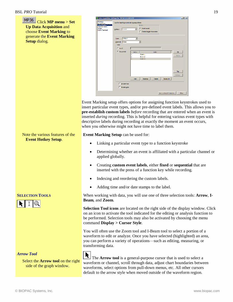
Click MP menu > Set

Up Data Acquisition and

choose Event Marking to generate the Event Marking

Setup dialog.

Event Marking setup offers options for assigning function keystrokes used to

insert particular event types, and/or pre-defined event labels. This allows you to

pre-establish custom labels before recording that are entered when an event is inserted during recording. This is helpful for entering various event types with

descriptive labels during recording at exactly the moment an event occurs,

when you otherwise might not have time to label them.

Note the various features of the

Event Hotkey Setup. Event Marking Setup can be used for:

• Linking a particular event type to a function keystroke

• Determining whether an event is affiliated with a particular channel or

applied globally.

• Creating custom event labels, either fixed or sequential that are

inserted with the press of a function key while recording.

• Indexing and reordering the custom labels.

• Adding time and/or date stamps to the label.

SELECTION TOOLS

When working with data, you will use one of three selection tools: Arrow, I-

Beam, and Zoom.

Selection Tool icons are located on the right side of the display window. Click

on an icon to activate the tool indicated for the editing or analysis function to be performed. Selection tools may also be activated by choosing the menu

command Display > Cursor Style.

You will often use the Zoom tool and I-Beam tool to select a portion of a

waveform to edit or analyze. Once you have selected (highlighted) an area,

you can perform a variety of operations—such as editing, measuring, or

transforming data.

Arrow Tool

Select the Arrow tool on the right

side of the graph window.

The Arrow tool is a general-purpose cursor that is used to select a

waveform or channel, scroll through data, adjust chart boundaries between

waveforms, select options from pull-down menus, etc. All other cursors

default to the arrow style when moved outside of the waveform region.


Use the Arrow tool to resize the

chart boundaries between

waveforms.

Choose Display > Reset Chart

Display to return the display to

equal sized waveform “tracks.”

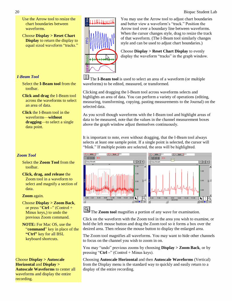
You may use the Arrow tool to adjust chart boundaries

and better view a waveform’s “track.” Position the Arrow tool over a boundary line between waveforms.

When the cursor changes style, drag to resize the track

of that waveform. (The I-Beam tool similarly changes

style and can be used to adjust chart boundaries.)

Choose Display > Reset Chart Display to evenly

display the waveform “tracks” in the graph window.

I-Beam Tool

Select the I-Beam tool from the

toolbar.

Click and drag the I-Beam tool across the waveforms to select

an area of data.

Click the I-Beam tool in the

waveforms—without

dragging—to select a single

data point.

The I-Beam tool is used to select an area of a waveform (or multiple

waveforms) to be edited, measured, or transformed.

Clicking and dragging the I-Beam tool across waveforms selects and

highlights an area of data. You can perform a variety of operations (editing,

measuring, transforming, copying, pasting measurements to the Journal) on the

selected data.

As you scroll though waveforms with the I-Beam tool and highlight areas of

data to be measured, note that the values in the channel measurement boxes

above the graph window adjust themselves continuously.

It is important to note, even without dragging, that the I-Beam tool always selects at least one sample point. If a single point is selected, the cursor will

“blink.” If multiple points are selected, the area will be highlighted.

Zoom Tool

Select the Zoom Tool from the

toolbar.

Click, drag, and release the

Zoom tool in a waveform to

select and magnify a section of

data.

Zoom again.

Choose Display > Zoom Back,

or press “Ctrl –” (Control + Minus keys,) to undo the

previous Zoom command.

NOTE: For Mac OS, use the “command” key in place of the

“Ctrl” key for all BSL

keyboard shortcuts.

The Zoom tool magnifies a portion of any wave for examination.

Click on the waveform with the Zoom tool in the area you wish to examine, or

hold the left mouse button and drag the Zoom tool so it forms a box over the

desired area. Then release the mouse button to display the enlarged area.

The Zoom tool magnifies all waveforms. You may want to hide other channels

to focus on the channel you wish to zoom in on.

You may “undo” previous zooms by choosing Display > Zoom Back, or by

pressing “Ctrl –” (Control + Minus keys).


Horizontal and Display >

Autoscale Waveforms to center all waveforms and display the entire

recording.

Choosing Autoscale Horizontal and then Autoscale Waveforms (Vertical)

from the Display menu is the standard way to quickly and easily return to a

display of the entire recording.

BSL PRO Tutorial 21


MEASUREMENTS

Over 30 measurement types are available in BSL PRO via the Measurements

pull-down menu. Some measurements (such as Time or Value) look at only a single data point whereas other measurements (such as Mean and Delta T)

examine a selected range of data.

Measurement features can be automated so that measurements are taken and pasted into the Journal file when a specific event occurs, or at pre-specified,

user-defined time intervals.

Measurement Boxes

Read about measurement boxes

at the right.

The measurement region is located near the top of the graph window. For

each measurement, there are pull-down boxes that specify the channel to be

measured and type of measurement, and a value box that displays the results.

To specify the channel to be measured, click on the channel selection box and choose from the pull-down menu. When the designation “SC” is chosen

(default,) measurements are taken from the channel that is active, or

“selected,” in the graph window.

To specify a measurement type, click on the measurement box and choose

from the pull-down menu.

Measurement results are displayed in the box to the right of the

measurement type. Results reflect the waveform data selected in the graph

window with the I-Beam tool.

Taking Measurements

Note the measurement boxes in

the 4channel.acq sample file.

As you drag the I-Beam tool across waveforms, note the

change in values in the channel

measurement boxes.

The sample file 4Channel.acq displays five measurement boxes in the region

below the Toolbar. The first is configured to measure CH1 Delta, the second to measure CH1 BPM, the third CH3 P-P, the fourth CH4 Delta T, and the

fifth CH4 P-P.

• If all five measurement boxes are not displayed, drag the window wider.

The measurements adjust themselves continuously as you scroll through the

waveforms with the I-Beam tool, reflecting the area of data highlighted in the

graph window.

It is important to note that the I-Beam always selects either a single point or

an area spanning multiple sample points. When a single point is selected, the cursor will “blink.” When multiple points are selected, the area will be

highlighted. If an area is defined and a single point measurement is selected,

such as X-axis T (Time,) the measurement will reflect the last selected point.


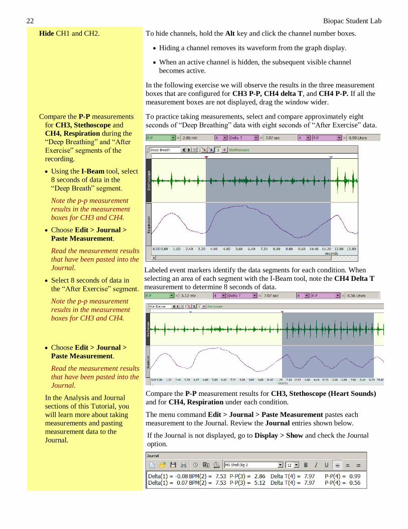
Hide CH1 and CH2. To hide channels, hold the Alt key and click the channel number boxes.

• Hiding a channel removes its waveform from the graph display.

• When an active channel is hidden, the subsequent visible channel

becomes active.

In the following exercise we will observe the results in the three measurement

boxes that are configured for CH3 P-P, CH4 delta T, and CH4 P-P. If all the

measurement boxes are not displayed, drag the window wider.

Compare the P-P measurements

for CH3, Stethoscope and CH4, Respiration during the

“Deep Breathing” and “After

Exercise” segments of the

recording.

• Using the I-Beam tool, select

8 seconds of data in the

“Deep Breath” segment.

Note the p-p measurement

results in the measurement

boxes for CH3 and CH4.

• Choose Edit > Journal >

Paste Measurement.

Read the measurement results

that have been pasted into the

Journal.

• Select 8 seconds of data in

the “After Exercise” segment.

Note the p-p measurement

results in the measurement

boxes for CH3 and CH4.

• Choose Edit > Journal >

Paste Measurement.

Read the measurement results

that have been pasted into the

Journal.

In the Analysis and Journal

sections of this Tutorial, you

will learn more about taking measurements and pasting

measurement data to the

Journal.

To practice taking measurements, select and compare approximately eight

seconds of “Deep Breathing” data with eight seconds of “After Exercise” data.

Labeled event markers identify the data segments for each condition. When

selecting an area of each segment with the I-Beam tool, note the CH4 Delta T measurement to determine 8 seconds of data.

Compare the P-P measurement results for CH3, Stethoscope (Heart Sounds)

and for CH4, Respiration under each condition.

The menu command Edit > Journal > Paste Measurement pastes each

measurement to the Journal. Review the Journal entries shown below.

If the Journal is not displayed, go to Display > Show and check the Journal

option.

BSL PRO Tutorial 23


Part 4: Analysis

ANALYSIS OVERVIEW One advantage of saving data files to disk is that you can quickly and easily

perform post-hoc analyses of your recorded data. BSL PRO software is a

powerful and flexible analytical tool designed to provide you with immediate

feedback from each operation. Using BSL PRO, you are able to...

• Use digital filtering and smoothing.

• Find patterns within data sets.

• Automatically find peaks and calculate rate data.

• Perform mathematical and statistical operations.

• Log results and observations to a journal.

• Mark events during acquisition or analysis.

• Transform data after it has been acquired.

To get an idea of how BSL PRO provides immediate feedback, run a Find

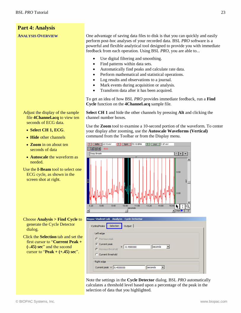
Cycle function on the 4Channel.acq sample file.

Adjust the display of the sample

file 4Channel.acq to view ten

seconds of ECG data.

• Select CH 1, ECG.

• Hide other channels

• Zoom in on about ten

seconds of data

• Autoscale the waveform as

needed.

Use the I-Beam tool to select one

ECG cycle, as shown in the

screen shot at right.

Select CH 1 and hide the other channels by pressing Alt and clicking the

channel number boxes.

Use the Zoom tool to examine a 10-second portion of the waveform. To center your display after zooming, use the Autoscale Waveforms (Vertical)

command from the Toolbar or from the Display menu.

Choose Analysis > Find Cycle to

generate the Cycle Detector

dialog.

Click the Selection tab and set the

first cursor to “Current Peak +

(-.45) sec” and the second

cursor to “Peak + (+.45) sec”.

Note the settings in the Cycle Detector dialog. BSL PRO automatically

calculates a threshold level based upon a percentage of the peak in the

selection of data that you highlighted.


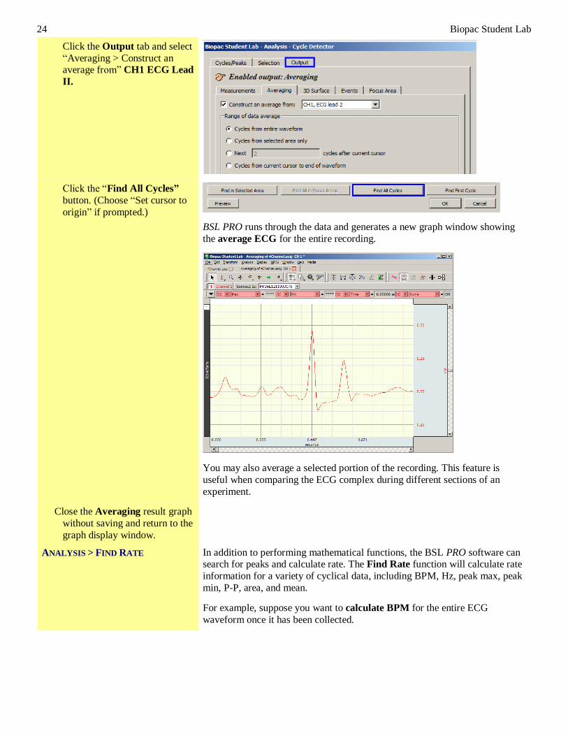
Click the Output tab and select

“Averaging > Construct an average from” CH1 ECG Lead

II.

Click the “Find All Cycles”

button. (Choose “Set cursor to

origin” if prompted.)

BSL PRO runs through the data and generates a new graph window showing

the average ECG for the entire recording.

You may also average a selected portion of the recording. This feature is

useful when comparing the ECG complex during different sections of an

experiment.

Close the Averaging result graph

without saving and return to the

graph display window.

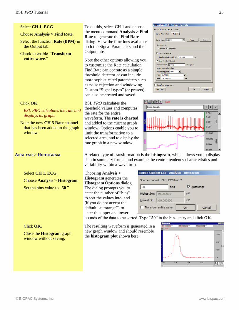
ANALYSIS > FIND RATE In addition to performing mathematical functions, the BSL PRO software can search for peaks and calculate rate. The Find Rate function will calculate rate

information for a variety of cyclical data, including BPM, Hz, peak max, peak

min, P-P, area, and mean.

For example, suppose you want to calculate BPM for the entire ECG

waveform once it has been collected.

BSL PRO Tutorial 25


Select CH 1, ECG.

Choose Analysis > Find Rate.

Select the function Rate (BPM) in

the Output tab.

Check to enable “Transform

entire wave.”

To do this, select CH 1 and choose

the menu command Analysis > Find

Rate to generate the Find Rate

dialog. View the functions available both the Signal Parameters and the

Output tabs.

Note the other options allowing you

to customize the Rate calculation.

Find Rate can operate as a simple threshold detector or can include

more sophisticated parameters such

as noise rejection and windowing.

Custom “Signal types” (or presets)

can also be created and saved.

Click OK.

BSL PRO calculates the rate and

displays its graph.

Note the new CH 5 Rate channel

that has been added to the graph

window.

BSL PRO calculates the

threshold values and computes

the rate for the entire

waveform. The rate is charted and added to the current graph

window. Options enable you to

limit the transformation to a selected area, and to display the

rate graph in a new window.

ANALYSIS > HISTOGRAM A related type of transformation is the histogram, which allows you to display

data in summary format and examine the central tendency characteristics and

variability within a waveform.

Select CH 1, ECG.

Choose Analysis > Histogram.

Set the bins value to “50.”

Choosing Analysis >

Histogram generates the Histogram Options dialog.

The dialog prompts you to

enter the number of “bins”

to sort the values into, and (if you do not accept the

default “autorange”) to

enter the upper and lower

bounds of the data to be sorted. Type “50” in the bins entry and click OK.

Click OK.

Close the Histogram graph

window without saving.

The resulting waveform is generated in a

new graph window and should resemble

the histogram plot shown here.


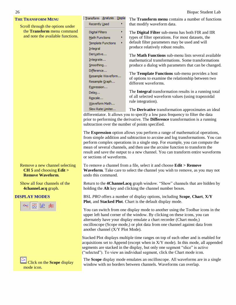
THE TRANSFORM MENU

Scroll through the options under

the Transform menu command

and note the available functions.

The Transform menu contains a number of functions

that modify waveform data.

The Digital Filter sub-menu has both FIR and IIR

types of filter operations. For most datasets, the default filter parameters may be used and will

produce relatively robust results.

The Math Functions sub-menu lists several available

mathematical transformations. Some transformations

produce a dialog with parameters that can be changed.

The Template Functions sub-menu provides a host of options to examine the relationship between two

different waveforms.

The Integral transformation results in a running total

of all selected waveform values (using trapezoidal

rule integration).

The Derivative transformation approximates an ideal

differentiator. It allows you to specify a low pass frequency to filter the data prior to performing the derivative. The Difference transformation is a running

subtraction over the number of points specified.

The Expression option allows you perform a range of mathematical operations,

from simple addition and subtraction to arcsine and log transformations. You can

perform complex operations in a single step. For example, you can compute the mean of several channels, and then use the arcsine function to transform the

result and save the output to a new channel. You can transform entire waveforms

or sections of waveforms.

Remove a new channel selecting

CH 5 and choosing Edit >

Remove Waveform.

To remove a channel from a file, select it and choose Edit > Remove

Waveform. Take care to select the channel you wish to remove, as you may not

undo this command.

Show all four channels of the

4channel.acq graph.

Return to the 4Channel.acq graph window. “Show” channels that are hidden by

holding the Alt key and clicking the channel number boxes.

DISPLAY MODES

BSL PRO offers a number of display options, including Scope, Chart, X/Y

Plot, and Stacked Plot. Chart is the default display mode.

You can switch from one display mode to another using the Toolbar icons in the

upper left hand corner of the window. By clicking on these icons, you can

alternately have your display emulate a chart recorder (Chart mode,)

oscilloscope (Scope mode,) or plot data from one channel against data from

another channel (X/Y Plot Mode).

Stacked Plot displays multiple time ranges on top of each other and is enabled for

acquisitions set to Append (except when in X/Y mode). In this mode, all appended

segments are stacked in the display, but only one segment “slice” is active

(“selected”). To view an individual segment, click the Chart mode icon.

Click on the Scope display

mode icon.

The Scope display mode emulates an oscilloscope. All waveforms are in a single

window with no borders between channels. Waveforms can overlap.

BSL PRO Tutorial 27


• Choose Display > Tile

Waveforms

• Choose Display > Overlap

Waveforms

• Hide CH 1 and CH 2.

• Analyze the CH 3 and CH 4

waveforms.

Display menu options determine the display of waveform data.

Analyze the relationship between CH 3, Stethoscope (Heart Sounds) and CH

4, Respiration. Note the differences between the “Deep Breath” and “After

Exercise” data segments.

Click on the X/Y Plot display

mode icon.

• Set the X-axis to

“Respiration.”

• Set the Y-axis to

“Stethoscope.”

X/Y Plots are useful for respiration studies, vectorcardiograms, and

investigations into non-linear dynamics.

In X/Y display mode, the X-axis and Y-axis labels correspond with the channels

that are being plotted. To set the axes, click on the labels and choose the channel

to plot from the pull-down menu.

In X/Y display mode, the I-Beam tool becomes a cross hair. When scrolled

across the graph window, the X-axis and Y-axis values are displayed in the

measurement region above the graph window.

Return to the Chart display

mode, show all channels, and

autoscale waveforms.

Click on the Chart display icon to return to Chart mode. Show any hidden

channels by holding the Alt key and clicking the channel number boxes.

Choose Display > Show All Data to optimally scale and center all waveforms.

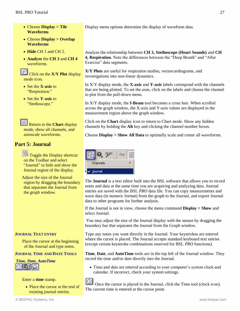
Part 5: Journal

Toggle the Display shortcut

on the Toolbar and select “Journal” to hide and show the

Journal region of the display.

Adjust the size of the Journal

region by dragging the boundary that separates the Journal from

the graph window.

The Journal is a text editor built into the BSL software that allows you to record

notes and data at the same time you are acquiring and analyzing data. Journal

entries are saved with the BSL PRO data file. You can copy measurements and wave data (in numeric format) from the graph to the Journal, and export Journal

data to other programs for further analysis.

If the Journal is not in view, choose the menu command Display > Show and

select Journal.

You may adjust the size of the Journal display with the mouse by dragging the

boundary bar that separates the Journal from the Graph window.

JOURNAL TEXT ENTRY

Place the cursor at the beginning

of the Journal and type notes.

Type any notes you want directly in the Journal. Your keystrokes are entered

where the cursor is placed. The Journal accepts standard keyboard text entries

(except certain keystroke combinations reserved for BSL PRO functions).

JOURNAL TIME AND DATE TOOLS

Time, Date, AutoTime

Time, Date, and AutoTime tools are in the top left of the Journal window. They

record the time and/or date directly into the Journal.

• Time and date are entered according to your computer’s system clock and

calendar. If incorrect, check your system settings.

Enter a time stamp.

• Place the cursor at the end of

existing journal entries.

Once the cursor is placed in the Journal, click the Time tool (clock icon).

The current time is entered at the cursor point.


• Click the Time tool

(clock icon) to enter a time

stamp.

• Review the Journal.

Enter a date stamp.

• Place the cursor at the end of

existing journal entries.

• Click the Date tool (calendar icon) to enter a

date stamp.


Once the cursor is placed in the Journal, click the Date tool (calendar

icon). The current date is entered at the cursor point.

Activate the AutoTime tool and

enter time/date stamps.

• Click the icon to

activate AutoTime.

• Place the cursor where you

want the time/date stamp to

be inserted.

• Press the Enter key.

• Press the Enter key again.


• Click the icon again to

deactivate AutoTime.

Click the AutoTime tool (clock icon with arrow – upon activating, the icon

will appear depressed). Then, place the cursor in the Journal and press the Enter

(Return) key.

If the AutoTime tool is activated—and if the cursor is positioned in the Journal

text region—the current time/date is inserted each time the Enter key is pressed.

• To reset the Enter key to its normal “Return” function in the text editor,

toggle the AutoTime icon again.

The AutoTime function records the time at the instant the Enter (Return) key is

pressed. This is very useful for entering time stamps during recording while data

is being collected.

PASTE MEASUREMENTS TO THE

JOURNAL

Set Measurement Preferences


Display > Preferences >

Measurements or click the

Preferences toolbar shortcut and

choose Measurements.

MAC: Biopac Student Lab >

Preferences > Measurements

Review the options that determine

how measurements and wave

data are pasted into the Journal.

Measurement Preferences options control how measurements and wave data

are formatted, when pasted directly from the graph window to the Journal using

the Edit > Journal submenu commands

You can also set general text options for the Journal in Preferences. To set the

text word wrap option, right-click anywhere in the journal text entry region.

BSL PRO Tutorial 29


Check:

• Include measurement name

• Include measurement units

• Include measurement

parameters

Choose the Journal Preferences.

For this tutorial, select the “Auto-paste results in independent journals” option

under the Journal Preferences, so that data pasted into the Journal will be easily

identifiable.

Set Measurements

Set a measurement box for CH 1

BPM.

• Choose CH 1 as the selected

channel.

• Choose “BPM” as the

measurement.

From the pull-down menus in the measurement box, choose

CH 1 as the selected channel, and BPM as the measurement.

• TIP: If the channel you wish to measure is the active channel, you can set

SC (selected channel) as the channel to be measured.

Set a second measurement box

for CH1 Delta T (Time).

• Choose CH 1 as the selected

channel.

• Choose “Delta T” as the

measurement.

From the pull-down menus in another measurement box,

choose CH 1 as the selected channel, and Delta T (Time) as the measurement.

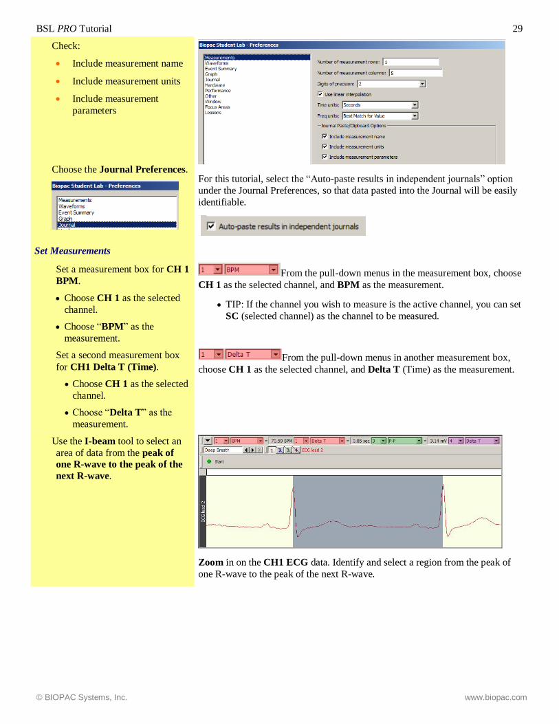
Use the I-beam tool to select an

area of data from the peak of

one R-wave to the peak of the

next R-wave.

Zoom in on the CH1 ECG data. Identify and select a region from the peak of

one R-wave to the peak of the next R-wave.


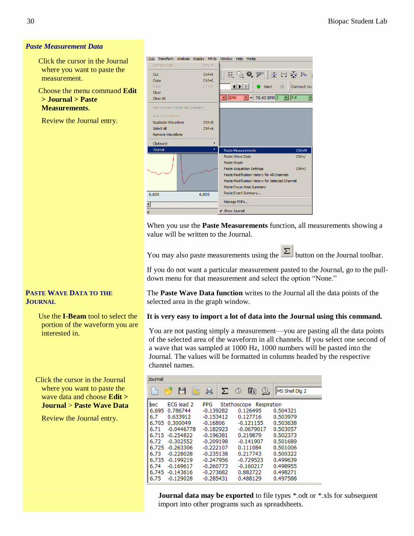
Paste Measurement Data

Click the cursor in the Journal

where you want to paste the

measurement.

Choose the menu command Edit

> Journal > Paste

Measurements.

Review the Journal entry.

When you use the Paste Measurements function, all measurements showing a

value will be written to the Journal.

You may also paste measurements using the button on the Journal toolbar.

If you do not want a particular measurement pasted to the Journal, go to the pull-

down menu for that measurement and select the option “None.”

PASTE WAVE DATA TO THE

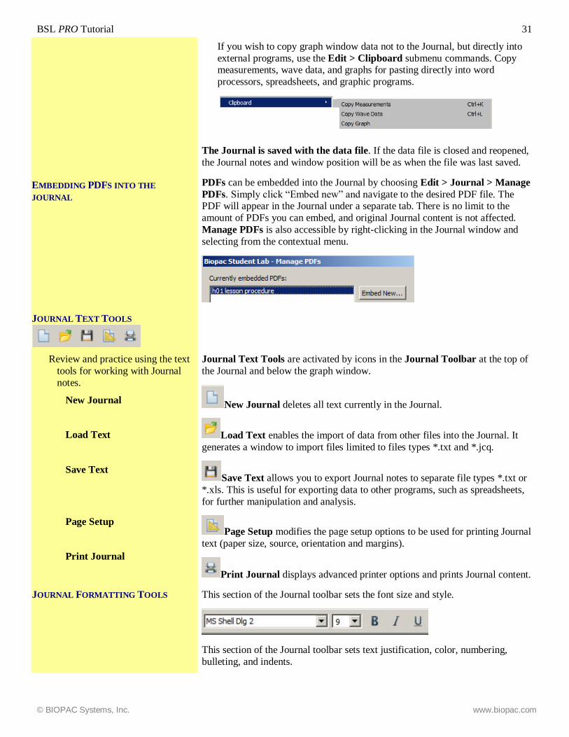
JOURNAL

The Paste Wave Data function writes to the Journal all the data points of the

selected area in the graph window.

Use the I-Beam tool to select the portion of the waveform you are

interested in.

It is very easy to import a lot of data into the Journal using this command.

You are not pasting simply a measurement—you are pasting all the data points

of the selected area of the waveform in all channels. If you select one second of a wave that was sampled at 1000 Hz, 1000 numbers will be pasted into the

Journal. The values will be formatted in columns headed by the respective

channel names.

Click the cursor in the Journal

where you want to paste the wave data and choose Edit >

Journal > Paste Wave Data

Review the Journal entry.

Journal data may be exported to file types *.odt or *.xls for subsequent

import into other programs such as spreadsheets.

BSL PRO Tutorial 31


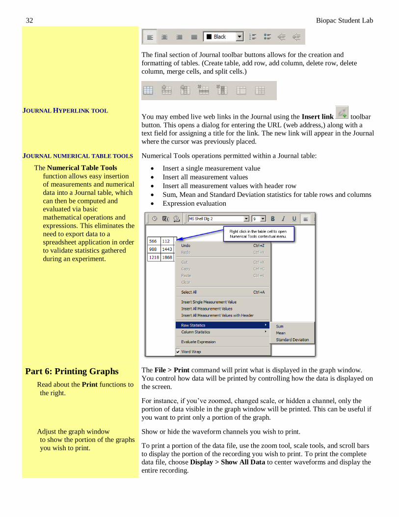
If you wish to copy graph window data not to the Journal, but directly into

external programs, use the Edit > Clipboard submenu commands. Copy measurements, wave data, and graphs for pasting directly into word

processors, spreadsheets, and graphic programs.

EMBEDDING PDFS INTO THE

JOURNAL

JOURNAL TEXT TOOLS

The Journal is saved with the data file. If the data file is closed and reopened,

the Journal notes and window position will be as when the file was last saved.

PDFs can be embedded into the Journal by choosing Edit > Journal > Manage

PDFs. Simply click “Embed new” and navigate to the desired PDF file. The PDF will appear in the Journal under a separate tab. There is no limit to the

amount of PDFs you can embed, and original Journal content is not affected.

Manage PDFs is also accessible by right-clicking in the Journal window and

selecting from the contextual menu.

Review and practice using the text

tools for working with Journal

notes.

New Journal

Load Text

Save Text

Page Setup

Print Journal

Journal Text Tools are activated by icons in the Journal Toolbar at the top of

the Journal and below the graph window.

New Journal deletes all text currently in the Journal.

Load Text enables the import of data from other files into the Journal. It

generates a window to import files limited to files types *.txt and *.jcq.

Save Text allows you to export Journal notes to separate file types *.txt or

*.xls. This is useful for exporting data to other programs, such as spreadsheets,

for further manipulation and analysis.

Page Setup modifies the page setup options to be used for printing Journal

text (paper size, source, orientation and margins).

Print Journal displays advanced printer options and prints Journal content.

JOURNAL FORMATTING TOOLS This section of the Journal toolbar sets the font size and style.

This section of the Journal toolbar sets text justification, color, numbering,

bulleting, and indents.


The final section of Journal toolbar buttons allows for the creation and

formatting of tables. (Create table, add row, add column, delete row, delete

column, merge cells, and split cells.)

JOURNAL HYPERLINK TOOL You may embed live web links in the Journal using the Insert link toolbar

button. This opens a dialog for entering the URL (web address,) along with a text field for assigning a title for the link. The new link will appear in the Journal

where the cursor was previously placed.

JOURNAL NUMERICAL TABLE TOOLS

The Numerical Table Tools

function allows easy insertion of measurements and numerical

data into a Journal table, which

can then be computed and evaluated via basic

mathematical operations and

expressions. This eliminates the

need to export data to a spreadsheet application in order

to validate statistics gathered

during an experiment.

Numerical Tools operations permitted within a Journal table:

• Insert a single measurement value

• Insert all measurement values

• Insert all measurement values with header row

• Sum, Mean and Standard Deviation statistics for table rows and columns

• Expression evaluation

Part 6: Printing Graphs

Read about the Print functions to

the right.

The File > Print command will print what is displayed in the graph window.

You control how data will be printed by controlling how the data is displayed on

the screen.

For instance, if you’ve zoomed, changed scale, or hidden a channel, only the

portion of data visible in the graph window will be printed. This can be useful if

you want to print only a portion of the graph.

Adjust the graph window to show the portion of the graphs

you wish to print.

Show or hide the waveform channels you wish to print.

To print a portion of the data file, use the zoom tool, scale tools, and scroll bars

to display the portion of the recording you wish to print. To print the complete data file, choose Display > Show All Data to center waveforms and display the

entire recording.

BSL PRO Tutorial 33


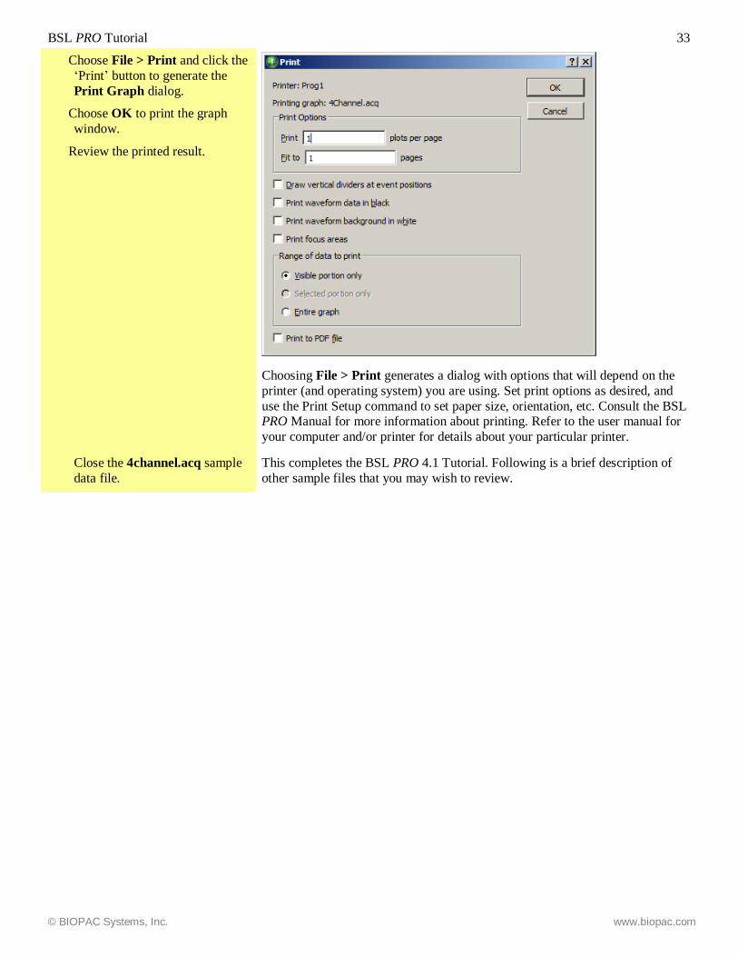
Choose File > Print and click the

‘Print’ button to generate the

Print Graph dialog.

Choose OK to print the graph

window.

Review the printed result.

Choosing File > Print generates a dialog with options that will depend on the

printer (and operating system) you are using. Set print options as desired, and

use the Print Setup command to set paper size, orientation, etc. Consult the BSL PRO Manual for more information about printing. Refer to the user manual for

your computer and/or printer for details about your particular printer.

Close the 4channel.acq sample

data file.

This completes the BSL PRO 4.1 Tutorial. Following is a brief description of

other sample files that you may wish to review.


Sample Data Files To further familiarize yourself with features of BSL PRO and see how it can

make your work easier, open and examine other data sample files included

with the BSL PRO installation. Sample files include the following.

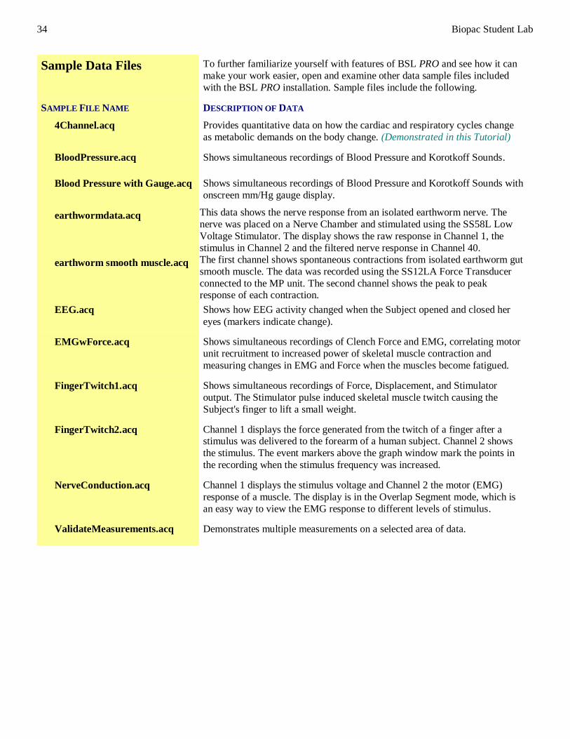
SAMPLE FILE NAME DESCRIPTION OF DATA

4Channel.acq Provides quantitative data on how the cardiac and respiratory cycles change

as metabolic demands on the body change. (Demonstrated in this Tutorial)

BloodPressure.acq Shows simultaneous recordings of Blood Pressure and Korotkoff Sounds.

Blood Pressure with Gauge.acq Shows simultaneous recordings of Blood Pressure and Korotkoff Sounds with

onscreen mm/Hg gauge display.

earthwormdata.acq This data shows the nerve response from an isolated earthworm nerve. The

nerve was placed on a Nerve Chamber and stimulated using the SS58L Low

Voltage Stimulator. The display shows the raw response in Channel 1, the

stimulus in Channel 2 and the filtered nerve response in Channel 40.

earthworm smooth muscle.acq The first channel shows spontaneous contractions from isolated earthworm gut

smooth muscle. The data was recorded using the SS12LA Force Transducer

connected to the MP unit. The second channel shows the peak to peak response of each contraction.

EEG.acq Shows how EEG activity changed when the Subject opened and closed her

eyes (markers indicate change).

EMGwForce.acq Shows simultaneous recordings of Clench Force and EMG, correlating motor

unit recruitment to increased power of skeletal muscle contraction and

measuring changes in EMG and Force when the muscles become fatigued.

FingerTwitch1.acq Shows simultaneous recordings of Force, Displacement, and Stimulator

output. The Stimulator pulse induced skeletal muscle twitch causing the

Subject's finger to lift a small weight.

FingerTwitch2.acq Channel 1 displays the force generated from the twitch of a finger after a stimulus was delivered to the forearm of a human subject. Channel 2 shows

the stimulus. The event markers above the graph window mark the points in

the recording when the stimulus frequency was increased.

NerveConduction.acq Channel 1 displays the stimulus voltage and Channel 2 the motor (EMG)

response of a muscle. The display is in the Overlap Segment mode, which is

an easy way to view the EMG response to different levels of stimulus.

ValidateMeasurements.acq Demonstrates multiple measurements on a selected area of data.

BSL PRO Tutorial 35


Sample Graph

Templates

The following sample graph templates (*.gtl files) are also included. Graph

templates contain no data, but are preset and ready to use for recording

various experiments, after which they can be saved as *.acq files.

BPM Gauge.gtl Heart Rate gauge window example. Displays ECG and Heart Rate (BPM) in the graph window and shows Heart Rate in a gauge window. It includes the

range band option, shaded red, to indicate Maximum Heart Rate range. To

change Gauge parameters, choose Preferences from right contextual menu

when the mouse is over the gauge window.

Heart Template.gtl Preset for ECG, Pulse and Heart Rate channels, with Input Values display.

Segment Timer Gauge.gtl Segment Timer gauge example. Records and displays ECG in the graph

window and a segment timer in the gauge window. The template is setup to

record ECG Lead II on CH 1, however no connections are needed to verify the

segment timer.

SS19L Gauge.gtl Setting up Gauge view for working with Blood Pressure Cuff Transducer

SS19L.

SS19LA Gauge.gtl Setting up Gauge view for working with Blood Pressure Cuff Transducer SS19LA.


Copyright

Information in this document is subject to change without notice and does not represent a commitment on the part of

BIOPAC Systems, Inc. This tutorial and the software it describes are copyrighted with all rights reserved. Under

copyright laws, this tutorial or the software may not be copied, in whole or part, without the written consent of BIOPAC

Systems, Inc., except in the normal use of the software or to make a backup copy.

The same proprietary and copyright notices must be affixed to any permitted copies as were affixed to the original. This

exception does not allow copies to be made for others, whether or not sold, but all of the material purchased (with all

backup copies) may be sold, given, or loaned to another person. Under the law, copying includes translating into another

language or format.

Biopac Student Lab Tutorial, including all text and graphics, are ©1998-2019 BIOPAC Systems, Inc., with all rights

reserved.

Limited Warranty

BIOPAC Systems, Inc. guarantees its equipment against all defects in materials and workmanship to the original

purchaser for a period of 12 months from the date of shipment unless otherwise stated below; effective 1-1-2015, BIOPAC MP36 units are guaranteed against defects in materials and workmanship to the original purchaser for a period

of 60 months (5 years) from the date of shipment.

If BIOPAC Systems, Inc. receives notice of such defects during the warranty period, BIOPAC Systems, Inc. will at its

option, either repair or replace the hardware products that prove to be defective in materials or workmanship. This warranty applies only if your BIOPAC Systems, Inc. product fails to function properly under normal use and within the

manufacturer’s specifications. This warranty does not apply if, in the sole opinion of BIOPAC Systems, Inc., your

BIOPAC Systems, Inc. product has been damaged by alteration, accident, abuse, misuse, neglect, improper packing, shipping, modification or servicing, by any party other than BIOPAC Systems, Inc. If a problem arises, please contact us

for authorization before returning an item.

Any returns should be supported by a Return Mail Authorization (RMA) number issued by BIOPAC Systems, Inc.

BIOPAC Systems, Inc. reserves the right to refuse to accept delivery of any shipment containing any shipping carton which does not have the RMA number(s) displayed on the outside. The Buyer will prepay transportation charges to the

BIOPAC Systems, Inc. designated site. The warranty period for repairs and for used equipment purchased from

BIOPAC is 90 days.

BIOPAC Systems, Inc. makes no other warranty or representation, either expressed or implied, with respect to any

hardware or software product, its quality, performance, merchantability, or fitness for a particular purpose.

BIOPAC Systems, Inc. will not be liable for direct, indirect, special, incidental, or consequential damages resulting from any defect in a hardware or software product or its documentation, even if advised of the possibility of such damages, or

for damage of any equipment connected to a BIOPAC Systems, Inc. product.

Trademarks

Biopac Student Lab is a trademark of BIOPAC Systems, Inc.

Windows is a trademark of Microsoft Corporation; Mac OS X is a trademark of Apple Computer, Inc.

This document was created with Microsoft Word for Windows, Adobe Photoshop, Adobe Distiller, Corel Draw 7.0,

Mainstay Capture, FastStone Capture and JASC, Inc. JasCapture.

Biopac Student Lab 4.1 BSL PRO TUTORIAL · 2 Biopac Student Lab Welcome to the Biopac Student Lab...

Documents

Transcript of Biopac Student Lab 4.1 BSL PRO TUTORIAL · 2 Biopac Student Lab Welcome to the Biopac Student Lab...