biomodeling with petri nets - Theseus

Bachelor’s Thesis

Degree Programme in Information Technology, International

Information Technology

2014

Romina Luciana Paturca

BIOMODELING WITH PETRI NETS

BACHELOR´S THESIS | ABSTRACT TURKU UNIVERSITY OF APPLIED SCIENCES

Information Technology | Internet Technology

13.01.2014 | 38

Instructor: Al-Bermanei Hazem

Romina Luciana Paturca

BIOMODELING WITH PETRI NETS

ABSTRACT

Petri nets are graphic-based modeling tools for systems where activity and

information flows have an important role among physical components and

activities. Since their introduction, about 50 years ago, Petri nets have been

applied in various areas such as computer architecture, software design,

workflow management, programming, databases, process modeling, diagnosis,

simulation, discrete process control, communication protocols, and yet even

further outside of computer science, for example, administration, theories of

communication, natural sciences. At the same time, nets have been modified and

theoretically investigated and they have increased the interest of computer

scientists in net theory. Petri nets have also been adjusted in biology and used

for modeling biological networks.

This thesis presents the basic notions of Petri nets and their use for modeling

and verification of systems. The thesis starts with an introduction and a brief

history of Petri nets. It continues with properties of Petri Nets, modeling and

analysis techniques, and it concludes with the analysis of a biological case study

with a Petri net model.

KEYWORDS:

Petri nets, mathematical model, model validation, heat shock response, P-invariants, T-invariants.

ACKNOWLEDGMENTS

I would like to express my thanks of deep gratitude to my supervisor teacher Al-

Bermanei Hazem from Turku University of Applied Sciences for his guidance,

suggestions and constant encouragement throughout the course of this thesis as

well as Professor Ion Petre from Åbo Akademi University who gave me the

opportunity to do this project on the topic of “Biomodeling with Petri Nets”.

I would also like to thank to PhD candidate Diana-Elena Gratie for her continuous

and instant help offered to me throughout the process of this thesis.

CONTENTS

LIST OF ABBREVIATIONS 3

1 INTRODUCTION 4

2 BASIC NOTIONS AND FORMAL DEFINITIONS 6

2.1 Definitions of Graph Theory 6

2.2 Description of Standard Petri Nets 7

2.3 Enabling and firing rules 10

3 BASIC PROPERTIES OF PETRI NETS 12

3.1 Behavioral Properties 13

3.2 Structural Properties 14

4 MODELING AND ANALYSING WITH PETRI NETS 16

4.1 Biomodeling with Petri Nets 19

4.2 Snoopy and Charlie modeling tools 21

5 MODELING OF THE HEAT SHOCK RESPONSE WITH PETRI NETS 22

5.1 The Heat Shock Response 22

5.2 Molecular Model for the Heat Shock Response 23

5.3 Petri Net Model for the Heat Shock Response 25

6 CONCLUSION 32

REFERENCES 33

2.2.1 Formal Definition of a Petri Net (PN) 9

1

LIST OF FIGURES

FIGURE 1. A bipartite graph 6

FIGURE 2. Graphical representation of places, transitions, and arcs 8

FIGURE 3. Example of a Petri net 9

FIGURE 4. Example of a firing transition 11

FIGURE 5. A state machine and an event graph 12

FIGURE 6. Modeling cycle 17

FIGURE 7. A Petri net with corresponding reachability graph

and reachability tree 18

FIGURE 8. DNA binding activity at 42° C 27

FIGURE 9. Petri net model for HSR containing the first 9 reactions

of the system 30

FIGURE 10. Petri net model for HSR containing reactions 10, 11, 12

of the system 31

2

LIST OF TABLES

TABLE 1. Petri nets properties and their biological significance 20

TABLE 2. Species of HSR molecular model 23

TABLE 3. Reactions of HSR molecular model 24

TABLE 4. Reaction parameters 25

TABLE 5. Initial concentrations of species 26

TABLE 6. The P-invariants for the HSR reported by Charlie 28

TABLE 7. The T-invariants for the HSR reported by Charlie 29

3

LIST OF ABBREVIATIONS

PN Petri Nets

P-invariants Places invariants

T-invariants Transitions invariants

HSR Heat Shock Response

hsp heat shock protein

mfp misfolded protein

prot protein

hsf heat shock factor

hse heat shock element

4

TURKU UNIVERSITY OF APPLIED SCIENCES THESIS | Romina Luciana Paturca

1 INTRODUCTION

A Petri net is a language of nets that is favorable for the representation, in a

natural way, of logical interactions between activities and parts in a system

that holds characteristics like concurrency, synchronization, sequentiality, and

conflict. Petri nets can be used for graphical representation, as a visual

communication tool like block diagrams, flow charts, logical trees.

Historically, the theory of Petri nets has its origins in the doctoral thesis of C.A.

Petri submitted in 1962. It is stated in some sources that the theory was

invented in 1939, for describing chemical processes, by the 13-year old Carl

Adam Petri. Since then, Petri nets have been developed and used in both

theory and practice, providing a strong means of communication between

theoreticians and practitioners.

Petri nets have the ability to generalize the theory for process analysis by their

high expression in competitive events.

A Petri net is identified as a bipartite directed graph whose nodes are places

and transitions. Places represent conditions and transitions represent events.

An event has a particular number of input and output conditions representing

the pre-conditions and the post-conditions. In contrast with condition/event

nets, place/transition nets can hold any number of conditions (tokens).

Illustratively, places are depicted as circles, and transitions as boxes or bars.

Each arc of this graph connects a place and a transition. If there is an oriented

arc from a place towards a transition, then the place represents the point of

entry for the transition; conversely, if the arc is oriented from the transition to

the place, then the place represents the point of exit for the transition. Places

may contain a variable number of tokens, and their entire distribution over the

places of the net, represents the marking. Transitions occur by consuming the

input tokens and producing them into the output tokens.

The execution of a Petri net is a nondeterministic process. During the

execution, the active transitions are analyzed at each step. A transition is

active at the moment when every entry point contains at least one token.

5


The execution of a transition occurs by eliminating one token from each input

place and by adding one token to each output place. Only one transition can

be executed at a certain step.

This thesis is organized as follows. Chapter two contains basic notions of

graph theory and introduces Standard Petri nets. Chapter three presents the

behavioral and structural properties of Petri nets. Chapter four discusses a

couple modeling and analyzing methods of the formalism. Chapter five

contains the basic information about the Heat Shock Response and the

modeling of the Heat Shock Response with Petri nets.

6


2 BASIC NOTIONS AND FORMAL DEFINITIONS

2.1 Definitions of Graph Theory

Definition 2.1.1 A graph G = (V,E) consists of a set V of vertices (nodes) and a

set E of edges (lines).

Definition 2.1.2 A directed graph is a graph with directed edges. An undirected

graph is a graph in which edges have no direction.

Definition 2.1.3 A simple graph is an undirected graph which has no loops

(edges which start and end on the same vertex). A multigraph is a graph with

multiple edges.

Definition 2.1.4 A weighted graph (network) is a graph is which each edge has

a weight (real number).

Definition 2.1.5 A bipartite graph is a graph in which vertices can be divided

into two sets such that each edge connects one vertex in one set to one vertex

in the other set.

Figure 1. A bipartite graph

7


2.2 Description of Standard Petri Nets

A Petri net can be identified with a particular kind of bipartite directed graphs

populated with four types of objects. These objects are places, transitions,

directed arcs connecting places to transitions or transitions to places, and

tokens. Graphically, places are represented by circles and transitions by bars or

rectangular shapes. A place is an input to a transition if there is a directed arc

from the place to the transition. A place is an output for a transition if there is a

directed arc from the transition to the place. In its simplest form, a Petri net can

be represented by a transition with its input and output places. This basic

network can be used to represent different aspects of modeled systems. For

example, input / output places may represent preconditions / postconditions and

transitions may represent events. Inputs may signify the availability of

resources, transition their use, and outputs may signify the release of

resources.

Petri nets were designed to represent discrete and concurrent processes of

technical systems, but they also offer a simple and flexible modeling language

and they are useful in modeling biological systems being very efficient in

reconstructing molecular networks.

Places are inactive nodes that refer to conditions or states. They are visualized

by circles and in a biological context, they may signify: organisms, populations,

species, cells, proteins, molecules, and they may also represent temperature or

pH value as well as membrane potential.

Tokens are floating elements carried by places. Graphically, tokens are

represented by dots and they indicate the discrete value of a condition, and in

biological systems, they express discrete numbers of populations, species,

concentration levels, pH values, and temperatures.

Transitions are active nodes that consume and produce tokens. They may

represent different events and activities and, in a biological context, reactions,

interactions, and intramolecular changes.

8


Directed arcs, represented by arrows, may define products of a reaction,

reactants, determine the relationship between transitions and places, and show

the changes that occur in the marking. (Blätke 2011, p. 5-6).

Figure 2. Graphical representation of places, transitions, and arcs

9


2.2.1 Formal Definition of a Petri Net (PN)

A Petri Net is a 5-tuple where:

is a finite set of places

is a finite set of transitions

is a set of arcs

is a weight function

is the initial marking

and

(Murata 1989)

Figure 3. A Petri net with , and 0

10


2.3 Enabling and firing rules

The dynamic evolution of the PN marking is ruled by transition firings which

destroy and create tokens. Both the enabling and firing rules are specified

through arcs and they are associated with transitions so that the enabling rule

states the conditions under which transitions are allowed to fire and the firing

rule defines the marking modification or the change of state produced by the

transition.

Each place may contain a number of tokens. The transition is achieved only

when all places situated on a higher position contain at least one token. At a

certain moment, only one transition may occur by deleting and adding tokens. A

transition can start when each of the places connected to it, has at least one

token. When a transition is triggered, it removes the token from each input place

and adds one to each place connected to it. Moving tokens between places

takes place according to the firing rules imposed by transitions. Sometimes it is

necessary for an input place to contain two or more tokens before the transition

can start, and in this case, to avoid drawing more than one arc between place

and transition, the multiplicity of arcs is denoted by a number next to the arc.

Definition 2.3.1 A transition is said to be enabled if each upstream place

contains at least one token.

When transition t fires, it deletes from each place in its input set (preplaces of

transition t) as many tokens as the multiplicity of the arc connecting that place

to t, and adds to each place in its output set (postplaces of transition t) as

many tokens as the multiplicity of the arc connecting t to that place.

Definition 2.3.2 A firing of an enabled transition removes one token from each

of its upstream (input) places and adds one token to each of its downstream

(output) places.

The firing of transition t, enabled in marking produces marking such that

11


This statement is indicated as and is said that is directly reachable

from M. (Blätke 2011, p. 7-8).

Figure 4. A firing transition. The marking before firing transition t1 . The marking

after firing t1.

12


3 BASIC PROPERTIES OF PETRI NETS

With Petri net models two types of properties can be studied: properties which

depend on the initial marking and they are called behavioral properties, and

properties which are independent of the initial marking and they are known as

structural properties.

Before presenting the behavioral and structural properties, two features of Petri

nets will be introduced: event graph and state machine.

Definition 3.1 A Petri net is called an event graph if each place has exactly one

upstream and one downstream transition.

Definition 3.2 A Petri net is called a state machine if each transition has exactly

one upstream and one downstream place.

In an event graph, a token can be consumed by only one transition and several

places can come before a given transition. They can model synchronization and

may be referred to as marked graphs or decision free Petri nets.

A state machine can model competition and does not allow synchronization.

State machines have constant number of tokens and are referred to as strictly

conservative. (Baccelli et al. 2001, p. 59)

Figure 5. A state machine and an event graph (Source: Synchronization and Linearity, Baccelli et al. 2001, pp.59)

13


3.1 Behavioral Properties

1. Reachability is the fundamental base for studying the dynamic

properties of any system. The firing of the enabled transition will

change the token distribution, and the sequence of firings issues the

sequence of markings. A sequence of firings is denoted by

σ = M0 t1 M1 t2 tn Mn or σ t1 t2 tn

The marking is reachable from the initial marking if there exists

a firing sequence that transforms into and in this case, is said

that Mn is reachable from by σ, and is indicated as . By

or is denoted the set of all possible markings

reachable from in a net , and by or is

denoted the set of all possible firing sequences from in a net

.

2. Liveness is related to potential fireability in all reachable markings. A

transition is live if it is potentially firable in any marking, and it is dead,

if it is not potentially firable. Deadlock-freeness is a weaker condition in

which fireability of the net system is guaranteed, but some parts of it

may not work at all.

3. Safeness. A Petri net is safe if the number of tokens in each place is

not greater than 1 in any marking.

4. Boundedness characterizes the finiteness of the state space and it is a

simple generalization of safeness. A Petri net is bounded if the token

count in each place is less or equal to (a finite number) for every

marking reachable from the initial marking.

5. Reversibility characterizes recoverability of the initial marking from any

reachable marking. In some cases, it is not necessary to get back to

the initial marking as long as one can get back to some marking. In

that case, the marking is called Home State.

14


6. Conservation. A Petri net is strictly conservative if the token count is

constant in each marking.

7. Coverability. A marking is coverable from if there exists a

marking such that for all places p in the

net.

8. Persistance. A Petri net is persistent if the firing of one transition from

two enabled ones will not disable the other transition. In a persistent

net, an enabled transition will remain enabled until it fires.

9. Fairness. The literature on Petri nets are proposes different notions of

fairness. Here is presented one basic concept: bounded-fairness. A

Petri net is a bounded-fair (B-fair) net if each pair of transitions in the

net is in a B-fair relation; and for two transitions to be in a B-fair

relation, the maximum number of times, that either one can fire, has to

be bounded while the other transition is not firing.

3.2 Structural Properties

Whereas the behavioral properties of Petri nets are dependent on the initial

marking and the firing rule, the structural properties depend only on the

topological structure of Petri nets. These structural properties have a high

significance in the designing of manufacturing systems, as they are dependent

just on the layout, and not on the manner the system will be managed, a fact

that is not known at the design level. The structural properties of Petri nets

include liveness, boundedness, consistency, repetitivity, conservativeness, and

controllability properties, and most of them can be verified by means of

algebraic techniques.

1. Structural Liveness. A Petri net is structurally live if there exists a live

initial marking.

15


2. Boundedness. A Petri net is structurally bounded if it is bounded for

any finite initial marking.

3. Consistency. A Petri net is consistent if there exists an initial marking

and a firing sequence from the initial marking back to the initial

marking such that each transition occurs at least one in the firing

sequence.

4. Repetitivity. A Petri net is repetitive if there exists an initial marking

and a firing sequence from the initial marking such that each transition

occurs unlimitedly in the firing sequence.

5. Conservativeness. A Petri net is conservative if all transitions add

exactly as many tokens to their output places as they subtract from

their input places.

6. Controllability. A Petri net is completely controllable if either marking is

reachable from any other marking.

16


4 MODELING AND ANALYSING WITH PETRI NETS

A model represents a partial conception of the reality and the description of its

main features and the connections among them. Many models may be given for

a certain object of study and each of them may be focusing on different features

of the given object. Computational modeling is a mathematical representation of

the reality, and computational models simulate the reality by using the language

of mathematics.

The starting point for modeling is represented by the following selection:

Features whose effects are neglected and they will be ignored in the

model.

Features that affect the model but their behavior will not be studied in the

model and they will be represented as inputs, parameters, external or

independent variables of the model.

Features that the model is focusing on, and they will represent the

internal or dependent variables of the model.

The validation of models is checked by comparison to experimental data and as

result models can be invalidated. Models are not certain, are not the reality, and

their validation cannot be absolutely confirmed by experimental data. (Petre

2013).

17


Simplification

Verification Analysis

Interpretation

Figure 6. Modeling cycle (Petre 2013)

Petri nets were designed for and are used particularly for modeling. Petri nets

are used to model systems with independent components, the occurrence of

different activities and events in a system, and the flow of information or other

resources within a system. The systems may be of numerous various kinds:

computer hardware, computer software, computer networks, real-time

computing systems, communication systems, logistic networks, manufacturing

plants, physical systems, social systems, biological systems, and so on.

Petri nets compound a mathematical theory with a graphical representation of

the dynamic behavior of a system.

Some of the methods used for modeling and analyzing systems with Petri nets

are the reachability tree and incidence matrix.

Definition 4.1 (Reachability tree) The reachability tree of a Petri net is a

tree with nodes in which is obtained as follows: the initial marking μ is a

node of this tree; for each enabled in , the marking obtained by firing is a

new node of the reachability tree; arcs connect nodes which are reachable from

one another in one step; this process is applied recursively from each such .

(Baccelli et al. 2001, pp. 57)

Real-world data & hypothesis

Predictions / explanations

Mathematical conclusions

Model

18


Definition 4.2 (Reachability graph) The reachability graph is obtained from the

reachability tree by merging all nodes corresponding to the same marking into a

single node. (Baccelli et al. 2001, pp. 57)

The following example shows a Petri net with both transitions enabled and an

initial marking . If transition is the first to fire, the next marking

becomes . In case that fires first, the marking will be .

Starting from , only can fire and leads to the initial marking, and

from , by firing , only the initial marking can be reached. The

reachability graph of has three different markings.

Figure 7. A Petri net with corresponding reachability graph and reachability tree (Source: Synchronization and Linearity, Baccelli et al. 2001, pp. 58)

19


An alternative method for representation and analysis of Petri nets is based on

matrix equations used to represent the dynamic behavior of Petri nets. The

method involves constructing the incidence matrix that defines all possible

interconnections between places and transitions. The incidence matrix of a Petri

net is an matrix, where is the number of transitions and is the

number of places.

4.1 Biomodeling with Petri Nets

Biological systems consist of species and the interactions among them. Some

interactions can be independent and could fire in parallel. The characteristics of

biological systems of being bipartite and having concurrent behavior make them

suitable for modeling with Petri nets. The advantage of using Petri nets for

modeling biological systems lies in the ability of analyzing both structural and

behavioral properties of the system. Two important properties of PN met while

modeling biological systems are the places and transitions invariants (P- and T-

invariants). P-invariants are sets of places with constant weighted sum of

tokens and they correspond to mass conservation relations. T-invariants are

sets of transitions whose ordered firing reproduces the initial state and they

correspond to elementary modes of a system.

A reaction-based biological network is formed out of a set of reactions with the

following general form , where

species represent the substrate of the reaction and species

represent the products of the reaction.

Within the Petri nets formalism, species are modeled as places and reactions

as transitions having substrates as pre-places and products as post-places.

(Gratie & Petre 2013).

20


The following table presents some of the properties of Petri nets and their

biological significance.

Table 1. Petri nets properties and their biological significance

𝑫

𝑤

𝑫

𝑯 𝒎

𝐸

𝑪

21


4.2 Snoopy and Charlie modeling tools

Snoopy is a software tool designed for modeling and running Petri nets. It

supports standard PN as well as many extensions of the formalism. Snoopy

provides different shapes for net elements, coloring of graph elements,

animation and simulation of PN, exporting and importing to and from different

file types.

For analyzing a model, Snoopy offers support for Charlie. Charlie is a software

tool designed for analyzing structural and behavioral properties of PN and is

used for the verification of different systems and the validation of natural

systems.

For the case study presented in this thesis, the last versions of Snoopy (2013-

07-30) and Charlie (2013-05-13) will be used.

22


5 MODELING OF THE HEAT SHOCK RESPONSE WITH

PETRI NETS

5.1 The Heat Shock Response

The heat shock response (HSR) is a highly conserved regulatory mechanism

that allows the cell to quickly react to elevated temperatures and stress

conditions. A heat shock is produced by the exposure of a cell to a temperature

greater than its optimum. The equilibrium in an over-heated cell is recovered by

the heat shock response that diminishes the shock effects through the activity of

specialized proteins. Exposed to high temperatures, proteins misfold and tend

to form large aggregates with killing effects on the cell leading to programmed

cell death. Opposing this, cells produce heat shock proteins (hsps) with the role

of assisting misfolding proteins (mfps) in their correct refolding.

The heat shock response has been the subject of active research in the past

decades, as the hsps play a major role in many biological processes. Thus,

understanding the mechanism of HSR has fundamental importance for the

biology of the cell as well as response to cellular affronts and treatment of

certain diseases.

In this thesis, for our Petri net model, we consider the basic molecular model for

the heat shock response proposed in the research paper “A simple mass-action

model for the eukaryotic heat shock response and its mathematical validation.”

(Petre et al. 2011).

23


5.2 Molecular Model for the Heat Shock Response

Through the course of the heat shock response, the heat shock factors (hsfs),

also called monomers, form active components known as trimers, which bind to

heat shock elements (hses). This bind leads to the appearance of heat shock

proteins. The presence of sufficient amounts of hsp contributes to unbinding

trimers from hse and separates them into monomers. Hsps facilitate the

refolding of misfolding proteins.

The molecular model considered in this paper contains 10 species and 12

reactions, as proposed in the publication mentioned above.

The species are listed in Table 2, and following simplifications have been done:

all types of heat shock proteins are treated as one species (hsp), all types of

heat shock factors are also treated as one species (hsf), the aspect of proteins

taken into account for the modeling process is the folding of proteins: correct

folded (prot) or misfolded proteins (mfp).

The species of the basic molecular model for HSR are shown in Table 2.

Table 2. Species of HSR molecular model

𝒎

24


The reactions of the model for the heat shock response are presented in Table

3. Reactions 1 and 2 contain the dimerization and trimerization of heat shock

factors; in reaction 3 trimers bind to heat shock elements; reaction 4 covers the

generation of new heat shock proteins; in reactions 5-8, heat shock proteins

contribute to the unbinding of heat shock factors, dimers (hsf2) and trimers

(hsf3); with reaction 9 is represented the degradation of heat shock proteins;

reactions 10-12 cover the protein misfolding and folding activities.

Table 3 presents the list of reactions in the molecular model for the heat shock

response.

Table 3. Reactions of HSR molecular model

𝒎

2

2

25


5.3 Petri Net Model for the Heat Shock Response

The Petri net model of the heat shock response molecular model can be seen in

Figures 9 and 10. In order to be able to validate our model, the numerical setup,

the reaction parameters and the initial concentrations of species are consistent

with the values reported in “A simple mass-action model for the eukaryotic heat

shock response and its mathematical validation” publication and presented in

the following tables:

Table 4. Reaction parameters

𝒎

𝑤

𝑤

𝑤

𝑤 -9

𝑤

𝑤 -6

-3

𝑤

𝑤

-5

-7

-5

-5

𝑤 -3

𝑤

26


Table 5. Initial concentrations of species

𝑪

-4

-4

8

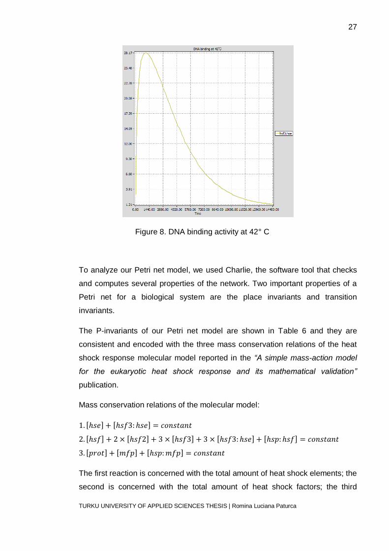
To be able to compare the predictions of our study case with Snoopy

implementation, the simulation time was 14400s, and the results are consistent

as those reported in the publication. At 37° C, when no regulatory activities

occur, the model is considered to be in a steady state. At 42° C, hsf3s bind to

hses located on DNA strands and promote replication of heat shock genes.

Hsps assist the correct folding of misfolding proteins and they react with hsf3’s

breaking bounds of hsf3:hse. Eventually, the concentration of DNA binding

activity returns to basal level. Figure 8 illustrates the DNA binding activity of our

model at 42° C.

27


Figure 8. DNA binding activity at 42° C

To analyze our Petri net model, we used Charlie, the software tool that checks

and computes several properties of the network. Two important properties of a

Petri net for a biological system are the place invariants and transition

invariants.

The P-invariants of our Petri net model are shown in Table 6 and they are

consistent and encoded with the three mass conservation relations of the heat

shock response molecular model reported in the “A simple mass-action model

for the eukaryotic heat shock response and its mathematical validation”

publication.

Mass conservation relations of the molecular model:

] ]

] ] ] ] ]

] ] ]

The first reaction is concerned with the total amount of heat shock elements; the

second is concerned with the total amount of heat shock factors; the third

28


reaction is concerned with the total amount of proteins. The amounts of heat

shock elements, heat shock factors and proteins are constant in a cell.

Table 6. The P-invariants for the HSR reported by Charlie

The model being covered with P-invariants, also suggests that the Petri net is

structurally bounded and conservative.

Table 7 illustrates the T-invariants of our model. They all validate the model in

the sense that all successions of reactions that balance each other out, are

present in a t-invariant. For example, the T-invariant 9 denotes the sequence of

reactions needed in order to first produce and then consume one token of

misfolded protein. Being covered by T-invariants, the net is repetitive and

consistent.

The reachability graph property checked with Charlie, indicated that the

reachability graph of the net contains one single place, meaning that all places

are interconnected and from each place it can be reach any other one by

following successive arcs.

𝒎 𝑪 𝒎

29


Table 7. The T-invariants for the HSR reported by Charlie

𝒎

𝑤

𝑤

𝑤

𝑤

𝑤

𝑤

𝑤

𝑤

𝑤

𝑤

𝑤

𝑤

𝑤

𝑤

𝑤

𝑤

𝑤

𝑤

𝑤

𝑤

30


Figure 9. Petri net model for HSR containing the first 9 reactions of the

molecular model

31


Figure 10. Petri net model for HSR containing reactions 10, 11, 12 of the

molecular model

For a better visualization and clarity of the model, transitions (reactions in

molecular model) and their corresponding arcs are depicted with different

colors. The species of the molecular model represent the variables in the Petri

net model, and graphically, they are indicated as circles containing their initial

values (concentrations). To avoid the overlapping of arcs where possible, some

species involved in more than one reaction, repeat in the model and they are

indicated by grey filled places.

32


6 CONCLUSION

This thesis offered a brief introduction to Petri nets and their applications. Since

their introduction, Petri nets have been modified and theoretically investigated

and applied to a vast number of areas. Their research touched not only on

various aspects of computer science and mathematics, but on natural sciences

as well, representing a favorable mean for modeling and analyzing biological

systems.

Modeling with Petri nets permits structural and behavioral analysis of modeled

systems. In our Petri net model for the Heat Shock Response, we studied, in

principle, the place invariants and transition invariants, and the model showed

that they are similar with reported biological data.

Modeling and analyzing biology systems are significant for a better

understanding of biology by reconstructing rules underlying biological systems,

as well as for medical diagnosis and therapeutic suggestions.

33


REFERENCES

Baccelli, F., Cohen, G., Olsder, G.J. & Quadrat, J.P. 2001, Synchronization and Linearity, E-book, pp. 35-97.

Behavioral & structural properties, Lecture notes available at <http://brahms.emu.edu.tr/rza/isys501week3.pdf>. Consulted 16.07.2013.

Blätke, 2011. Tutorial: Petri Nets in Systems Biology, 1st Ed. Available at <http://www.regulationsbiologie.de/pdf/BlaetkeTutorial.pdf>. Consulted 17.06.2013.

Charlie Software Tool, Available at <http://www-dssz.informatik.tu-cottbus.de/DSSZ/Software/Charlie>.

Girault, C & Valk, R. 2001, Petri Nets for Systems Engineering, Berlin, Springer.

Gratie, D., Petre, I. 2013. Quantitative Petri Net Models for the Heat Shock Response, TUCS Technical Report, No. 1068. Also available at <http://combio.abo.fi/publications-2/>. Consulted 26.11.2013.

Introduction & formal definitions, Lecture notes available at <http://brahms.emu.edu.tr/rza/isys501week1.pdf>. Consulted 16.07.2013.

Marsan, A., Balbo, Conte, Donatelli, & Franceschinis 1995, Modelling with generalized stochastic petri nets, Chichester, John Wiley.

Murata, T. 1989. “Petri Nets: Properties, Analysis and Applications”, Proceedings of the IEEE, vol. 77, no. 4, pp. 541-567. Available at <http://embedded.eecs.berkeley.edu/Research/hsc/class.F03/ee249/discussionpapers/PetriNets.pdf>. Consulted 18.06.2013.

Peterson, L. J. 1981, Petri Net Theory And The Modeling Of Systems, Englewood Cliffs, N.J., Prentice-Hall.

Petre 2013, Building and analyzing a computational biomodel, Lecture notes distributed in Introduction to computational and systems biology at Åbo Akademi University Finland, Turku on 9 October 2013. Available at <http://users.abo.fi/ipetre/compsysbio/Lecture_12.pdf>. Consulted 9.10.2013.

http://brahms.emu.edu.tr/rza/isys501week3.pdf

http://www.regulationsbiologie.de/pdf/BlaetkeTutorial.pdf

http://www-dssz.informatik.tu-cottbus.de/DSSZ/Software/Charlie

http://www-dssz.informatik.tu-cottbus.de/DSSZ/Software/Charlie

http://combio.abo.fi/www_includes/pub_details.php?id=693

http://combio.abo.fi/www_includes/pub_details.php?id=693

http://brahms.emu.edu.tr/rza/isys501week1.pdf

34


Petre 2012, Modeling with Petri nets, Lecture notes distributed in Advanced computational modeling at Åbo Akademi University Finland, Turku on 5 December 2012. Available at <http://users.abo.fi/ipetre/advcompmod/>. Consulted 22.11.2013.

Petre, I., Mizera, A., Hyder, C.L., Meinander, A., Mikhailov, A., Morimoto, R.I., Sistonen, L., Eriksson, J.E. & Back, R.J. 2011, “A simple mass-action model for the eukaryotic heat shock response and its mathematical validation.” Natural Computing Vol. 10, Issue 1, pp. 595-612.

Snoopy Software Tool, Available at <http://www-dssz.informatik.tu-cottbus.de/DSSZ/Software/Snoopy>.

http://users.abo.fi/ipetre/advcompmod/

http://www-dssz.informatik.tu-cottbus.de/DSSZ/Software/Snoopy

http://www-dssz.informatik.tu-cottbus.de/DSSZ/Software/Snoopy

biomodeling with petri nets - Theseus

Documents

Transcript of biomodeling with petri nets - Theseus