Biome BGC version 4.2: Theoretical Framework of Biome-BGC ...€¦ · Biome BGC version 4.2:...
71
1 Biome BGC version 4.2: Theoretical Framework of Biome-BGC January, 2010 Abstract : BiomeBGC (BBGC) is a mechanistic model that is used to estimate the state and fluxes of carbon (C), nitrogen (N), and water (H 2 O) into and out of an ecosystem. BBGC is actively used in institutions around the globe and its most recent release is version 4.2. As mentioned above, the 3 primary biogeochemical cycles represented in BBGC are the C, N, and H 2 O cycles. In conjunction with these cycles, BBGC models the physical processes of radiation and water disposition. BBGC partitions incoming radiation and precipitation and treats the excess/unused portions as outflows. The primary physiological processes modeled by BBGC are photosynthesis, evapotranspiration, respiration (autotrophic and heterotrophic), decomposition, the final allocation of photosynthetic assimilate, and mortality. To model these processes, BBGC first models the phenology of the systems based on the input meteorological data. This description of BBGC below will attempt to follow the order and structure of BBGC as it is implemented to best represent the flow of information through the model system. A general discussion of the model flow and required inputs will be given first, followed by a broad outline of the model processes and assumptions. BBGC will be compared to Forest Gap Models and Growth and Yield Models. Lastly, a detailed description of each of the BBGC’s processes will be presented (Peter Thornton’s thesis was an essential reference in understanding this model (Thornton 1998)).
Transcript of Biome BGC version 4.2: Theoretical Framework of Biome-BGC ...€¦ · Biome BGC version 4.2:...

1
Biome BGC version 4.2: Theoretical Framework of Biome-BGC
January, 2010
Abstract:
BiomeBGC (BBGC) is a mechanistic model that is used to estimate the state and fluxes
of carbon (C), nitrogen (N), and water (H2O) into and out of an ecosystem. BBGC is actively
used in institutions around the globe and its most recent release is version 4.2. As mentioned
above, the 3 primary biogeochemical cycles represented in BBGC are the C, N, and H2O cycles.
In conjunction with these cycles, BBGC models the physical processes of radiation and water
disposition. BBGC partitions incoming radiation and precipitation and treats the excess/unused
portions as outflows. The primary physiological processes modeled by BBGC are
photosynthesis, evapotranspiration, respiration (autotrophic and heterotrophic), decomposition,
the final allocation of photosynthetic assimilate, and mortality. To model these processes,
BBGC first models the phenology of the systems based on the input meteorological data.
This description of BBGC below will attempt to follow the order and structure of BBGC
as it is implemented to best represent the flow of information through the model system. A
general discussion of the model flow and required inputs will be given first, followed by a broad
outline of the model processes and assumptions. BBGC will be compared to Forest Gap Models
and Growth and Yield Models. Lastly, a detailed description of each of the BBGC’s processes
will be presented (Peter Thornton’s thesis was an essential reference in understanding this model
(Thornton 1998)).

2
Table of Contents Section 1: General Model Flow................................................................................................... 3 Section 2: Model Overview.......................................................................................................... 4
Broad Conceptual Basis and Critical Assumptions:................................................................... 4 Physical Model Processes ............................................................................................................ 6
Radiation: .................................................................................................................................. 6 Precipitation and H2O Cycle: ................................................................................................... 8
Physiological Model Processes: C and N Cycle – Pools and Fluxes ........................................ 9 Maintenance Respiration: ....................................................................................................... 11 Photosynthesis:........................................................................................................................ 11 Decomposition: ....................................................................................................................... 11 Allocation: ............................................................................................................................... 13 Growth Respiration:................................................................................................................ 14 Mortality: ................................................................................................................................ 14
Principle of the Conservation of Energy and Mass: ................................................................. 14 Section 3: Comparison of BBGC with Gap Models and Growth and Yield Models ........... 14
Forest Gap Models: .................................................................................................................... 16 Forest Growth and Yield Models:.............................................................................................. 18
Section 4: BiomeBGC – Utility and Applications ................................................................... 20 Section 5: Detailed Model Description ..................................................................................... 22
Precalculations:.......................................................................................................................... 22 Prephenology (prephenology.c):................................................................................................ 24 Daily Meteorology and Soil Temperature (daymet.c): .............................................................. 26 Apply Prephenology to Daily Fluxes (phenology.c): ................................................................ 26 Partition Leaf C into Sun and Shade LAI and Partition Incoming Radiation (radtrans.c): .. 27 Precipitation Routing (prcp_route.c): ....................................................................................... 28 Snow Water (snow_melt.c:) ....................................................................................................... 28 Penman-Monteith Equation (within canopy_et.c): .................................................................. 29 Soil Water Evaporation (baresoil_evap.c):................................................................................ 33 Soil Matric Potential (soilpsi.c): ................................................................................................ 34 Maintenance Respiration (maint_resp.c):................................................................................. 34 Canopy Evapotranspiration (canopy_et.c):............................................................................... 35 Photosynthesis (photosynthesis.c): ............................................................................................ 38 N Deposition and Fixation (within bgc.c):................................................................................ 44 H2O outflow (outflow.c): ............................................................................................................ 44 Decomposition (decomp.c):........................................................................................................ 45 Allocation (daily_allocation.c):.................................................................................................. 48 Growth Respiration (growth_resp.c): ........................................................................................ 51 Update C, N, and H2O state (state_update.c): ........................................................................... 51 N Leaching (nleaching.c): ......................................................................................................... 51 Mortality (mortality.c): ............................................................................................................... 51 Mass Balance Check (check_balance.c): .................................................................................. 52
Appendix A: Required BiomeBGC Inputs .............................................................................. 54 Appendix B: BiomeBGC Output Map (taken from output_map_init.c) .............................. 57 Appendix C: BBGC Constants (from bgc_constants.h) ......................................................... 66 References .................................................................................................................................... 67

3
Section 1: General Model Flow
Figure 1 shows the general flow of the BBGC model. The first step in any BBGC model
run is a spinup to bring the model into equilibrium. It is common for ecosystem models to
require a steady state initial condition so as to insure that there is a balance between input and
output fluxes and that the system has equilibrated to the environmental and site forcings
(Thornton and Rosenbloom 2005). In the current version of BBGC, this means that the
difference between the annual average daily soil carbon stocks must be less than a specified
spinup tolerance value (SPINUP_TOLERANCE = 0.0005 kg/m2/yr).
Met Data
EcophysiologyData
Site Data
Spin –up
BGCSteady State
Ecosystem
Disturbance
New Ecosystem
State
Model Run
BGC
= inputsLegend
= outputs= Model Run
Figure 1: Conceptual diagram showing BiomeBGC general model structure
As seen in figure 1, any model run (spinup or otherwise) requires a certain set of input
data. BBGC requires meteorological (met), physical (ini), and ecophysiological (epc) data for
each site. Appendix A details the inputs required for each of these categories. Every model run
then produces a set of data that can be outputted for the user to analyze. Appendix B lists the
output variables users can request (in either binary or text form). These variables include all of

4
the C, N, and H2O fluxes and pools that BBGC tracks as well as summary variables (e.g. -Net
Ecosystem Exchange (NEE) or Net Primary Productivity (NPP)) at daily, monthly, or annual
time scales. BBGC can be run to a spinup steady state and then forward in time, or it can accept
as an input the ending model state of a previous model run (a restart file) and run from this point
forward with a new set of model assumptions if desired.
Section 2: Model Overview
Broad Conceptual Basis and Critical Assumptions:
BBGC is a one dimensional model meaning that it represents a point in space with all
fluxes and stocks scaled to a per square meter basis (Thornton 1998). When run in a spatial
context over a landscape, each cell is a distinct model run and does not interact with other cells.
This rules out the use of BBGC to examine competitive dynamics across space such as shading
from differing height growth. It also prevents more detailed analysis of the impact of vegetation
on the hydrological flow across a landscape. That said, models with this spatial awareness do
exist and BBGC could be modified to account for spatial interactions. Given BBGC’s spatial
perspective, it is helpful to think of this model as an estimate of stand level processes that have
been aggregated and averaged to a per unit area basis. This scale is an appropriate framework as
BBGC does not attempt to represent individual trees or even individual species but rather the
dynamics at a point of a plant functional type (PFT) – e.g. – evergreen needleleaf forest, or
deciduous broadleaf forest, or C3 grassland (Waring and Running 2007).
Another critical abstraction BBGC makes is to ignore successional dynamics within its
spatial context. BBGC is parameterized by a user to grow a given PFT for the full span of its
model run. Ignoring plant succession also allows BBGC to ignore competition between PFTs

5
that is mediated by different adaptive strategies and growth traits. As an example of where this
abstraction is used, all of BBGC’s pools are dimensionless and can better be thought of as
buckets for storage rather than actual plant structures with known height, width, and lengths.
Some variants of BBGC have attempted to remove this abstraction to model competition
between PFTs (Korol, Running et al. 1995; Bond-Lamberty, Gower et al. 2005). The only
exception in BBGC to the use of dimensionless pools is the treatment of leaf C.
To model the process of photosynthesis, BBGC converts leaf C into an equivalent leaf
area (LA) based on user defined Specific Leaf Area (SLA) parameters. SLA is a measure of the
thickness of a leaf and its units are area per unit mass (i.e. - m2/kgC). BBGC further partitions
leaf C and LA into sun and shade leaves. All photosynthetic, respiration, and transpiration
processes are then carried out for both the sun and shade leaf components of the system. This
two leaf model is more accurate than simple big-leaf models (one big leaf) and doesn’t sacrifice
much accuracy when compared to more complicated multi-layer approaches (De Pury and
Farquhar 1997). This approach to modeling canopy dynamics is also able to capture some of the
known variability of SLA through a tree crown (Koch, Sillett et al. 2004; Thornton and
Zimmermann 2007). For example, it has been observed that leaves exposed to full sun usually
have lower SLA than those in the shade on the same tree.
Another abstraction made in the implementation of BBGC is the chosen temporal
resolution. BBGC uses both a daily and an annual timestep. Most processes are applied on a
daily basis with some pool updating occurring annually (Thornton, Law et al. 2002). Despite
this model time scale, many of the actual processes that occur within plants adjust rapidly to
changes in the environment that happen on a sub-daily basis (Lambers, Chapin et al. 2008).
However, accurate measurements at this time scale are much more difficult to obtain and in

6
many cases are unavailable. Therefore, using a daily time-step, while not capturing some of the
true ecosystem dynamics (e.g. – sun spots, clouds, wind gusts, etc), allows for a more broadly
usable model. Furthermore, some of these sub-daily phenomena likely average out when
looking at the daily rates.
The last two major assumptions built into BBGC concern growing ecosystems without
knowing future conditions. Because BBGC is a prognostic model (it is not constrained by
diagnostic observations over time but rather builds a given system from a series of first
principles), some look-ahead logic must be used to help constrain the model as it grows into the
future. The first instance of this is the model’s phenological approach. This approach uses a
critical soil temperature constraint (and moisture constraints for grasslands) to estimate the start
of growing season (and the start of senescence for deciduous systems) (White, Thornton et al.
1997). However, this requires looking ahead at the input climate data to calculate the
appropriate onset and senescence dates rather than allowing the system to prognostically
determine these dates on the fly. The second look ahead approach is used to prevent the model
from developing a large C or N deficit. BBGC allocates newly assimilated carbon first to a
carbon pool that can then be used over the course of a growing season when conditions for
growth become stressful. This mimics a plant’s ability to store carbon for stressful times and
negates the model’s need to look ahead and estimate respiration demand based on future climate
(Thornton and Rosenbloom 2005).
Physical Model Processes
Radiation:

7
Sun Leaves
Shade Leaves
= Incoming Radiation
Legend
TotalIncoming
Shortwave
Radiation
SRAD MinusAlbedoeffect
Albedo
SRad.
Loss
Remaining SRADIs Transmitted To the Soil
SRAD CanopyAbsorbance
(Light Extinction)
AlbedoPAR
Loss(1/3 of SRAD Loss)
Total
Incoming
PAR=
.45 * SRAD
PAR MinusAlbedo
Loss
PAR CanopyAbsorbance
(Light Extinction)
= Reflected Radiation= Absorbed Radiation
Figure 2: BiomeBGC radiation partitioning
Once model phenology is defined as described above, the first step is to account for the
disposition of incoming shortwave radiation. This is done for each day the model is run. An
estimate of incoming shortwave radiation is one of the required daily inputs in the
meteorological data (see Appendix A). Figure 2 shows a conceptual diagram outlining how
radiation is partitioned by the model. As can be seen, the proportion of radiation absorbed by the
canopy depends on the sun and shade leaf LA. Therefore, prior to the radiation partitioning, the
leaf C pool paired with the SLA of shade and sun leaves is used to determine the total leaf area
and the sun and shade leaf proportions of this. The incoming shortwave radiation, converted first
to Photosynthetically Active Radiation (PAR ~ 400 to 700 nm), is then absorbed by the canopy
following Beer’s Law of light attenuation (Nobel 1991; Jones 1992). The partitioned radiation is

8
one of the inputs then used to drive canopy evapotranspiration, photosynthesis, and soil
evaporation.
Precipitation and H2O Cycle:
Sun Leaves
Shade Leaves
Snow
Soil Water Storage
Soil Evaporation
Canopy Intercepted Water Evaporation
TranspirationIntercepted
Canopy Water
Outflow
Sublimation
Snow Melt
Precipitation (Rain or Snow)
= pools= fluxes
Legend
= inputs
= outflows
Figure 3: BiomeBGC water pools and fluxes.
Once the radiation budget for a day is calculated, the water state variables can be
addressed. The only input of water into the system occurs through precipitation either as rain or
snow. Daily precipitation is also one of the required daily meteorological input variables (see
Appendix A). This precipitation is then routed to several potential pools. Figure 3 outlines the
H2O pools and fluxes. The first resting place for incoming precipitation is the canopy
intercepted rainwater pool. The amount of intercepted rainwater is a function of a user defined
canopy interception coefficient, the amount of rainwater, and the Leaf Area Index (LAI – a
unitless value that is the area of all leaves per unit ground area – m2/m2). The model assumes no
snow interception. Snow accumulates in a snow water pool when the temperature is below

9
freezing and melts when the temperature is warmer than freezing. Snow also can sublimate
when the temperature is less than freezing based on the amount of incoming solar radiation it
receives.
If there is more than enough water to fill the canopy interception pool, the remaining
water enters the soil water pool. The current soil water matric potential (MPa) is a function of
the water in the soil now in relation to the soil’s saturated water holding capacity. Saturated soil
water and field capacity soil water holding is defined based on the soil texture and depth (as
specified in the site initialization file see Appendix A – percentage sand, silt, clay, and depth)
(Cosby, Hornberger et al. 1984; Saxton, Rawls et al. 1986). The current soil water matric
potential ( soilψ ) is then determined by removing the calculated evaporation from the soil and the
addition of water to the soil pool from precipitation (and snowmelt if there is any). All
evaporative processes (Canopy evaporation of intercepted water, transpiration during
photosynthesis, and soil evaporation) are calculated using a modified Penman-Monteith Equation
– PME (McNaughton and Jarvis 1983; Waring and Running 2007; Monteith and Unsworth
2008). This equation calculates an evaporation rate that is a function of incoming radiation,
vapor pressure deficit (VPD), and the conductances associated with the evaporation surface.
Physiological Model Processes: C and N Cycle – Pools and Fluxes
Throughout the general discussion of the C and N cycle’s pools and fluxes, refer to
figures 4 and 5 for a schematic representation of these pool and fluxes in the ecosystem. Most
broadly, the C cycle consists of all of the pools seen in figure 4. The only addition of C to the
system occurs through the photosynthesis process. C is removed from the system during all of
the respiration processes: autotrophic (maintenance and growth) and heterotrophic

10
(decomposition). C is also lost from the system during a fire or harvest disturbance event. In the
case of fire, C pools are moved to an atmospheric pool and are not tracked by the model.
Sun Leaves(storage and transfer)
Shade Leaves (storage and transfer)
= dead poolsLegend
DeadStem
(stor &Trans)
Live Stem(stor & trans)
Live Coarse Roots(stor & trans)
Dead Coarse Roots
(stor & trans)Fine Roots
(stor & trans)
Coarse Woody Debris Labile Litter
Unshielded Cellulosic Litter
Shielded CellulosicLitter
LigninLitter
= live pools
Fast SOM pool Medium SOM pool Slow SOM poolRecalcitrant SOM pool
Maintenance Respiration is applied to all live pools
Growth Respiration is applied to all vegetation pools
= respiration fluxPhotosynthesis C input= Psyn C flux
Mortality is applied to all vegetation pools
= mortality flux
All litter and soil pools decompose through heterotrophic respiration C and N
temporarypools
Soil Mineral N
Figure 4: BiomeBGC C and N pools.
In general and as seen in figure 5, the N cycle in BBGC consists of all of the plant pools
as well as a soil mineral N pool and a plant retranslocated N pool. N retranslocation occurs
based on the phenology of the system as tissues turnover during the growing season. When
plants lose their leaves, some of the leaf N is reabsorbed by the plant for future use. Soil mineral
N is added to the system in only three ways: mineralization from the slowest soil organic matter
(SOM) pool, N wet and dry deposition (Ndep) from the atmosphere, and N fixation (Nfix) (Ndep
and Nfix are both user defined rates found in the .ini file – see Appendix A). Mineralized N is
lost from the system either through leaching when there is H2O outflow or through bulk

11
denitrification (N volatilization) both leaching and volatilization are assumed to occur at constant
rates.
Maintenance Respiration:
Once the water state and the radiation partitioning are known, BBGC enters into the main
C and N cycle calculations. The first step of this process is to calculate maintenance respiration
(MR) of all living tissues. This is done before photosynthesis as the MR of leaves is needed in
the carbon assimilation calculation. MR in BBGC is a Q10 function of temperature and a linear
function of the N content. A Q10 function is an exponential function where a 10°C increase in
temperature relates to a Q10 factor change in the rate of respiration.
Photosynthesis:
As discussed above, the BBGC photosynthesis model uses a two-leaf representation of
the canopy to model all canopy photosynthesis. All photosynthesis calculations are performed
separately for sun and shade leaves. The details of the model implementation of photosynthesis
are based on Farquhar et al. (1980) and will be further discussed in the detailed model
description section. The photosynthesis model is based on the enzymatic kinetics of Rubisco in
relation to temperature, the availability of CO2 and the rate of Rubisco regeneration.
Photosynthesis is the only process in BBGC that provides an input of C into any pool. All C
comes from the C assimilated during this process. Initially, this assimilate is placed into a
temporary storage pool (cpool) where it is portioned to future growth storage current growth.
Before the assimilate can be allocated however, the microbial demand for N from decomposition
must be derived to determine if N will limit the allocation of assimilated C.
Decomposition:

12
As can be seen in figure 4, BBGC has several pools that store the C and N of dead and
decaying wood and leaves. The coarse woody debris (CWD) pool is the first pool that dead
coarse roots and dead stem wood enter when they die. This pool then fragments into the litter
pools over time. The rate of fragmentation is dependent on the moisture and temperature of the
site. As opposed to coarse woody material, fine roots and leaves directly enter the litter pools
when they die. The defragmented CWD and the leaves and fine roots are partitioned into
specific litter pools depending on the relative amounts carbon found in labile, cellulose, or lignin
forms (user defined constants in .epc file – see Appendix A). These litter pools then decompose
and enter into the soil organic matter (SOM) pools.
Leaves= dead pools
Legend
Coarse Woody Debris Litter
= live pools
Fast SOM pool Medium SOM pool Slow SOM pool Recalcitrant SOM pool
Maintenance Respiration is applied to all live pools
Growth Respiration is applied to all vegetation pools
= respiration flux= C assimilation= mortality and senescence flux
All litter and soil pools decompose through heterotrophic respiration= CWD fragmentation
= decomposition flux (and N immobilization)
Psyn C inputNDep
= N flux
N Leaching
N Volatilization
Soil Mineral N
N Plant
Uptake
N FixationFigure 5: BiomeBGC C and N fluxes.
The SOM pools also undergo decomposition constrained by soil water and temperature.
As SOM decomposes and N is immobilized by microbes, the SOM is transferred into

13
successively slower decomposing pools. Figure 5 shows the fluxes from CWD and litter and
between the SOM pools. BBGC calculates the non-N limited rates of decay and stores these
rates until the plant’s N demand is calculated. The potential plant C allocation and the potential
decomposition is scaled by the total N limitation of the system. This framework makes several
key assumptions. As mentioned above, BBGC assumes that resolving plant N demand
competition with microbial N demand at a daily timestep can appropriately represent what
occurs at a sub-daily time scale. Second, BBGC assumes that microbes and plants have equal
weight when competing for soil N. BBGC also assumes constant C:N ratios for soil pools
regardless of PFT as well as constant decomposition rates of the litter and soil pools regardless of
the PFT.
Allocation:
The allocation of assimilated C, and the actual decomposition that occurs, are all
calculated after photosynthesis has found the potential assimilation and decomposition has
calculated the potential decay. BBGC scales the actual allocation and decomposition based on
the availability of N – both soil mineral N and retranslocated N found in the plant as storage.
The core of BBGC’s allocation scheme uses a set of fixed fractions for all plant structures (user
defined in the .epc file – see Appendix A) to apportion C once the N limits are considered.
BBGC also sets aside a fixed percentage (again user defined) of the assimilated carbon as storage
for next years growth and a fixed percentage (30%) for GR. When allocating this years growth
to different tissues, BBGC scales all allocation in relation to leaf carbon allocation while
maintaining the user defined proportions in every pool (Waring and Pitman 1985; Waring and
Running 2007; Wang, Ichii et al. 2009). All of the allocation proportions are assumed constant
over the life of the ecosystem. Furthermore, although there is explicit N limitation built into the

14
photosynthesis calculation, if there is further N limitation during allocation, BBGC reduces
shade and sun leaf assimilate proportionally to reflect this limitation.
Growth Respiration:
Growth respiration (GR) is assumed to be a constant proportion of all new tissue growth
(30% of new tissue is respired - (Larcher 2003)). GR is accounted for during the allocation of
assimilate to new tissue.
Mortality:
BBGC uses a user defined (epc file) fixed mortality fraction that is applied each day.
BBGC also has a fixed user defined fire mortality fraction that behaves in the same way but
moves the C and N to an atmospheric pool rather than into decomposing pools.
Principle of the Conservation of Energy and Mass:
BBGC’s fundamental principle is that incoming energy radiation, C, N, and H2O must all
be in balance at any given time (Thornton 1998). In practice, this means that at the end of each
day BBGC updates each state variable and checks for a balance. For the four elements listed
above to be “in balance” the incoming quantities minus the outgoing quantities must equal to the
storage in the model. After all of the processes described above are modeled, BBGC checks this
condition.
Section 3: Comparison of BBGC with Gap Models and Growth and Yield Models
There are many models used to represent forest ecosystem dynamics. These models can
broadly be put into two large categories: mechanistic/process/physiological based models or
empirical models. Process models, like BBGC, attempt to model and explain ecosystem function

15
by modeling the mechanism’s within plants that cause them to grow, breathe, die, and decay
(prognostic). Empirical models use measurements of ecosystems to generate relationships
between critical ecosystem variables (e.g. height growth and age) and then use these measured
relationships to model how ecosystems will change (diagnostic). Vanclay (1994) also makes the
distinction between “models for understanding” and “models for prediction”. In this framework,
some models (i.e. process models and FGMs) have been developed to help improve our
understanding of ecosystem function and explain the dynamics observed in natural systems.
Other models (i.e. forest growth and yield models) have been developed to predict future
ecosystem states for more applied purposes such as forest management or timber harvest income
stream prediction. Although many process modelers would take issue with this distinction
(clearly process models are used to predict future ecosystem state as well) and there have been
numerous applications of “models of understanding” to forest management (e.g. - (Harmon and
Marks 2002; Pietsch and Hasenauer 2002; Shugart 2002; Thornton, Law et al. 2002; Schmid,
Thürig et al. 2006), in general it is still true that the vast majority forest management occurs
using empirical based models.
Despite the differences in the application of these different model types, there is less of a
dichotomy and more of a continuum of model types in between pure process based approaches
and pure empirical methods of understanding forest change and stocks. Figure 6 is a conceptual
diagram showing the continuum between the underlying model basis as well as the model’s
spatial scale. Figure 6 also shows another set of color ramped axes that could be used to color
each model oval: whether they focus on one species/PFT or many and whether they model
mixed-age systems or even-aged systems.

16
Empirical
Individual Tree
Size Class Distribution
G & Y Models
Gap Models
Process orMechanistic
Whole Stand
(Distance Independent or Dependent)Single Tree
G & Y Models
Whole StandG & Y Models
TreeBGC
Underlying Model Basis
Spatial Scale
Even-Aged Uneven-Aged
One Species/PFT Many
BBGC
Figure 6: Conceptual ecosystem modeling continuums.
1) Model Basis vs. Spatial Scale and 2) Age Structure vs. Species/PFT composition
Forest Gap Models:
Forest Gap Models (FGMs) can be thought of as falling somewhere in between empirical
approaches of forest modeling and mechanistic approaches. JABOWA, the seminal FGM, was
developed to predict successional change in a New Hampshire forest (Botkin, Janak et al. 1972).
Hence, FGMs are also known as successional models. Like all broad model categories, there are
many variants of FGMs that have been developed over the years. Despite the wide range of
FGM that have been developed there are some overarching characteristics that define this
approach.
To begin, the scale that FGMs focuses on are gaps in the forest created when large trees
die and the resulting competition between trees in these openings. As a result, most FGMs focus

17
on forest patches between 100 and 1000 m2 (the size of the crown of one or two dominant trees).
Second, by definition, FGMs model individual trees within each patch. Originally, FGMs were
distance independent and were not spatially explicit when considering the location of individual
trees. Later FGMs introduced this spatial explicitness within patches and other models
developed nearest neighbor relationships between patches (e.g. ZELIG) (Bugmann 2001). The
growth of trees in FGMs is driven in most cases by empirical relationships between age, height,
and density. However, many FGMs also scale growth rates by site conditions such as nutrient
supply and climate forcings. Additionally, all FGMs attempt to understand the dynamics of
succession (mediated by shading) and in these senses they also model some of the mechanisms
of forest growth and change (Shugart 2002). Most broadly, FGMs track individual tree growth,
individual tree mortality, patch density, regeneration and recruitment to help explain competition
and succession. Figure 7, from Solomon and Bartlein (1992), summarizes the different common
components of most FGMs.
In comparison to BBGC, FGMs are focused on individual tree dynamics. Some FGMs
use a stochastic approach to seed dispersal and mortality. In these cases, many FGM runs will be
used to generate a stand level estimates of the forest state rather than individual tree estimates
(however the model itself still grows individual trees). Over the years, more and more
physiology has been added to FGMs to attempt to better model the growth of trees (e.g. the
FIRE-BGC and HYBRID FGMs). In many ways, these FGMs use similar approaches to
modeling growth as BBGC uses. For example, these models use a Q10 respiration model and the
Farquhar Photosynthesis Model to estimate growth (Farquhar, Caemmerer et al. 1980). To
incorporate this physiology, the temporal scale of FGMs has been changed from annual time
steps to daily time steps. Incorporating these processes into a FGM at a tree level then allows

18
forward looking projections that take into account changing climate and CO2 levels. From the
opposite perspective, FOREST-BGC (BBGC’s predecessor, see Running and Gower (1991)) was
modified to incorporate some of FGMs’ logic in estimating stand density and competition
(Korol, Running et al. 1995). In conclusion, BBGC’s process level approach of focusing on
pools and fluxes at a stand level makes it substantially different than FGMs empirically driven
focus on individual tree competition dynamics.
Figure 7: Figure from Soloman and Bartelein (1992) showing the FGM components.
Forest Growth and Yield Models:
As mentioned above, a growth and yield model (GYM) is an example of an empirical
model. These models can take many forms and, as seen in figure 6, run the gamut between
focusing on whole stand modeling to individual tree modeling. GYMs are predominantly used

19
by field foresters to predict future forest states on the time scale of a rotation (i.e. – 20 to 50
years). Yield in these models refers to the total volume of timber available for harvest at any
given time. Growth is defined as the rate that yield accumulates and is the first derivative of the
yield function (Avery and Burkhart 1975). The field of GYM is quite old and foresters have
used models of this sort for over 250 years beginning with simple density independent stand
volume tables (Porté and Bartelink 2002).
At their core, GYMs are built from empirically derived relationships between stand
characteristics such as density, height, diameter distributions, age, and site class against stand
volume. Individual tree GYMs use a similar approach but relate these stand characteristics to
individual tree growth. The data used to drive these models can come from long term permanent
plots showing forest development over time or can be taken from many different forests of
different ages, site conditions, and stocking rates to build the appropriate relationships. Because
GYMs use data from past forest growth, GYMs implicitly assume that past drivers of growth
such as climate and CO2 levels will not change enough to dramatically impact the growth
dynamics of forests in the future. For short time scales, this assumption may be valid but for
longer timescales, this is probably an inappropriate assumption. Furthermore, although GYMs
can model stands while considering different nutrient constraints, these models do not model the
impact of management on the nutrient cycle and hence may overlook the impact of changes in N
deposition rates or the impact of removing live trees, litter, and CWD (and their associated N
pools) on plant growth.
In comparison to BBGC, most GYMs do not employ process logic to estimate ecosystem
state but rather rely on observations of similar ecosystems to make predictions about stocks and
change. With that said, some GYMs have incorporated some scaling logic to account for the

20
impact of changes in the drivers to growth on the predicted future forest state. Furthermore,
most GYMs track only those variables that are important to forest managers and have explicit
dimensional representations of the trees modeled. In contrast to this, BBGC accounts for all
fluxes into and out of most of the pools found within a stand and does not account for tree
dimensions. Because of these differences, GYMs and BBGC are at opposite ends of the
modeling basis continuum seen in figure 6.
Section 4: BiomeBGC – Utility and Applications
Based on BBGC’s model framework and the assumptions that underlie this framework as
well as the comparison of BBGC with FGMs and GYMs, it is possible to appreciate BBGC’s
utility and optimal application. As a “model of understanding”, BBGC is used in studying the
underlying mechanisms that have caused an ecosystem to look and behave as it does. However,
these mechanisms are restricted to systems with one primary plant functional type and few
successional dynamics. Furthermore, given BBGC’s treeless and density-less abstraction,
BBGC cannot give insight into the inter-tree competitive processes at play at a location. Despite
this, BBGC has been applied in many systems to help understand the drivers of growth and
decay.
Because of the spinup process BBGC uses, BBGC can be used to estimate the old-
growth (steady-state) outcome of systems. With realistic fire mortality parameters, BBGC can
help to understand the steady state stocks and fluxes of systems that undergo periodic
disturbances as well. Because BBGC accounts for changing climate and CO2 levels in the
atmosphere, BBGC can be used to predict ecosystem states and fluxes given changing climate
(Vetter, Churkina et al. 2008). With some minor modifications, BBGC can also be used to

21
model human disturbance such as harvest as well as natural disturbances (Thornton, Law et al.
2002). BBGC has also been modified to allow for modeling successional change between PFTs
at a given location by taking into account the height growth of PFTs (Bond-Lamberty, Gower et
al. 2005).
Two areas that limit BBGC’s utility are its spatial approach and its parameterization.
Although BBGC has been used to create gridded spatial runs, it is important to understand that
neighboring cells do not interact in any way. This does not prevent BBGCs use in a spatial
setting, but it does limit some of the inferences that can be made from these runs. Second,
although when parameterized well BBGC can accurately represent many biome types across the
globe, the amount of physiological detail required to adequately initialize the model can make it
prohibitively difficult to use in some cases (see Appendix A). In particular, forest managers
often have information about merchantable forest stocks, the dimension of trees or the density of
trees. However, they do not often have information about leaf chemistry or assimilate allocation
fractions. There have been several large scale attempts to provide sources for BBGC’s
parameterization, however in some cases these documents still might not provide enough
information to adequately proceed (White, Thornton et al. 2000; Pietsch, Hasenauer et al. 2005).
Furthermore, because the outputs BBGC provides are not commonly used by managers, they
have less utility in the field. One challenge moving forward is to try to modify BBGC in ways
that make it more broadly useful to managers of systems rather than just academics.
Lastly, as with any representation of a complex natural system, BBGC’s internal logic
may or may not be appropriate to represent a given system. In some cases this means that some
systems require specific variants of the model (e.g. addressing the stomatal uptake of fog water
in Redwood trees). In other cases, the model’s logic may not be a correct representation of how

22
systems actually work. For example, Wang et al. (2009) found that BBGC may not be modeling
enough MR and GR to accurately estimate NPP and modified the model to address this problem.
Section 5: Detailed Model Description
This section will outline all of the major processes and equations that BBGC uses to
model an ecosystem and will be faithful to the actual model structure referring to the individual
model functions when appropriate. Figure 8 is a detailed flow chart of all of the conceptual
components of BBGC. Throughout this discussion, reference will be made to several standard
constant values. These values are defined in the bgc_constants.h file and are included here as
Appendix C.
Precalculations:
Before entering into the main daily loop of BBGC, all of the input files are read, the data
structures are initialized, and several calculations are performed. The soil texture information (%
sand, silt, and clay) is used to find the saturated soil conditions. The following equations are
used from Cosby et al. (1984):
(1) Soil Saturated Volumetric Water Content (SatVWC) = 100
*037.0*142.05.50 claysand −−
(2) Soil Saturated Matric Potential (SatPSI) = ( ) ( )[ ]58.9*10*log*0063.0*0095.054.1 −+−− Esiltsande
(3) Soil Field Capacity Volumetric Water Content (FcVWC)
=( )
⎥⎥⎥
⎦
⎤
⎢⎢⎢
⎣
⎡⎟⎠⎞
⎜⎝⎛ − ⎟⎟
⎠
⎞⎜⎜⎝
⎛−+− sandclay
SatPSISatVWC
*003.0*157.010.31
015.0*

23
Incoming shorwave radiation (SRAD) is converted to incoming PAR by multiplying by
0.45 (Nobel 1991). The atmospheric pressure is calculated based on the elevation and using
several atmospheric constants (Iribane and Godson 1981).
(4) AtmPres (Pa) = ( ) ⎥⎥⎥⎥
⎦
⎤
⎢⎢⎢⎢
⎣
⎡
⎟⎠⎞
⎜⎝⎛
⎭⎬⎫
⎩⎨⎧
⎥⎦⎤
⎢⎣⎡− MA
RLRSTD
GSTD
TSTDelevLRSTDPSTD **1*
Where PSTD = standard pressure (Pa) at 0m elevation, LRSTD = standard temperature lapse rate
(-K/m), TSTD = standard temperature (K) at 0m elevation, GSTD = gravitational acceleration
(m/s2), R = gas law constant (m3*Pa/mol K), and MA = molecular weight of air (kg/mol).
Lastly, the shielded and unshielded fractions of the cellulose litter pool are calculated in
the epc initialization routine. The logic for this is found in several studies that outline litter
decomposition rates based on lignin ratios in litter (Berg, Ekbohm et al. 1984; Berg and
McClaugherty 1989; Donnelly, Entry et al. 1990; Taylor, Prescott et al. 1991; Stump and
Binkley 1993). If the ratio of lignin to cellulose is less than or equal to .45, then there is no
shielded cellulosic pool. If the ratio is between .45 and .7, then the shielded cellulosic
component is:
(5) Shielded cellulose fraction = cellulose fraction * ⎥⎦
⎤⎢⎣
⎡⎟⎠⎞
⎜⎝⎛ − 2.3*45.0
raccelluloseFligninFrac
(6) Unshielded cellulose fraction = cellulose fraction – shielded cellulose fraction
If the ratio is greater than .7, the shielded cellulosic component is 80% of the cellulose fraction
and the unshielded component is the remaining 20% of the cellulose fraction of the litter.

24
Figure 8: BiomeBGC detailed model flow chart. See: http://www.ntsg.umt.edu/models/bgc/index.php?option=com_content&task=view&id=23&Itemid=27 Prephenology (prephenology.c):
The phenology model used by BBGC is described in White et al. (White, Thornton et al.
1997) and all of the constants below can be found in that paper. BBGC’s phenology can also be
user specified if the user has information about the onset of growing season (i.e. – bud break)
and beginning of senescence in deciduous systems. The White et. al model specifies separate
phenologies for woody plants (i.e. trees and brush) versus grasses. For evergreen systems it is
assumed that the growing season is a full year.
25
For deciduous woody plants, leaf onset begins when the running sum of the daily average
soil temperatures (when the average soil temp is above 0°C) is above a critical value defined by:
(7) TcritSumwoody = e4.795+0.129*Tavg .
The model also specifies that the day length must be longer than 10 hours and 55 minutes for leaf
out to occur (39300 seconds). For grasses, the leaf onset is controlled by both temperature and
water availability in a similar fashion. The critical temperature running sum value for grasses is
defined as:
(8) TcritSumgrass = ( )
( ) 90011*481 9*9.32
9*9.32
+⎥⎦
⎤⎢⎣
⎡+−
−
−
Tavg
Tavg
ee
where Tavg is the mean daily average temperature over the full meteorological input record. The
critical precipitation value is defined as:
(9) PrcpCritSumgrass = AvgAnnPrcp * 0.15.
When both the summed soil temperatures and the summed precipitation values are greater than
or equal to the grass critical values, leaf onset begins. The actual leaf onset day is 15 days prior
to this calculated date to estimate the start of the growing season.
The beginning of leaf senescence is also separately defined for woody and grass species.
For deciduous woody PFTs, senescence begins if it is past July 1st and the day length is less than
the critical day length described above and the soil temperature is less than the average fall soil
temperature (Sept. and Oct. in the northern hemisphere) OR if the soil temperature ever drops
below 2°C. For grasses, senescence begins under two conditions. First, if there has been less
than 1.14 cm of rain in the last 30 days and there is less than .97 cm of rain in the coming 7 days
and the current maximum temperature is greater than 92% of the maximum annual temperature,
leaf senescence begins. Second, if it is past the middle of the year (day 182) and the three day

26
average minimum temperature is less than the annual average minimum temperature, senescence
will also begin.
Once the prephenology is defined, the daily looping through the meteological data
begins.
Daily Meteorology and Soil Temperature (daymet.c):
The daily meteorology routine populates the daily meteorology structure and also
calculates several new variables from the input met data. Soil temperature is assumed to be the
11 day running weighted average of daily average temperature. The daytime and nighttime
average temperatures are calculated as (Running and Coughlan 1988):
(10) tday = .045 * (tmax – tavg) + tavg
(11) tnight = (tday + tmin) / 2.
Soil temperature is then further corrected using the difference between the days soil temperature
and the average air temperature for the full met data record such that if there is snow water
present:
(12) tsoil = tsoil + [.83 * (TavgAirTotal – tsoil)]
and if there is no snow water then:
(13) tsoil = tsoil + .2 * (TavgAirTotal – tsoil).
This correction is applied as snow will insulate the soil and help it to retain heat and in general
soil retains more heat than the air even in the absence of snow.
Apply Prephenology to Daily Fluxes (phenology.c):

27
The daily phenology routine transfers C and N from transfer pools into new tissue pools
if the current day is in the growing season. Litterfall is allocated differently for different PFTs.
Evergreen PFTs have litterfall everyday of the year. Deciduous PFTs litterfall occurs with a
linearly ramping rate starting at 0 such that all live fine roots and leaves are removed by the end
of the litterfall period. The litterfall routine moves C and N from the fine roots and leaves to the
four litter compartments in the proportions specified in the .epc file at the rates as defined above
(see Appendix A). Based on the leaf litter C to N ratio, this routine also calculates the amount of
retranslocated N that is removed from leaves before they senesce. Live and dead stem and live
and dead coarse roots also have daily turnover rates as defined in the epc file.
Partition Leaf C into Sun and Shade LAI and Partition Incoming Radiation (radtrans.c):
The first step in partitioning incoming radiation is to partition the leaf carbon into sun and
shade leaves. First, the whole canopy projected LAI is calculated using the user defined average
SLA multiplied by the leaf C. The all-sided LAI is then found by multiplying the user supplied
all to projected LAI ratio by the calculated projected LAI. The projected LAI for the sun and
shade leaves are calculated based on Jones (1992) assuming only horizontally oriented leaves:
(14) SunPLAI = 1 – e-TotalPLAI
(15) ShadePLAI = TotalPLAI - SunPLAI
Thornton (1998) explains that it is appropriate to ignore leaf angle at a daily time scale as it is an
approximate integration over the full day. The SLA for sun and shade leaves follows using the
user supplied ratio of shaded to sunlit SLA.
With the sun and shade leaves defined, the calculation of SRAD and PAR absorption can
proceed. The logic of this process is outlined in figure 2. First the albedo effect (from the ini

28
file) is deducted from the incoming SRAD. Then, using the Beer’s Law, the SRAD absorbed by
the canopy is calculated as:
(16) SWabs = (SRAD – albedo effect) * (1 – e-k)
where k is the user supplied canopy light extinction coefficient. The SRAD transmitted through
the canopy (not absorbed) is simply:
(17) SWTrans = (SRAD - albedo effect) – SWabs.
The absorbed PAR is calculated similarly except that albedo is 1/3 as large for PAR because less
PAR is reflected than SRAD (Jones 1992). PAR and SRAD absorbed are then further
partitioned into the absorption by sun and shade leaves as:
(18) SWabsSun = k * (SRAD-albedo effect) * SunPLAI
(19) SWabsShade = SWabs – SWabsSun
These quantities are then scaled by the PLAI (projected LAI) of sun and shade leaves to get per
PLAI values. PAR absorbed by sun and shade leaves is calculated similarly. The final step is to
convert the radiation values that are in W/m2 into umol/m2/s so that they can be used in later
model steps.
Precipitation Routing (prcp_route.c):
With all-sided LAI known from the previous function, the canopy interception of
precipitation can be calculated. The interception is a simple function of the incoming
precipitation multiplied by the user defined interception rate and the all-sided LAI. No snow fall
interception is modeled. Non-intercepted water is added to the soil water pool as through fall.
Snow Water (snow_melt.c:)

29
As mentioned above, there is no canopy snow interception. There are several sources
that help define the amount of melted snow each day as well as the amount of sublimated snow
(Running and Coughlan 1988; Marks, Dozier et al. 1992; Coughlan and Running 1997). If the
average daily temperature is greater than 0°C, then:
(20) Snowmelt = .65 * tavg + )/(
)//( 2
kgkJfusionofheatlatentdaymkJradiationincident
Where the latent heat of fusion is 335. If the temperature is less than 0°C, then:
(21) Snow Sublimation = )/(lim
)//( 2
kgkJationsubofheatlatentdaymkJradiationincident
Where the latent heat of sublimation is 2845.
Penman-Monteith Equation (within canopy_et.c):
One of the most important processes in ecosystems, and hence in BBGC, is the
evaporation of H2O. Evaporation occurring from within leaves into the atmosphere through
stomata is referred to as transpiration. The sum of ecosystem evaporation and transpiration is
collectively called evapotranspiration. The Penman-Monteith equation (PME) is a general
equation that relates the incoming radiation, vapor pressure deficit (VPD), the density of air, the
specific heat of air, and the resistances to sensible heat flux and water vapor flux to the loss of
latent heat by evaporation (Waring and Running 2007; Monteith and Unsworth 2008). For plant
leaves, the Penman-Monteith equation considers the leaf level conductance to water vapor which
is based on the stomatal conductance to water and the leaf conductance to sensible heat which is
equal to the boundary layer conductance.
Essentially, the PME uses characteristics of a particular surface (e.g. – surface
resistances) and current meteorological data (e.g. – wind, incoming radiation, VPD, air
30
temperature, air pressure) to calculate an instantaneous heat balance of an object. This heat
balance is a rate of heat loss or gain. For wet objects, the rate of heat loss can be used to find the
rate of evaporation. The rate of evaporation is equal to the incoming heat radiation minus the
loss of sensible heat by convection (long-wave radiation).
(22) λE = Rn – C (Monteith and Unsworth 2008)
For transpiration in leaves, the rate of evaporation is a also function of the amount of
coupling between the canopy resistance to water vapor flux and VPD. This coupling varies
based on different individual species’ responses to water stress. When the canopy is highly
coupled to VPD (i.e. there is strong stomatal control of transpiration), the rate of evaporation is
governed by the boundary layer conductance. When the canopy is not coupled or loosely
coupled to atmospheric VPD (i.e. there is not a strong stomatal control of transpiration), the rate
of evaporation is controlled more by stomatal conductance.
In BBGC, the PME is used to calculate soil H2O evaporation, the evaporation of canopy
intercepted water, and the transpiration of water from leaves. The PME is found in the penmon
function within the canopy_et.c subroutine. The PME is called by the soil evaporation routine
and the canopy evapotranspiration routine. Using the results from the PME calculations, BBGC
also is able to compute the stored soil water and the water that leaves the system as outflow.
The PME equation uses many parameters. Some are user supplied, some are assumed
constant, and some are allowed to vary. The actual evaporation is also a function of the input
meteorological data. The PME used in BBGC requires the following inputs: 1) air temperature
(°C), air pressure (Pa), VPD (Pa), incident radiant flux density (W/m2), resistance to water vapor
flux (s/m), and resistance to sensible heat flux (s/m) (resistance = 1/conductance). The air
temperature, VPD, and air pressure are input meteorological data or derived from the constant

31
site parameters and the meteorological data. The incident radiant flux density (incoming
radiation) is calculated for whatever surface the PME is being used on to calculate evaporation.
This is a function of the shade and sun leaf LAI and the partitioning of incoming radiation.
Hence, this varies with user supplied parameters that specify the sun to shade specific leaf area
(SLA) ratio, the light extinction coefficient, the average SLA, and the model calculated leaf C.
The resistance to water vapor and sensible heat are dependent on the location of evaporation.
For water evaporating off of leaves, the resistance to sensible heat and the resistance to water
vapor are both equal to the leaf boundary layer resistance. For transpiration, the resistance to
water vapor is a function of the boundary layer, cuticular, and stomatal conductances while the
resistance to sensible heat is the boundary layer resistance. For soil water evaporation, the
sensible heat and water vapor resistances are both equal to a temperature and pressure corrected
constant bare soil evaporation resistance based on data collected over bare soil in south-west
Niger (Wallace and Holwill 1997). The boundary layer, cuticular, and stomatal conductances are
all user specified parameters. Transpiration’s water vapor resistance is different than just the
boundary layer resistance because water vapor must pass through the stomata and/or cuticle for
evaporation of internal leaf water to occur.
McNaughton and Jarvis (1983) modified this equation to account for the coupling effects
that climate variables like wind and VPD and canopy architecture have on evaporation. The
modified Penman-Monteith equation requires the following inputs: 1) air temperature (°C), air
pressure (Pa), VPD (Pa), incident radiant flux density (W/m2), resistance to water vapor flux
(s/m), and resistance to sensible heat flux (s/m) (resistance = 1/conductance). The penmon
function found within canopy_et.c first calculates the density of air as a function of temperature:
(23) ρ = 1.292 – (0.00428 * tair (°C)

32
The resistance to radiative heat transfer through the air (rR) is then calculated:
(24) rR = 3**4*
tempKSBCc pρ
where cp is the specific heat of air (J/kg/°C) and SBC is the Stefan-Boltzmann constant
(W/m2*K4). The combined resistances to convective and radiative heat in parallel are then
calculated as:
(25) rHR = RH
RH
rrrr
+*
where rH is the resistance to convective heat transfer (i.e. - resistance to sensible heat flux,
boundary layer resistance in leaves). The latent heat of vaporization is calculated as:
(26) lhvap = 2.5023E6 - 2430.54 * tair (°C)
The next step is to find the rate of change (slope) of the saturation vapor pressure with
temperature (( TTes ∂∂ /)( ). This is done to find the approximate relationship between saturation
vapor pressure and the unknown temperature at the site of evaporation (Monteith and Unsworth
2008). In BBGC this is done by first estimating the saturation vapor pressures at two
temperatures ±0.2 °C from tair.
(27) SVP1 = 610.7 * exp(17.38 * (tair + .2) / (239.0 + (tair + .2));
(28) SVP2 = 610.7 * exp(17.38 * (tair - .2) / (239.0 + (tair - .2));
(29) s = slope = (SVP1 – SVP2)/[(tair + .2) – (tair - .2)]
With these quantities calculated the final evaporation rate (W/m2/sec) can be calculated:
(30) e = s
rAirParc
rVPDc
RADs
HR
Vp
HR
p
+⎟⎟⎠
⎞⎜⎜⎝
⎛
⎟⎟⎠
⎞⎜⎜⎝
⎛+
****
***
ερ
ρ

33
Where ε is the ratio of molecular weights of water vapor and air (0.622) and rV is the resistance
to water vapor flux (rV varies based on the surface being evaporated from. For leaf intercepted
water and soil water, rV is the boundary layer resistance. For transpiration, rV is a function of
stomatal, cuticular, and boundary layer resistance.). This evaporation rate is then multiplied by a
time to find the quantity of evaporated water.
Soil Water Evaporation (baresoil_evap.c):
Soil water evaporation is calculated by scaling the potential evaporation, as calculated by
the PME, by a quantity determined by the days since the last rain event. The logic behind this is
that the soil will more tightly hold onto water as water becomes more scarce and therefore less
evaporation will be possible (Taiz and Zeiger 2006). As opposed to leaves that have separate
resistances to convective and water vapor flux due to stomata, the soil resistance to vapor flux is
the same as the resistance to sensible heat flux. The first step in finding this resistance is
calculating a factor to correct conductance to sensible heat based on temperature and pressure
(Jones 1992):
(31) rcorr = ( )[ ]{ }
AirPatday 101300*15.293/15.273
175.1+
A reference soil resistance taken over bare soil in the tiger bush of Niger is then scaled by this
factor to find the boundary layer resistance to sensible heat flux (Wallace and Holwill 1997).
The PME is then used to calculate the potential evaporation.
If at least as much precipitation reaches the soil as the potential evaporation, then the
actual evaporation is 60% of the calculated potential evaporation. Otherwise, the days since the

34
last rain event (DSR) counter is incremented. The realized proportion of evaporation is then
calculated as:
(32) Actual Evaporation = 2
3.0DSR
* potential evaporation
Soil Matric Potential (soilpsi.c):
The soil matric potential is a function of the soil volumetric water content (VWC) and the
saturated soil matric potential:
(33) psi_actual = psi_sat * (VWC / VWC_sat) ^ b
where VWC_sat and psi_sat were precalculated based on soil texture and b, also precalculated is:
(34) b = -3.1 + 0.157*clay – 0.003*sand
This essentially scales the known soil saturation potential by the ratio of current volumetric water
capacity to saturation water capacity. The current volumetric soil water is calculated as:
(35) VWC = soilW (kg/m2) / (1000 * soilDepth)
Where 1000 is the density of water (kg/m3).
Maintenance Respiration (maint_resp.c):
MR is BBGC uses a Q10 relationship with temperature as well as the N content of tissues
to estimate this rate. A Q10 relationship means that for every 10°C change in temperature, there
is a Q10 factor change in respiration. The Q10 relationship assumes a reference temperature of
20°C and therefore all temperatures are scaled by this value. The N relationship is linear with
MR being 0.218 kgC/kgN/day (Ryan 1991). MR is calculated for sun and shade leaves and
partitioned into night and day respiration since daytime respiration is needed to calculate
assimilation. MR is then calculated for fine roots, live stem, and live coarse roots.

35
(36) MR = 0.218 * N * 10/)20(10
−tempQ
Once the total day and night MR is calculated for sun and shade leaves, these rate are scaled to
be per PLAI and per second.
Canopy Evapotranspiration (canopy_et.c):
The canopy evapotranspiration (ET) routine calculates both canopy intercepted water
evaporation and the leaf transpiration. To make the transpiration calculation, this function also
calculates the leaf level conductance and the stomatal conductance. Cuticle and boundary layer
conductances are user defined in the epc file as well as the maximum rate of stomatal
conductance (see Appendix A). To simulate the drivers of stomatal closure, BBGC scales the
maximum stomatal conductance by a series of multipliers between 0 and 1 for: 1)
photosynthetic photon flux density, 2) soil water potential, 3) minimum temperature, and 4)
VPD. As with the soil evaporation function, the first step is to calculate a conductance
correction factor for the current air pressure and temperature (see equation 30 except for
conductance it is not a quotient dividing 1 but only the divisor). The equations to calculate the
four multiplier functions are below and figure 9 shows these relationships graphically (Korner
1995; Conklin and Neilson 2005). The limiting values are drawn from the default evergreen
needleleaf epc file.

36
PPFD Multiplier
00.25
0.50.75
1
0 250 500 750 1000PPFD/PLAI
Tmin Multiplier
0
0.25
0.5
0.75
1
-10 -8 -6 -4 -2 0 2
Tmin (low = -8, hi = 0)
Soil PSI Multiplier
0
0.25
0.5
0.75
1
-2.9 -2.4 -1.9 -1.4 -0.9 -0.4 0.1
Soil PSI (low = -2.3, hi = -0.6)
VPD Multiplier
00.25
0.50.75
1
500 1500 2500 3500 4500VPD (low = 930, hi = 4100)
Figure 9: Graphical representations of the multiplier functions for stomatal conductance for a typical
evergreen needleleaf forest.
(37) M_PPFD = PLAIPPFD
PLAIPPFD/75
/+
(38) M_TMIN, M_VPD, and M_SOILPSI = MinSOEMaxSOE
MinSOEvaluecurrent−−
Where MinSOE (minimum stomatal opening endpoint) represents the lower limit below which
there is full stomatal closure and MaxSOE is the upper limit above which there is maximum
stomatal opening.
The final multiplier is the product of these four multipliers. This final multiplier and the
conductance correction factor are then applied to the maximum stomatal conductance supplied
by the user. Leaf conductance to water vapor is assumed equal to the boundary layer
conductance as is the leaf conductance to sensible heat. The total leaf conductance to water

37
vapor is then calculated by combining the stomatal, boundary, and cuticle level conductances in
parallel for both sun and shade leaves.
(39) GT_WV = ( )
csbl
csbl
gggggg+++
Once all of these values are found, this function passes the leaf level information to the
PME to calculate the evaporation rate of the canopy intercepted water (CIW). For the CIW,
there is only boundary layer and sensible heat resistances, not a stomatal component. The
resulting rate is then divided into the amount of CIW to calculate the amount of time required to
evaporate this pool. The remaining time (if there is any) is then used to calculate the amount of
transpiration. All calculations are done separately for sun and shade leaves. The sun and shade
leaf calculated conductances are also stored for later use in the photosynthesis routine.
There are several assumptions that are made by BBGC when using the PME. First, one
evaporation rate is calculated per day and expanded by multiplying by the appropriate amount of
time of evaporation. This daily scale evaporation does not account for the changes that occur
within a day in terms of incident radiation, VPD, and temperature. Another set of assumptions
are the shapes of the scaling factor curves seen below in Figure 9.
The multipliers could all follow non-linear curves that define the stomatal opening. For
example, it may be that stomatal conductance remains mostly constant through a range of VPDs
and then stomata rapidly close as a limiting VPD is reached. Lastly, this approach assumes that
all plants will eventually close their stomata given some set of limiting environmental conditions.
However, as McDowell et al. (2008) showed, some anisohydric species will retain stomatal
opening even under great stress.
These scaling factors control the coupling of transpiration between the canopy and VPD.
The scaling of stomatal conductance is a critical assumption that regulates transpiration and also

38
C fixation. Based on the extensive history of use and validation of BBGC, I feel relatively
confident in this scaling approach to stomatal conductance. However, some species have
developed alternative mechanisms of water intake and stomatal control (e.g. – Redwoods absorb
fog water through their stomata). In these cases, the model logic may not be appropriate.
Additionally, as mentioned above, applying the stomatal conductance scaling factors to
anisohydric species may also incorrectly represent the behavior of these plants’ stomatal
opening. Therefore, if using BBGC to represent a specific plant community, it is important to
consider these assumptions and the underlying model logic when parameterizing the model and
interpreting the model results.
Photosynthesis (photosynthesis.c):
The photosynthesis function in BBGC is the single most important part of the model in
that it mechanistically represents the ecosystem addition of C. The basis of this photosynthesis
code is the DePury and Farquhar two-leaf model of photosynthesis (Farquhar, Caemmerer et al.
1980; De Pury and Farquhar 1997). Additionally, the enzyme kinetics built into this model are
based on Woodrow and Berry (1988). The rate of photosynthesis is sensitive to the N content of
leaves, the portion of N in Rubisco, and the temperature as this controls the enzyme kinetics.
Photosynthesis also depends on the amount of absorbed PAR, the calculated MR, and the
difference between the internal and external partial pressure of CO2. As always, all steps are
done separately for sun and shade leaves.
Photosynthesis is the process where CO2 and H2O molecules are combined using
energy from the sun to generate simple sugars. The general reaction is:
6CO2 + 6H2O + Light Energy C6H12O6 + 6O2 (Taiz and Zeiger 2006)

39
BBGC represents this reaction using three separate equations to represent three different controls
on the rate of photosynthesis. The first equation (equation (41)), represents the CO2 diffusion
constraints of photosynthetic rate. This is the rate that CO2 can enter the leaf and is function of
stomatal opening and the difference between the atmospheric CO2 pressure and the leaf internal
CO2 pressure. As described above, the stomatal opening is a function of several scaling factors
that are both user-defined and model constants.
The second equation used to constrain the rate of photosynthesis represents the
carboxylation rate control of the photosynthesis reaction (equation (42)). Carboxylation is the
process where 3 CO2 molecules are fixed to a carbon skeleton by the Rubisco enzyme (Taiz and
Zeiger 2006). The rate at which this occurs depends on the enzyme kinetics that govern how fast
CO2 can be bound to RuBP (the carboxylation substrate) by the Rubisco enzyme. When the rate
of photosynthesis is carboxylation limited, this means that the availability of the RuBP substrate
is not limiting and instead photosynthesis is limited by the concentration of CO2 (Lambers,
Chapin et al. 2008). This also depends on the leaf internal pressure of CO2 and in this way is
related to equation (41) discussed below. The Rubisco enzyme is also sensitive to the amount of
O2 in the cell as Rubisco can also bind to O2 instead of CO2. This also constrains the rate of
carboxylation. The carboxylation rate is also dependent on the temperature as all enzyme
activity is varies with temperature. Lastly, the assimilation is governed by the amount of leaf N
in Rubisco as this determines the quantity of Rubisco available to catalyze the carboxylation
reaction. The amount of Rubisco is therefore dependent on the user-defined fraction of leaf N in
Rubisco and the user-defined C:N ratio of leaves (both defined in the epc file).
The third and last equation used to constrain the rate of photosynthesis represents the
electron transport limitation of RuBP regeneration (equation (43)). When the leaf concentration
40
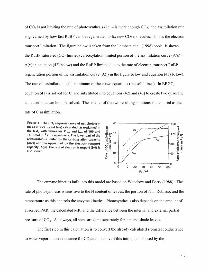
of CO2 is not limiting the rate of photosynthesis (i.e. – is there enough CO2), the assimilation rate
is governed by how fast RuBP can be regenerated to fix new CO2 molecules. This is the electron
transport limitation. The figure below is taken from the Lambers et al. (1998) book. It shows
the RuBP saturated (CO2 limited) carboxylation limited portion of the assimilation curve (A(c) –
A(v) in equation (42) below) and the RuBP limited due to the rate of electron transport RuBP
regeneration portion of the assimilation curve (A(j) in the figure below and equation (43) below).
The rate of assimilation is the minimum of these two equations (the solid lines). In BBGC,
equation (41) is solved for Ci and substituted into equations (42) and (43) to create two quadratic
equations that can both be solved. The smaller of the two resulting solutions is then used as the
rate of C assimilation.
The enzyme kinetics built into this model are based on Woodrow and Berry (1988). The
rate of photosynthesis is sensitive to the N content of leaves, the portion of N in Rubisco, and the
temperature as this controls the enzyme kinetics. Photosynthesis also depends on the amount of
absorbed PAR, the calculated MR, and the difference between the internal and external partial
pressure of CO2. As always, all steps are done separately for sun and shade leaves.
The first step in this calculation is to convert the already calculated stomatal conductance
to water vapor to a conductance for CO2 and to convert this into the units used by the

41
photosynthesis (PSYN) submodel (m/s to umol/m2/s/Pa). This conversion is seen below (Nobel
1991; Jones 1992):
(40) gmTc = ( )15.273*6.1*61+TdayRgE Tv
Where R is the universal gas constant, gTv is the leaf scale conductance to transpired water, tday
is the daytime temperature, and 1.6 is the ratio of the molecular weights of water vapor to CO2.
Once the leaf level conductance to CO2 is known, the main PSYN routine is begun. The
core logic of the PSYN routine consists of three main equations (Farquhar, Caemmerer et al.
1980):
(41) A(v or j) = gmTc * (Ca – Ci)
(42) Av = ( )leafday
oci
ic MR
KOKC
CV−
⎟⎟⎠
⎞⎜⎜⎝
⎛++
Γ−
2
*max
1*
(43) Aj = ( )
leafdayi
i MRC
CJ−
Γ+Γ−
*
*
*5.10*5.4*
Where Ca the atmospheric concentration of CO2 (Pa) and Ci is the intercellular
concentration of CO2 (Pa), Г* (Pa) is the CO2 compensation point in the absence of leaf MR, Kc
and Ko are the kinetic constants for rubisco carboxylation and oxygenation scaled by the
temperature using a Q10 relationship, O2 is the atmospheric concentration of O2 (Pa), MRleafday is
the daytime leaf maintenance respiration on a PLAI basis, and J is the maximum rate of electron
transport. Each of these variables will be discussed in more detail below.
Equation 40 represents the diffusion limitation of CO2 on assimilation. Equation 41
represents the carboxylation limitation on the rate of assimilation. Equation 42 represents the
electron transport rate of substrate regeneration limitation on assimilation. Thornton (1998)

42
explains that by solving equation 40 for Ci and then substituting this value back into equations 41
and 42, two quadratic equations are created that can be solved. The smaller of the two results
when solving both equations is then used as the actual assimilation rate.
There are several steps required to before the quadratic roots are ready to be calculated.
To begin, J must be calculated. J is a function of the maximum rate of carboxylation (Vcmax)
(Wullschleger 1993):
(44) Jmax = 2.1 * Vcmax
Vcmax is a function of the N per unit PLAI in the shade and sun leaves as well as the fraction of
leaf N in rubisco and the activation potential of rubisco as defined by the Woodrow and Berry
(1988):
(45) Vcmax = Nsun or shade leaves * fraction of leaf N in rubisco * 7.16 * ACT
The N content of sun and shade leaves is a function of the user defined ratio of C:N in leaves:
(46) Nsun of shade leaves = shadeorsunSLAleafNC :/1
The fraction of leaf N in rubisco is a user supplied parameter. 7.16 is the weight proportion of
rubisco relative to its N content (Kuehn and McFadden 1969; Kuehn and McFadden 1969;
Fasman 1976), and ACT is the activity of rubisco scaled by temperature and [O2] and [CO2].
The first step in calculating the enzyme kinetics of rubisco is to calculate the [O2] assuming it is
21% of the atmosphere by volume:
(47) O2 = 0.21 * atmospheric pressure (Pa)
Next, the rubisco activity can be calculated following its Michealis-Menten dynamics for
O2 and CO2 (the CO2 calculations vary depending on whether it is <= or > 15°C). All variables
with a 25 subscript are the constant values at 25°C that are being scaled based on temperature.
43
The different Q10 values relate to the different Q10 relationships with temperature for each of
these reactions.
(48) Ko = Ko25*⎟⎠⎞
⎜⎝⎛ −
1025
10
Tday
KoQ
(49) If tday > 15°C:
a. Kc = Kc25*⎟⎠⎞
⎜⎝⎛ −
1025
10
Tday
KcQ
b. ACT = ACT25*⎟⎠⎞
⎜⎝⎛ −
1025
10
Tday
ACTQ
(50) If tday <= 15°C:
a. Kc = c
c
K
Tday
Kc
QQK
10
1015
1025 8.1*⎟⎠⎞
⎜⎝⎛ −
b. ACT = ACT
Tday
ACT
QQACT
10
1015
1025 8.1*⎟⎠⎞
⎜⎝⎛ −
With ACT, Kc, and Ko calculated, Г* (Pa) (the CO2 compensation point in the absence of leaf
MR) and Vcmax can now be found. Г* is:
(51) Г* = 0.105 * Kc * oK
O2
All of these calculations are done for both sun and shade leaves and at the end of the day
the total assimilate is the sum of the sun and shade leaf assimilation. The assimilated C that is
calculated is actually a rate of C assimilation per second scaled by PLAI. This value must be
multiplied by the length of daylight and then multiplied by the sun or shade PLAI to find the
total C assimilated. This assimilate is converted from umol/m2/sec to kg/m2/day and then placed
into the Cpool for future allocation.

44
Given these assumptions and the model logic described above, users can have a high
degree of confidence in model runs with the major caveat that the user specified parameters need
to be appropriate for a given system. As stated before, when correctly parameterized to represent
a system, this model has been validated in many diverse systems across the globe. However, this
parameterization can at times feel quite arbitrary and there are a few parameters that really are
more “tuning dials” than real physiological system components (e.g. – soil depth). In this sense,
the model has made some conceptual abstractions to allow a user to represent a given system
with more certainty despite the underlying lack of clarity in the model representation of actual
physiological processes. This is always a tradeoff that any model is forced to make. In practice,
what this means is that BBGC can be used across many diverse systems with appropriate
calibration and in this sense, with a broad enough perspective, it is very valuable. However, to
explore specific physiological concepts that relate to specific plant communities, model
modifications may be required to more accurately represent the underlying mechanisms at work.
N Deposition and Fixation (within bgc.c):
The N deposition and N fixation are added to the soil mineral N pool.
H2O outflow (outflow.c):
Outflow occurs in two cases. First, for fast outflow, if the incoming precipitation causes
the soil water to exceed the saturated soil water capacity, outflow is the difference between the
soil water capacity and the remaining water over capacity. Second, for slow outflow, if the soil
water is above field capacity, then the outflow occurs at an exponentially decaying rate each day

45
with half of the water that is above field capacity draining. If the soil water is less than field
capacity, there is no outflow.
Decomposition (decomp.c):
The BBGC decomposition model is similar to the canopy evapotranspiration model logic
in that both use multiplicative scalars to adjust maximum rates. BBGC uses a compartment
system to represent the litter pools and the soil organic matter pools. The four litter pools are
broken out based on the dominant material found in them – labile carbon in the form of basic
sugars, starches, and proteins, unshielded cellulose, shielded cellulose with some lignin fraction,
and a lignin pool. A CWD pool accepts inputs from the stem and coarse root pools and
subsequently adds to the litter pools after it is broken into smaller pieces over time. Only fine
roots and leaves initially enter the litter pools. The fractions of leaf and fine root litter, as well as
the fractions of dead wood that are cellulose and lignin, are all user supplied and also are used to
calculated the shielded and unshielded fractions of the cellulose litter pool.

46
Taken from Thornton and Rosenbloom (2005). Changes reflect BiomeBGC v4.2 code.
SOM4.00010.0014
Lit4.0001
In this diagram, Lit4 is the shielded cellulosic litter. It is broken down at the same rate as the lignin pool (Lit3) and is transferred to the unshielded cellulosic litter pool (Lit2) as it decomposes. SOM4 is the recalcitrant soil organic matter pool (humus).
0.55
Figure 10: BiomeBGC litter and soil pools and fluxes
Upon decomposition, the litter pool fractions enter into the soil organic matter pools. The
maximum rate constants for decomposition and biomass loss through heterotrophic respiration
(HR) are all defined as constants in BBGC and were defined based on a literature review of C14
decomposition studies by Thornton (1998). Figure 10 is a detailed diagram of the decomposition
dynamics in BGC (Thornton and Rosenbloom 2005). The rates seen in this diagram are adjusted
based on the temperature (Lloyd and Taylor 1994) and the availability of water in the soil as seen
in figure 11 (Orchard and Cook 1983; Andren and Paustian 1987). There is no decomposition if
the temperature is below -10°C.
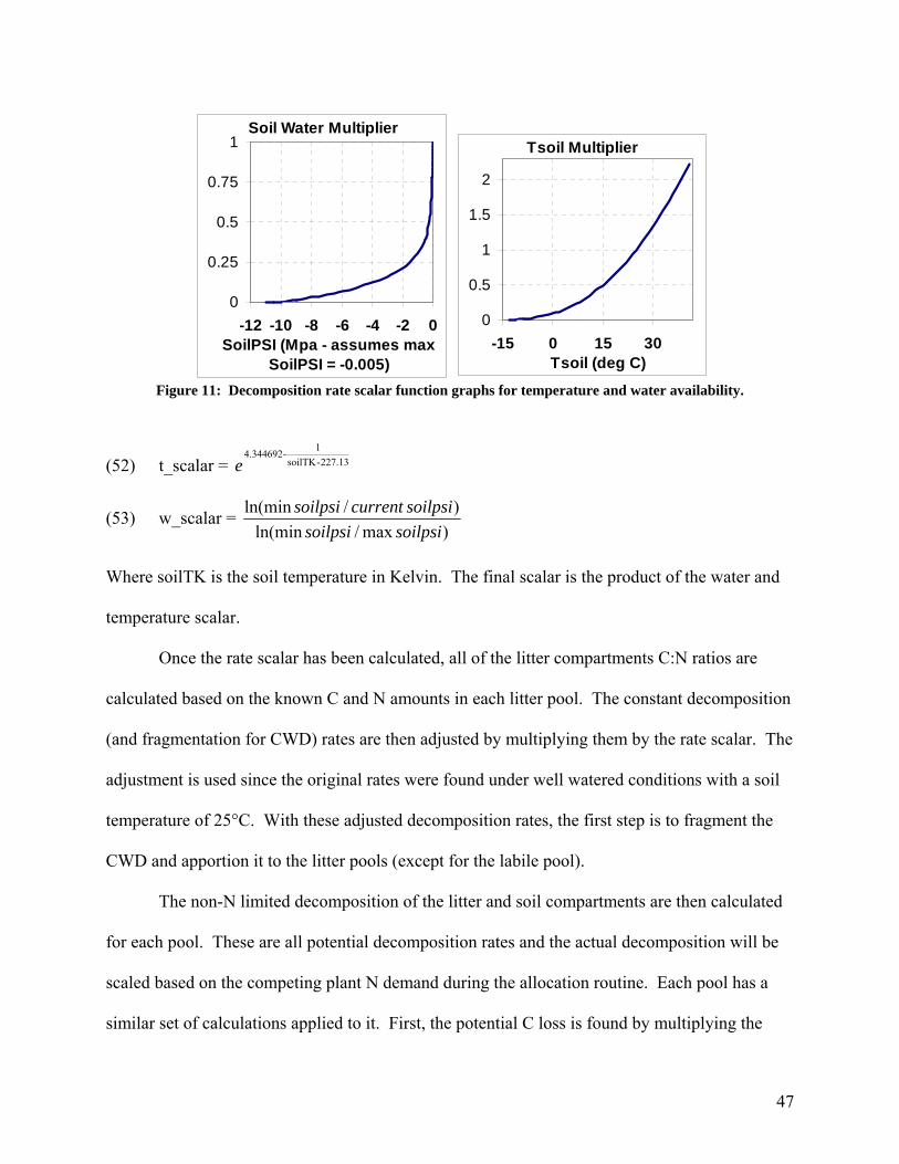
47
Soil Water Multiplier
0
0.25
0.5
0.75
1
-12 -10 -8 -6 -4 -2 0SoilPSI (Mpa - assumes max
SoilPSI = -0.005)
Tsoil Multiplier
0
0.5
1
1.5
2
-15 0 15 30Tsoil (deg C)
Figure 11: Decomposition rate scalar function graphs for temperature and water availability.
(52) t_scalar = 227.13-soilTK1-4.344692
e
(53) w_scalar = )max/ln(min
)/ln(minsoilpsisoilpsi
soilpsicurrentsoilpsi
Where soilTK is the soil temperature in Kelvin. The final scalar is the product of the water and
temperature scalar.
Once the rate scalar has been calculated, all of the litter compartments C:N ratios are
calculated based on the known C and N amounts in each litter pool. The constant decomposition
(and fragmentation for CWD) rates are then adjusted by multiplying them by the rate scalar. The
adjustment is used since the original rates were found under well watered conditions with a soil
temperature of 25°C. With these adjusted decomposition rates, the first step is to fragment the
CWD and apportion it to the litter pools (except for the labile pool).
The non-N limited decomposition of the litter and soil compartments are then calculated
for each pool. These are all potential decomposition rates and the actual decomposition will be
scaled based on the competing plant N demand during the allocation routine. Each pool has a
similar set of calculations applied to it. First, the potential C loss is found by multiplying the

48
adjusted decomposition rate by the amount of C in the litter pool. The ratio of the C:N ratio of
the given soil pool that accepts the decomposed matter to the C:N ratio of the litter pool that is
losing C is then found. The same step is performed for the soil to soil fluxes as well. The
potential N immobilization by microbial decomposition is then calculated from this data:
(54) potential N immobilization = potential C loss * poolacceptingNC
poolacceptingNCpooldonorNCHRfrac
::
:1 −−
As a last step, the sum of all of the potential N immobilization for the fluxes between the
pools is calculated. In some cases, given the C:N ratios of the pools, this may be a negative
number in which case this is considered potential N mineralization.
Allocation (daily_allocation.c):
With the amount of potential C assimilate known from the photosynthesis process, and
the amount of microbial N demand known from the decomposition process, it is now possible to
allocate C assimilate and account for N limitation. The BBGC allocation logic is built around
the concept that all new allocation is constrained by leaf C allocation (Waring and Pitman 1985;
Waring and Running 2007). There are four user defined allocation ratios for woody plants: 1)
new fine root C to new leaf C, 2) new stem C to new leaf C, 3) new live wood C to new total
wood C, and 4) new coarse root C to new stem C. There is also one user defined proportion that
defines how much of the assimilated C should be set aside for next year’s growth. These ratios
then are used to define how C is allocated throughout the plant.
The first step in the allocation is to find the C available to allocate. This is Gross Primary
Production (GPP) minus the MR of all live tissues. In some cases, the cpool variable that holds
the daily assimilated C and acts as a bank account for plant C demand can be negative. This

49
could occur, for example, if growing conditions prevented assimilation but MR was still
occurring. In these cases, a rate of repayment of this cpool deficit is calculated such that the
deficit is gone in one year and the available C for allocation is first allocated to alleviate the
deficit at this rate. Any leftover C can then be allocated to plant growth.
The next step is to calculate the amount of C needed per unit of leaf C growth in all of the
other pools based on the allocation fractions described above as well as the amount of C needed
for growth respiration based on this allocation. BBGC assumes a constant rate of GR for all
tissue growth = 30% of the total C used for new tissue. The C allometry calculation is followed
by calculating the associated N needed to grow the plant based on this C allometry and the
respective C:N ratios of the different plant pools.
(55) C needed / unit leaf C = (1 + GR%) * ⎟⎟⎠
⎞⎜⎜⎝
⎛⎟⎠⎞
⎜⎝⎛ +++
stemCcrootC
leafCstemC
leafCfrC 1*1
(56) N needed / unit leaf N =
NDeadWoodC:
stemC
crootC*
NwoodC
NLwoodC*
leafC
stemC
NLiveWoodC:
stemC
crootC*
NwoodC
NLwoodC*
leafC
stemC
frC:N
leafC
frC
LeafC:N
⎟⎠⎞
⎜⎝⎛
⎟⎠⎞
⎜⎝⎛
⎟⎠⎞
⎜⎝⎛
+−
+
+
+−
1111
Where NLwood is new live wood and Nwood is total new wood both live and dead and croot is
coarse root.
Dividing equation 54 by equation 55 gives the C:N ratio of newly allocated tissue.
Multiplying this by the C available for allocation tells us the plant N demand given the potential
C to allocate. The total N demand in the system is also know since the potential microbial N
demand from the decomposition function is now known. If the total system N demand is less
than the available soil mineral N (SMN) pool actual allocation is equal to potential allocation and
actual decomposition is also potential decomposition. If the available retranslocated N can

50
satisfy the plant N demand, the plant N demand quantity is shifted from the retranslocation pool
to the npool to be allocated at the end of the daily loop. If not, the total daily N retranslocated is
applied to plant N demand and the additional N needed is removed from the SMN pool. Half of
any excess N is assumed mineralized each day and is added to a bulk denitrification flux
(volatilization) to be deducted from the SMN pool.
If there is less SMN than total demand, the potential N immobilization flux (the potential
microbial decomposition) is scaled based on the ratio of the potential immobilization to the total
system N demand. The fraction of potential N immobilization (FPI) is then:
(57) FPI = tionimmobilizaNpotential
demandNtotaltionimmobilizaNpotentialSMN *
=tionimmobilizaNpotential
tionimmobilizaNactual
Once the microbial N demand is partially satisfied in this way, the plant N demand is addressed
by first looking at the available retranslocated N pool. If there is enough retranslocated N and
SMN available, plant C allocation will not be limited by N and will proceed at its potential rate.
If there is not enough retranslocated N to meet the plant N demand, the C assimilate available for
allocation is proportionally reduced (for both shade and sun leaves – Wang et al. noted this and
postulated that this should be accounted for by greater respiration costs instead of scaling the
amount of assimilated C (Wang, Ichii et al. 2009)). The actual C allocated to new growth is then
the actual N available for plants * the N:C allometry ratios defined in equations 54 and 55. The
excess C is removed from the assimilated C for sun and shade leaves in proportion to their size
relative to total GPP and this serves as another limit on plant photosynthetic capacity.
With the actual allocation amounts now known, BBGC moves the assimilated C and the
associated N into the different tissue pools and storage pools for next year’s growth. This
function also then scales each potential decomposition flux based on the FPI calculated above.

51
One other point to note is that during spin-up runs, BBGC adds additional N to the system if N is
limiting to speed the systems’ attainment of its steady-state result.
Growth Respiration (growth_resp.c):
The GR function simply allocates the C to the GR pools and the storage GR pools for
next year’s growth. These quantities were already calculated in the daily allocation routine.
Update C, N, and H2O state (state_update.c):
After the functions above have been completed, BBGC moves the fluxes identified to and
from the C, N, and H2O state pools. All of the functions above do not modify the actual states
but rather updates flux variables that are then modified in the state_update routine. On the last
day of the year, the storage C and N pools are moved to become transfer pools that can then be
used for the next year’s growth.
N Leaching (nleaching.c):
N leaching only occurs if there was water outflow. If there was outflow, then 10% of the
SMN is removed and considered leached.
Mortality (mortality.c):
The daily mortality fraction is user defined in the epc file and is applied to all plant pools
both live and dead as well as the transfer and storage pools. This function partitions the
mortality into the appropriate CWD and litter pools. The mortality function also applies any user
specified fire mortality to plant C and N pools moving the specified daily proportion from the

52
pools into a fire sink pool that represents the loss of C and N to the atmosphere. The fire routine
also assumes there will be some recruitment of CWD and therefore only applies 30% of the fire
mortality loss to the CWD pool.
Mass Balance Check (check_balance.c):
Once all of the state variables have been updated by both the state update routine and the
mortality function, the check balance function is called to insure the Principle of the
Conservation of Mass. Table 1 shows all of the sources, outflows/removals, and storage pools
for C, N, and H2O that the model tracks and balances by testing whether the balance is <=
0.00000001. The daily balance is defined as:
(58) Balance = in – out – stores
The only balance that is not checked (but probably should be) is the radiation energy balance.
Table 1: BiomeBGC inputs, outputs, and storage for mass balance check. In Out Storage
H2O (see figure 3) Precipitation
Outflow Soil evaporation Snow sublimation Canopy evaporation Leaf transpiration
Soil water Snow water Canopy water
C (S and T refer to
Storage and Transfer
Pools) (see figure 4)
Sun leaf psyn Shade leaf psyn
Leaf MR and GR Fine root MR and GR Live stem MR and GR Live coarse root MR and GR Dead stem GR Dead coarse root GR Labile litter (litter 1) HR Cellulose litter (litter 2) HR Lignin litter (litter 4) HR Fast Soil (SOM1) HR Medium Soil (SOM2) HR Slow Soil (SOM3) HR Recalcitrant Soil (SOM4) HR Fire
Leaf C and S and T Fine root and S and T Live stem and S and T Dead stem and S and T Live Coarse Root and S and T Dead Coarse Root and S and T CWD Litter Pools 1-4 SOM Pools 1-4 Cpool

53
N (S and T refer to
Storage and Transfer
Pools) (see figure 4)
N fixation N Deposition
N leaching N volatilization (denitrification) Fire loss N
Leaf N and S and T Fine root and S and T Live stem and S and T Dead stem and S and T Live coarse root and S and T Dead coarse root and S and T CWD Litter pools 1-4 SOM pools 1-4 Soil Mineral N Retranslocated N Pool Npool
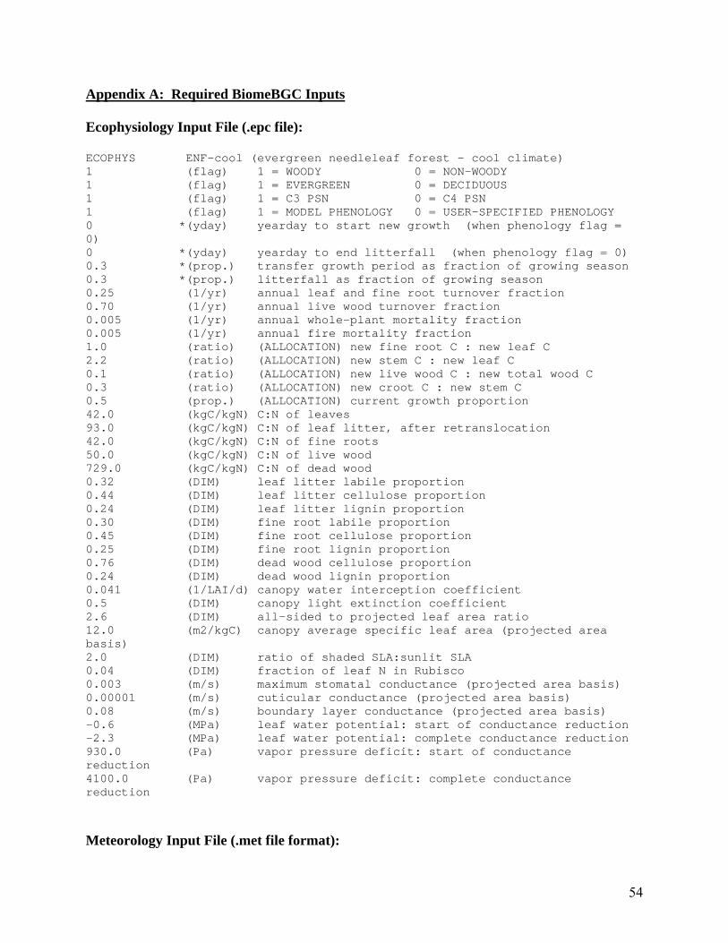
54
Appendix A: Required BiomeBGC Inputs
Ecophysiology Input File (.epc file):
ECOPHYS ENF-cool (evergreen needleleaf forest - cool climate) 1 (flag) 1 = WOODY 0 = NON-WOODY 1 (flag) 1 = EVERGREEN 0 = DECIDUOUS 1 (flag) 1 = C3 PSN 0 = C4 PSN 1 (flag) 1 = MODEL PHENOLOGY 0 = USER-SPECIFIED PHENOLOGY 0 *(yday) yearday to start new growth (when phenology flag = 0) 0 *(yday) yearday to end litterfall (when phenology flag = 0) 0.3 *(prop.) transfer growth period as fraction of growing season 0.3 *(prop.) litterfall as fraction of growing season 0.25 (1/yr) annual leaf and fine root turnover fraction 0.70 (1/yr) annual live wood turnover fraction 0.005 (1/yr) annual whole-plant mortality fraction 0.005 (1/yr) annual fire mortality fraction 1.0 (ratio) (ALLOCATION) new fine root C : new leaf C 2.2 (ratio) (ALLOCATION) new stem C : new leaf C 0.1 (ratio) (ALLOCATION) new live wood C : new total wood C 0.3 (ratio) (ALLOCATION) new croot C : new stem C 0.5 (prop.) (ALLOCATION) current growth proportion 42.0 (kgC/kgN) C:N of leaves 93.0 (kgC/kgN) C:N of leaf litter, after retranslocation 42.0 (kgC/kgN) C:N of fine roots 50.0 (kgC/kgN) C:N of live wood 729.0 (kgC/kgN) C:N of dead wood 0.32 (DIM) leaf litter labile proportion 0.44 (DIM) leaf litter cellulose proportion 0.24 (DIM) leaf litter lignin proportion 0.30 (DIM) fine root labile proportion 0.45 (DIM) fine root cellulose proportion 0.25 (DIM) fine root lignin proportion 0.76 (DIM) dead wood cellulose proportion 0.24 (DIM) dead wood lignin proportion 0.041 (1/LAI/d) canopy water interception coefficient 0.5 (DIM) canopy light extinction coefficient 2.6 (DIM) all-sided to projected leaf area ratio 12.0 (m2/kgC) canopy average specific leaf area (projected area basis) 2.0 (DIM) ratio of shaded SLA:sunlit SLA 0.04 (DIM) fraction of leaf N in Rubisco 0.003 (m/s) maximum stomatal conductance (projected area basis) 0.00001 (m/s) cuticular conductance (projected area basis) 0.08 (m/s) boundary layer conductance (projected area basis) -0.6 (MPa) leaf water potential: start of conductance reduction -2.3 (MPa) leaf water potential: complete conductance reduction 930.0 (Pa) vapor pressure deficit: start of conductance reduction 4100.0 (Pa) vapor pressure deficit: complete conductance reduction
Meteorology Input File (.met file format):

55
Missoula, 1950-1993 : Sample input for MTCLIM v4.1 MTCLIM v4.1 OUTPUT FILE : Tue Aug 25 10:15:00 1998 year yday Tmax Tmin Tday prcp VPD srad daylen (deg C) (deg C) (deg C) (cm) (Pa) (W m-2) (s) 1950 1 -3.90 -13.90 -6.65 0.10 158.19 123.31 30229 1950 2 -7.80 -21.70 -11.62 0.00 136.27 183.78 30284 1950 3 -16.10 -23.30 -18.08 0.00 53.36 140.67 30344
Physical Site Input File (.ini file):
Biome-BGC v4.1.2 example : (normal simulation, Missoula, evergreen needleleaf) MET_INPUT (keyword) start of meteorology file control block metdata/miss5093.mtc41 meteorology input filename 4 (int) header lines in met file RESTART (keyword) start of restart control block 0 (flag) 1 = read restart file 0 = don't read restart file 0 (flag) 1 = write restart file 0 = don't write restart file 1 (flag) 1 = use restart metyear 0 = reset metyear restart/enf_test1.endpoint input restart filename restart/enf_test1.endpoint output restart filename TIME_DEFINE (keyword - do not remove) 44 (int) number of meteorological data years 44 (int) number of simulation years 1950 (int) first simulation year 0 (flag) 1 = spinup simulation 0 = normal simulation 6000 (int) maximum number of spinup years (if spinup simulation) CLIM_CHANGE (keyword - do not remove) 0.0 (deg C) offset for Tmax 0.0 (deg C) offset for Tmin 1.0 (DIM) multiplier for Prcp 1.0 (DIM) multiplier for VPD 1.0 (DIM) multiplier for shortwave radiation CO2_CONTROL (keyword - do not remove) 0 (flag) 0=constant 1=vary with file 2=constant, file for Ndep 294.842 (ppm) constant atmospheric CO2 concentration xxxxxxxxxxx (file) annual variable CO2 filename SITE (keyword) start of site physical constants block 1.0 (m) effective soil depth (corrected for rock fraction) 30.0 (%) sand percentage by volume in rock-free soil 50.0 (%) silt percentage by volume in rock-free soil 20.0 (%) clay percentage by volume in rock-free soil 977.0 (m) site elevation 46.8 (degrees) site latitude (- for S.Hem.) 0.2 (DIM) site shortwave albedo 0.0001 (kgN/m2/yr) wet+dry atmospheric deposition of N 0.0004 (kgN/m2/yr) symbiotic+asymbiotic fixation of N

56
RAMP_NDEP (keyword - do not remove) 0 (flag) do a ramped N-deposition run? 0=no, 1=yes 2099 (int) reference year for industrial N deposition 0.0001 (kgN/m2/yr) industrial N deposition value EPC_FILE (keyword - do not remove) epc/enf.epc (file) evergreen needleleaf forest ecophysiological constants W_STATE (keyword) start of water state variable initialization block 0.0 (kg/m2) water stored in snowpack 0.5 (DIM) initial soil water as a proportion of saturation C_STATE (keyword) start of carbon state variable initialization block 0.001 (kgC/m2) first-year maximum leaf carbon 0.0 (kgC/m2) first-year maximum stem carbon 0.0 (kgC/m2) coarse woody debris carbon 0.0 (kgC/m2) litter carbon, labile pool 0.0 (kgC/m2) litter carbon, unshielded cellulose pool 0.0 (kgC/m2) litter carbon, shielded cellulose pool 0.0 (kgC/m2) litter carbon, lignin pool 0.0 (kgC/m2) soil carbon, fast microbial recycling pool 0.0 (kgC/m2) soil carbon, medium microbial recycling pool 0.0 (kgC/m2) soil carbon, slow microbial recycling pool 0.0 (kgC/m2) soil carbon, recalcitrant SOM (slowest) N_STATE (keyword) start of nitrogen state variable initialization block 0.0 (kgN/m2) litter nitrogen, labile pool 0.0 (kgN/m2) soil nitrogen, mineral pool OUTPUT_CONTROL (keyword - do not remove) outputs/oth (text) prefix for output files 1 (flag) 1 = write daily output 0 = no daily output 1 (flag) 1 = monthly avg of daily variables 0 = no monthly avg 1 (flag) 1 = annual avg of daily variables 0 = no annual avg 1 (flag) 1 = write annual output 0 = no annual output 1 (flag) for on-screen progress indicator DAILY_OUTPUT (keyword) 23 (int) number of daily variables to output 20 0 ws.soilw 21 1 ws.snoww 38 2 wf.canopyw_evap 40 3 wf.snoww_subl 42 4 wf.soilw_evap 43 5 wf.soilw_trans 44 6 wf.soilw_outflow 70 7 cs.cwdc 509 8 epv.proj_lai 528 9 epv.daily_net_nmin 620 10 summary.daily_npp 621 11 summary.daily_nep 622 12 summary.daily_nee 623 13 summary.daily_gpp 624 14 summary.daily_mr 625 15 summary.daily_gr 626 16 summary.daily_hr
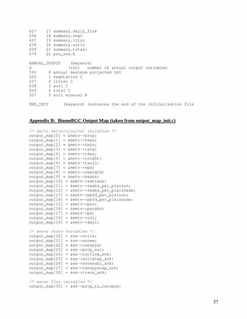
57
627 17 summary.daily_fire 636 18 summary.vegc 637 19 summary.litrc 638 20 summary.soilc 639 21 summary.totalc 579 22 psn_sun.A ANNUAL_OUTPUT (keyword) 6 (int) number of annual output variables 545 0 annual maximum projected LAI 636 1 vegetation C 637 2 litter C 638 3 soil C 639 4 total C 307 5 soil mineral N END_INIT (keyword) indicates the end of the initialization file
Appendix B: BiomeBGC Output Map (taken from output_map_init.c)
/* daily meteorological variables */ output_map[0] = &metv->prcp; output_map[1] = &metv->tmax; output_map[2] = &metv->tmin; output_map[3] = &metv->tavg; output_map[4] = &metv->tday; output_map[5] = &metv->tnight; output_map[6] = &metv->tsoil; output_map[7] = &metv->vpd; output_map[8] = &metv->swavgfd; output_map[9] = &metv->swabs; output_map[10] = &metv->swtrans; output_map[11] = &metv->swabs_per_plaisun; output_map[12] = &metv->swabs_per_plaishade; output_map[13] = &metv->ppfd_per_plaisun; output_map[14] = &metv->ppfd_per_plaishade; output_map[15] = &metv->par; output_map[16] = &metv->parabs; output_map[17] = &metv->pa; output_map[18] = &metv->co2; output_map[19] = &metv->dayl; /* water state variables */ output_map[20] = &ws->soilw; output_map[21] = &ws->snoww; output_map[22] = &ws->canopyw; output_map[23] = &ws->prcp_src; output_map[24] = &ws->outflow_snk; output_map[25] = &ws->soilevap_snk; output_map[26] = &ws->snowsubl_snk; output_map[27] = &ws->canopyevap_snk; output_map[28] = &ws->trans_snk; /* water flux variables */ output_map[35] = &wf->prcp_to_canopyw;

58
output_map[36] = &wf->prcp_to_soilw; output_map[37] = &wf->prcp_to_snoww; output_map[38] = &wf->canopyw_evap; output_map[39] = &wf->canopyw_to_soilw; output_map[40] = &wf->snoww_subl; output_map[41] = &wf->snoww_to_soilw; output_map[42] = &wf->soilw_evap; output_map[43] = &wf->soilw_trans; output_map[44] = &wf->soilw_outflow; /* carbon state variables */ output_map[50] = &cs->leafc; output_map[51] = &cs->leafc_storage; output_map[52] = &cs->leafc_transfer; output_map[53] = &cs->frootc; output_map[54] = &cs->frootc_storage; output_map[55] = &cs->frootc_transfer; output_map[56] = &cs->livestemc; output_map[57] = &cs->livestemc_storage; output_map[58] = &cs->livestemc_transfer; output_map[59] = &cs->deadstemc; output_map[60] = &cs->deadstemc_storage; output_map[61] = &cs->deadstemc_transfer; output_map[62] = &cs->livecrootc; output_map[63] = &cs->livecrootc_storage; output_map[64] = &cs->livecrootc_transfer; output_map[65] = &cs->deadcrootc; output_map[66] = &cs->deadcrootc_storage; output_map[67] = &cs->deadcrootc_transfer; output_map[68] = &cs->gresp_storage; output_map[69] = &cs->gresp_transfer; output_map[70] = &cs->cwdc; output_map[71] = &cs->litr1c; output_map[72] = &cs->litr2c; output_map[73] = &cs->litr3c; output_map[74] = &cs->litr4c; output_map[75] = &cs->soil1c; output_map[76] = &cs->soil2c; output_map[77] = &cs->soil3c; output_map[78] = &cs->soil4c; output_map[79] = &cs->cpool; output_map[80] = &cs->psnsun_src; output_map[81] = &cs->psnshade_src; output_map[82] = &cs->leaf_mr_snk; output_map[83] = &cs->leaf_gr_snk; output_map[84] = &cs->froot_mr_snk; output_map[85] = &cs->froot_gr_snk; output_map[86] = &cs->livestem_mr_snk; output_map[87] = &cs->livestem_gr_snk; output_map[88] = &cs->deadstem_gr_snk; output_map[89] = &cs->livecroot_mr_snk; output_map[90] = &cs->livecroot_gr_snk; output_map[91] = &cs->deadcroot_gr_snk; output_map[92] = &cs->litr1_hr_snk; output_map[93] = &cs->litr2_hr_snk; output_map[94] = &cs->litr4_hr_snk; output_map[95] = &cs->soil1_hr_snk;

59
output_map[96] = &cs->soil2_hr_snk; output_map[97] = &cs->soil3_hr_snk; output_map[98] = &cs->soil4_hr_snk; output_map[99] = &cs->fire_snk; /* carbon flux variables */ output_map[120] = &cf->m_leafc_to_litr1c; output_map[121] = &cf->m_leafc_to_litr2c; output_map[122] = &cf->m_leafc_to_litr3c; output_map[123] = &cf->m_leafc_to_litr4c; output_map[124] = &cf->m_frootc_to_litr1c; output_map[125] = &cf->m_frootc_to_litr2c; output_map[126] = &cf->m_frootc_to_litr3c; output_map[127] = &cf->m_frootc_to_litr4c; output_map[128] = &cf->m_leafc_storage_to_litr1c; output_map[129] = &cf->m_frootc_storage_to_litr1c; output_map[130] = &cf->m_livestemc_storage_to_litr1c; output_map[131] = &cf->m_deadstemc_storage_to_litr1c; output_map[132] = &cf->m_livecrootc_storage_to_litr1c; output_map[133] = &cf->m_deadcrootc_storage_to_litr1c; output_map[134] = &cf->m_leafc_transfer_to_litr1c; output_map[135] = &cf->m_frootc_transfer_to_litr1c; output_map[136] = &cf->m_livestemc_transfer_to_litr1c; output_map[137] = &cf->m_deadstemc_transfer_to_litr1c; output_map[138] = &cf->m_livecrootc_transfer_to_litr1c; output_map[139] = &cf->m_deadcrootc_transfer_to_litr1c; output_map[140] = &cf->m_livestemc_to_cwdc; output_map[141] = &cf->m_deadstemc_to_cwdc; output_map[142] = &cf->m_livecrootc_to_cwdc; output_map[143] = &cf->m_deadcrootc_to_cwdc; output_map[144] = &cf->m_gresp_storage_to_litr1c; output_map[145] = &cf->m_gresp_transfer_to_litr1c; output_map[146] = &cf->m_leafc_to_fire; output_map[147] = &cf->m_frootc_to_fire; output_map[148] = &cf->m_leafc_storage_to_fire; output_map[149] = &cf->m_frootc_storage_to_fire; output_map[150] = &cf->m_livestemc_storage_to_fire; output_map[151] = &cf->m_deadstemc_storage_to_fire; output_map[152] = &cf->m_livecrootc_storage_to_fire; output_map[153] = &cf->m_deadcrootc_storage_to_fire; output_map[154] = &cf->m_leafc_transfer_to_fire; output_map[155] = &cf->m_frootc_transfer_to_fire; output_map[156] = &cf->m_livestemc_transfer_to_fire; output_map[157] = &cf->m_deadstemc_transfer_to_fire; output_map[158] = &cf->m_livecrootc_transfer_to_fire; output_map[159] = &cf->m_deadcrootc_transfer_to_fire; output_map[160] = &cf->m_livestemc_to_fire; output_map[161] = &cf->m_deadstemc_to_fire; output_map[162] = &cf->m_livecrootc_to_fire; output_map[163] = &cf->m_deadcrootc_to_fire; output_map[164] = &cf->m_gresp_storage_to_fire; output_map[165] = &cf->m_gresp_transfer_to_fire; output_map[166] = &cf->m_litr1c_to_fire; output_map[167] = &cf->m_litr2c_to_fire; output_map[168] = &cf->m_litr3c_to_fire; output_map[169] = &cf->m_litr4c_to_fire; output_map[170] = &cf->m_cwdc_to_fire;

60
output_map[171] = &cf->leafc_transfer_to_leafc; output_map[172] = &cf->frootc_transfer_to_frootc; output_map[173] = &cf->livestemc_transfer_to_livestemc; output_map[174] = &cf->deadstemc_transfer_to_deadstemc; output_map[175] = &cf->livecrootc_transfer_to_livecrootc; output_map[176] = &cf->deadcrootc_transfer_to_deadcrootc; output_map[177] = &cf->leafc_to_litr1c; output_map[178] = &cf->leafc_to_litr2c; output_map[179] = &cf->leafc_to_litr3c; output_map[180] = &cf->leafc_to_litr4c; output_map[181] = &cf->frootc_to_litr1c; output_map[182] = &cf->frootc_to_litr2c; output_map[183] = &cf->frootc_to_litr3c; output_map[184] = &cf->frootc_to_litr4c; output_map[185] = &cf->leaf_day_mr; output_map[186] = &cf->leaf_night_mr; output_map[187] = &cf->froot_mr; output_map[188] = &cf->livestem_mr; output_map[189] = &cf->livecroot_mr; output_map[190] = &cf->psnsun_to_cpool; output_map[191] = &cf->psnshade_to_cpool; output_map[192] = &cf->cwdc_to_litr2c; output_map[193] = &cf->cwdc_to_litr3c; output_map[194] = &cf->cwdc_to_litr4c; output_map[195] = &cf->litr1_hr; output_map[196] = &cf->litr1c_to_soil1c; output_map[197] = &cf->litr2_hr; output_map[198] = &cf->litr2c_to_soil2c; output_map[199] = &cf->litr3c_to_litr2c; output_map[200] = &cf->litr4_hr; output_map[201] = &cf->litr4c_to_soil3c; output_map[202] = &cf->soil1_hr; output_map[203] = &cf->soil1c_to_soil2c; output_map[204] = &cf->soil2_hr; output_map[205] = &cf->soil2c_to_soil3c; output_map[206] = &cf->soil3_hr; output_map[207] = &cf->soil3c_to_soil4c; output_map[208] = &cf->soil4_hr; output_map[209] = &cf->cpool_to_leafc; output_map[210] = &cf->cpool_to_leafc_storage; output_map[211] = &cf->cpool_to_frootc; output_map[212] = &cf->cpool_to_frootc_storage; output_map[213] = &cf->cpool_to_livestemc; output_map[214] = &cf->cpool_to_livestemc_storage; output_map[215] = &cf->cpool_to_deadstemc; output_map[216] = &cf->cpool_to_deadstemc_storage; output_map[217] = &cf->cpool_to_livecrootc; output_map[218] = &cf->cpool_to_livecrootc_storage; output_map[219] = &cf->cpool_to_deadcrootc; output_map[220] = &cf->cpool_to_deadcrootc_storage; output_map[221] = &cf->cpool_to_gresp_storage; output_map[222] = &cf->cpool_leaf_gr; output_map[223] = &cf->transfer_leaf_gr; output_map[224] = &cf->cpool_froot_gr; output_map[225] = &cf->transfer_froot_gr; output_map[226] = &cf->cpool_livestem_gr; output_map[227] = &cf->transfer_livestem_gr;
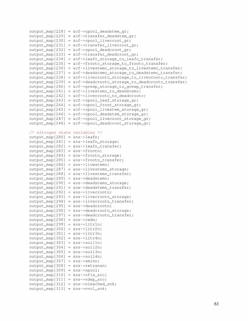
61
output_map[228] = &cf->cpool_deadstem_gr; output_map[229] = &cf->transfer_deadstem_gr; output_map[230] = &cf->cpool_livecroot_gr; output_map[231] = &cf->transfer_livecroot_gr; output_map[232] = &cf->cpool_deadcroot_gr; output_map[233] = &cf->transfer_deadcroot_gr; output_map[234] = &cf->leafc_storage_to_leafc_transfer; output_map[235] = &cf->frootc_storage_to_frootc_transfer; output_map[236] = &cf->livestemc_storage_to_livestemc_transfer; output_map[237] = &cf->deadstemc_storage_to_deadstemc_transfer; output_map[238] = &cf->livecrootc_storage_to_livecrootc_transfer; output_map[239] = &cf->deadcrootc_storage_to_deadcrootc_transfer; output_map[240] = &cf->gresp_storage_to_gresp_transfer; output_map[241] = &cf->livestemc_to_deadstemc; output_map[242] = &cf->livecrootc_to_deadcrootc; output_map[243] = &cf->cpool_leaf_storage_gr; output_map[244] = &cf->cpool_froot_storage_gr; output_map[245] = &cf->cpool_livestem_storage_gr; output_map[246] = &cf->cpool_deadstem_storage_gr; output_map[247] = &cf->cpool_livecroot_storage_gr; output_map[248] = &cf->cpool_deadcroot_storage_gr; /* nitrogen state variables */ output_map[280] = &ns->leafn; output_map[281] = &ns->leafn_storage; output_map[282] = &ns->leafn_transfer; output_map[283] = &ns->frootn; output_map[284] = &ns->frootn_storage; output_map[285] = &ns->frootn_transfer; output_map[286] = &ns->livestemn; output_map[287] = &ns->livestemn_storage; output_map[288] = &ns->livestemn_transfer; output_map[289] = &ns->deadstemn; output_map[290] = &ns->deadstemn_storage; output_map[291] = &ns->deadstemn_transfer; output_map[292] = &ns->livecrootn; output_map[293] = &ns->livecrootn_storage; output_map[294] = &ns->livecrootn_transfer; output_map[295] = &ns->deadcrootn; output_map[296] = &ns->deadcrootn_storage; output_map[297] = &ns->deadcrootn_transfer; output_map[298] = &ns->cwdn; output_map[299] = &ns->litr1n; output_map[300] = &ns->litr2n; output_map[301] = &ns->litr3n; output_map[302] = &ns->litr4n; output_map[303] = &ns->soil1n; output_map[304] = &ns->soil2n; output_map[305] = &ns->soil3n; output_map[306] = &ns->soil4n; output_map[307] = &ns->sminn; output_map[308] = &ns->retransn; output_map[309] = &ns->npool; output_map[310] = &ns->nfix_src; output_map[311] = &ns->ndep_src; output_map[312] = &ns->nleached_snk; output_map[313] = &ns->nvol_snk;

62
output_map[314] = &ns->fire_snk; /* nitrogen flux variables */ output_map[340] = &nf->m_leafn_to_litr1n; output_map[341] = &nf->m_leafn_to_litr2n; output_map[342] = &nf->m_leafn_to_litr3n; output_map[343] = &nf->m_leafn_to_litr4n; output_map[344] = &nf->m_frootn_to_litr1n; output_map[345] = &nf->m_frootn_to_litr2n; output_map[346] = &nf->m_frootn_to_litr3n; output_map[347] = &nf->m_frootn_to_litr4n; output_map[348] = &nf->m_leafn_storage_to_litr1n; output_map[349] = &nf->m_frootn_storage_to_litr1n; output_map[350] = &nf->m_livestemn_storage_to_litr1n; output_map[351] = &nf->m_deadstemn_storage_to_litr1n; output_map[352] = &nf->m_livecrootn_storage_to_litr1n; output_map[353] = &nf->m_deadcrootn_storage_to_litr1n; output_map[354] = &nf->m_leafn_transfer_to_litr1n; output_map[355] = &nf->m_frootn_transfer_to_litr1n; output_map[356] = &nf->m_livestemn_transfer_to_litr1n; output_map[357] = &nf->m_deadstemn_transfer_to_litr1n; output_map[358] = &nf->m_livecrootn_transfer_to_litr1n; output_map[359] = &nf->m_deadcrootn_transfer_to_litr1n; output_map[360] = &nf->m_livestemn_to_litr1n; output_map[361] = &nf->m_livestemn_to_cwdn; output_map[362] = &nf->m_deadstemn_to_cwdn; output_map[363] = &nf->m_livecrootn_to_litr1n; output_map[364] = &nf->m_livecrootn_to_cwdn; output_map[365] = &nf->m_deadcrootn_to_cwdn; output_map[366] = &nf->m_retransn_to_litr1n; output_map[367] = &nf->m_leafn_to_fire; output_map[368] = &nf->m_frootn_to_fire; output_map[369] = &nf->m_leafn_storage_to_fire; output_map[370] = &nf->m_frootn_storage_to_fire; output_map[371] = &nf->m_livestemn_storage_to_fire; output_map[372] = &nf->m_deadstemn_storage_to_fire; output_map[373] = &nf->m_livecrootn_storage_to_fire; output_map[374] = &nf->m_deadcrootn_storage_to_fire; output_map[375] = &nf->m_leafn_transfer_to_fire; output_map[376] = &nf->m_frootn_transfer_to_fire; output_map[377] = &nf->m_livestemn_transfer_to_fire; output_map[378] = &nf->m_deadstemn_transfer_to_fire; output_map[379] = &nf->m_livecrootn_transfer_to_fire; output_map[380] = &nf->m_deadcrootn_transfer_to_fire; output_map[381] = &nf->m_livestemn_to_fire; output_map[382] = &nf->m_deadstemn_to_fire; output_map[383] = &nf->m_livecrootn_to_fire; output_map[384] = &nf->m_deadcrootn_to_fire; output_map[385] = &nf->m_retransn_to_fire; output_map[386] = &nf->m_litr1n_to_fire; output_map[387] = &nf->m_litr2n_to_fire; output_map[388] = &nf->m_litr3n_to_fire; output_map[389] = &nf->m_litr4n_to_fire; output_map[390] = &nf->m_cwdn_to_fire; output_map[391] = &nf->leafn_transfer_to_leafn; output_map[392] = &nf->frootn_transfer_to_frootn; output_map[393] = &nf->livestemn_transfer_to_livestemn;

63
output_map[394] = &nf->deadstemn_transfer_to_deadstemn; output_map[395] = &nf->livecrootn_transfer_to_livecrootn; output_map[396] = &nf->deadcrootn_transfer_to_deadcrootn; output_map[397] = &nf->leafn_to_litr1n; output_map[398] = &nf->leafn_to_litr2n; output_map[399] = &nf->leafn_to_litr3n; output_map[400] = &nf->leafn_to_litr4n; output_map[401] = &nf->leafn_to_retransn; output_map[402] = &nf->frootn_to_litr1n; output_map[403] = &nf->frootn_to_litr2n; output_map[404] = &nf->frootn_to_litr3n; output_map[405] = &nf->frootn_to_litr4n; output_map[406] = &nf->ndep_to_sminn; output_map[407] = &nf->nfix_to_sminn; output_map[408] = &nf->cwdn_to_litr2n; output_map[409] = &nf->cwdn_to_litr3n; output_map[410] = &nf->cwdn_to_litr4n; output_map[411] = &nf->litr1n_to_soil1n; output_map[412] = &nf->sminn_to_soil1n_l1; output_map[413] = &nf->litr2n_to_soil2n; output_map[414] = &nf->sminn_to_soil2n_l2; output_map[415] = &nf->litr3n_to_litr2n; output_map[416] = &nf->litr4n_to_soil3n; output_map[417] = &nf->sminn_to_soil3n_l4; output_map[418] = &nf->soil1n_to_soil2n; output_map[419] = &nf->sminn_to_soil2n_s1; output_map[420] = &nf->soil2n_to_soil3n; output_map[421] = &nf->sminn_to_soil3n_s2; output_map[422] = &nf->soil3n_to_soil4n; output_map[423] = &nf->sminn_to_soil4n_s3; output_map[424] = &nf->soil4n_to_sminn; output_map[425] = &nf->sminn_to_nvol_l1s1; output_map[426] = &nf->sminn_to_nvol_l2s2; output_map[427] = &nf->sminn_to_nvol_l4s3; output_map[428] = &nf->sminn_to_nvol_s1s2; output_map[429] = &nf->sminn_to_nvol_s2s3; output_map[430] = &nf->sminn_to_nvol_s3s4; output_map[431] = &nf->sminn_to_nvol_s4; output_map[432] = &nf->sminn_leached; output_map[433] = &nf->retransn_to_npool; output_map[434] = &nf->sminn_to_npool; output_map[435] = &nf->npool_to_leafn; output_map[436] = &nf->npool_to_leafn_storage; output_map[437] = &nf->npool_to_frootn; output_map[438] = &nf->npool_to_frootn_storage; output_map[439] = &nf->npool_to_livestemn; output_map[440] = &nf->npool_to_livestemn_storage; output_map[441] = &nf->npool_to_deadstemn; output_map[442] = &nf->npool_to_deadstemn_storage; output_map[443] = &nf->npool_to_livecrootn; output_map[444] = &nf->npool_to_livecrootn_storage; output_map[445] = &nf->npool_to_deadcrootn; output_map[446] = &nf->npool_to_deadcrootn_storage; output_map[447] = &nf->leafn_storage_to_leafn_transfer; output_map[448] = &nf->frootn_storage_to_frootn_transfer; output_map[449] = &nf->livestemn_storage_to_livestemn_transfer; output_map[450] = &nf->deadstemn_storage_to_deadstemn_transfer;

64
output_map[451] = &nf->livecrootn_storage_to_livecrootn_transfer; output_map[452] = &nf->deadcrootn_storage_to_deadcrootn_transfer; output_map[453] = &nf->livestemn_to_deadstemn; output_map[454] = &nf->livestemn_to_retransn; output_map[455] = &nf->livecrootn_to_deadcrootn; output_map[456] = &nf->livecrootn_to_retransn; /* phenological variables */ output_map[480] = &phen->remdays_curgrowth; output_map[481] = &phen->remdays_transfer; output_map[482] = &phen->remdays_litfall; output_map[483] = &phen->predays_transfer; output_map[484] = &phen->predays_litfall; /* ecophysiological variables */ output_map[500] = &epv->day_leafc_litfall_increment; output_map[501] = &epv->day_frootc_litfall_increment; output_map[502] = &epv->day_livestemc_turnover_increment; output_map[503] = &epv->day_livecrootc_turnover_increment; output_map[504] = &epv->annmax_leafc; output_map[505] = &epv->annmax_frootc; output_map[506] = &epv->annmax_livestemc; output_map[507] = &epv->annmax_livecrootc; output_map[508] = &epv->dsr; output_map[509] = &epv->proj_lai; output_map[510] = &epv->all_lai; output_map[511] = &epv->plaisun; output_map[512] = &epv->plaishade; output_map[513] = &epv->sun_proj_sla; output_map[514] = &epv->shade_proj_sla; output_map[515] = &epv->psi; output_map[516] = &epv->vwc; output_map[517] = &epv->dlmr_area_sun; output_map[518] = &epv->dlmr_area_shade; output_map[519] = &epv->gl_t_wv_sun; output_map[520] = &epv->gl_t_wv_shade; output_map[521] = &epv->assim_sun; output_map[522] = &epv->assim_shade; output_map[523] = &epv->t_scalar; output_map[524] = &epv->w_scalar; output_map[525] = &epv->rate_scalar; output_map[526] = &epv->daily_gross_nmin; output_map[527] = &epv->daily_gross_nimmob; output_map[528] = &epv->daily_net_nmin; output_map[529] = &epv->m_tmin; output_map[530] = &epv->m_psi; output_map[531] = &epv->m_co2; output_map[532] = &epv->m_ppfd_sun; output_map[533] = &epv->m_ppfd_shade; output_map[534] = &epv->m_vpd; output_map[535] = &epv->m_final_sun; output_map[536] = &epv->m_final_shade; output_map[537] = &epv->gl_bl; output_map[538] = &epv->gl_c; output_map[539] = &epv->gl_s_sun; output_map[540] = &epv->gl_s_shade; output_map[541] = &epv->gl_e_wv;

65
output_map[542] = &epv->gl_sh; output_map[543] = &epv->gc_e_wv; output_map[544] = &epv->gc_sh; output_map[545] = &epv->ytd_maxplai; output_map[546] = &epv->fpi; /* photosynthesis variables */ /* sunlit canopy fraction */ output_map[560] = &psn_sun->pa; output_map[561] = &psn_sun->co2; output_map[562] = &psn_sun->t; output_map[563] = &psn_sun->lnc; output_map[564] = &psn_sun->flnr; output_map[565] = &psn_sun->ppfd; output_map[566] = &psn_sun->g; output_map[567] = &psn_sun->dlmr; output_map[568] = &psn_sun->Ci; output_map[569] = &psn_sun->O2; output_map[570] = &psn_sun->Ca; output_map[571] = &psn_sun->gamma; output_map[572] = &psn_sun->Kc; output_map[573] = &psn_sun->Ko; output_map[574] = &psn_sun->Vmax; output_map[575] = &psn_sun->Jmax; output_map[576] = &psn_sun->J; output_map[577] = &psn_sun->Av; output_map[578] = &psn_sun->Aj; output_map[579] = &psn_sun->A; /* photosynthesis variables */ /* shaded canopy fraction */ output_map[590] = &psn_shade->pa; output_map[591] = &psn_shade->co2; output_map[592] = &psn_shade->t; output_map[593] = &psn_shade->lnc; output_map[594] = &psn_shade->flnr; output_map[595] = &psn_shade->ppfd; output_map[596] = &psn_shade->g; output_map[597] = &psn_shade->dlmr; output_map[598] = &psn_shade->Ci; output_map[599] = &psn_shade->O2; output_map[600] = &psn_shade->Ca; output_map[601] = &psn_shade->gamma; output_map[602] = &psn_shade->Kc; output_map[603] = &psn_shade->Ko; output_map[604] = &psn_shade->Vmax; output_map[605] = &psn_shade->Jmax; output_map[606] = &psn_shade->J; output_map[607] = &psn_shade->Av; output_map[608] = &psn_shade->Aj; output_map[609] = &psn_shade->A; /* carbon budget summary output variables */ output_map[620] = &summary->daily_npp; output_map[621] = &summary->daily_nep; output_map[622] = &summary->daily_nee; output_map[623] = &summary->daily_gpp;

66
output_map[624] = &summary->daily_mr; output_map[625] = &summary->daily_gr; output_map[626] = &summary->daily_hr; output_map[627] = &summary->daily_fire; output_map[628] = &summary->cum_npp; output_map[629] = &summary->cum_nep; output_map[630] = &summary->cum_nee; output_map[631] = &summary->cum_gpp; output_map[632] = &summary->cum_mr; output_map[633] = &summary->cum_gr; output_map[634] = &summary->cum_hr; output_map[635] = &summary->cum_fire; output_map[636] = &summary->vegc; output_map[637] = &summary->litrc; output_map[638] = &summary->soilc; output_map[639] = &summary->totalc; output_map[640] = &summary->daily_litfallc; output_map[641] = &summary->daily_et; output_map[642] = &summary->daily_outflow; output_map[643] = &summary->daily_evap; output_map[644] = &summary->daily_trans; output_map[645] = &summary->daily_soilw; output_map[646] = &summary->daily_snoww;
Appendix C: BBGC Constants (from bgc_constants.h)
/* atmospheric constants */ /* from the definition of the standard atmosphere, as established by the International Civil Aviation Organization, and referenced in: Iribane, J.V., and W.L. Godson, 1981. Atmospheric Thermodynamics. 2nd Edition. D. Reidel Publishing Company, Dordrecht, The Netherlands. (pp 10,167-168,245) */ G_STD 9.80665 /* (m/s2) standard gravitational accel. */ P_STD 101325.0 /* (Pa) standard pressure at 0.0 m elevation */ T_STD 288.15 /* (K) standard temp at 0.0 m elevation */ MA 28.9644e-3 /* (kg/mol) molecular weight of air */ W 18.0148e-3 /* (kg/mol) molecular weight of water */ CP 1010.0 /* (J/kg K) specific heat of air */ LR_STD 0.0065 /* (-K/m) standard temperature lapse rate */ R 8.3143 /* (m3 Pa/ mol K) gas law constant */ SBC 5.67e-8 /* (W/(m2 K4)) Stefan-Boltzmann constant */ EPS 0.6219 /* (MW/MA) unitless ratio of molec weights /* ecosystem constants */ RAD2PAR 0.45 /* (DIM) ratio PAR / SWtotal */ EPAR 4.55 /* (umol/J) PAR photon energy ratio */ SOIL1_CN 12.0 /* C:N for fast microbial recycling pool */ SOIL2_CN 12.0 /* C:N for slow microbial recycling pool */ SOIL3_CN 10.0 /* C:N for recalcitrant SOM pool (humus) */ SOIL4_CN 10.0 /* C:N for recalcitrant SOM pool (humus) */ GRPERC 0.3 /* (DIM) growth resp per unit of C grown */ GRPNOW 1.0 /* (DIM) proportion of storage growth resp at fixation*/ PPFD50 75.0 /* (umol/m2/s) PPFD for 1/2 stomatal closure */

67
DENITRIF_PROPORTION 0.01 /* fraction of mineralization to volatile */ MOBILEN_PROPORTION 0.1 /* fraction mineral N avail for leaching */ /* respiration fractions for fluxes between compartments (unitless) */ RFL1S1 0.39 /* transfer from litter 1 to soil 1 */ RFL2S2 0.55 /* transfer from litter 2 to soil 2 */ RFL4S3 0.29 /* transfer from litter 4 to soil 3 */ RFS1S2 0.28 /* transfer from soil 1 to soil 2 */ RFS2S3 0.46 /* transfer from soil 2 to soil 3 */ RFS3S4 0.55 /* transfer from soil 3 to soil 4 */ /* base decomposition rate constants (1/day) */ KL1_BASE 0.7 /* labile litter pool */ KL2_BASE 0.07 /* cellulose litter pool */ KL4_BASE 0.014 /* lignin litter pool */ KS1_BASE 0.07 /* fast microbial recycling pool */ KS2_BASE 0.014 /* medium microbial recycling pool */ KS3_BASE 0.0014 /* slow microbial recycling pool */ KS4_BASE 0.0001 /* recalcitrant SOM (humus) pool */ KFRAG_BASE 0.001 /* physical fragmentation of coarse woody debris */
References
Andren, O. and K. Paustian (1987). "Barley straw decomposition in the field: A comparison of models." Ecology 68(5): 1190-1200.
Avery, T. E. and H. E. Burkhart (1975). Forest Measurements, 5th Edition. New York, NY, McGraw-Hill Higher Education.
Berg, B., G. Ekbohm, et al. (1984). "Lignin and holocellulose relations during long-term decomposition of some forst litters. Long-term decomposition in a Scots pine forest. IV." Canadian Journal of Botany 62: 2540-2550.
Berg, B. and C. McClaugherty (1989). "Nitrogen and phosphorous release from decomposing litter in relation to the disappearance of lignin." Canadian Journal of Botany 67: 1148-1156.
Bond-Lamberty, B., S. T. Gower, et al. (2005). "Reimplementation of the Biome-BGC model to simulate successional change." 25: 413.
Botkin, D. B., J. F. Janak, et al. (1972). "Some Ecological Consequences of a Computer Model of Forest Growth." Journal of Ecology 60(3): 849-872.
Bugmann, H. (2001). "A Review of Forest Gap Models." Climatic Change 51(3): 259.
Conklin, D. and R. Neilson (2005). Biomap Model Description. Corvallis, OR, US Forest Service: 120.

68
Cosby, B. J., G. M. Hornberger, et al. (1984). "A Statistical Exploration of the Relationships of Soil Moisture Characteristics to the Physical Properties of Soils." Water Resour. Res. 20(6): 671-681.
Coughlan, J. C. and S. W. Running (1997). "Regional ecosytem simulation: A general model for simulating snow accumulation and melt in mountainous terrain." Landscape Ecology 12: 119-136.
De Pury, D. G. G. and G. D. Farquhar (1997). "Simple scaling of photsynthesis from leaves to canopies without the errors of big-leaf models." Plant, Cell and Environment 20: 537-557.
Donnelly, P. K., J. A. Entry, et al. (1990). "Celluslose and lignin degradation in forest soils: Response to moisture, temperature, and acidity." Microbial Ecology 20: 289-295.
Farquhar, G. D., S. Caemmerer, et al. (1980). "A biochemical model of photosynthetic CO2 assimilation in leaves of C3 species." Planta 149(1): 78-90.
Fasman, G. D. (1976). Handbook of Biochemistry and Molecular Biology. Proteins, III. Cleveland, OH, CRC Press.
Harmon, M. E. and B. Marks (2002). "Effects of silvicultural practices on carbon stores in Douglas-fir - wester hemlock forests in the Pacific Northwest, U.S.A.: results from a simulation model." Canadian Journal of Forest Research 32: 863-877.
Iribane, J. V. and W. L. Godson (1981). Atmospheric Thermodynamics. Dordrecht, Netherlands, D. Reidel Publishing Company.
Jones, H. G. (1992). Plants and Microclimate. Cambridge, Cambridge University Press.
Koch, G. W., S. C. Sillett, et al. (2004). "The limits to tree height." Nature 428(6985): 851-854.
Korner, C. (1995). Leaf diffusive conductances in the major vegetation types of hte globe. Ecophysiology of Photosynthesis. E. D. Schulze and M. M. Caldwell. New York, Springer-Verlag: 463-490.
Korol, R. L., S. W. Running, et al. (1995). "Incorporating intertree competition into an ecosystem model." Canadian Journal of Forest Research 25(3): 413-424.
Kuehn, G. D. and B. A. McFadden (1969). "Ribulase 1,5-diphosphate carboxylase from Hydrogenomonas eutropha and Hydrogenomona facilis. I. Purification, metallic ion requirements, inhibition, and kinetic constants." Biochemistry 8(6): 2394-2402.
Kuehn, G. D. and B. A. McFadden (1969). "Ribulose 1,5-diphosphate carboxylase from Hydrogenomonas eutropha and Hydrogenomonas facilis. II. Molecular weight, subunits, composition, and sulfhydryl groups." Biochemistry 8(6): 2403-2408.

69
Lambers, H., F. S. I. Chapin, et al. (2008). Plant physiological ecology. New York, NY, Springer.
Larcher, W. (2003). Physiological plant ecology: ecophysiology and stress physiology of functional groups. New York, Springer.
Lloyd, J. and J. A. Taylor (1994). "On the Temperature Dependence of Soil Respiration." Functional Ecology 8(3): 315-323.
Marks, D., J. Dozier, et al. (1992). "Climate and energy exchange at the snow surface in the alpine region of the Sierra Nevada. I. Meteorology measurements and monitoring." Water Resources Research 28(11): 3029-3042.
McDowell, N., W. T. Pockman, et al. (2008). "Mechanisms of plant survival and mortality during drought: why do some plants survive while others succumb to drought?" New Phytologist 178(4): 719-739.
McNaughton, K. G. and P. G. Jarvis (1983). Predicting effects of vegetation changes on transpiration and evaporation. Water Deficits in Plant Growth. T. T. Kozlowski. London, Academic Press. 7: 1-47.
Monteith, J. L. and M. H. Unsworth (2008). Principles of Environmental Physics, 3rd Edition. Burlington, MA, Academic Press.
Nobel, P. S. (1991). Phsiochemical and Environmental Plant Physiology. San Diego, CA, Academic Press.
Orchard, V. A. and F. J. Cook (1983). "Relationship between soil respiration and soil moisture." Soil Biology and Biochemistry 15(4): 447-453.
Pietsch, S. A. and H. Hasenauer (2002). "Using mechanistic modeling within forest ecosystem restoration." Forest Ecology and Management 159(1-2): 111.
Pietsch, S. A., H. Hasenauer, et al. (2005). "BGC-model parameters for tree species growing in central European forests." Forest Ecology and Management 211(3): 264.
Porté, A. and H. H. Bartelink (2002). "Modelling mixed forest growth: a review of models for forest management." Ecological Modelling 150(1-2): 141-188.
Running, S. W. and J. C. Coughlan (1988). "A general model of forest ecosytem processes for regional applications I. Hydrologic Balance, Canopy Gas Exchange and Primary Production Processes." Ecological Modelling 42: 125-154.
Running, S. W. and S. T. Gower (1991). "FOREST-BGC, A general model of forest ecosystem processes for regional applications. II. Dynamic carbon allocation and nitrogen budgets." Tree Physiol 9(1-2): 147-160.

70
Ryan, M. G. (1991). "Effects of Climate Change on Plant Respiration." Ecological Applications 1(2): 157-167.
Saxton, K. E., W. J. Rawls, et al. (1986). "Estimating Generalized Soil-water Characteristics from Texture." Soil Sci Soc Am J 50(4): 1031-1036.
Schmid, S., E. Thürig, et al. (2006). "Effect of forest management on future carbon pools and fluxes: A model comparison." Forest Ecology and Management 237(1-3): 65.
Shugart, H. H. (2002). Forest Gap Models. Encyclopedia of Global Environmental Change. H. A. Mooney and J. G. Canadell. Chichester, John Wiley & Sons, Ltd. 2: The Earth system: biological and ecological dimensions of global environemental change.: 316-323.
Solomon, A. M. and P. J. Bartlein (1992). "Past and furture climate change: response by mixed deciduous-coniferous forest ecosystems in northern Michigan." Canadian Journal of Forest Research 22(11): 1727-1738.
Stump, L. M. and D. Binkley (1993). "Relationships between litter quality and nitrogen availability in Rocky Mountain forests." Canadian Journal of Forest Research 23: 492-502.
Taiz, L. and E. Zeiger (2006). Plant Physiology. Sunderland, MA, Sinauer Associates, Inc., Publishers.
Taylor, B. R., C. E. Prescott, et al. (1991). "Substrate control of litter decomposition in four Rocky Mountain coniferous forests." Canadian Journal of Botany 69(10): 2242-2250.
Thornton, P. E. (1998). Regional Ecosystem Simulation: Combining Surface- and Satellite-Based Observations to Study Linkages between Terrestrial Energy and Mass Budgets. College of Forestry. Missoula, MT, The University of Montana. Doctor of Philosophy: 288.
Thornton, P. E., B. E. Law, et al. (2002). "Modeling and measuring the effects of disturbance history and climate on carbon and water budgets in evergreen needleleaf forests." Agricultural and Forest Meteorology 113: 185-222.
Thornton, P. E. and N. A. Rosenbloom (2005). "Ecosystem model spin-up: Estimating steady state conditions in a coupled terrestrial carbon and nitrogen cycle model." Ecological Modelling 189(1-2): 25-48.
Thornton, P. E. and N. E. Zimmermann (2007). "An Improved Canopy Integration Scheme for a Land Surface Model with Prognostic Canopy Structure." Journal of Climate 20(15): 3902.
Vanclay, J. K. (1994). Modelling Forest Growth and Yield: Applications to Mixed Tropical Forests. Wallingford, UK, CAB International.

71
Vetter, M., G. Churkina, et al. (2008). "Analyzing the causes and spatial pattern of the European 2003 carbon flux anomaly using seven models." Biogeosciences 5(2): 561.
Wallace, J. S. and C. J. Holwill (1997). "Soil evaporation from tiger-bush in south-west Niger." Journal of Hydrology 188-189: 426-442.
Wang, W., K. Ichii, et al. (2009). "A hierarchical analysis of terrestrial ecosystem model Biome-BGC: Equilibrium analysis and model calibration." Ecological Modelling 220(17): 2009-2023.
Waring, R. H. and G. B. Pitman (1985). "Modifying Lodgepole Pine Stands to Change Susceptibility to Mountain Pine Beetle Attack." Ecology 66(3): 889-897.
Waring, R. H. and S. W. Running (2007). Forest Ecosystems: Analysis at Multiple Scales. San Francisco, CA, Elsevier Academic Press.
White, M. A., P. E. Thornton, et al. (1997). "A Continental Phenology Model for Monitoring Vegetation Responses to Interannual Climatic Variability." Global Biogeochemical Cycles 11(2): 217-234.
White, M. A., P. E. Thornton, et al. (2000). "Parameterization and Sensitivity Analysis of the BIOME-BGC Terrestrial Ecosystem Model: Net Primary Production Controls." Earth Interactions 4: 1-85.
Woodrow, I. E. and J. A. Berry (1988). "Enzymatic Regulation of Photosynthetic CO2, Fixation in C3 Plants." Annual Review of Plant Physiology and Plant Molecular Biology 39(1): 533-594.
Wullschleger, S. D. (1993). "Biochemical Limitations to Carbon Assimilation in C3 Plants--A Retrospective Analysis of the A/Ci Curves from 109 Species." J. Exp. Bot. 44(5): 907-920.