Biological sequence analysis Terry Speed Division of Genetics & Bioinformatics, WEHI Department of...
54
Biological sequence analysis Terry Speed Division of Genetics & Bioinformatics, WEHI Department of Statistics, UCB O/IOP Genomics Winterschool Mathematics and Biolog December 18, 2001 Lecture 3
-
date post
20-Dec-2015 -
Category
Documents
-
view
216 -
download
3
Transcript of Biological sequence analysis Terry Speed Division of Genetics & Bioinformatics, WEHI Department of...

Biological sequence analysis
Terry Speed
Division of Genetics & Bioinformatics, WEHIDepartment of Statistics, UCB
NWO/IOP Genomics Winterschool Mathematics and Biology December 18, 2001
Lecture 3

The objects of our study DNA, RNA and proteins: macromolecules which are
unbranched polymers built up from smaller units.
DNA: units are the nucleotide residues A, C, G and T RNA: units are the nucleotide residues A, C, G and U Proteins: units are the amino acid residues A, C, D, E,
F, G, H, I, K, L, M, N, P, Q, R, S, T, V, W and Y.
To a considerable extent, the chemical properties of DNA, RNA and protein molecules are encoded in the linear sequence of these basic units: their primary structure.

The use of statistics to study linear sequences of biomolecular units
Can be descriptive, predictive or everything else in between…..almost business as usual.
Stochastic mechanisms should never be taken literally, but nevertheless can be amazingly useful.
Care is always needed: a model or method can break down at any time without notice.
Biological confirmation of predictions is almost always necessary.

The statistics of biological sequences can be global or local
Base composition of genomes:
E. coli: 25% A, 25% C, 25% G, 25% T
P. falciparum: 82%A+T
Translation initiation:
ATG is the near universal motif indicating the
start of translation in DNA coding sequence.

1 ZNF: Cys-Cys-His-His zinc finger DNA binding domain
From certainty to statistical models: a brief case study

Cys-Cys-His-His zinc finger DNA binding domain
Its characteristic motif has regular expression
C-x(2,4)-C-x(3)-[LIVMFYWC]-x(8)-H-x(3,5)-H
1ZNF: XYKCGLCERSFVEKSALSRHQRVHKNX
.

http://www.isrec.isb-sib.ch/software/PATFND_form.htmlc.{2,4}c...[livmfywc]........h.{3,5}hPatternFind output[ISREC-Server] Date: Wed Aug 22 13:00:41 MET 2001 ...gp|AF234161|7188808|01AEB01ABAC4F945 nuclear protein
NP94b [Homo sapiens] Occurences: 2 Position : 514 CYICKASCSSQQEFQDHMSEPQH Position : 606 CTVCNRYFKTPRKFVEHVKSQGH........gp|X67787|1326037|02AF953C84E0AB5A zinc finger protein
[Saccharomyces cerevisiae] Occurences: 1 Position : 3 CSFDGCEKVYNRPSLLQQHQNSH200 matches found: output limit reached
This search could have been conducted using a suffix tree representation.

Regular expressions can be limiting
CAAGGT AGT
AG 5’ splice junction in eukaryotes
( )TC TC
≥11N AGC 3’ splice junction
Most protein binding sites are characterized by some degree of sequence specificity, but seeking a consensus sequence is often an inadequate way to recognize sites.
Position-specific distributions came to represent the variability in motif composition.

Cys-Cys-His-His profile: sequence logo form
A sequence logo is a scaled position-specific a.a.distribution. Scaling is by a measure of a position’s information content.

Sequence logos (T.D. Schneider)
A visual representation of a position-specific distribution. Easy for nucleotides, but we need colour to depict up to 20 amino acid proportions.
Idea: overall height at position l proportional to information content (2-Hl); proportions of each nucleotide ( or amino acid) are in relation to their observed frequency at that position, with most frequent on top, next most frequent below, etc..
How do we search with position-specific distributions?
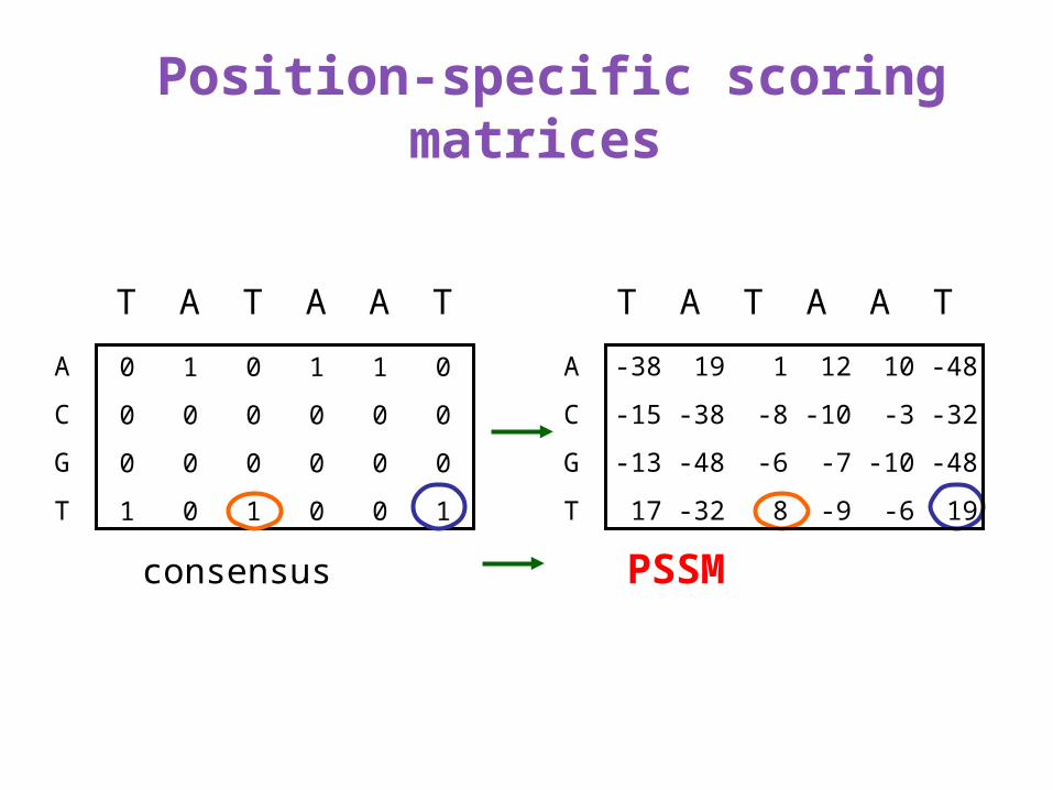
Position-specific scoring matrices
-38 19 1 12 10 -48
-15 -38 -8 -10 -3 -32
-13 -48 -6 -7 -10 -48
17 -32 8 -9 -6 19
0 1 0 1 1 0
0 0 0 0 0 0
0 0 0 0 0 0
1 0 1 0 0 1
A
C
G
T
consensus PSSM
T A T A A T
A
C
G
T
T A T A A T
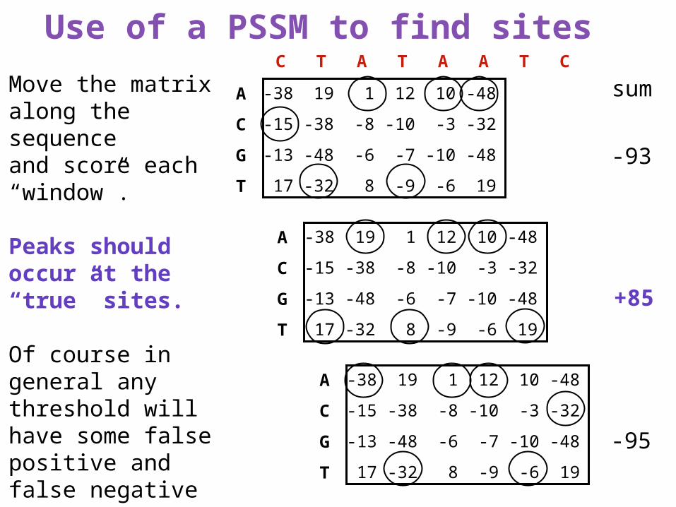
Use of a PSSM to find sites C T A T A A T C
-38 19 1 12 10 -48
-15 -38 -8 -10 -3 -32
-13 -48 -6 -7 -10 -48
17 -32 8 -9 -6 19
A
C
G
T
-38 19 1 12 10 -48
-15 -38 -8 -10 -3 -32
-13 -48 -6 -7 -10 -48
17 -32 8 -9 -6 19
A
C
G
T
-38 19 1 12 10 -48
-15 -38 -8 -10 -3 -32
-13 -48 -6 -7 -10 -48
17 -32 8 -9 -6 19
A
C
G
T
sum
-93
+85
-95
Move the matrixalong the sequenceand score each “window”.
Peaks should occur at the “true” sites.
Of course in general any threshold will have some false positive and false negative rate.

Calculation of a PSSM from counts
0.04 0.88 0.26 0.59 0.49 0.03
0.09 0.03 0.11 0.13 0.22 0.05
0.07 0.01 0.12 0.16 0.12 0.02
0.80 0.08 0.51 0.13 0.18 0.89
9 214 63 142 118 8
22 7 26 31 52 13
18 2 29 38 29 5
193 19 124 31 43 216
A
C
G
T
A
C
G
T
-2.76 1.82 0.06 1.23 0.96 -2.92
-1.46 -3.11 -1.22 -1.00 -0.22 -2.21
-1.76 -5.00 -1.06 -0.67 -1.06 -3.58
1.67 -1.66 1.04 -1.00 -0.49 1.84
A
C
G
T
2
1
01 2 3 4 5 6
Counts from 242 known sites Relative frequencies: fbl
PSSM: log fbl/pb Informativeness: 2+∑bpbllog2pbl

Derivation of PSSM entries
Candidate sequence CTATAATC....
Aligned position 123456
Hypotheses:S=site (and independence)
R=random (equiprobable, independence)
log2 = log2
= (2+log2.09)+...+(2+log2.01)
=
More generally, PSSM score sbl = log fbl/pb
pr(CTATAA | S)
pr(CTATAA | R)
⎛ ⎝ ⎜ ⎞
⎠
€
.09x.03x.26x.13x.51x.01.25x.25x.25x.25x.25x.25
⎛ ⎝
⎞ ⎠
1
10-15 - 32 +1 - 9 +10 - 48{ }
l=position, b=base
pb=background frequency
Suppose that we have aligned sequence data on a number of instances of a given type of site.

Representation of motifs: further steps
Missing from the position-specific distribution
representation of motifs are good ways of dealing with:
Length distributions for insertions/deletions
Cross-position association of amino acids
Hidden Markov models help with the first. The second remains a hard unsolved problem.

Hidden Markov models
Processes {(St,Ot), t=1,…}, where St is the hidden
state and Ot the observation at time t, such that
pr(St | St-1,Ot-1,St-2 ,Ot-2 …) = pr(St | St-1)
pr(Ot | St-1,Ot-1,St-2 ,Ot-2 …) = pr(Ot | St, St-1)
The basics of HMMs were laid bare in a series of beautiful papers by L E Baum and colleagues around 1970, and their formulation has been used almost unchanged to this day.

Hidden Markov models:extensions
Many variants are now used. For example, the distribution of O may not depend on previous S but on previous O values,
pr(Ot | St , St-1 , Ot-1 ,.. ) = pr(Ot | St ), or
pr(Ot | St , St-1 , Ot-1 ,.. ) = pr(Ot | St , St-1 ,Ot-1) .
Most importantly for us, the times of S and O may be decoupled,
permitting the Observation corresponding to State time t to be a string whose length and composition depends on St (and possibly St-1 and part or all of the previous Observations). This is called a hidden semi-Markov or generalized hidden Markov model.

A simple HMM
bA(i) =1/ 6
bB(i) =1/ 4
π =(πA,πB)Initial distribution:
A B
PAB
PBA
PBB
PAA
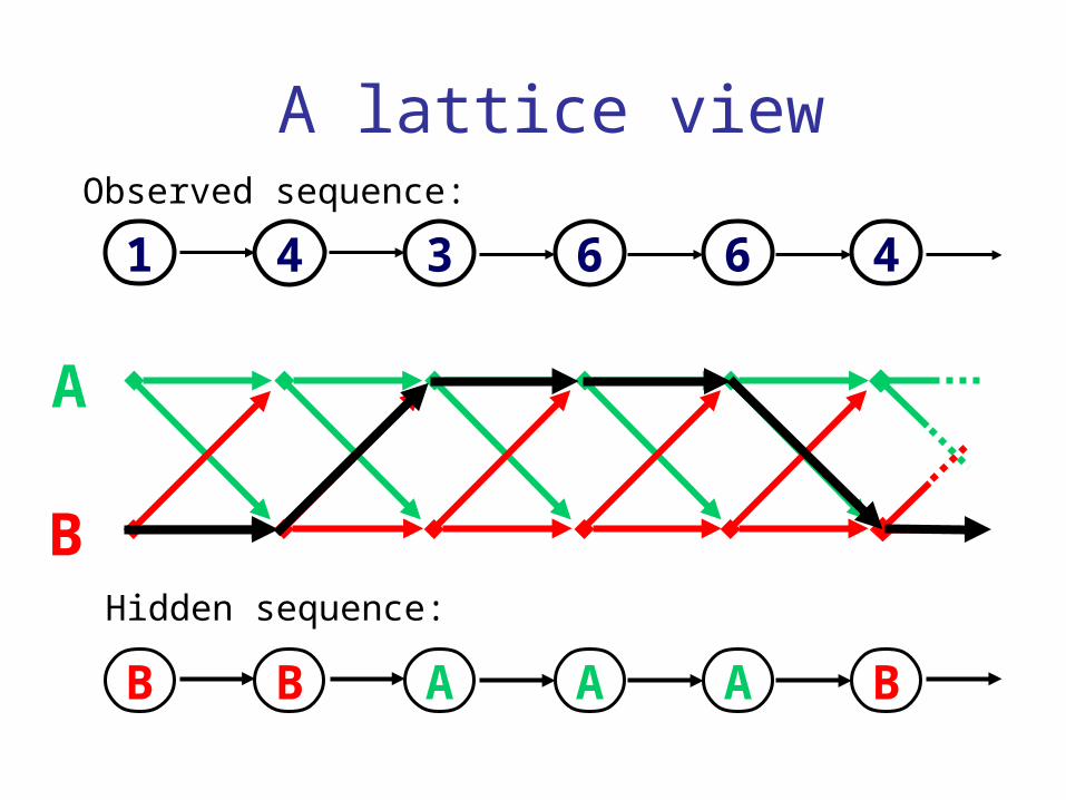
A lattice view
A
B
1 4 3 6 6 4Observed sequence:
BA A ABB
Hidden sequence:

Observed:1,4,3,6,6,4...
A B
Questions:1. What is the most likely die sequence?
2. What is the probability of the observed sequence?
3. What is the probability that the 3rd state is B, given the observed sequence?

The HMM algorithms
Questions:1. What is the most likely die sequence? Viterbi
2. What is the probability of the observed sequence? Forward
3. What is the probability that the 3rd state is B, given the observed sequence? Backward
Forward: (i) = P(observed sequence, ending in state i at base t)
Backward: ß (i) = P(obs. after t | ending in state i at base t)
Viterbi: (i) = max P(obs. , ending in state i at base t)
t
t
t

The forward algorithm
(i) = P(observed sequence, ending in state i at base t)t
αt(j) =( αt−1(i)i=1
N∑ pij)bj (Yt)
αt(j) =( αt−1(i)i=1
N∑ pij)bj (Yt)
αt(j) =( αt−1(i)i=1
N∑ pij)bj (Yt)(i)
T= P(observed sequence)
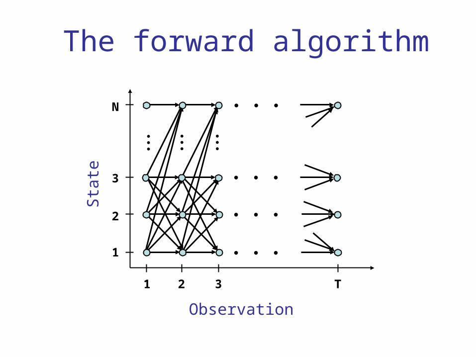
1 2 3 T
1
2
3
N
Observation
Sta
te
The forward algorithm

Some current applications of HMMs to biology
mapping chromosomes
aligning biological sequences
predicting sequence structure
inferring evolutionary relationships
finding genes in DNA sequence
Some early applications of HMMs
finance, but we never saw them
speech recognition
modelling ion channels
In the mid-late 1980s HMMs entered genetics and molecular biology, and they are now firmly entrenched.

Profile HMM: m=match state, I-insert state, d=delete state; go from left to right. I and m states output amino acids; d states are ‘silent”.
d1 d2 d3 d4
I0 I2 I3 I4I1
m0 m1 m2 m3 m4 m5
Start End

Pfam domain-HMMs
Pfam is a library of models of recurrent protein “domains”. They are constructed semi-automatically using hidden Markov models (HMMs).
Pfam families have permanent accession numbers and contain functional annotation and cross-references to other databases, while Pfam-B families are re-generated at each release and are unannotated. See http://www.sanger.ac.uk/Software/Pfam/ http://www.cgr.ki.se/Pfam/ http://pfam.wustl.edu/ http://pfam.jouy.inra.fr/

Finding genes in DNA sequence
This is one of the most challenging and interesting problems in computational biology at the moment. With so many genomes being sequenced so rapidly, it remains important to begin by identifying genes computationally.
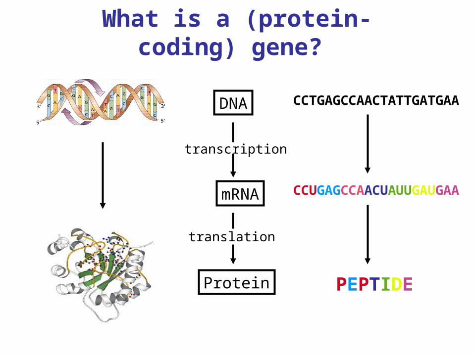
What is a (protein-coding) gene?
Protein
mRNA
DNA
transcription
translation
CCTGAGCCAACTATTGATGAA
PEPTIDE
CCUGAGCCAACUAUUGAUGAA

What is a gene, ctd?
In general the transcribed sequence is longer than the translated portion: parts called introns (intervening sequence) are removed, leaving exons (expressed sequence), and yet other regions remain untranslated. The translated sequence comes in triples called codons, beginning and ending with a unique start (ATG) and one of three stop (TAA, TAG, TGA) codons.
There are also characteristic intron-exon boundaries called splice donor and acceptor sites, and a variety of other motifs: promoters, transcription start sites, polyA sites,branching sites, and so on.
All of the foregoing have statistical characterizations.
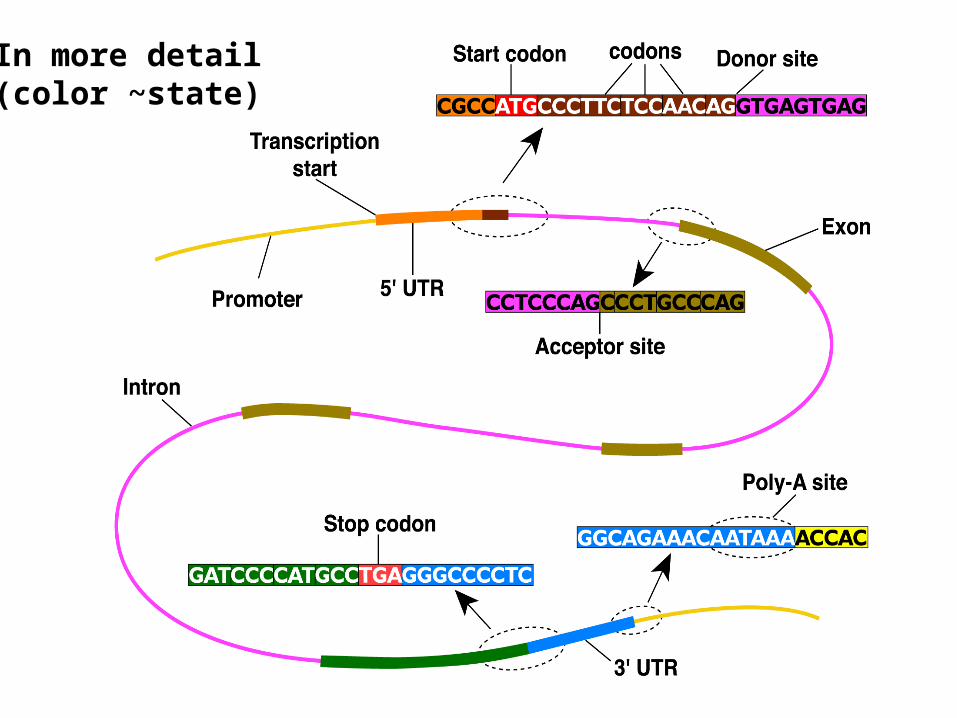
In more detail(color ~state)

Some facts about human genes
Comprise about 3% of the genome
Average gene length: ~ 8,000 bp
Average of 5-6 exons/gene
Average exon length: ~200 bp
Average intron length: ~2,000 bp
~8% genes have a single exon
Some exons can be as small as 1 or 3 bp.
HUMFMR1S is not atypical: 17 exons 40-60 bp long, comprising 3% of a 67,000 bp gene
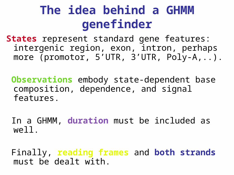
The idea behind a GHMM genefinder
States represent standard gene features: intergenic region, exon, intron, perhaps more (promotor, 5’UTR, 3’UTR, Poly-A,..).
Observations embody state-dependent base composition, dependence, and signal features.
In a GHMM, duration must be included as well. Finally, reading frames and both strands must
be dealt with.
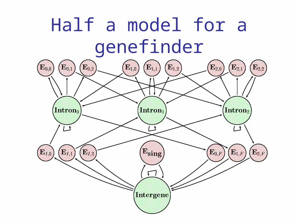
Half a model for a genefinder

Splice sites can be included in the exons

Beyond position-specific distributions
The bases in splice sites exhibit dependence, and not simply of the nearest neighbor kind.
High-order (non-stationary) Markov models would be one option, but the number of parameters in
relation to the amount of data rules them out. The class of variable length Markov models (VLMMs) deriving from early research by Rissanen prove to be valuable in this context. However, there is
likely to be room for more research here.

E0 E1 E2
E
poly-A
3'UTR5'UTR
tEi
Es
I0 I 1 I 2
intergenicregion
Forward (+) strand
Reverse (-) strand
Forward (+) strand
Reverse (-) strand
promoter
62001 AGGACAGGTA CGGCTGTCAT CACTTAGACC TCACCCTGTG GAGCCACACC
62051 CTAGGGTTGG CCAATCTACT CCCAGGAGCA GGGAGGGCAG GAGCCAGGGC
62101 TGGGCATAAA AGTCAGGGCA GAGCCATCTA TTGCTTACAT TTGCTTCTGA
62151 CACAACTGTG TTCACTAGCA ACCTCAAACA GACACCATGG TGCACCTGAC
62201 TCCTGAGGAG AAGTCTGCCG TTACTGCCCT GTGGGGCAAG GTGAACGTGG
62251 ATGAAGTTGG TGGTGAGGCC CTGGGCAGGT TGGTATCAAG GTTACAAGAC
62301 AGGTTTAAGG AGACCAATAG AAACTGGGCA TGTGGAGACA GAGAAGACTC
62351 TTGGGTTTCT GATAGGCACT GACTCTCTCT GCCTATTGGT CTATTTTCCC
62401 ACCCTTAGGC TGCTGGTGGT CTACCCTTGG ACCCAGAGGT TCTTTGAGTC
62451 CTTTGGGGAT CTGTCCACTC CTGATGCTGT TATGGGCAAC CCTAAGGTGA
62501 AGGCTCATGG CAAGAAAGTG CTCGGTGCCT TTAGTGATGG CCTGGCTCAC
62551 CTGGACAACC TCAAGGGCAC CTTTGCCACA CTGAGTGAGC TGCACTGTGA
62601 CAAGCTGCAC GTGGATCCTG AGAACTTCAG GGTGAGTCTA TGGGACCCTT
62651 GATGTTTTCT TTCCCCTTCT TTTCTATGGT TAAGTTCATG TCATAGGAAG
62701 GGGAGAAGTA ACAGGGTACA GTTTAGAATG GGAAACAGAC GAATGATTGC
62751 ATCAGTGTGG AAGTCTCAGG ATCGTTTTAG TTTCTTTTAT TTGCTGTTCA
62801 TAACAATTGT TTTCTTTTGT TTAATTCTTG CTTTCTTTTT TTTTCTTCTC
62851 CGCAATTTTT ACTATTATAC TTAATGCCTT AACATTGTGT ATAACAAAAG
62901 GAAATATCTC TGAGATACAT TAAGTAACTT AAAAAAAAAC TTTACACAGT
62951 CTGCCTAGTA CATTACTATT TGGAATATAT GTGTGCTTAT TTGCATATTC
63001 ATAATCTCCC TACTTTATTT TCTTTTATTT TTAATTGATA CATAATCATT
63051 ATACATATTT ATGGGTTAAA GTGTAATGTT TTAATATGTG TACACATATT
63101 GACCAAATCA GGGTAATTTT GCATTTGTAA TTTTAAAAAA TGCTTTCTTC
63151 TTTTAATATA CTTTTTTGTT TATCTTATTT CTAATACTTT CCCTAATCTC
63201 TTTCTTTCAG GGCAATAATG ATACAATGTA TCATGCCTCT TTGCACCATT
63251 CTAAAGAATA ACAGTGATAA TTTCTGGGTT AAGGCAATAG CAATATTTCT
63301 GCATATAAAT ATTTCTGCAT ATAAATTGTA ACTGATGTAA GAGGTTTCAT
63351 ATTGCTAATA GCAGCTACAA TCCAGCTACC ATTCTGCTTT TATTTTATGG
63401 TTGGGATAAG GCTGGATTAT TCTGAGTCCA AGCTAGGCCC TTTTGCTAAT
63451 CATGTTCATA CCTCTTATCT TCCTCCCACA GCTCCTGGGC AACGTGCTGG
63501 TCTGTGTGCT GGCCCATCAC TTTGGCAAAG AATTCACCCC ACCAGTGCAG
63551 GCTGCCTATC AGAAAGTGGT GGCTGGTGTG GCTAATGCCC TGGCCCACAA
63601 GTATCACTAA GCTCGCTTTC TTGCTGTCCA ATTTCTATTA AAGGTTCCTT
63651 TGTTCCCTAA GTCCAACTAC TAAACTGGGG GATATTATGA AGGGCCTTGA
63701 GCATCTGGAT TCTGCCTAAT AAAAAACATT TATTTTCATT GCAATGATGT
GENSCAN (Burge & Karlin)

Remark
In general the problem of identifying (annotating) human genes is considerably harder than ß-globin might suggest.
The human factor VIII gene (whose mutations cause hemophilia A) is spread over ~186,000 bp. It consists of 26 exons ranging in size from 69 to 3,106 bp, and its 25 introns range in size from 207 to 32,400 bp. The complete gene is thus ~9 kb of exon and ~177 kb of intron.
The biggest human gene yet is for dystrophin. It has
> 30 exons and is spread over 2.4 million bp.

Challenges in the analysis of sequence data
Understanding the biology well enough to begin.
Designing HMM architecture, e.g. in Marcoil for coiled-coils.
Modelling the parts, e.g. VLMMs for splice sites.
Coding = software engineering, is the hardest and most important task of all: making it all work.
Obtaining good data sets for use in careful evaluation and comparison with competing algorithms; designing the studies.
Opportunities for methodological research.
Topics not mentioned include
Molecular evolution, including phylogenetic inference (building trees from aligned sequence data)
Sequence alignment (pairwise, multiple), including use of Gibbs sampler
Stochastic context-free grammar models and the analysis of RNA sequence data.

Acknowledgements
Mauro Delorenzi (WEHI)
Simon Cawley (Affymetrix)
Tony Wirth (CS, Princeton)
Lior Pachter (Math, UCB)
Marina Alexandersson (Stat, UCB)
ReferencesBiological Sequence AnalysisR Durbin, S Eddy, A Krogh and G MitchisonCambridge University Press, 1998.
Bioinformatics The machine learning approach
P Baldi and S BrunakThe MIT Press, 1998
Post-Genome InformaticsM KanehisaOxford University Press, 2000
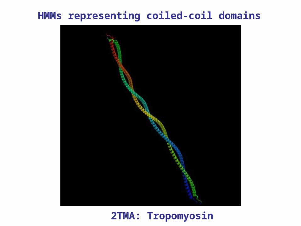
2TMA: Tropomyosin
HMMs representing coiled-coil domains

Coiled-coil domains, schematically
dimeric parallel helices, heptad repeats, knobs-into-holes
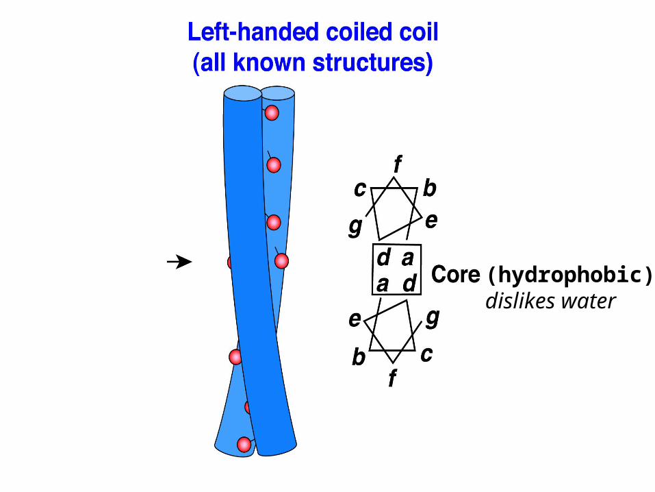
(hydrophobic)dislikes water
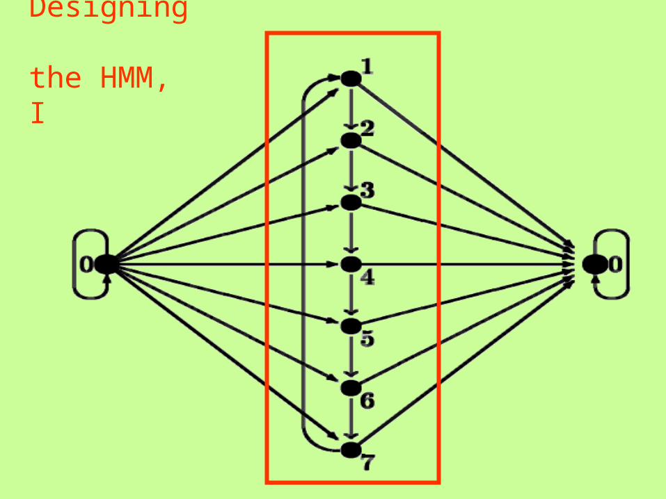
Designing the HMM, I

Designingthe HMM, 2

Designing the HMM, 3

HMM: decoding
WGP ARQLNES VKDINKM LER HPBBB CCCCCCC CCCCCCC CCC BB000 abcdefg abcdefg abc 0000c defgabc defgabc def g0
Sequence Labels Path1 Path2
VITERBI decoding: of all possible state-paths, we determine the maximum probability one given the amino acid sequence O;
POSTERIOR decoding: at each position, we determine the state with the highest probability given O.
Issue: how to measure the strength of a potential CC domain, and how should this depend on the length of a domain?

CC-PROBABILITY PROFILE
Fusion protein of simian parainfluenza virus 5
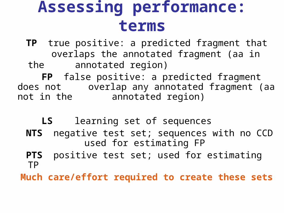
Assessing performance: terms
TP true positive: a predicted fragment that overlaps the annotated fragment (aa in the
annotated region) FP false positive: a predicted fragment does not
overlap any annotated fragment (aa not in the annotated region)
LS learning set of sequences
NTS negative test set; sequences with no CCD used for estimating FP
PTS positive test set; used for estimating TPMuch care/effort required to create these sets

Assessing performance: study design Study the variability of performance under variation of the sequences used for determining
the model parameters.
Compare methods using the same set of aa-frequencies / emission probabilities. Use the same set of domains for learning and testing instead of testing on different protein
families.
Choose a number of FP-rates and calculate the corresponding TP-rates (ROC curve).

PTS subdivided 150 times at random (stratified)into 2/3 for learning and the rest for testing.
ANALYSIS OF RESULTS
LEARNING PHASE => PARAMETERS
TESTING ON NTS => THRESHOLDS
TESTING ON PTS => TP-VALUES
150 X

Assessing performance: summaries
TP-rate at given FP-rate: per family / per length-class
TP- and FP-rates for aa’s: per family / per length-class
Accuracy: at the borders and of length prediction
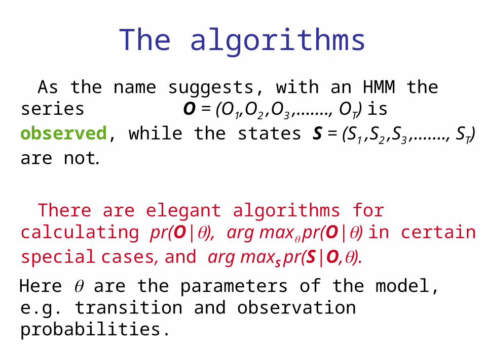
The algorithms
As the name suggests, with an HMM the series O = (O1,O2 ,O3 ,……., OT) is observed, while the states S = (S1 ,S2 ,S3 ,……., ST) are not.
There are elegant algorithms for calculating pr(O|), arg max pr(O|) in certain special cases, and arg maxS pr(S|O,).
Here are the parameters of the model, e.g. transition and observation probabilities.