San Jose State University San Jose State University

SJSU ScholarWorks SJSU ScholarWorks

Master's Projects Master's Theses and Graduate Research

Fall 12-17-2020

Bioinformatics Metadata Extraction for Machine Learning Bioinformatics Metadata Extraction for Machine Learning

Analysis Analysis

Zachary Tom San Jose State University

Follow this and additional works at: https://scholarworks.sjsu.edu/etd_projects

Part of the Artificial Intelligence and Robotics Commons, and the Bioinformatics Commons

Recommended Citation Recommended Citation Tom, Zachary, "Bioinformatics Metadata Extraction for Machine Learning Analysis" (2020). Master's Projects. 964. DOI: https://doi.org/10.31979/etd.s3ta-b264 https://scholarworks.sjsu.edu/etd_projects/964

This Master's Project is brought to you for free and open access by the Master's Theses and Graduate Research at SJSU ScholarWorks. It has been accepted for inclusion in Master's Projects by an authorized administrator of SJSU ScholarWorks. For more information, please contact scholarworks@sjsu.edu.

Bioinformatics Metadata Extraction for Machine Learning Analysis

A Project

Presented to

The Faculty of the Department of Computer Science

San Jose State University

In Partial Fulfillment

of the Requirements for the Degree

Master of Science

by

Zachary Tom

December 2020

© 2020

Zachary Tom

ALL RIGHTS RESERVED

The Designated Project Committee Approves the Project Titled

Bioinformatics Metadata Extraction for Machine Learning Analysis

by

Zachary Tom

APPROVED FOR THE DEPARTMENT OF COMPUTER SCIENCE

SAN JOSE STATE UNIVERSITY

December 2020

Wendy Lee, Ph.D. Department of Computer Science

Fabio Di Troia, Ph.D. Department of Computer Science

William Andreopoulos, Ph.D. Department of Computer Science

ABSTRACT

Bioinformatics Metadata Extraction for Machine Learning Analysis

by Zachary Tom

Next generation sequencing (NGS) has revolutionized the biological sciences. Today,

entire genomes can be rapidly sequenced, enabling advancements in personalized medicine,

genetic diseases, and more. The National Center for Biotechnology Information (NCBI)

hosts the Sequence Read Archive (SRA) containing vast amounts of valuable NGS data.

Recently, research has shown that sequencing errors in conventional NGS workflows are

key confounding factors for detecting mutations. Various steps such as sample handling

and library preparation can introduce artifacts that affect the accuracy of calling rare

mutations. Thus, there is a need for more insight into the exact relationship between

various steps of the NGS workflow- the metadata- and sequencing artifacts. This paper

presents a new tool called SRAMetadataX that enables researchers to easily extract crucial

metadata from SRA submissions. The tool was used to identify eight sequencing runs that

utilized hybrid capture or PCR for enrichment. A bioinformatics pipeline was built that

identified 298,936 potential sequencing artifacts from the runs. Various machine learning

models were trained on the data, and results showed that the models were able to predict

enrichment method with about 70% accuracy, indicating that different enrichment methods

likely produce specific sequencing artifacts.

ACKNOWLEDGMENTS

I would like to thank my advisor Dr. Wendy Lee for her invaluable guidance and

continuous support throughout the development of this project. I also extend my gratitude

to Dr. Fabio Di Troia and Dr. William Andreopoulos for their advice and feedback. Finally,

I would like to thank my girlfriend, family, and friends for their constant support and

encouragement throughout my academic endeavour.

v

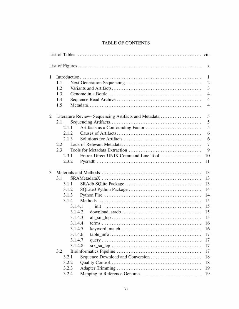
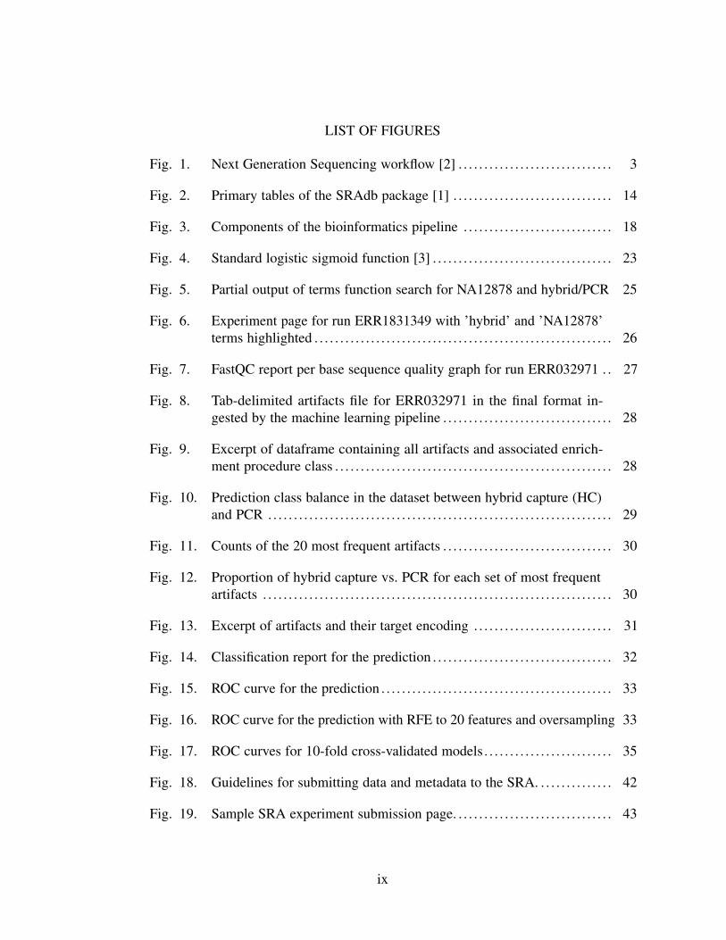
TABLE OF CONTENTS

List of Tables . . . . . . . . . . . . . . . . . . . . . . . . . . . . . . . . . . . . . . . . . . . . . . . . . . . . . . . . . . . . . . . . . . . . . . . . . . viii

List of Figures . . . . . . . . . . . . . . . . . . . . . . . . . . . . . . . . . . . . . . . . . . . . . . . . . . . . . . . . . . . . . . . . . . . . . . . . . x

1 Introduction. . . . . . . . . . . . . . . . . . . . . . . . . . . . . . . . . . . . . . . . . . . . . . . . . . . . . . . . . . . . . . . . . . . . . . . . 11.1 Next Generation Sequencing . . . . . . . . . . . . . . . . . . . . . . . . . . . . . . . . . . . . . . . . . . . . . 21.2 Variants and Artifacts. . . . . . . . . . . . . . . . . . . . . . . . . . . . . . . . . . . . . . . . . . . . . . . . . . . . . 31.3 Genome in a Bottle . . . . . . . . . . . . . . . . . . . . . . . . . . . . . . . . . . . . . . . . . . . . . . . . . . . . . . . 41.4 Sequence Read Archive . . . . . . . . . . . . . . . . . . . . . . . . . . . . . . . . . . . . . . . . . . . . . . . . . . 41.5 Metadata. . . . . . . . . . . . . . . . . . . . . . . . . . . . . . . . . . . . . . . . . . . . . . . . . . . . . . . . . . . . . . . . . . . 4

2 Literature Review- Sequencing Artifacts and Metadata . . . . . . . . . . . . . . . . . . . . . . . . 52.1 Sequencing Artifacts. . . . . . . . . . . . . . . . . . . . . . . . . . . . . . . . . . . . . . . . . . . . . . . . . . . . . . 5

2.1.1 Artifacts as a Confounding Factor . . . . . . . . . . . . . . . . . . . . . . . . . . . . . . . . . 52.1.2 Causes of Artifacts . . . . . . . . . . . . . . . . . . . . . . . . . . . . . . . . . . . . . . . . . . . . . . . . . . 62.1.3 Solutions for Artifacts . . . . . . . . . . . . . . . . . . . . . . . . . . . . . . . . . . . . . . . . . . . . . . 6

2.2 Lack of Relevant Metadata . . . . . . . . . . . . . . . . . . . . . . . . . . . . . . . . . . . . . . . . . . . . . . . 72.3 Tools for Metadata Extraction . . . . . . . . . . . . . . . . . . . . . . . . . . . . . . . . . . . . . . . . . . . 9

2.3.1 Entrez Direct UNIX Command Line Tool . . . . . . . . . . . . . . . . . . . . . . . . 102.3.2 Pysradb . . . . . . . . . . . . . . . . . . . . . . . . . . . . . . . . . . . . . . . . . . . . . . . . . . . . . . . . . . . . . . 11

3 Materials and Methods . . . . . . . . . . . . . . . . . . . . . . . . . . . . . . . . . . . . . . . . . . . . . . . . . . . . . . . . . . . 133.1 SRAMetadataX . . . . . . . . . . . . . . . . . . . . . . . . . . . . . . . . . . . . . . . . . . . . . . . . . . . . . . . . . . . 13

3.1.1 SRAdb SQlite Package . . . . . . . . . . . . . . . . . . . . . . . . . . . . . . . . . . . . . . . . . . . . . 133.1.2 SQLite3 Python Package . . . . . . . . . . . . . . . . . . . . . . . . . . . . . . . . . . . . . . . . . . . 143.1.3 Python Fire . . . . . . . . . . . . . . . . . . . . . . . . . . . . . . . . . . . . . . . . . . . . . . . . . . . . . . . . . . 143.1.4 Methods . . . . . . . . . . . . . . . . . . . . . . . . . . . . . . . . . . . . . . . . . . . . . . . . . . . . . . . . . . . . . 15

3.1.4.1 init . . . . . . . . . . . . . . . . . . . . . . . . . . . . . . . . . . . . . . . . . . . . . . . . . . . . . . . . 153.1.4.2 download sradb . . . . . . . . . . . . . . . . . . . . . . . . . . . . . . . . . . . . . . . . . . . . . . . 153.1.4.3 all sm lcp . . . . . . . . . . . . . . . . . . . . . . . . . . . . . . . . . . . . . . . . . . . . . . . . . . . . . 153.1.4.4 terms . . . . . . . . . . . . . . . . . . . . . . . . . . . . . . . . . . . . . . . . . . . . . . . . . . . . . . . . . . . 163.1.4.5 keyword match. . . . . . . . . . . . . . . . . . . . . . . . . . . . . . . . . . . . . . . . . . . . . . . . 163.1.4.6 table info . . . . . . . . . . . . . . . . . . . . . . . . . . . . . . . . . . . . . . . . . . . . . . . . . . . . . . 173.1.4.7 query . . . . . . . . . . . . . . . . . . . . . . . . . . . . . . . . . . . . . . . . . . . . . . . . . . . . . . . . . . . 173.1.4.8 srx sa lcp . . . . . . . . . . . . . . . . . . . . . . . . . . . . . . . . . . . . . . . . . . . . . . . . . . . . . 17

3.2 Bioinformatics Pipeline . . . . . . . . . . . . . . . . . . . . . . . . . . . . . . . . . . . . . . . . . . . . . . . . . . 173.2.1 Sequence Download and Conversion . . . . . . . . . . . . . . . . . . . . . . . . . . . . . . 183.2.2 Quality Control. . . . . . . . . . . . . . . . . . . . . . . . . . . . . . . . . . . . . . . . . . . . . . . . . . . . . . 183.2.3 Adapter Trimming . . . . . . . . . . . . . . . . . . . . . . . . . . . . . . . . . . . . . . . . . . . . . . . . . . 193.2.4 Mapping to Reference Genome . . . . . . . . . . . . . . . . . . . . . . . . . . . . . . . . . . . . 19

vi

3.2.5 Variant Calling . . . . . . . . . . . . . . . . . . . . . . . . . . . . . . . . . . . . . . . . . . . . . . . . . . . . . . 193.2.6 Variant Filtering . . . . . . . . . . . . . . . . . . . . . . . . . . . . . . . . . . . . . . . . . . . . . . . . . . . . . 19

3.3 Machine Learning Pipeline. . . . . . . . . . . . . . . . . . . . . . . . . . . . . . . . . . . . . . . . . . . . . . . 203.3.1 Data Description . . . . . . . . . . . . . . . . . . . . . . . . . . . . . . . . . . . . . . . . . . . . . . . . . . . . 203.3.2 Data Pre-Processing . . . . . . . . . . . . . . . . . . . . . . . . . . . . . . . . . . . . . . . . . . . . . . . . 213.3.3 Data Evaluation . . . . . . . . . . . . . . . . . . . . . . . . . . . . . . . . . . . . . . . . . . . . . . . . . . . . . 213.3.4 Baseline Model. . . . . . . . . . . . . . . . . . . . . . . . . . . . . . . . . . . . . . . . . . . . . . . . . . . . . . 223.3.5 Performance Evaluation . . . . . . . . . . . . . . . . . . . . . . . . . . . . . . . . . . . . . . . . . . . . 23

4 Results . . . . . . . . . . . . . . . . . . . . . . . . . . . . . . . . . . . . . . . . . . . . . . . . . . . . . . . . . . . . . . . . . . . . . . . . . . . . . 254.1 SRAMetadataX Performance . . . . . . . . . . . . . . . . . . . . . . . . . . . . . . . . . . . . . . . . . . . . 254.2 Identifying Artifacts . . . . . . . . . . . . . . . . . . . . . . . . . . . . . . . . . . . . . . . . . . . . . . . . . . . . . . 264.3 Application of Machine Learning . . . . . . . . . . . . . . . . . . . . . . . . . . . . . . . . . . . . . . . 28

4.3.1 Data Pre-Processing . . . . . . . . . . . . . . . . . . . . . . . . . . . . . . . . . . . . . . . . . . . . . . . . 284.3.2 Data Exploration . . . . . . . . . . . . . . . . . . . . . . . . . . . . . . . . . . . . . . . . . . . . . . . . . . . . 294.3.3 Encoding . . . . . . . . . . . . . . . . . . . . . . . . . . . . . . . . . . . . . . . . . . . . . . . . . . . . . . . . . . . . 314.3.4 Model Training and Prediction . . . . . . . . . . . . . . . . . . . . . . . . . . . . . . . . . . . . . 314.3.5 Performance Evaluation . . . . . . . . . . . . . . . . . . . . . . . . . . . . . . . . . . . . . . . . . . . . 314.3.6 Experiment 2 . . . . . . . . . . . . . . . . . . . . . . . . . . . . . . . . . . . . . . . . . . . . . . . . . . . . . . . . 324.3.7 Experiment 3 . . . . . . . . . . . . . . . . . . . . . . . . . . . . . . . . . . . . . . . . . . . . . . . . . . . . . . . . 34

5 Conclusion and Future Work . . . . . . . . . . . . . . . . . . . . . . . . . . . . . . . . . . . . . . . . . . . . . . . . . . . . . 365.1 Conclusion . . . . . . . . . . . . . . . . . . . . . . . . . . . . . . . . . . . . . . . . . . . . . . . . . . . . . . . . . . . . . . . . 365.2 Future Work . . . . . . . . . . . . . . . . . . . . . . . . . . . . . . . . . . . . . . . . . . . . . . . . . . . . . . . . . . . . . . . 36

References . . . . . . . . . . . . . . . . . . . . . . . . . . . . . . . . . . . . . . . . . . . . . . . . . . . . . . . . . . . . . . . . . . . . . . . . . . . . . 38

Appendix A: Sequence Read Archive . . . . . . . . . . . . . . . . . . . . . . . . . . . . . . . . . . . . . . . . . . . . . . . 42A.1 SRA Submission Guidelines . . . . . . . . . . . . . . . . . . . . . . . . . . . . . . . . . . . . . . . . . . . . . 42A.2 SRA Experiment Page . . . . . . . . . . . . . . . . . . . . . . . . . . . . . . . . . . . . . . . . . . . . . . . . . . . . 43

Appendix B: SRAMetadataX Function Output . . . . . . . . . . . . . . . . . . . . . . . . . . . . . . . . . . . . . 44B.1 download sradb. . . . . . . . . . . . . . . . . . . . . . . . . . . . . . . . . . . . . . . . . . . . . . . . . . . . . . . . . . . 44B.2 all sm lcp . . . . . . . . . . . . . . . . . . . . . . . . . . . . . . . . . . . . . . . . . . . . . . . . . . . . . . . . . . . . . . . . . 44B.3 query. . . . . . . . . . . . . . . . . . . . . . . . . . . . . . . . . . . . . . . . . . . . . . . . . . . . . . . . . . . . . . . . . . . . . . . 44B.4 srx sa lcp . . . . . . . . . . . . . . . . . . . . . . . . . . . . . . . . . . . . . . . . . . . . . . . . . . . . . . . . . . . . . . . . . 44B.5 table info . . . . . . . . . . . . . . . . . . . . . . . . . . . . . . . . . . . . . . . . . . . . . . . . . . . . . . . . . . . . . . . . . . 44B.6 terms . . . . . . . . . . . . . . . . . . . . . . . . . . . . . . . . . . . . . . . . . . . . . . . . . . . . . . . . . . . . . . . . . . . . . . . 44

vii

viii

LIST OF TABLES

Table 1. Protocol steps keywords [1] . . . . . . . . . . . . . . . . . . . . . . . . . . . . . . . . . . . . . . . . . . . . . . 8

Table 2. SRAdb query results [1] . . . . . . . . . . . . . . . . . . . . . . . . . . . . . . . . . . . . . . . . . . . . . . . . . . 9

Table 3. Runinfo metadata table fields searched . . . . . . . . . . . . . . . . . . . . . . . . . . . . . . . . . . 10

Table 4. pysradb metadata fields . . . . . . . . . . . . . . . . . . . . . . . . . . . . . . . . . . . . . . . . . . . . . . . . . . . 11

Table 5. Chosen SRA run accessions . . . . . . . . . . . . . . . . . . . . . . . . . . . . . . . . . . . . . . . . . . . . . . 26

Table 6. Confusion Matrix . . . . . . . . . . . . . . . . . . . . . . . . . . . . . . . . . . . . . . . . . . . . . . . . . . . . . . . . . 32

ix

LIST OF FIGURES

Fig. 1. Next Generation Sequencing workflow [2] . . . . . . . . . . . . . . . . . . . . . . . . . . . . . . 3

Fig. 2. Primary tables of the SRAdb package [1] . . . . . . . . . . . . . . . . . . . . . . . . . . . . . . . 14

Fig. 3. Components of the bioinformatics pipeline . . . . . . . . . . . . . . . . . . . . . . . . . . . . . 18

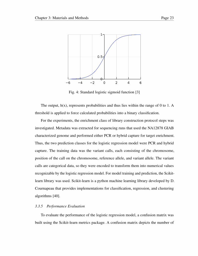
Fig. 4. Standard logistic sigmoid function [3] . . . . . . . . . . . . . . . . . . . . . . . . . . . . . . . . . . . 23

Fig. 5. Partial output of terms function search for NA12878 and hybrid/PCR 25

Fig. 6. Experiment page for run ERR1831349 with ’hybrid’ and ’NA12878’terms highlighted . . . . . . . . . . . . . . . . . . . . . . . . . . . . . . . . . . . . . . . . . . . . . . . . . . . . . . . . . . 26

Fig. 7. FastQC report per base sequence quality graph for run ERR032971 . . 27

Fig. 8. Tab-delimited artifacts file for ERR032971 in the final format in-gested by the machine learning pipeline . . . . . . . . . . . . . . . . . . . . . . . . . . . . . . . . . 28

Fig. 9. Excerpt of dataframe containing all artifacts and associated enrich-ment procedure class . . . . . . . . . . . . . . . . . . . . . . . . . . . . . . . . . . . . . . . . . . . . . . . . . . . . . . 28

Fig. 10. Prediction class balance in the dataset between hybrid capture (HC)and PCR . . . . . . . . . . . . . . . . . . . . . . . . . . . . . . . . . . . . . . . . . . . . . . . . . . . . . . . . . . . . . . . . . . . 29

Fig. 11. Counts of the 20 most frequent artifacts . . . . . . . . . . . . . . . . . . . . . . . . . . . . . . . . . 30

Fig. 12. Proportion of hybrid capture vs. PCR for each set of most frequentartifacts . . . . . . . . . . . . . . . . . . . . . . . . . . . . . . . . . . . . . . . . . . . . . . . . . . . . . . . . . . . . . . . . . . . . 30

Fig. 13. Excerpt of artifacts and their target encoding . . . . . . . . . . . . . . . . . . . . . . . . . . . 31

Fig. 14. Classification report for the prediction . . . . . . . . . . . . . . . . . . . . . . . . . . . . . . . . . . . 32

Fig. 15. ROC curve for the prediction . . . . . . . . . . . . . . . . . . . . . . . . . . . . . . . . . . . . . . . . . . . . . 33

Fig. 16. ROC curve for the prediction with RFE to 20 features and oversampling 33

Fig. 17. ROC curves for 10-fold cross-validated models . . . . . . . . . . . . . . . . . . . . . . . . . 35

Fig. 18. Guidelines for submitting data and metadata to the SRA. . . . . . . . . . . . . . . 42

Fig. 19. Sample SRA experiment submission page. . . . . . . . . . . . . . . . . . . . . . . . . . . . . . . 43

x

Fig. 20. SRAdb package download with status bar. . . . . . . . . . . . . . . . . . . . . . . . . . . . . . . 44

Fig. 21. Submissions that used the NA12878 genome, Illumina HiSeq 2000,whole genome sequencing, and PCR, and contain sm/lcp data. . . . . . . . . 44

Fig. 22. Query for metainfo about the SRAdb SQLite database. . . . . . . . . . . . . . . . . 44

Fig. 23. Study abstract/library construction protocol data for SRX7949756and SRX321552. . . . . . . . . . . . . . . . . . . . . . . . . . . . . . . . . . . . . . . . . . . . . . . . . . . . . . . . . . . 45

Fig. 24. Fields of the experiment table. . . . . . . . . . . . . . . . . . . . . . . . . . . . . . . . . . . . . . . . . . . . 45

Fig. 25. Submissions that contain the terms ‘NA12878’ and ‘PCR’. . . . . . . . . . . . . 45

Chapter 1: Introduction Page 1

1 Introduction

In recent years there has been an explosion in genetic research and technologies.

Companies like 23 and Me have grown at incredible rates, in conjunction with a

sudden worldwide fascination with discovering ancestral history and ethnic makeup [4].

Individuals can send a sample of saliva to 23 and Me from which DNA will be extracted

and used to discover a wide range of genetic information. Genetic technologies are

also used to determine diseases that individuals are more susceptible to and to develop

personalized medicine. These advanced insights are made possible through a process

called sequencing.

Sequencing is the technique through which a person’s DNA is read. Original sequenc-

ing methods from the 1980s to early 2000s were slow and expensive. For example,

the Human Genome Project was a worldwide collaboration that for the first time

successfully sequenced a single human genome. While it was an immensely important

and groundbreaking endeavor, it took over 10 years to complete, lasting from 1990 to

2003 [5]. Clearly, there was a need for a faster sequencing technology, and that need was

met through the advent of Next Generation Sequencing in the early 2000s. NGS is a faster

and cheaper sequencing technology, capable of sequencing a human genome in just 24

hours. As a result, through the improved sequencing method of NGS, advancements have

been made in personalized medicine, genetic disease studies, and more [6], [7].

When using NGS for medical and genetic investigation, scientists are typically looking

for mutations, or changes, in DNA. Recently however, research has shown that sequencing

errors, also called artifacts, occur frequently in conventional NGS workflows. These

artifacts are problematic because they appear to be relevant mutations, while in reality

they are artificially produced from steps of the NGS workflow and thus are not relevant.

Consequently, artifacts negatively affect scientists’ ability to detect relevant, naturally

occurring mutations [8] [9]. Various steps of the workflow can introduce these artifacts. For

Chapter 1: Introduction Page 2

example, certain chemical reagents used to extract DNA can cause erroneous mutations to

appear, and some methods for preparing DNA for sequencing can cause oxidation that

also introduces artifacts [7]. It is important for these artifacts to be accurately detected

and removed, because then better personalized medicine can be developed and genetic

diseases can be more efficiently predicted and treated. The important question then is

which steps of the NGS workflow cause which artifacts to occur?

This question can be answered by applying machine learning algorithms to a dataset

consisting of sequencing artifacts and associated metadata that includes sample preparation

techniques and library construction protocol data. However, this specific metadata is not

easy to obtain. Research has shown that out of all submissions in the NCBI SRA, a small

minority report such information. Furthermore, there are no tools capable of extracting the

specific metadata relevant to the sequencing artifacts. In this project, a newly developed

tool called SRAMetadataX is used to extract the metadata. Then, a bioinformatics pipeline

is used to process sequencing data and identifying potential artifacts. Finally, machine

learning is applied to demonstrate how the metadata can be used in conjunction with

variant calling data to elucidate a relationship between the steps of the NGS workflow and

resulting artifacts.

1.1 Next Generation Sequencing

Next generation sequencing is also commonly referred to as massively parallel or deep

sequencing [10]. This is because the cardinal speed of NGS is due in large part to its ability

to parallelize the sequencing process, drastically decreasing the amount of time required

to sequence a sample. Three basic steps define the NGS workflow: library preparation,

sequencing, and data analysis [11]. Library preparation is crucial to success and consists of

DNA or RNA fragmentation, adapter ligation, and amplification/enrichment (Fig. 1). NGS

is also called deep sequencing because genomic regions are sequenced multiple times,

Chapter 1: Introduction Page 3

sometimes hundreds or even thousands of times. Deep sequencing is advantageous in that

it can better detect rare variants, also called single nucleotide polymorphisms (SNPs).

Fig. 1: Next Generation Sequencing workflow [2]

1.2 Variants and Artifacts

Variants are nucleotide substitutions at a specific position in the genome. They are

often SNPs, but only when they are present in 1% or more of a population [12]. Variants

are important because they can affect how an individual responds to drugs and pathogens,

and how they develop diseases. Artifacts on the other hand, are variants introduced by

non-biological processes. They are born from steps of the sequencing workflow, namely

sample manipulation and library construction. Artifacts are harmful in that they, if not

properly identified and accounted for, can detract from the pool of relevant, naturally

occurring variants and mislead analysis [13].

Chapter 1: Introduction Page 4

1.3 Genome in a Bottle

Genome in a Bottle (GIAB) is a consortium hosted by the National Institute of

Standards and Technology that consists of public, private, and academic groups. GIAB has

characterized multiple human genomes for use in benchmarking. By utilizing sequencing

data generated from a wide variety of platforms and technologies, they have identified high

confidence variant calls and regions [14]. These high confidence variants are ones that

developed from natural biological processes, and can be distinguished from sequencing

artifacts. Thus, the GIAB data is essential for identifying potential sequencing artifacts.

1.4 Sequence Read Archive

The SRA is a public database that houses DNA sequencing data, most commonly

generated by NGS through high throughput sequencing [15]. It was established by the

NCBI, and is run in collaboration with the DNA Data Bank of Japan (DDBJ) and the

European Bioinformatics Institute (EBI). Since its inception in 2007, the SRA has seen

rapid growth in volume of data stored and significance among open access journals [16].

Thus, the SRA has been chosen as the primary resource for metadata extraction and

processing for this project.

1.5 Metadata

Various metadata exists for every SRA sequencing run submission. This metadata

accompanies the actual sequencing data, which consists of sequences of nucleotides-

adenine (A), cytosine (C), thymine (T), and guanine (G) - that make up the DNA sample.

Metadata fields include run accession, run date, instrument model, library strategy, sample

ID, and more [15]. The fields that are of most interest, however, are design description,

library strategy, library construction protocol, instrument model, platform parameters,

and study abstract. These fields contain the sample manipulation and library construction

protocol steps (if reported) that can produce sequencing artifacts.

Chapter 2: Related Work Page 5

2 Literature Review- Sequencing Artifacts and Metadata

In the following sections, the ways in which the relationship between steps of the NGS

workflow and consequent sequencing artifacts have been researched are presented. Then,

the dearth of metadata is examined and existing tools are surveyed to show the need for a

tool that can extract relevant metadata.

2.1 Sequencing Artifacts

2.1.1 Artifacts as a Confounding Factor

Sequencing artifacts affect researchers’ ability to accurately identify rare mutations.

They dilute the pool of relevant, biologically occurring mutations with their artificial

origins. There are many ways in which sequencing artifacts have been shown to be

confounding factors. L. Chen et al. [17] discovered that sequencing artifacts decreased

the accuracy of determining low frequency mutations, specifically in tumor-associated

cells. In fact, they discovered that artifacts can make up over 70 percent of all discovered

mutations, thus making conventional methods for identifying mutations inadequate. In

confirmation of L. Chen et al.’s approach, X. Ma et al. [18] tracked the sequencing artifact

rate of specific bases and found a substitution error rate of 10−5 to 10−4. They found that

for nucleotide substitution types of A to C and T to G, error rates hovered in the 10−5

range, while for substitution types of A to G and T to C, error rates ranged all the way up

to 10−4. In line with L. Chen et al. and X. Ma et al., M. Costello et al. [8] discovered that

sequencing artifacts were found at low allelic fractions, specifically novel transversion

artifacts of the type C to A and G to T. All approaches surveyed indicate that sequencing

artifacts negatively affect the accuracy in determining relevant mutations. This decrease in

accuracy prevents optimal diagnosis of disease and production of personalized medicine,

and thus it necessitates investigation into the mechanisms that cause sequencing artifacts

to occur.

Chapter 2: Related Work Page 6

2.1.2 Causes of Artifacts

The NGS workflow is a complicated process with many steps. Due to the rapid nature

of the sequencing process that reads through vast amounts of data, there is much room for

error to be introduced in the form of artifacts at any step. J. M. Zook et al. [19] found that

sequencing artifacts are primarily produced due to physical or chemical agents that are

known to cause mutations. This source of artifacts has been most active in specialized

samples including circulating tumor DNA and ancient DNA. Contrary to J. M. Zook et

al., B. Arbeithuber et al. [6] discovered that sequencing artifacts primarily have their

origin in a non-biological mechanism. They identified the origin as being oxidative DNA

damage that occurred during sample preparation. Specifically, damage occurred due to

acoustic shearing in samples that had contaminants from the extraction process. In partial

agreement with B. Arbeithuber et al., B. Chapman et al. [20] determined that in addition

to sample handling, multiple other steps of the NGS workflow contribute to the occurrence

of sequencing artifacts, including library preparation, polymerase errors and polymerase

chain reaction (PCR) enrichment steps. In fact, they found that PCR enrichment resulted

in a six-fold increase in the total error rate. Every article reviewed investigated the causes

of sequencing artifacts and found the origin to be at least one step of the NGS workflow,

if not multiple. The researchers did not claim to have found the sole cause of artifacts,

but rather each discovery was a piece of the puzzle that together indicates that many

nucleic acid handling and sequencing steps of the NGS workflow are responsible for the

occurrence of confounding sequencing artifacts.

2.1.3 Solutions for Artifacts

A wide array of established causes of sequencing artifacts naturally provides motivation

for a diverse set of solutions. Proposed solutions range from being cause specific when in

relation to a single known artifact origin, to general cures, such as improving sequencing

platforms, that will ameliorate the negative effects of many NGS steps. B. Arbeithuber et

Chapter 2: Related Work Page 7

al. [6] proposed a specific solution to their discovered oxidative DNA damage origin. Their

solution is to introduce antioxidants that reduce overall DNA oxidation. Furthermore, they

suggest informatics methods to accurately filter the sequencing artifacts from their data

sets. In support of B. Arbeithuber et al., B. Carlson [21] suggests analysis methods that

can be used to pinpoint sequencing artifacts in very deep coverage sequencing data. They

further detail novel sequence data metrics to use in detection and measurement of said

artifacts in the main bioinformatics pipeline, before rare mutations are attempted to be

determined. Contrary to the proposed solutions of B. Arbeithuber et al. and B. Carlson,

M. A. Depristo et al. [9] suggest general laboratory process changes that can be made to

decrease the frequency of sequence artifacts. This includes buffer exchanging all DNA

samples into Tris-EDTA buffer as a measure to remove possible contaminants contained

in the original buffer. They further suggest post-sequencing analytical methods that can

be used to screen out obvious artifacts present in the sequencing data. They propose

operations such as applying a universal threshold to remove potential artifacts and the use

of a newly designed filter that takes into account artifacts’ unique properties including

sequencing read orientation and low allelic frequency.

Overall, in spite of the many opportunities for artifacts to be introduced throughout

the NGS workflow, there are many solutions for dealing with the artifacts that all of the

surveyed literature proposed. Solutions can be more effective when tied to a specific

known cause; however, general solutions that attempt to improve the overall accuracy of

the NGS workflow have a wider impact and broader potential application. The latter is the

kind of solution developed for this project.

2.2 Lack of Relevant Metadata

Before artifacts can be accurately and efficiently accounted for in sequenced DNA,

their origins must be determined. As described in the previous section, it is known that

steps of the NGS workflow cause sequencing artifacts, but the exact relationship between

Chapter 2: Related Work Page 8

specific steps and the artifacts they cause is mostly unknown. Once these relationships

are elucidated, specific steps can be taken to prevent the artifacts from occuring. Thus,

the best general solution to dealing with artifacts is to accurately identify their sources.

This however, can only be done if the appropriate metadata, such as sample manipulation

and library construction protocol data, are provided in conjunction with sequencing data.

Unfortunately, submissions to the SRA often do not contain the necessary metadata. The

SRA does not require comprehensive metadata to be submitted along with NGS data and

has a complicated process for submission that makes it difficult for researchers to quickly

upload their data and metadata. See: A.1

A study by J. Alnasir and H. Shanahan [1] investigated the lack of metadata in SRA

submissions. The researchers performed queries for keywords associated with essential

protocol steps of the sample preparation workflow for NGS. They used the SRAdb SQLite

database hosted by Bioconductor, which is a continuously updated database containing

all of the metadata in the SRA [22]. Keywords included fell into three categories:

fragmentation, adapter ligation, and enrichment, and included words such as ’shear’,

’nebulisation’, ’adapter’, ’kinase’, ’pcr’, and ’phusion’. The full list of keywords can be

seen in Table 1.

Table 1: Protocol steps keywords [1]

Fragmentation Adapter-ligation Enrichmentshear adapter clone%

restriction ligat% clonin%digest blunt% vector%

fragment phosphorylat% pcrbreaks overhang amplif%

acoustic t4-pnk polymerasenebulisation t4 taqnebulization pnk phusion

nebuliz kinase temperat%nebulis a-tail thermal%sonic anneal%

denature%

Chapter 2: Related Work Page 9

J. Alnasir and H. Shanahan ran queries for these keywords on various fields of

the SRAdb including study abstract, study description, design description, and library

construction protocol. These fields correspond to listed sections in a SRA experiment

submission page. See: A.2. They found that less than approximately 20% of submissions

contained keywords in any one of the three categories of fragmentation, adapter ligation,

and enrichment, and only approximately 4% of submissions had annotations for all three.

About 50% of all records were found to contain no library construction protocol data

whatsoever. A complete overview of results can be seen in Table 2 below.

Table 2: SRAdb query results [1]

Field Fragmentation Adapter Ligation Enrichment All stepsstudy abstract 376 (1.27%) 138 (0.47%) 941 (3.18%) 12 (0.04%)

study description 292 (0.98%) 136 (0.51%) 488 (1.65%) 53 (0.18%)description 1,632 (0.34%) 896 (0.19%) 2159 (0.45%) 653 (0.14%)

design description 11,705 (2.79%) 6,382 (1.53%) 16,779 (4.00%) 2,691 (0.64%)library selection 1,493 (0.36%) 0 (0%) 0 (0%) 0 (0%)

lib. construct. protocol 29,799 (7.10%) 24,486 (5.84%) 31,782 (7.57%) 17,021 (4.06%)experiment attribute 422 (0.10%) 1,026 (0.24%) 2,814 (0.67%) 129 (0.03%)

Evidently, J. Alnasir and H. Shanahan have shown that the metadata needed to

determine the relationship between steps of the NGS workflow and sequencing artifacts

is considerably lacking throughout the entire SRA. Despite this deficiency, there are

still roughly 85,000 submissions that contain at least some metadata, and approximately

17,000 that contain metadata for all relevant categories. This amount of data is enough to

experiment with machine learning algorithms and elucidate a relationship.

2.3 Tools for Metadata Extraction

Not many tools have been developed for metadata extraction. The programs that exist

are limited in the scope of metadata they are able to access or only extract predefined

partial metadata that the SRA makes readily available.

Chapter 2: Related Work Page 10

2.3.1 Entrez Direct UNIX Command Line Tool

Entrez is a search engine developed by the NCBI that searches all databases simul-

taneously using a single user submitted query [23]. Entrez Direct (EDirect) is a tool

that runs Entrez queries from a UNIX command line on machines that have the Perl

programming language installed. It provides various functions including ’esearch’, which

performs Entrez searches, ’elink’ to search links between databases, ’efetch’ to download

database entries, ’einfo’ for retrieving information on indexed fields, and more [24].

EDirect improves upon the online Entrez portal in that it allows users to programatically

search the NCBI databases and perform actions that are not possible when solely using

Entrez. EDirect can be used for metadata extraction when the efetch function is called on

the runinfo table; however, the metadata it extracts consists of a predefined set of fields

that do not cover key sample preparation and library construction protocol steps. Table 3

lists the set of fields searched.

Table 3: Runinfo metadata table fields searched

Table Fieldsruninfo Run, ReleaseDate, LoadDate, spots, bases, spots with mates, av-

gLength, size MB, AssemblyName, download path, Experiment, Li-braryName, LibraryStrategy, LibrarySelection, LibrarySource, Library-Layout, InsertSize, InsertDev, Platform, Model, SRAStudy, Bio-Project, Study Pubmed id, ProjectID, Sample, BioSample, Sample-Type, TaxID, ScientificName, SampleName, g1k pop code, source,g1k analysis group, Subject ID, Sex, Disease, Tumor, Affection Status,Analyte Type, Histological Type, Body Site, CenterName, Submission,dbgap study accession, Consent, RunHash, ReadHash

While numerous metadata fields are searched, many correspond to information about

the tissue samples from which the DNA was extracted and the traits of the organism from

which the tissue samples came. The desired metadata like library construction protocol,

study abstract, and sample description is omitted.

Chapter 2: Related Work Page 11

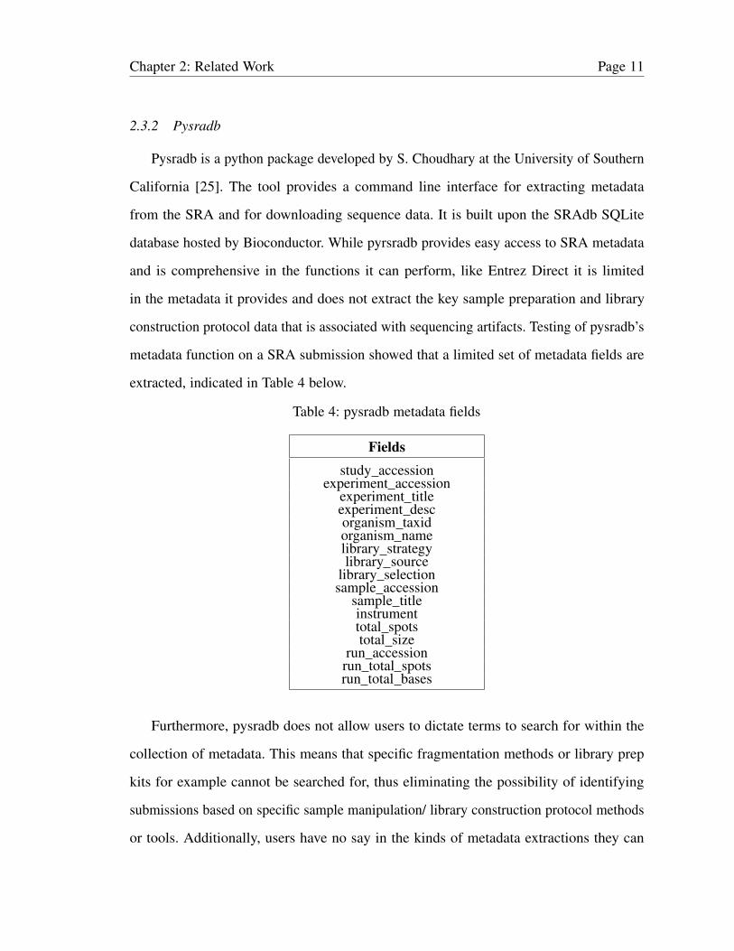
2.3.2 Pysradb

Pysradb is a python package developed by S. Choudhary at the University of Southern

California [25]. The tool provides a command line interface for extracting metadata

from the SRA and for downloading sequence data. It is built upon the SRAdb SQLite

database hosted by Bioconductor. While pyrsradb provides easy access to SRA metadata

and is comprehensive in the functions it can perform, like Entrez Direct it is limited

in the metadata it provides and does not extract the key sample preparation and library

construction protocol data that is associated with sequencing artifacts. Testing of pysradb’s

metadata function on a SRA submission showed that a limited set of metadata fields are

extracted, indicated in Table 4 below.

Table 4: pysradb metadata fields

Fieldsstudy accession

experiment accessionexperiment titleexperiment descorganism taxidorganism namelibrary strategylibrary source

library selectionsample accession

sample titleinstrumenttotal spotstotal size

run accessionrun total spotsrun total bases

Furthermore, pysradb does not allow users to dictate terms to search for within the

collection of metadata. This means that specific fragmentation methods or library prep

kits for example cannot be searched for, thus eliminating the possibility of identifying

submissions based on specific sample manipulation/ library construction protocol methods

or tools. Additionally, users have no say in the kinds of metadata extractions they can

Chapter 2: Related Work Page 12

perform, and are limited to using the provided metadata function. Consequently, a tool

that provides the ability to extract a broader range of metadata fields, enables users to

search for specific terms, and allows users to customize extraction queries, would allow

for more kinds of research to be conducted.

Chapter 3: Materials and Methods Page 13

3 Materials and Methods

In this chapter, the resources used to construct SRAMetadataX for metadata extraction,

the bioinformatics pipeline for identifying artifacts, and the machine learning model

for determining a relationship are described. Details on the processes by which these

components have been developed are also provided.

3.1 SRAMetadataX

SRAMetadataX, short for SRA metadata extractor, is a python program that provides

a command line interface for extracting metadata from the SRA. The tool abstracts the

complexity of querying a database for specific fields and combinations of terms, while

providing a comprehensive set of well documented methods that cover a broad range

of functionality. Most importantly, SRAMetadataX enables extraction of key sample

manipulation and library construction protocol data. SRAMetadataX is available for

download on Github [26].

3.1.1 SRAdb SQlite Package

SRAMetadataX utilizes the curated SRAdb SQLite database hosted by Bioconductor.

SRAdb contains all of the metadata in the SRA, and is continuously updated to include

new submissions [22]. It was developed by J. Zhu and S. Davis of the National Cancer

Institute at the NIH. The data is derived from the SRA XML data that the NCBI makes

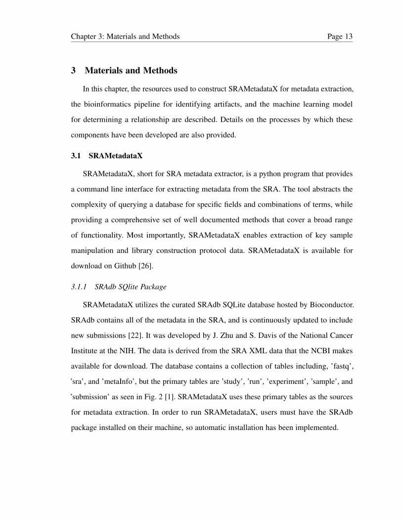
available for download. The database contains a collection of tables including, ’fastq’,

’sra’, and ’metaInfo’, but the primary tables are ’study’, ’run’, ’experiment’, ’sample’, and

’submission’ as seen in Fig. 2 [1]. SRAMetadataX uses these primary tables as the sources

for metadata extraction. In order to run SRAMetadataX, users must have the SRAdb

package installed on their machine, so automatic installation has been implemented.

Chapter 3: Materials and Methods Page 14

Fig. 2: Primary tables of the SRAdb package [1]

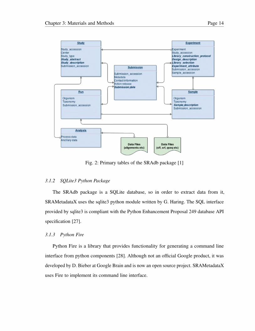
3.1.2 SQLite3 Python Package

The SRAdb package is a SQLite database, so in order to extract data from it,

SRAMetadataX uses the sqlite3 python module written by G. Haring. The SQL interface

provided by sqlite3 is compliant with the Python Enhancement Proposal 249 database API

specification [27].

3.1.3 Python Fire

Python Fire is a library that provides functionality for generating a command line

interface from python components [28]. Although not an official Google product, it was

developed by D. Bieber at Google Brain and is now an open source project. SRAMetadataX

uses Fire to implement its command line interface.

Chapter 3: Materials and Methods Page 15

3.1.4 Methods

SRAMetadataX is comprised of methods that interface with the SRAdb metadata

package, along with auxiliary functions for download and installation. They operate by

constructing and executing SQL queries based on user input to allow for flexibility while

abstracting complexity. The core methods are described in detail in the following sections.

3.1.4.1 init

Upon initialization, SRAMetadataX attempts to connect to the SRAmetadb.sqlite file

provided by the SRAdb package. If it does not find the database in the current directory or

if the user has not previously entered a path to the database, SRAMetadataX prompts the

user to download it or enter a path. After the location of the database has been determined,

whether through download or an entered path, the program connects to the database and

sets the cursor for executing queries. If a path was entered by the user, the path is saved

for future use.

3.1.4.2 download sradb

If the SRAmetadb.sqlite file is not found and the user chooses to download the database

when prompted, this function is called. Alternatively, users are able to call the function

manually at any time, but an error will be raised if the database is found to already exist.

The function first attempts to download the database from an Amazon Web Services S3

bucket; if that download fails, it attempts to download from the NIH. While the file is

downloading, a status bar is provided to indicate progress. Once downloaded, the file is

extracted and a simple query for metadata about the database file is run to verify it works.

3.1.4.3 all sm lcp

This function returns submission accessions for all SRA experiments that contain

sample manipulation/library construction protocol data. Additionally, users can submit

a term or list of terms that submissions also need to contain. For example, a user could

pass the term ”Illumina” to the function so that results are first narrowed down to runs

Chapter 3: Materials and Methods Page 16

sequenced using an Illumina platform. Then, that set of entries is narrowed down to only

ones that contain sample manipulation/library construction protocol data.

3.1.4.4 terms

Terms searches the database for submissions that contain all user provided terms.

It searches the following columns: ’title’, ’study name’, ’design description’, ’sample

name’, ’library strategy’, ’library construction protocol’, ’platform’, ’instrument model’,

’platform parameters’, and ’study abstract’. Essentially, it searches any field that could

possibly contain data linked to the occurrence of sequencing artifacts. Some fields allow

for free-form text entry, so these blocks of text are searched for the occurrence of the

keywords at any point. Users can enter a single term, a list of terms, or the path to a file

containing terms. The function returns run accessions by default, but can also return study

accessions if the user specifies to.

3.1.4.5 keyword match

The keyword match function enables users to extract keywords from metadata based on

a predefined list of terms. Relevant keywords include parameters such as the fragmentation

method, enrichment step, reagents used for DNA extraction, library prep kit, sequencing

platform, and more. It is important that these keywords are extracted accurately and

consistently so they can later be used as features for machine learning analysis. The more

uniform the parameters are between artifacts, the more accurately the model will be able

to elucidate a relationship between the parameters and artifacts. Keyword match ensures

relevant parameters are extracted accurately and uniformly by matching text against a list

of keywords. Users can enter a csv file that dictates keywords per category (fragmentation

methods, reagents, platforms), or use the predefined set provided by SRAMetadataX.

Users are required to provide a list of submissions to perform keyword matching on. This

list can be generated via other functions such as ’all sm lcp’ or ’terms’. Doing so enables

users to narrow down the set of entries to ones that have desired characteristics, such as a

Chapter 3: Materials and Methods Page 17

specific genome. Results are returned in a csv file and saved to a SRAMetadataX specific

”parameters” table in the sqlite database.

3.1.4.6 table info

The table info function returns information about the sqlite database tables. If no

parameter is passed, it returns all tables contained in the database. Users can specify a

table name to get a list of all fields contained within the table.

3.1.4.7 query

The query function allows users who have experience with SQL to enter a custom

query. It provides greater flexibility in situations where none of the provided methods are

able to perform a unique task a user wants. Additionally, the method is used internally by

other functions of SRAMetadataX. Users can access the database scheme easily in order

to construct the query by using the ’table info’ function.

3.1.4.8 srx sa lcp

This function extracts study abstract and/or library construction protocol data for an

SRA experiment or list of experiments. Users can specify the type of data they want to

extract. A sample use case would be to first narrow down entries to ones that contain

sample manipulation/library construction protocol data and a specific term using the

all sm lcp function. Then, results can be passed to srx sa lcp to extract the desired data.

3.2 Bioinformatics Pipeline

In order to identify sequencing artifacts from the SRAMetadataX extracted sequencing

runs, a bioinformatics pipeline was developed. Given a list of run accessions, it produces

a variant calling file containing probable sequencing artifacts for each run. The script can

be executed on a compute cluster and submitted to multiple nodes to be run in parallel.

The file is available on Github and only requires slight modification to paths to be run

on any machine or cluster [26]. An overview of the pipeline is illustrated in Fig. 3 below.

The actions performed and tools used are described in the following sections.

Chapter 3: Materials and Methods Page 18

Fig. 3: Components of the bioinformatics pipeline

3.2.1 Sequence Download and Conversion

The first step of the pipeline is downloading sequencing runs. This action is performed

by using the ’prefetch’ function of the SRA Toolkit. The SRA Toolkit is a collection

of libraries and tools from the NCBI for accessing and converting data housed in the

SRA [29]. The runs are then converted into a usable format called FASTQ, via the

fastq-dump function of the toolkit. FASTQ is a format used for encoding nucleotide

sequences and associated quality scores. It is text-based, with the sequence bases and

quality scores encoded using a single ASCII character [30].

3.2.2 Quality Control

Before proceeding further, the raw sequencing data needs to be evaluated for quality

to identify any problems to be aware of. This is accomplished by using FastQC, a

tool developed by S. Andrews of Babraham Bioinformatics that runs analysis on next

generation sequencing data [31]. Reports are generated that can be viewed in a web

browser.

Chapter 3: Materials and Methods Page 19

3.2.3 Adapter Trimming

Next, adapters are trimmed from sequencing reads. In the process of NGS library

preparation, adapters are ligated to DNA fragments to allow them to attach to the flow cell

lawn for eventual sequencing. Adapter sequences need to be removed from reads because

they can interfere with downstream analyses, including reference genome alignment [32].

Adapter trimming is done using Trimmomatic, a tool developed by A. Bolger et al. that

can handle both single-end and paired-end data [33].

3.2.4 Mapping to Reference Genome

In the process of high throughput sequencing, many short reads are generated that

represent fragments of the original DNA sequence. Thus, the reads need to be mapped

to a reference genome in order to build the full sequence and identify variants. In this

pipeline, mapping is performed by a tool called BWA, short for Burrows-Wheeler Aligner.

BWA maps sequences against large reference genomes, such as the human genome [34].

For this project, the Genome Reference Consortium Human Build 38 (hg38) was used as

the reference genome.

3.2.5 Variant Calling

Next, variant calling is performed. This is the process by which the newly constructed

sequence and the reference genome are compared, and differences are identified. These

differences are the variants, and results are stored in a variant calling file (vcf). Variant

calling is conducted by using bcftools, a set of variant calling utilities that are a part of

the SAMtools suite, written by H. Li [35]. It is important to note that at this point, it

is unknown whether identified variants are naturally occurring mutations or sequencing

artifacts.

3.2.6 Variant Filtering

In the final step of the pipeline, variants are filtered against GIAB high confidence calls.

GIAB has produced browser extensible data (BED) files that contain the chromosome

Chapter 3: Materials and Methods Page 20

coordinates of biologically occuring variants by analyzing data generated from a diverse

set of platforms and methods. A package called BEDTools developed by A. Quinlan

et al. is used to determine the intersection between generated variants and GIAB high

confidence regions, and then bcftools is used to extract only the variants that differ from

the GIAB calls [36]. These variants are likely sequencing artifacts. Generated variants

that do not intersect with the GIAB calls cannot reliably be identified as artifacts, because

they may be biologically occurring variants that have yet to be confidently characterized.

The data undergoes post processing as the last step of the script. This processing includes

converting the vcfs to a tab-delimited format for easier ingestion by the machine learning

pipeline. It is done by using a package called VCFtools hosted on Sourceforge. VCFtools

provides a set of methods for working with variant calling data in vcf file formats [37].

The vcf-to-tab function outputs abnormal column names, so simple bash functions were

used to correct the columns.

3.3 Machine Learning Pipeline

After metadata was extracted from specific sequencing runs using SRAMetadataX

and their artifacts identified via the bioinformatics pipeline, machine learning was applied

to the data to elucidate a relationship between the artifacts and sample manipulation/

library construction protocol parameters. To facilitate model development and enable

reproducibility, the machine learning pipeline was developed in a Jupyter notebook and is

available on Github [26]. The dataset, components of the pipeline, and models developed

are discussed in the following sections.

3.3.1 Data Description

The dataset consists of artifactual variant calls produced by the bioinformatics pipeline

that differ from the GIAB high confidence calls. The variant calling files contain three

columns: chromosome, position, and reference allele/alternate allele. The reference allele

Chapter 3: Materials and Methods Page 21

is the nucleotide/sequence of nucleotides that the GIAB characterized genome contains,

and the alternate allele is that of the sequencing run that differs from the reference.

3.3.2 Data Pre-Processing

The data is imported into a Pandas data frame for use in the machine learning pipeline.

Pandas is a python library developed by W. McKinney for data manipulation [38]. Each

variant calling file is imported separately, and additional columns are added and populated

with user defined numerical values associated with each sample manipulation or library

construction protocol parameter. The three original columns of the variant calling file are

combined into one, because the chromosome, position of the artifact on the chromosome,

and artifact itself together make up one data point. Finally, all data frames are combined

into a single data frame.

3.3.3 Data Evaluation

Before training a model and running prediction, the data is evaluated in order to

determine quality and explore patterns. First, the level of redundancy in the dataset

is examined. Every sequence read run consists of a set of unique artifacts. Between

sequencing runs, there should be a number of repeat artifacts to indicate a pattern that can

be potentially attributed to sample manipulation / library construction protocol variables.

Next, the balance between classes is evaluated. There needs to be as much balance

amongst prediction classes as possible in order to reduce bias towards one prediction over

the other. If there is an imbalance, oversampling can be conducted. Finally, the data is

visualized to further evaluate quality. The n most frequent artifacts found in the dataset are

determined to see if any are a good predictor of the outcome variable, operating under the

assumption that the more frequently an artifact appears, the more likely it has a specific

cause. A histogram is generated to visualize artifact frequencies, and a stacked bar graph

is produced that indicates the proportion of each of the n frequent artifacts that falls

Chapter 3: Materials and Methods Page 22

into each prediction class. All graphs were generated using Matplotlib, a python plotting

library developed by J. Hunter et al. [39]. The data for the experiments conducted for this

project is presented in the results section.

3.3.4 Baseline Model

The machine learning approach that is best suited for elucidating a relationship between

sequencing artifacts and sample manipulation/ library construction protocol parameters

is supervised learning. This is because supervised learning maps an input to an output

based on labeled input-output pairs, and all of the data used for this project is labeled,

whether its the sequencing artifacts or sample/library parameters. Classification and

regression algorithms are supervised learning approaches, and between the two categories

classification is better suited to the problem at hand. Given a sequencing artifact, the

goal is to identify to which of a set of sample manipulation/ library construction protocol

categories the artifact belongs, or in other words classify it. Regression algorithms on the

other hand, seek to predict a continuous outcome variable based on the values of input

variables.

Potential classification algorithms include logistic regression, support vector machines,

k-nearest neighbors, random forest, and more. All of these algorithms were used for

analysis in this project, but for the first experiment conducted logistic regression was used,

and was chosen for its ease of implementation and short training time, and later 10-fold

cross validation showed it to perform as well as all the others. A logistic regression model

predicts discrete values, and is best suited for binary classification. It uses the logistic

function as its transformation function, where the function is seen in Equation 1 and its

sigmoid curve is shown in Fig. 4.

h(x) = 1/(1+ e−x) (1)

Chapter 3: Materials and Methods Page 23

Fig. 4: Standard logistic sigmoid function [3]

The output, h(x), represents probabilities and thus lies within the range of 0 to 1. A

threshold is applied to force calculated probabilities into a binary classification.

For the experiments, the enrichment class of library construction protocol steps was

investigated. Metadata was extracted for sequencing runs that used the NA12878 GIAB

characterized genome and performed either PCR or hybrid capture for target enrichment.

Thus, the two prediction classes for the logistic regression model were PCR and hybrid

capture. The training data was the variant calls, each consisting of the chromosome,

position of the call on the chromosome, reference allele, and variant allele. The variant

calls are categorical data, so they were encoded to transform them into numerical values

recognizable by the logistic regression model. For model training and prediction, the Scikit-

learn library was used. Scikit-learn is a python machine learning library developed by D.

Cournapeau that provides implementations for classification, regression, and clustering

algorithms [40].

3.3.5 Performance Evaluation

To evaluate the performance of the logistic regression model, a confusion matrix was

built using the Scikit-learn metrics package. A confusion matrix depicts the number of

Chapter 3: Materials and Methods Page 24

correct and incorrect predictions divided over the two prediction classes. Additionally, a

classification report was generated to determine precision, recall, and the F1 score.

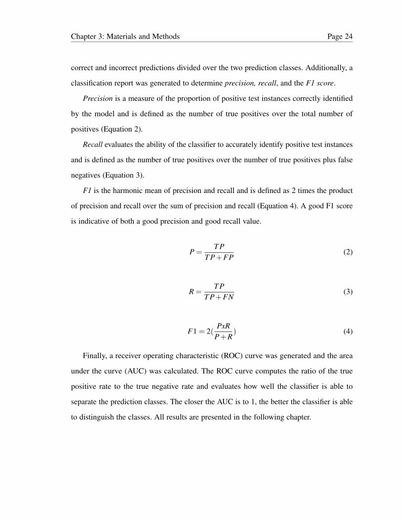
Precision is a measure of the proportion of positive test instances correctly identified

by the model and is defined as the number of true positives over the total number of

positives (Equation 2).

Recall evaluates the ability of the classifier to accurately identify positive test instances

and is defined as the number of true positives over the number of true positives plus false

negatives (Equation 3).

F1 is the harmonic mean of precision and recall and is defined as 2 times the product

of precision and recall over the sum of precision and recall (Equation 4). A good F1 score

is indicative of both a good precision and good recall value.

P =T P

T P+FP(2)

R =T P

T P+FN(3)

F1 = 2(PxR

P+R) (4)

Finally, a receiver operating characteristic (ROC) curve was generated and the area

under the curve (AUC) was calculated. The ROC curve computes the ratio of the true

positive rate to the true negative rate and evaluates how well the classifier is able to

separate the prediction classes. The closer the AUC is to 1, the better the classifier is able

to distinguish the classes. All results are presented in the following chapter.

Chapter 4: Results Page 25

4 Results

In the following sections, results from extracting metadata with SRAMetadataX,

producing artifacts with the bioinformatics pipeline, and applying machine learning are

presented and discussed.

4.1 SRAMetadataX Performance

Every function of SRAMetadataX was thoroughly tested to ensure viability. Sample

output for each core function can be viewed in Appendix B. The tool was able to extract

all relevant metadata fields queried with execution time between 30 seconds and 5 minutes.

Functions such as ’all sm lcp’ and ’terms’ that search the entire SRAdb took the longest

to complete, but that behavior was expected since the SRAdb package is over 30 gigabytes

in size.

The main function used for the experiments conducted was ’terms’. The SRAdb was

searched for submissions matching the terms ’NA12878, hybrid’ and ’NA12878, PCR’.

Fig. 5 shows a snapshot of the results. In Fig. 6, the SRA experiment page for submission

ERR1831349 is displayed with the terms highlighted to validate the accuracy of the

results.

Fig. 5: Partial output of terms function search for NA12878 and hybrid/PCR

Chapter 4: Results Page 26

Fig. 6: Experiment page for run ERR1831349 with ’hybrid’ and ’NA12878’ termshighlighted

Out of each list of run accessions returned, four were chosen for artifact detection and

are listed in Table 5.

Table 5: Chosen SRA run accessions

Hybrid Capture PCRERR1831349 ERR032972ERR1905889 SRR1620964ERR1905890 ERR1679737ERR1831350 ERR032971

4.2 Identifying Artifacts

The pipeline successfully processed the eight chosen sequencing runs and generated

variant calling files consisting of suspected artifacts. Quality control checks using FastQC

Chapter 4: Results Page 27

showed good quality raw sequence data. An example per base sequence quality graph

from the FastQC report is shown in Fig. 7 for run ERR032971. As expected, the quality

of the sequence drops towards the end, likely due to the sequence adapter. Thus, adapter

trimming is performed next using Trimmomatic in order to reduce bias in downstream

analysis.

Fig. 7: FastQC report per base sequence quality graph for run ERR032971

Variant calling files initially included auxiliary fields such as unique identifier, Phred-

scaled quality score, and applied filters. These fields were dropped during conversion to

tab-delimited format. A snapshot of the final variant calling file for ERR032971 consisting

of suspected artifacts is shown in Fig. 8.

Chapter 4: Results Page 28

Fig. 8: Tab-delimited artifacts file for ERR032971 in the final format ingested by themachine learning pipeline

4.3 Application of Machine Learning

4.3.1 Data Pre-Processing

Each tab-delimited artifacts file was imported as a Pandas dataframe, and the associated

hybrid capture/PCR class was added as a binary column ’y’, with hybrid capture labeled as

0 and PCR labeled as 1. The dataframes were concatenated and cleaned up for readability.

An excerpt from the final dataframe is seen in Fig. 9. The total number of artifacts in the

dataset was 298,936.

Fig. 9: Excerpt of dataframe containing all artifacts and associated enrichment procedureclass

Chapter 4: Results Page 29

Thus, the categorical input variable consisted of the chromosome, position, reference

allele, and artifact allele, and the binary predict variable consisted of the target enrichment

procedure- either hybrid capture or PCR.

4.3.2 Data Exploration

The dataset was evaluated for redundancy, and it was found that 192,157 of the

298,936 artifacts are unique- approximately 64%. This means that about 36% of the

dataset consists of artifacts that occur two or more times across various sequencing runs,

indicating that they are less likely chance occurences. Next, the dataset was evaluated for

prediction class balance, and it was found that 151,042 artifacts originated from DNA

enriched through hybrid capture and 147,894 from PCR (Fig. 10). Thus, the classes are

well balanced and oversampling was not required.

Fig. 10: Prediction class balance in the dataset between hybrid capture (HC) and PCR

Finally, the data was evaluated for artifact frequency operating under the hypothesis

that the more frequently an artifact appears, the more likely it has a specific cause. The 20

most frequent artifacts are shown in Fig. 11. The distribution of enrichment procedure

amongst each group of most frequent artifacts is shown in Fig. 12.

Chapter 4: Results Page 30

Fig. 11: Counts of the 20 most frequent artifacts

Fig. 12: Proportion of hybrid capture vs. PCR for each set of most frequent artifacts

Chapter 4: Results Page 31

Based on the results, these artifacts appear to be a decent predictor of enrichment

protocol step. There is a slight bias for hybrid capture among the majority of frequently

occuring artifacts, except in the case of five which are close to a 50% distribution.

4.3.3 Encoding

One-hot encoding was first attempted, but resulted in a kernel crash likely due to

the high cardinality of the artifact feature that required too much memory. Thus, target

encoding was used instead. With target encoding, categorical values are replaced with the

mean of the target variable. The first five artifacts of the dataset and their encoded value

are displayed in Fig. 13.

Fig. 13: Excerpt of artifacts and their target encoding

4.3.4 Model Training and Prediction

The dataset was split into train and test blocks with a ratio of 70% train and 30% test.

Because the data consists of only one feature, the artifacts, it was reshaped so that the

logistic regression model could ingest it. After training, prediction was performed on the

test set with a threshold of 0.5, and an accuracy of 70% was achieved.

4.3.5 Performance Evaluation

The confusion matrix for the prediction is seen in Table 6. It shows that 62,465 correct

predictions were made, and 27,216 incorrect predictions were made.

The classification report is shown in Fig. 14. The average precision score indicates

that when an artifact is predicted to have been produced via PCR, it is correct about 74%

of the time. The average recall score indicates that for all the artifacts actually produced

Chapter 4: Results Page 32

Table 6: Confusion Matrix

n = 89681 Predicted: HC Predicted: PCRActual: HC 21858 23475

Actual: PCR 3741 40607

via PCR, 70% have been correctly identified. The accuracy indicates that of the entire

test set, 70% of the predicted enrichment methods were the enrichment method used to

produce the corresponding artifact.

Fig. 14: Classification report for the prediction

The ROC curve is shown in Fig. 15. The AUC of 0.70 indicates that the model is

able to distinguish between PCR and hybrid capture 70% of the time. It is within the 0.7

- 0.8 range, so not outstanding but acceptable. An AUC of 0.5 corresponds to a model

with no skill that makes purely random predictions. Thus, the results obtained indicate

that the model is able to identify enough of a pattern in the dataset to make non random

predictions.

4.3.6 Experiment 2

In experiment 2, one hot encoding was attempted by reducing the cardinality of the

artifacts feature. The dataset was cut down to the 3000 most frequent unique artifacts

for a total of 15,776 artifacts. Then one hot encoding was performed. Next, recursive

feature elimination (RFE) was conducted in order to reduce the 3000 features to the 20

best performing ones. After applying logistic regression, a slightly increased accuracy of

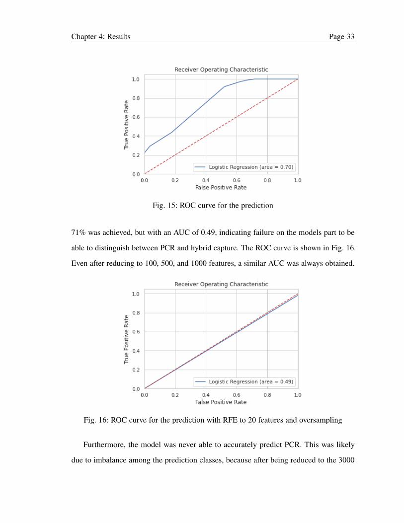
Chapter 4: Results Page 33

Fig. 15: ROC curve for the prediction

71% was achieved, but with an AUC of 0.49, indicating failure on the models part to be

able to distinguish between PCR and hybrid capture. The ROC curve is shown in Fig. 16.

Even after reducing to 100, 500, and 1000 features, a similar AUC was always obtained.

Fig. 16: ROC curve for the prediction with RFE to 20 features and oversampling

Furthermore, the model was never able to accurately predict PCR. This was likely

due to imbalance among the prediction classes, because after being reduced to the 3000

Chapter 4: Results Page 34

most frequent artifacts there was a new imbalance among the prediction classes with

approximately 11500 hybrid capture and 4500 PCR. Thus, oversampling was performed

using the Synthetic Minority Oversampling Technique which at a high level creates

synthetic samples from the minority class by randomly choosing one of the k-nearest

neighbors for a observation and using it to create a similar, but randomly tweaked, new

observation [41]. After oversampling there was a balance of 7933 artifacts for each of

hybrid capture and PCR. Then, RFE was performed to cut the data down to 20 features,

but a lower accuracy of 0.28 was achieved with an AUC of 0.49, and this time no correct

hybrid capture predictions were made. Possibly with more data than just the 3000 most

frequent artifacts the model would have done better, but 3000 was about the maximum the

kernel could take for one hot encoding before crashing. So for the rest of the experiments

target encoding was used.

4.3.7 Experiment 3

In experiment 3, multiple classification models were tested including k-nearest

neighbors, support vector machine, random forest, and multilayer perceptron. For each

model 10-fold cross validation was performed in order to estimate its skill. By doing

cross-validation, an estimate was made for how each model would perform on unseen

data. Results of cross validation showed all models to have an accuracy of 69% +/- 1%

except for the k-nearest neighbors model which achieved an accuracy of 66% +/- 5%. The

AUC of each model saw an improvement over previous experiments, as seen in Fig. 17.

All had an AUC of 0.77 except the k-nearest neighbors model which obtained an AUC of

0.76. These AUCs indicate that the models were able to effectively distinguish between

hybrid capture and PCR.

Chapter 4: Results Page 35

Fig. 17: ROC curves for 10-fold cross-validated models

Chapter 5: Conclusion and Future Work Page 36

5 Conclusion and Future Work

5.1 Conclusion

In this project, a tool called SRAMetadataX has been developed that provides a

command line interface for easy and comprehensive extraction of SRA metadata, including

sample manipulation and library construction protocol steps. The tool was used to identify

sequencing runs that utilized the GIAB characterized NA12878 genome and hybrid capture

or PCR for enrichment. Eight runs were chosen from the set and fed to a bioinformatics

pipeline to identify 298,936 potential sequencing artifacts. Machine learning models were

built and trained on the data to elucidate a relationship between enrichment method and

sequencing artifacts. Review of the results showed that the models were able to predict

enrichment method with about 70% accuracy, indicating that different enrichment methods

likely produce specific sequencing artifacts.

5.2 Future Work

Future work can be done to improve upon SRAMetadataX and the machine learning

application. SRAMetadataX would benefit from a method of quality control to ensure that

the identified experiments that contain desired parameter keywords have actually used the

parameters for their intended purposes. This could be done by reporting the section of

surrounding text for each parameter to the user. Alternatively, natural language processing

(NLP) could be implemented for more advanced verification of intended use. NLP could

also be experimented with as a method for keyword matching.

Further application of machine learning will help to elucidate the relationship between

sample manipulation and library construction protocol steps and the artifacts they cause.

The main objective of this project was to develop a tool that could extract rare metadata

that other existing tools can not. Thus, the application of machine learning in this project

was a proof of concept, and further experimentation with more data would likely result in

Chapter 5: Conclusion and Future Work Page 37

higher accuracy and insight. Additionally, it would be beneficial to conduct an experiment

in which all of the sequencing runs that have a specific artifact are amalgamated, and

machine learning is applied to see if any of the various sample manipulation/library

construction protocol variables seem to be a good predictor of that artifact.

References Page 38

References

[1] J. Alnasir and H. P. Shanahan, “Investigation into the annotation of protocolsequencing steps in the sequence read archive,” GigaSci, vol. 23, 2015.

[2] S. Head, H. Komori, S. Lamere, T. Whisenant, F. Nieuwerburgh, D. Salomon, andP. Ordoukhanian, “Library construction for next-generation sequencing: Overviewsand challenges,” BioTechniques, vol. 56, pp. 61–77, 02 2014.

[3] P.-F. Verhulst, “Notice sur la loi que la population poursuit dans son accroissement,”Correspondance Mathematique et Physique, vol. 3, Dec. 2014.

[4] T. Goetz, “23andme will decode your DNA for $1000. welcome to the age ofgenomics,” Wired, 2007.

[5] NIH, Human Genome Project Completion: Frequently Asked Questions. NationalHuman Genome Research Institute (NHGRI), 2020.

[6] B. Arbeithuber, K. D. Makova, and I. Tiemann-Boege, “Artifactual mutations resultingfrom DNA lesions limit detection levels in ultrasensitive sequencing applications,”DNA Res., vol. 23, no. 6, p. 547–559, 2016.

[7] Y. W. Asmann, M. B. Wallace, and E. A. Thompson, “Transcriptome profiling usingnext-generation sequencing,” Gastro., vol. 135, no. 5, p. 1466–1468, 2008.

[8] M. Costello, T. J. Pugh, and T. J. Fennell, “Discovery and characterization of artifactualmutations in deep coverage targeted capture sequencing data due to oxidative DNAdamage during sample preparation,” Nuc. Acids Res., vol. 41, no. 6, 2013.

[9] M. A. Depristo, E. Banks, and R. Poplin, “A framework for variation discovery andgenotyping using next-generation DNA sequencing data,” ”Nat. Genet., vol. 43, no. 5,p. 491–498, 2011.

[10] S. Behjati and P. S. Tarpey, “What is next generation sequencing?,” Archives ofdisease in childhood. Education and practice edition, vol. 98, no. 6, 2013.

[11] “NGS workflow steps,” 2020. https://www.illumina.com/science/technology/next-generation-sequencing/beginners/ngs-workflow.html.

References Page 39

[12] “Single-nucleotide polymorphism / SNP — Learn Science at Scitable,” 2015. www.nature.com.

[13] N. Tanaka, A. Takahara, T. Hagio, R. Nishiko, J. Kanayama, O. Gotoh, et al.,“Sequencing artifacts derived from a library preparation method using enzymaticfragmentation,” PLoS ONE, vol. 15, no. 1, 2020.

[14] J. Zook, “Genome in a Bottle,” Oct 2020. https://www.nist.gov/programs-projects/genome-bottle.

[15] D. Wheeler, T. Barrett, D. Benson, S. Bryant, K. Canese, et al., “Database resourcesof the National Center for Biotechnology Information,” Nucleic Acids Research,vol. 36, 2008.

[16] “Availability of data and materials : authors and referees @ npg,” 2014. www.nature.com.

[17] L. Chen, P. Liu, T. C. Evans, and L. M. Ettwiller, “DNA damage is a major cause ofsequencing errors, directly confounding variant identification,” Bio., 2016.

[18] X. Ma and J. Zhang, “Analysis of error profiles in deep next-generation sequencingdata,” Molec. and Cell. Bio. / Genet., 2019.

[19] J. M. Zook, D. Catoe, and M. Salit, “Extensive sequencing of seven human genomesto characterize benchmark reference materials,” Scien. Data, vol. 3, no. 1, 2016.

[20] J. M. Zook, B. Chapman, J. Wang, D. Mittelman, O. Hofmann, W. Hide, and M. Salit,“Integrating human sequence data sets provides a resource of benchmark SNP andindel genotype calls,” Nat. Biotech., vol. 32, no. 3, p. 246–251, 2014.

[21] B. Carlson, “Next generation sequencing: The next iteration of personalized medicine:Next generation sequencing along with expanding databases like The Cancer GenomeAtlas, has the potential to aid rational drug discovery and streamline clinical trials,”Biotech. Healthcare, vol. 9, no. 2, 2012.

[22] Y. Zhu, R. Stephens, P. Meltzer, and S. Davis, “SRAdb: query and use publicnext-generation sequencing data from within R,” BMC bioinformatics, vol. 14, no. 1,2013.

References Page 40

[23] N. R. Coordinators, “Database resources of the National Center for BiotechnologyInformation,” Nucleic Acids Research, vol. 41, 2012.

[24] K. J., “Entrez direct: E-utilities on the unix command line,” In: Entrez ProgrammingUtilities Help [Internet]. Bethesda (MD): National Center for BiotechnologyInformation (US) ;, vol. 2010, 2020.

[25] S. Choudhary, “pysradb: A Python package to query next-generation sequencingmetadata and data from NCBI Sequence Read Archive,” F1000Research, vol. 8, Apr.2019.

[26] Z. Tom, “Srametadatax Github Repository,” 2020. https://github.com/ZachPTom/SRAMetadataX.

[27] G. Haring, “sqlite3 DB-API 2.0 interface for sqlite databases,” 2020. https://docs.python.org/3/library/sqlite3.html.

[28] D. Bieber, “Python Fire,” 2018. https://davidbieber.com/projects/python-fire/.

[29] S. Staff, “Using the SRA Toolkit to convert SRA files into other formats,” SRAKnowledge Base, 2011.

[30] P. J. A. . F. Cock, C. J. . Goto, N. . Heuer, M. L. . Rice, and P. M., “The SangerFASTQ file format for sequences with quality scores, and the Solexa/illumina FASTQvariants,” Nucleic Acids Research, vol. 38, no. 6, 2009.

[31] S. Andrews, “FastQC,” 2019. https://www.bioinformatics.babraham.ac.uk/projects/fastqc/.

[32] Illumina, “Adapter Trimming,” 2016. https://support.illumina.com/bulletins/2016/04/adapter-trimming-why-are-adapter-sequences-trimmed-from-only-the--ends-of-reads.html.

[33] A. M. Bolger et al., “Trimmomatic: a flexible trimmer for Illumina sequence data,”Bioinformatics, vol. 30, no. 15, 2014.

[34] H. Li and R. Durbin, “Fast and accurate short read alignment with Burrows-Wheelertransform,” Bioinformatics, vol. 25, no. 14, 2009.

References Page 41

[35] H. Li, B. Handsaker, A. Wysoker, T. Fennell, J. Ruan, et al., “The SequenceAlignment/Map format and SAMtools,” Bioinformatics, vol. 25, no. 16, 2009.

[36] A. Quinlan et al., “bedtools: a powerful toolset for genome arithmetic,” 2009.https://bedtools.readthedocs.io/en/latest/.

[37] P. Danecek, A. Auton, G. Abecasis, C. A. Albers, E. Banks, et al., “The Variant CallFormat and VCFtools,” Bioinformatics, 2011.

[38] W. McKinney, “Python for data analysis,” O’Reilly Media, p. 5, 2017.

[39] J. Hunter, D. Dale, E. Firing, M. Droettboom, et al., “Matplotlib: Visualization withPython,” 2012. https://matplotlib.org/.

[40] F. Pedregosa, G. Varoquaux, A. Gramfort, V. Michel, et al., “Scikit-learn: MachineLearning in Python,” Journal of Machine Learning Research, vol. 12, pp. 2825–2830,2011.

[41] K. W. Bowyer, N. V. Chawla, L. O. Hall, and W. P. Kegelmeyer, “SMOTE: syntheticminority over-sampling technique,” CoRR, vol. abs/1106.1813, 2011.

Appendices Page 42

Appendix A

Sequence Read Archive

A.1 SRA Submission Guidelines

Fig. 18: Guidelines for submitting data and metadata to the SRA.

Appendices Page 43

A.2 SRA Experiment Page

Fig. 19: Sample SRA experiment submission page.

Appendices Page 44

Appendix B

SRAMetadataX Function Output

B.1 download sradb

Fig. 20: SRAdb package download with status bar.

B.2 all sm lcp

Fig. 21: Submissions that used the NA12878 genome, Illumina HiSeq 2000, wholegenome sequencing, and PCR, and contain sm/lcp data.

B.3 query

Fig. 22: Query for metainfo about the SRAdb SQLite database.

B.4 srx sa lcp

B.5 table info

B.6 terms

Appendices Page 45

Fig. 23: Study abstract/library construction protocol data for SRX7949756 andSRX321552.

Fig. 24: Fields of the experiment table.

Fig. 25: Submissions that contain the terms ‘NA12878’ and ‘PCR’.