
bioelec phen
46
63 CHAPTER 3 Bioelectrical Phenomena 3.1 Overview As described in the previous chapter, there is a difference in the composition of electrolytes in the intracellular and extracellular fluids. This separation of charges at the cell membrane and the movement of charges across the membrane are the source of electrical signals in the body. Exchange of ions through ion channels in the membrane is one of the primary signal mechanisms for cell communication and function. For example, normal function in the brain is a matter of the appropriate relay of electrical signals and subsequent neurotransmitter release. Through elec- trical signals, neurons communicate with each other and with organs in the body. Neurons and muscle cells were the first to be recognized as excitable in response to an electrical stimulus. Later, many other cells were found to be excitable in associa- tion with cell motion or extrusion of material from the cells, for example secretion of insulin from the pancreatic beta cells. A few uses of evaluating bioelectrical phe- nomena are summarized in Table 3.1. It is important to understand the conductivity of electricity in the body and time-dependent changes in bioelectrical phenomena. Abnormal electrical activity in the tissue leads to many diseases including that in the heart, brain, skeletal muscles, and retina. Substantial progress in research and clinical practice in electrophysiol- ogy has occurred through the measurement of electrical events. Understanding that the body acts as a conductor of the electrical currents generated by a source such as the heart and spreads within the whole body independently of an electrical source position led to the possibility of placing electrodes on the body surface noninva- sively (i.e., without surgical intervention) to measure electrical potentials. ECG has become a common diagnostic tool to monitor heart activity. Understanding the movement of ions, relating the ion transfer to the function of cells with knowledge about mechanisms of tissues and organ function, and the complex time-dependent changes in electrical signals, and propagation in excitable media is important for development of advanced computational tools and models. This chapter provides an introduction to these concepts.
-
Upload
muhammad-rezal -
Category
Documents
-
view
131 -
download
8
Transcript of bioelec phen

63
C H A P T E R 3
Bioelectrical Phenomena
3.1 Overview
As described in the previous chapter, there is a difference in the composition of electrolytes in the intracellular and extracellular fluids. This separation of charges at the cell membrane and the movement of charges across the membrane are the source of electrical signals in the body. Exchange of ions through ion channels in the membrane is one of the primary signal mechanisms for cell communication and function. For example, normal function in the brain is a matter of the appropriate relay of electrical signals and subsequent neurotransmitter release. Through elec-trical signals, neurons communicate with each other and with organs in the body. Neurons and muscle cells were the first to be recognized as excitable in response to an electrical stimulus. Later, many other cells were found to be excitable in associa-tion with cell motion or extrusion of material from the cells, for example secretion of insulin from the pancreatic beta cells. A few uses of evaluating bioelectrical phe-nomena are summarized in Table 3.1.
It is important to understand the conductivity of electricity in the body and time-dependent changes in bioelectrical phenomena. Abnormal electrical activity in the tissue leads to many diseases including that in the heart, brain, skeletal muscles, and retina. Substantial progress in research and clinical practice in electrophysiol-ogy has occurred through the measurement of electrical events. Understanding that the body acts as a conductor of the electrical currents generated by a source such as the heart and spreads within the whole body independently of an electrical source position led to the possibility of placing electrodes on the body surface noninva-sively (i.e., without surgical intervention) to measure electrical potentials. ECG has become a common diagnostic tool to monitor heart activity. Understanding the movement of ions, relating the ion transfer to the function of cells with knowledge about mechanisms of tissues and organ function, and the complex time-dependent changes in electrical signals, and propagation in excitable media is important for development of advanced computational tools and models. This chapter provides an introduction to these concepts.
Madihally_Book_2.indb 63Madihally_Book_2.indb 63 3/4/2010 5:22:27 PM3/4/2010 5:22:27 PM

64 Bioelectrical Phenomena
3.2 Membrane Potential
The bilayered cell membrane functions as a selectively permeable barrier separat-ing the intracellular and extracellular fluid compartments. The difference in the ion concentration between the intracellular and extracellular compartments creates an electrical potential difference across the membrane, which is essential to cell sur-vival and function. The electrical potential difference between the outside and in-side of a cell across the plasma membrane is called the membrane potential (ΔΦm). The electric potential difference is expressed in units of volts (named after Alessan-dro Volta, an Italian physicist), which is sometimes referred to as the voltage. Under resting conditions, all cells have an internal electrical potential (Φi), usually negative to outside (Φo) (Figure 3.1). This is because of a small excess of negative ions inside the cell and an excess of positive ions outside the cell. Convention is to define the internal electrical potential referenced to the external fluid, which is assumed to be at ground (or zero) potential. When the cell is not generating other electrical signals, the membrane potential is called the resting potential (ΔΦrest) and it is determined by two factors:
Table 3.1 Uses of Bioelectrical Flow Analysis
At the overall body level Body composition and body hydration by measuring electrical characteristics of biological tissue.
Transcutaneous electrical nerve stimulation (TENS), a noninvasive electroanalgesia used in physiotherapy to control both acute and chronic pain arising from several conditions.
At the tissue level Electrocardiogram (ECG or EKG), pacemakers, defibrillators.
Electroencephalogram (EEG): records spontaneous neural activity in the brain and understand brain functions with time and spatial resolution.
Electroneurogram (ENG): records neural activity at the periphery.
Electromyogram (EMG): records activity in the muscle tissue.
Electrogastrogram (EGG): records signals in the muscles of the stomach.
Electroretinogram (ERG): detects retinal disorders.
At the cell level Understanding cellular mechanisms in transport of various molecules, developing novel therapeutic molecules.
Figure 3.1 A part of the membrane of an excitable cell at rest with part of the surrounding intra-cellular and extracellular media. The direction of electrical and diffusional fl uxes is opposing. In the fi gure, the assumption is that cell membrane is permeable to only K+ ions.
Madihally_Book_2.indb 64Madihally_Book_2.indb 64 3/4/2010 5:22:29 PM3/4/2010 5:22:29 PM

3.2 Membrane Potential 65
• Differences in specific ion concentrations between the intracellular and ex-tracellular fluids;
• Differences in the membrane permeabilities for different ions, which is re-lated to the number of open ion channels.
At rest, separation of charges and ionic concentrations across the membrane must be maintained for the resting potential to remain constant. At times, mem-brane potential changes in response to a change in the permeability of the mem-brane. This change in permeability occurs due to a stimulus, which may be in the form of a foreign chemical in the environment, a mechanical stimulus such as shear stress, or electrical pulses. For example, when the axon is stimulated by an electrical current, the Na+ ion channels at that node open and allow the diffusion of Na+ ions into the cell (Figure 3.1). This free diffusion of Na+ ions is driven by the greater concentration of Na+ ion outside the cell than inside (Table 3.2). Ini-tially, diffusion is aided by the electric potential difference across the membrane. As the Na+ ion concentration inside the cell increases, the intracellular potential rises from –70 mV towards zero. A cell is said to be depolarized when the inside becomes more positive and it is said to be hyperpolarized when the inside becomes more negative. At the depolarized state, the Na+ ion diffusion is driven only by the concentration gradient, and continues despite the opposing electric potential dif-ference. When the potential reaches a threshold level (+35 mV), the K+ ion chan-nels open and permit the free diffusion of K+ ions out of the cell, thereby lowering and ultimately reversing the net charge inside the cell. When the K+ ion diffusion brings the intracellular potential back to its original value of resting potential (–70 mV), the diffusion channels close and the Na+ and K+ ion pumps turn on. Na+/K+ ion pumps are used to pump back Na+ and K+ ions in the opposite direction of their gradients to maintain the balance at the expense of energy. The Na+ ion pump transports Na+ ions out of the cell against the concentration gradient and the K pump transports K+ ions into the cell, also against the concentration gradi-ent. When the original K+ ion and Na+ ion imbalances are restored the pumps stop transporting the ions. This entire process is similar in all excitable cells with the variation in the threshold levels.
3.2.1 Nernst Equation
The movement of ions across the cell wall affects the membrane potential. To un-derstand the changes in membrane potential, relating it to the ionic concentration change is necessary. Consider the movement of molecules across the membrane, which is driven by two factors: the concentration gradient and the electrical gradi-ent (Figure 3.1). Analogous to the concentration flux discussed in Chapter 2, (2.8), electrical flux (Jelectric) across a membrane with a potential gradient (dΔΦ), in the x-dimension (dx) is written as
electric
z dJ u C
z dxΔΦ
= − (3.1)
Madihally_Book_2.indb Sec1:65Madihally_Book_2.indb Sec1:65 3/4/2010 5:22:32 PM3/4/2010 5:22:32 PM

66 Bioelectrical Phenomena
where z is the valency on each ion (positive for cations and negative for anions), |z| is the magnitude of the valency, C is the concentration of ions [kgmol/m3], and u is the ionic mobility [m2/V.s]. Ionic mobility is the velocity attained by an ion moving through a gas under a unit electric field (discussed in Section 3.4.1), similar to the diffusivity constant described in (2.8). Ionic mobility is related to the diffusivity constant by
ABD z Fu
RT= (3.2)
where F is the Faraday’s constant, which is equal to the charge on an electron (in Coulombs), times the number of ions per mole given by the Avogadro’s number (6.023 × 10²³). Substituting (3.2) into (3.1),
ABelectric
zFD dJ C
RT dx
− ΔΦ= (3.3)
In (3.3), product zFC is the amount of charge per unit volume or charge density [C/m3]. The total flux is given by the sum of electrical fluxes and the diffusional fluxes (3.8).
ABtotal AB
zFDdC dJ D C
dx RT dxΔΦ
= − − (3.4)
Equation (3.4) is known as the Nernst-Planck equation and describes the flux of the ion under the combined influence of the concentration gradient and an elec-tric field. At equilibrium conditions, Jtotal is zero. Hence, (3.4) reduces to
ABAB
zFDdC dD C
dx RT dxΔΦ
= − (3.5)
Rearranging (3.5), and integrating between the limits ΔΦ = ΔΦi when C = Ci and ΔΦ = ΔΦo when C = Co gives
ΔΦ = Φ − Φ = −[mM][J/mol.K] [K]
[V] ln[C/mol] [mM]
irest i o
o
CR TzF C
(3.6)
Equation (3.6) is called the Nernst equation (named after the German physi-cal chemist Walther H. Nernst) and is used to calculate a potential for every ion in the cell knowing the concentration gradient. The subscript i refers to the inside of the cell and the subscript o refers to the outside. In addition, the ratio RT/zF is the ratio of thermal energy to electrical energy. RT/F is 26.71 mV at 37°C. Converting
Madihally_Book_2.indb Sec1:66Madihally_Book_2.indb Sec1:66 3/4/2010 5:22:34 PM3/4/2010 5:22:34 PM

3.2 Membrane Potential 67
natural logarithm to logarithm of base 10, the constant is 61.5 mV at 37°C or 58 mV at 25°C.
EXAMPLE 3.1
What is the resting ΔΦ for Na+ ions, if the outside concentration is 140 mM and the inside concentration is 50 mM?
50ln 26.17ln 26.95 mV
140i
i oNao
RT CzF C
+ΔΦ = Φ − Φ = − = − =
3.2.2 Donnan Equilibrium
Both sides of the cell membrane have two electrolyte solutions and the cell mem-brane is selectively permeable to some ions but blocks the passage of many ions. Thus, one charged component is physically restricted to one phase. This restriction can also result from the inherently immobile nature of one charged component, such as fixed proteins. In either case, an uneven distribution of the diffusible ions over the two phases develops, as their concentrations adjust to make their electro-chemical potentials the same in each phase. In turn, this establishes an osmotic pres-sure difference and an electric potential difference between the phases. This type of ionic equilibrium is termed a Donnan equilibrium, named after Irish physical chemist Frederick G. Donnan. According to the Donnan equilibrium principle, the product of the concentrations of diffusible ions on one side of the membrane equals that product of the concentration of the diffusible ions on the other side. Number of cations in any given volume must be equal to number of anions in the same volume (i.e., space charge neutrality—outside of a cell, net charge should be zero). In other words, to maintain equilibrium, an anion must cross in the same direction for each cation crossing the membrane in one direction, or vice versa. Assuming that a mem-brane is permeable to both K+ and Cl− but not to a large cation or anion (Figure 3.2), the Nernst potentials for both K+ and Cl− must be equal at equilibrium, that is,
, ,
,0 ,0
ln lnK i Cl i
K Cl
C CRT RTF C F C
− =
or
=,0 ,
, ,0
K Cl i
K i Cl
C C
C C (3.7)
Madihally_Book_2.indb Sec1:67Madihally_Book_2.indb Sec1:67 3/4/2010 5:22:37 PM3/4/2010 5:22:37 PM

68 Bioelectrical Phenomena
Equation (3.7) is a Donnan equilibrium. The rule is important because it con-tributes to the origin of resting potential. In general, when the cell membrane is at rest, the active and passive ion flows are balanced and a permanent potential exists across a membrane only if the membrane is impermeable to some ion(s) and an active pump is present. The Donnan equilibrium only applies to situations where ions are passively distributed (i.e., there are no metabolic pumps utilizing energy regulating ion concentration gradients across the membrane).
EXAMPLE 3.2
A cell contains 100 mM of KCl and 500 mM of protein chloride. The outside of the cell medium has 400 mM KCl. Assuming that the cell membrane is permeable to Cl− and K+ ions and impermeable to the protein, determine the equilibrium concentrations and the membrane potential. Also assume that these compounds can completely dissociate.
,0 , ,0 , ,0 ,0500, 1,000, and K K j Cl Cl i K ClC C C C C C+ = + = =
From (3.7) we have K,0 Cl,0
K,0 Cl,0
1,000
500 C C
C C−=
−
or
,0 ,0 , ,333 mM, 167 mM, and 667 mMK Cl K i Cl iC C C C= = = =
Also,
33326.71ln 18.4 mV
167K ClΦ = Φ = =
The Donnan equilibrium is useful in pH control in red blood cells (RBCs). When RBCs pass through capillaries in the tissue, CO2 released from tissues and water diffuse freely into the red blood cells. They are converted to carbonic acid, which dissociates into hydrogen and bicarbonate ions, as described in Section 3.2.4. H+ ions do not pass through cell membranes but CO2 passes readily. This situation cannot be sustained as the osmolarity and cell size will rise with intracellular H+ and bicarbonate ion concentration, and rupture the cell. To circumvent this situa-tion, the bicarbonate ion diffuses out to the plasma in exchange for Cl− ions due to
Figure 3.2 Space charge neutrality.
Madihally_Book_2.indb Sec1:68Madihally_Book_2.indb Sec1:68 3/4/2010 5:22:39 PM3/4/2010 5:22:39 PM

3.2 Membrane Potential 69
the Donnan equilibrium. The discovery of this chloride shift phenomenon is attrib-uted to Hamburger HJ, which is popularly called Hamburger’s chloride shift. An ion exchange transporter protein in the cell membrane facilitates the chloride shift. A build up of H+ ions in the red blood cell would also prevent further conversion and production of the bicarbonate ion. However, H+ ions bind easily to reduced hemoglobin, which is made available when oxygen is released. Hence, free H+ ions are removed from the solution. Reduced hemoglobin is less acidic than oxygenated hemoglobin. As a result of the shift of Cl− ions into the red cell and the buffering of H+ ions onto reduced hemoglobin, the intercellular osmolarity increases slightly and water enters causing the cell to swell. The reverse process occurs when the red blood cells pass through the lung.
3.2.3 Goldman Equation
Most biological components contain many types of ions including negatively charged proteins. However, the Nernst equation is derived for one ion after all per-meable ions are in Donnan equilibrium. The membrane potential experimentally measured is often different than the Nernst potential for any given cell, due to the existence of other ions. An improved model is called the Goldman equation (also called the Goldman-Hodgkin-Katz equation), named after American scientist Da-vid E. Goldman, which quantitatively describes the relationship between membrane potential and permeable ions. According to the Goldman equation, the membrane potential is a compromise between various equilibrium potentials, each dependent on the membrane permeability and absolute ion concentration. Assuming a planar and infinite membrane of thickness (L) with a constant membrane potential (ΔΦm),
mddx L
ΔΦΦ= (3.8)
Substituting (3.8) into (3.4) and rearranging gives
total m
AB
dCdx
J z FC
D RTL
−=
ΔΦ+
(3.9)
Equation (3.9) is integrated across the membrane with the assumption that total flux is constant and C = Ci when x = 0, C = Co when x = L. Furthermore, con-sidering the solubility of the component using (3.14), and rearranging an equation to the total flux is obtained as:
ln
1
m
m
zF
RTmem m i o
total zF
RT
P zF C C eJ
RTe
ΔΦ⎛ ⎞−⎜ ⎟⎝ ⎠
ΔΦ⎛ ⎞−⎜ ⎟⎝ ⎠
⎡ ⎤− ΔΦ −⎢ ⎥= ⎢ ⎥
⎢ ⎥−⎣ ⎦
(3.10)
Madihally_Book_2.indb Sec1:69Madihally_Book_2.indb Sec1:69 3/4/2010 5:22:42 PM3/4/2010 5:22:42 PM

70 Bioelectrical Phenomena
For multiple ions, the ion flux through the membrane at the resting state is zero. For example, consider the three major ions involved in the nerve cell stimula-tion, Na+, K+, and Cl− ions. Then,
total K Na ClJ J J J+ + −= + +
Rewriting (3.10) for each molecule and simplification provides
+ + −
+ + −
⎛ ⎞+ +ΔΦ = ΔΦ − ΔΦ = − ⎜ ⎟+ +⎝ ⎠
[K ] [Na ] [Cl ]ln
[K ] [Na ] [Cl ]K i Na i Cl o
m i oK o Na o Cl i
P P PRTF P P P (3.11)
where PNa, PK, and PCl are the membrane permeabilities of Na+, K+, and Cl ions, respectively. If only one ion is involved then (3.11) reduces to (3.7).
EXAMPLE 3.3
A mammalian cell present in an extracellular fluid similar to Figure 3.2. The intracellu-lar fluid composition is also similar to Figure 3.2. If the cell is permeable to Cl−, K+, and Na+ ions with a permeability ratio of 0.45: 1.0: 0.04, what is the resting potential of the membrane? From (3.11)
50ln 26.17ln 26.95 mV
140i
i oNao
RT CzF C
+ΔΦ = Φ − Φ = − = − =
[Na ] = 10 mM+
[K ] = 140 mM+
[Cl ] = 4 mM−
[Na ] = 142 mM+
[K ] = 4 mM+
[Cl ] = 103 mM−
3.3 Electrical Equivalent Circuit
3.3.1 Cell Membrane Conductance
The flow of ions through the cell membrane is controlled by channels and pumps. Hence, the rate of flow of ions depends on the membrane permeability or conduc-tance (G) to a species in addition to the driving force (i.e., membrane potential difference). Rate of flow of ions (or rate of charge of charge) is called the current and Ampere is a unit in SI units. The relationship between current I, potential dif-ference, and conductance is written as
I G= ΔΦ (3.12)
Madihally_Book_2.indb Sec1:70Madihally_Book_2.indb Sec1:70 3/4/2010 5:22:44 PM3/4/2010 5:22:44 PM

3.3 Electrical Equivalent Circuit 71
where G is the conductance (siemens, S = A/V) of the circuit and ΔΦ is the mem-brane potential (i.e., the voltage between inside and outside of the cell membrane). Equation (3.12) is called Ohm’s law. The reciprocal of conductance is called resis-tance and a widely used form of Ohm’s law in electrical engineering is:
IR
ΔΦ= (3.13)
where R is the resistance. All substances have resistance to the flow of an electric current. For example, metal conductors such as copper have low resistance whereas insulators have very high resistances. Pure electrical resistance is the same when ap-plying direct current and alternating current at any frequency. In the body, highly conductive (or low resistance electrical pathway) lean tissues contain large amounts of water and conducting electrolytes. Fat and bone, on the other hand, are poor conductors with low amounts of fluid and conducting electrolytes. These changes form the basis of measuring the body composition in a person.
When the cell membrane is “at rest,” it is in the state of dynamic equilibrium where a current leak from the outside to inside is balanced by the current provided by pumps and ion channels so that the net current is zero. In this dynamic equilib-rium state, ionic current flowing through an ion channel is written as
= ΔΦ − Δ ,( ( ) )i m rest iI G t φ (3.14)
Δφrest,i is the equilibrium potential for the ith species, and Δφ m(t) − Δφrest,i is the net driving force.
EXAMPLE 3.4
If a muscle membrane has a single Na+ ion channel conductance of 20 pS, find the cur-rent flowing through the channel when the membrane potential is −30 mV. The Nernst potential for the membrane is +100 mV.
( )( )
( ) ( ) ( )( )12 3 3 1220 10 30 10 100 10 2.6 10 2.6 pA
m restI g t
S V V A− − − −
= ΔΦ − ΔΦ
= × − × − × = − × = −
3.3.2 Cell Membrane as a Capacitor
Intracellular and extracellular fluids are conducting electrolytes, but the lipid bi-layer is electrically nonconductive. Thus the nonconductive layer is sandwiched be-tween two conductive compartments. It can be treated as a capacitor consisting of two conducting plates separated by an insulator or nonconductive material known
Madihally_Book_2.indb Sec1:71Madihally_Book_2.indb Sec1:71 3/4/2010 5:22:47 PM3/4/2010 5:22:47 PM

72 Bioelectrical Phenomena
as a dielectric. Hence, the cell membrane is modeled as a capacitor, charged by the imbalance of several different ion species between the inside and outside of a cell. A dielectric material has the effect of increasing the capacitance of a vacuum-filled parallel plate capacitor when it is inserted between its plates. The factor K by which the capacitance is increased is called the dielectric constant of that material. K varies from material to material, as summarized in Table 3.1 for few materials.
Consider the simplest dielectric-filled parallel plate capacitor whose plates are of cross sectional area A and are spaced a distance d apart. The formula for the membrane capacitance, Cm, of a dielectric-filled parallel plate capacitor is
=m
AC
dε (3.15)
where e (= Kε0) is called the permittivity of the dielectric material between the plates. The permittivity ε of a dielectric material is always greater than the permittivity of a vacuum e0. Thus, from (3.15), Cm increases with the dielectric constant surface area (space to store charge) and decreases with an increase in membrane thickness. The cell membrane is modeled as a parallel plate capacitor, with the capacitance proportional to the membrane area. Hence, measuring the membrane capacitance allows a direct detection of changes in the membrane area occurring during cellular processes such as exocytosis and endocytosis (discussed in Chapter 2). The spacing between the capacitor plates is the thickness of the lipid double layer, estimated to be 5 to 10 nm. Capacitors store charge of electrons for a period of time depending on the resistance of the dielectric. The amount of charge, Qch, a capacitor holds is determined by
= ΔΦch mQ C (3.16)
The unit of capacitance is called a farad (F), equivalent to coulombs per volt. The typical value of capacitance for biological membranes is approximately 1 mF/cm2. For a spherical cell with the diameter of 50 mm, the surface area is 7.854 × 10⁻⁵ cm2. Then the total capacitance is 12.73 μF. The amount of reactants is proportional to the charge and available energy of capacitor (described in Section 3.4.1). The number of moles of ions that move across the membranes is calculated using the relation
=chQ nzF (3.17)
where n is the number of moles of charge separated.
Table 3.1 Dielectric Constant of a Few Materials
Material Vacuum Air Water Paper Pyrex Membrane Teflon
K 1 1.00059 80 3.5 4.5 2 2.1
Madihally_Book_2.indb Sec1:72Madihally_Book_2.indb Sec1:72 3/4/2010 5:22:49 PM3/4/2010 5:22:49 PM

3.3 Electrical Equivalent Circuit 73
EXAMPLE 3.4
If a cell membrane has a capacitance of 0.95 mF/cm2, how many K+ ions need to cross the membrane to obtain a potential of 100 mV? From (3.16),
20.95 * 0.1 0.095 /cmch mQ C Cμ= ΔΦ = =
From (3.17),
μ
−×= = =
+×
6 22
23
0.095 10 ( /cm )5,930 ions per m of membrane
96,484( 1) * /ions
6.023 10
chQ Cn
zF C
Capacitors oppose changes in voltage by drawing or supplying current as they charge or discharge to the new voltage level. In other words, capacitors conduct current (rate of change of charge) in proportion to the rate of voltage change. The current that flows across a capacitor is
0
1 tch m
C m m cm
dQ dI C i dt
dt dt C
ΔΦ= = ΔΦ = ∫ (3.18)
Ionic current described by (3.12) is different than capacitative current. In a circuit containing a capacitor with a battery of ΔΦrest [Figure 3.3(a)], the capacitor charges linearly until the voltage reaches a new steady state voltage, ΔΦSS [Figure 3.3(b)]. After reaching the new voltage, the driving force is lost. Since the volt-age does not change, there is no capacitative current flow. The capacitance of the membrane per unit length determines the amount of charge required to achieve a certain potential and affects the time needed to reach the threshold. In other words, slop of the line in Figure 3.3(b) is affected by capacitance. When the conductance is increased by two, steady state voltage is reduced. However, the slope of the line is much higher.
Capacitive reactance (RC) (generally referred to as reactance and expressed in ohms, Ω) is the opposition to the instantaneous flow of electric current caused by
Figure 3.3 (a, b) Circuit with a capacitor.
Madihally_Book_2.indb Sec1:73Madihally_Book_2.indb Sec1:73 3/4/2010 5:22:51 PM3/4/2010 5:22:51 PM

74 Bioelectrical Phenomena
capacitance. Reactances pass more current for faster-changing voltages (as they charge and discharge to the same voltage peaks in less time), and less current for slower-changing voltages. In other words, reactance for any capacitor is inverse-ly proportional to the frequency of the alternating current. In alternating current (AC) circuit, reactance is expressed by
1
2Cm
RfCπ
= (3.19)
where f is the frequency of the alternating current in hertz. Equation (3.19) suggests that reactance is the reciprocal of frequency (i.e., reactance decreases as frequency increases). At very low frequencies reactance is nearly infinite. However, capaci-tance is independent of frequency and indirectly defines cell membrane volume. Ideally reactance is expressed in capacitance at a given frequency. Large capacitance values mean a slower rate of ion transfer.
3.3.3 Resistance-Capacitance Circuit
Based on the above discussion, the cell membrane has both resistive and capacita-tive properties. Then, a cell membrane can be represented by an equivalent circuit of a single resistor and capacitor in parallel (Figure 3.4) with a resting potential calculated using the Nernst equation for an individual ionic species. When mul-tiple ionic species are involved in causing changes in electrical activity, resistance of each species is considered separately. It is conceived that cells and their supporting mechanisms are not a series of extracellular and intracellular components but reside in parallel with a small series effect from the nucleolus of the cells. Simplification of circuits with resistors in series or parallel by replacing them with equivalent resistors is possible using the Kirchoff’s laws in electrical circuits. Two resistors in series are replaced by one whose resistance equals the sum of the original two resis-tances, since voltage and resistance are proportional. Reciprocals of resistances of two resistors in parallel are added to obtain the equivalent resistance since current and resistance are inversely proportional. Conversely, capacitor values are added normally when connected in parallel, but are added in reciprocal when connected in series, exactly the opposite of resistors.
Figure 3.4 Equivalent circuit of a cell wall.
Madihally_Book_2.indb Sec1:74Madihally_Book_2.indb Sec1:74 3/4/2010 5:22:53 PM3/4/2010 5:22:53 PM

3.3 Electrical Equivalent Circuit 75
To describe the behavior of an RC circuit, consider K+ ion conductance in series with its Nernst potential (ΔΦrest). A positive stimulus current, Iinj, is injected from time t0 to t. Then using Kirchoff’s current rule, the equivalent circuit of a cell is written as
0C i injI I I+ − =
where IC is current through the capacitor and Ii is the ionic current through the resistor. The injected current is subtracted from the other two. This is based on the convention that the current is positive when positive charge flows out of the cell membrane. Substituting (3.14) and (3.18),
0m restmm inj
m
dC I
dt R
ΔΦ − ΔΦΔΦ+ − = (3.20)
Due to injected current, the membrane reaches a new state potential, ΔΦSS. At steady state d ΔΦm/dt = 0, (3.20) reduces to
SS inj m restI RΔΦ = + ΔΦ
Rearranging and integrating with the limits ΔΦ = ΔΦo when Δt = Δto and ΔΦ = ΔΦ when Δt = Δt
( )( )
0 0ln SS
SS
t t
τ
ΔΦ − ΔΦ −=
ΔΦ − ΔΦ
where τ is the product of Rm and Cm and has the units of time. In generally, τ is called the time constant. An alternative form is
( )0
0
t t
SS SS e τ
−⎛ ⎞⎜ ⎟⎝ ⎠ΔΦ = ΔΦ + ΔΦ − ΔΦ (3.21)
Equation (3.21) is used for both charging and discharging of an RC circuit for any ionic species. In general, the majority of experiments are conducted by inject-ing a current as a step input to understand the property of a cellular membrane with respect to a particular ionic species. A frequently measured property is τ to understand the resistance and capacitance properties of cells. At the instant when the current is first turned on (t = 0) the first term in square brackets ΔΦSS is zero and ΔΦ = ΔΦrest. For t >> 0, the second term is nearly zero and ΔΦ = ΔΦSS.
Madihally_Book_2.indb Sec1:75Madihally_Book_2.indb Sec1:75 3/4/2010 5:22:55 PM3/4/2010 5:22:55 PM
76 Bioelectrical Phenomena
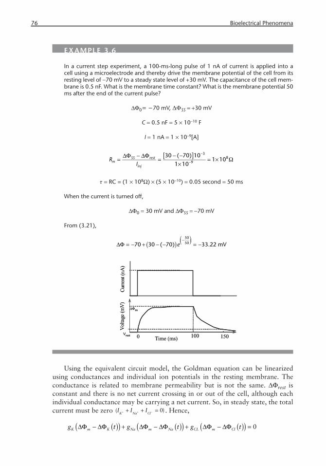
EXAMPLE 3.6
In a current step experiment, a 100-ms-long pulse of 1 nA of current is applied into a cell using a microelectrode and thereby drive the membrane potential of the cell from its resting level of −70 mV to a steady state level of +30 mV. The capacitance of the cell mem-brane is 0.5 nF. What is the membrane time constant? What is the membrane potential 50 ms after the end of the current pulse?
ΔΦ0= −70 mV, ΔΦSS = +30 mV
C = 0.5 nF = 5 × 10⁻¹⁰ F
I = 1 nA = 1 × 10⁻⁹[A]
[ ] −
−− −ΔΦ − ΔΦ
= = = × Ω×
38
9
30 ( 70) 101 10
1 10SS rest
minj
RI
τ = RC = (1 × 10⁸Ω) × (5 × 10⁻¹⁰) = 0.05 second = 50 ms
When the current is turned off,
ΔΦ0 = 30 mV and ΔΦSS = −70 mV
From (3.21),
( )⎛ ⎞−⎜ ⎟⎝ ⎠ΔΦ = − + − − = −
505070 30 ( 70) 33.22 mVe
Time (ms)
Volt
age
(mV
)C
urr
ent
(nA
)
0 100 150
ΔΦss
Vrest
Time (ms)
Volt
age
(mV
)C
urr
ent
(nA
)
0 100 150
ΔΦss
Vrest
Using the equivalent circuit model, the Goldman equation can be linearized using conductances and individual ion potentials in the resting membrane. The conductance is related to membrane permeability but is not the same. ΔΦrest is constant and there is no net current crossing in or out of the cell, although each individual conductance may be carrying a net current. So, in steady state, the total current must be zero ( 0)
K Na ClI I I+ + −+ + = . Hence,
( )( ) ( )( ) ( )( ) 0K m K Na m Na CL m Clg t g t g tΔΦ − ΔΦ + ΔΦ − ΔΦ + ΔΦ − ΔΦ =
Madihally_Book_2.indb Sec1:76Madihally_Book_2.indb Sec1:76 3/4/2010 5:22:58 PM3/4/2010 5:22:58 PM

3.3 Electrical Equivalent Circuit 77
Solving for the membrane potential,
K K Na Na Cl Clm
K Na Cl
g g g
g g g
ΔΦ + ΔΦ + ΔΦΔΦ =
+ + (3.22)
Since K+, Na+, and Cl− ions are not at their equilibrium potentials, (3.22) gives a steady state potential and not an equilibrium state potential. There is a continuous flux of those ions at the resting membrane potential. Often the equilibrium poten-tial is not computed explicitly but defined as an independent leakage potential ΔΦL and determined by the resting potential. If the sum of current across the membrane is not zero, then charge builds up on one side of the membrane while changing the potential. Then, measuring the current flowing across a cell helps in determining the capacitative and the resistive properties if the membrane potential is known. Conductance properties of two ionic species can also be obtained in terms of the membrane potentials. Consider a cell with a transfer of K+ ions and Na+ ions. Then
( )( ) ( )( ) 0K m K Na m Nag t g tΔΦ − ΔΦ + ΔΦ − ΔΦ =
Rearranging this gives
( )
( )m KNa
K m Na
g
g
− ΔΦ − ΔΦ=
ΔΦ − ΔΦ (3.23)
Thus, in steady-state, the conductance ratio of the ions is equal to the inverse ratio of the driving forces for each ion.
EXAMPLE 3.7
Electrical activity of a neuron in culture was recorded with intracellular electrodes. The ex-periments were carried out at 37°C. The normal saline bathing the cell contained 145-mM Na+ ions and 5.6-mM K+ ions. In this normal saline, the membrane potential was measured to be −46 mV, but if the Na was replaced with an impermeant ion (i.e., the cell was bathed in a Na-free solution) the membrane potential increased to −60 mV. In the normal saline the ENa was +35 mV, so that the membrane is impermeable to Cl−. To simplify the issue you can ignore Na efflux in the Na-free saline condition. What ratio of gNa to gK would account for the normal membrane potential? From (3.23),
( )( )− − −
= =− − +46 ( 60)
0.1746 ( 35)
Na
K
gg
Madihally_Book_2.indb Sec1:77Madihally_Book_2.indb Sec1:77 3/4/2010 5:23:01 PM3/4/2010 5:23:01 PM

78 Bioelectrical Phenomena
3.3.4 Action Potential
The transport of ions causes cells to change their polarization state. Many times a small depolarization may not create a stimulus. Typically, cells are characterized by threshold behavior (i.e., if the signal is below the threshold level, no action is observed). The intensity of the stimulus must be above a certain threshold to trigger an action. The smallest current adequate to initiate activation of a cell is called the rheobasic current or rheobase. The threshold level can be reached either by a very high strength signal for a short duration or a low strength signal applied for a long duration. The membrane potential may reach the threshold level by a short, strong stimulus or a longer, weaker stimulus. Theoretically, the rheobasic current needs an infinite duration to trigger activation. The time needed to excite the cell with twice rheobase current is called chronaxy. If the membrane potential is given a suf-ficiently large constant stimulus, the cell is made to signal a response. This localized change in polarization, which is later reset to the original polarization, is called an action potential [Figure 3.5(a)]. This large local change in polarization triggers the same reaction in the neighborhood, which allows the reaction to propagate along the cell.
The transfer of Na+ and K+ ions across the membrane are primarily responsi-ble for the functioning of a neuron. When the neuron is in a resting state, the cell membrane permeabilities are very small as many of the Na+ and K+ ion channels are closed; the cell interior is negatively charged (at −70 mV) relative to the exte-rior. When a stimulus is applied that depolarizes a cell, the cell surface becomes
Figure 3.5 Action potential: (a) characteristics features of an action potential curve; (b) changes in charge distribution during depolarization; (c) Hodgkin-Huxley equivalent circuit for a squid axon; and (d) voltage clamp measurement circuit.
Madihally_Book_2.indb Sec1:78Madihally_Book_2.indb Sec1:78 3/4/2010 5:23:03 PM3/4/2010 5:23:03 PM
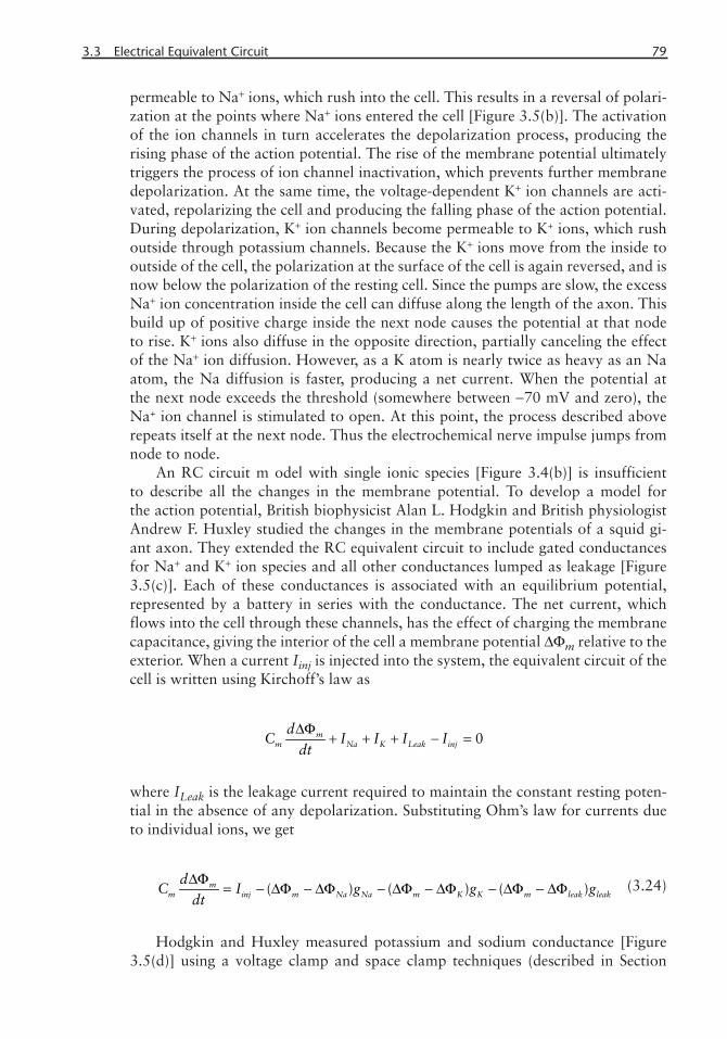
3.3 Electrical Equivalent Circuit 79
permeable to Na+ ions, which rush into the cell. This results in a reversal of polari-zation at the points where Na+ ions entered the cell [Figure 3.5(b)]. The activation of the ion channels in turn accelerates the depolarization process, producing the rising phase of the action potential. The rise of the membrane potential ultimately triggers the process of ion channel inactivation, which prevents further membrane depolarization. At the same time, the voltage-dependent K+ ion channels are acti-vated, repolarizing the cell and producing the falling phase of the action potential. During depolarization, K+ ion channels become permeable to K+ ions, which rush outside through potassium channels. Because the K+ ions move from the inside to outside of the cell, the polarization at the surface of the cell is again reversed, and is now below the polarization of the resting cell. Since the pumps are slow, the excess Na+ ion concentration inside the cell can diffuse along the length of the axon. This build up of positive charge inside the next node causes the potential at that node to rise. K+ ions also diffuse in the opposite direction, partially canceling the effect of the Na+ ion diffusion. However, as a K atom is nearly twice as heavy as an Na atom, the Na diffusion is faster, producing a net current. When the potential at the next node exceeds the threshold (somewhere between −70 mV and zero), the Na+ ion channel is stimulated to open. At this point, the process described above repeats itself at the next node. Thus the electrochemical nerve impulse jumps from node to node.
An RC circuit m odel with single ionic species [Figure 3.4(b)] is insufficient to describe all the changes in the membrane potential. To develop a model for the action potential, British biophysicist Alan L. Hodgkin and British physiologist Andrew F. Huxley studied the changes in the membrane potentials of a squid gi-ant axon. They extended the RC equivalent circuit to include gated conductances for Na+ and K+ ion species and all other conductances lumped as leakage [Figure 3.5(c)]. Each of these conductances is associated with an equilibrium potential, represented by a battery in series with the conductance. The net current, which flows into the cell through these channels, has the effect of charging the membrane capacitance, giving the interior of the cell a membrane potential ΔΦm relative to the exterior. When a current Iinj is injected into the system, the equivalent circuit of the cell is written using Kirchoff’s law as
0mm Na K Leak inj
dC I I I I
dt
ΔΦ+ + + − =
where ILeak is the leakage current required to maintain the constant resting poten-tial in the absence of any depolarization. Substituting Ohm’s law for currents due to individual ions, we get
( ) ( ) ( )mm inj m Na Na m K K m leak leak
dC I g g g
dt
ΔΦ= − ΔΦ − ΔΦ − ΔΦ − ΔΦ − ΔΦ − ΔΦ (3.24)
Hodgkin and Huxley measured potassium and sodium conductance [Figure 3.5(d)] using a voltage clamp and space clamp techniques (described in Section
Madihally_Book_2.indb Sec1:79Madihally_Book_2.indb Sec1:79 3/4/2010 5:23:05 PM3/4/2010 5:23:05 PM

80 Bioelectrical Phenomena
3.3.4) and empirically fitted curves to the experimental data. They modeled the time dependency on the ionic conductance by a channel variable or activation coef-ficients, which indicate the probability of a channel being open. In general, the con-ductance for a time-dependent channel is written in terms of the channel variable (x), ranging from zero to one, and the maximum conductance. They developed a set of four differential equations to demonstrate action potential of the membrane. There are sophisticated programs, which allow simulating various action poten-tials. Whenever a short (millisecond range) inward current pulse (in the nano-am-pere range) is applied to a patch of axonal membrane, the membrane capacitance is charged and the membrane potential depolarizes. As a result n and m are increased. If the current pulse is sufficient in strength then the generated INa will exceed IK, resulting in a positive feedback loop between activation m and INa. Since tm is very small at these potentials, the sodium current shifts the membrane potential beyond 0 mV. As sodium inactivation h and IK increase, the membrane potential returns to its resting potential and even undershoots a little due to the persistent potas-sium current. If Iinj = 0, it can be proved that the rest state is linearly stable but it is excitable if the perturbation from the steady state is sufficiently large. For Iinj = 0 there is a range where repetitive firing occurs. Both types of phenomena have been observed experimentally in the giant axon of the squid. Hodgkin and Huxley per-formed their voltage clamp experiments at 6.3°C. Higher temperatures affect the reversal potentials since the Nernst equation is temperature dependent. Tempera-ture affects the transition states of ion channels dramatically. Higher temperatures lead to lower time constants and decreased amplitudes. A multiplication factor for each time constant has been developed to account for temperature. Although the Hodgkin-Huxley model is too complicated to analyze, it has been extended and applied to a wide variety of excitable cells. There are experimental results in both skeletal muscle and cardiac muscle, which indicate that a considerable fraction of the membrane capacitance is not “pure,” but has a significant resistance in series with it. This leads to modifications in the electrical equivalent circuit of the mem-brane. Understanding the behavior of ion channels has also allowed simplification of the model. One such is the Fitzhugh-Nagumo model, based on the time scales of the Na+ and K+ ion channels. The Na+ channel works on a much faster time scale than the K+ channel. This fact led Fitzhugh and Nagumo to assume that the Na+
channel is always in equilibrium, which allowed them to reduce the four equations of the Hodgkin and Huxley model to two equations.
3.3.5 Intracellular Recording of Bioelectricity
Measurements of membrane potential, both steady-state and dynamic changes, have become key to understanding the activation and regulation of cellular re-sponses. Developing mathematical models that depict physiological processes at the cellular level depends on the ability to measure required data accurately. One has to measure or record the voltage and/or current across the membrane of a cell, which requires access to inside the cell membrane. Typically, the tip of a sharp microelectrode (discussed in Section 3.5) is inserted inside the cell. Since such mea-surements involve low-level voltages (in the millivolts range) and have high source resistances, usage of amplifiers is an important part of bioinstrumentation signals
Madihally_Book_2.indb Sec1:80Madihally_Book_2.indb Sec1:80 3/4/2010 5:23:08 PM3/4/2010 5:23:08 PM

3.3 Electrical Equivalent Circuit 81
[Figure 3.5(d)]. Amplifiers are required to increase signal strength while maintain-ing high fidelity. Although there are many types of electronic amplifiers for different applications, operational amplifiers (normally referred to as op-amps), are the most widely used devices. They are called operational amplifiers because they are used to perform arithmetic operations (addition, subtraction, multiplication) with signals. Op-amps are also used to integrate (calculate the areas under) and differentiate (calculate the slopes of) signals. An op-amp is a DC-coupled high-gain electronic voltage amplifier with differential inputs (usually two inputs) and, usually, a single output. Gain is the term used for the amount of increased signal level (i.e., the out-put level divided by the input level). In its ordinary usage, the output of the op-amp is controlled by negative feedback, which almost completely determines the output voltage for any given input due to amplifier’s high gain. Modern designs of op-amps are electronically more rugged and normally implemented as integrated circuits. For complete discussion about op-amps, the reader should refer to textbooks related to electrical circuits.
One technique to measure electrical activity across a cell membrane is the space clamp technique, where a long thin electrode is inserted into the axon (just like in-serting a wire into a tube). Injected current is uniformly distributed over the inves-tigated space of the cell. After exciting the cell by a stimulus, the whole membrane participates in one membrane action potential, which is different from the propa-gating action potentials observed physiologically, but describes the phenomenon in sufficient detail. However, cells without a long axon cannot be space-clamped with an internal longitudinal electrode, and some spatial and temporal nonuniformity exists.
Alternatively, the membrane potential is clamped (or set) to a specific value by inserting an electrode into the axon and applying a sufficient current to it. This is called the voltage clamp technique, the experimental set up used by Hodgkin and Huxley [Figure 3.6(d)]. Since the voltage is fixed, (3.24) simplifies to
( ) ( ) ( )2 2 0inj m N N m K K m leak leakI V g V g V g− ΔΦ − − ΔΦ − − ΔΦ − =
American biophysicist Kenneth S. Cole in the 1940s developed the voltage clamp technique using two fine wires twisted around an insulating rod. This meth-od measures the membrane potential with a microelectrode (discussed in Chapter
Figure 3.6 Electric fi eld: (a) convention of direction; (b) infl uence of point source; and (c) multiple point charges.
Madihally_Book_2.indb Sec1:81Madihally_Book_2.indb Sec1:81 3/4/2010 5:23:10 PM3/4/2010 5:23:10 PM

82 Bioelectrical Phenomena
9) placed inside the cell, and electronically compares this voltage to the voltage to be maintained (called the command voltage). The clamp circuitry then passes a current back into the cell though another intracellular electrode. This electronic feedback circuit holds the membrane potential at the desired level, even when the permeability changes that would normally alter the membrane potential (such as those generated during the action potential). There are different versions of voltage clamp experiments. Most importantly, the voltage clamp allows the separation of membrane ionic and capacitative currents. Therefore, the voltage clamp technique indicates how membrane potential influences ionic current flow across the mem-brane with each individual ionic current. Also, it is much easier to obtain informa-tion about channel behavior using currents measured from an area of membrane with a uniform, controlled voltage, than when the voltage is changing freely with time and between different regions of membrane. This is especially so as the open-ing and closing (gating) of most ion channels is affected by the membrane potential. The voltage clamp method is widely used to study ionic currents in neurons and other cells. However, the errors in the voltage clamp experiment are due to the current flowing across the voltage-clamped membrane, which generates a drop in the resistance potential in series with the membrane, and thus causes an error in control of the potential. This error, which may be significant, can only be partially corrected by electronic compensation. All microelectrodes act as capacitors as well as resistors and are nonlinear in behavior. Subsequent correction by computation is difficult for membrane potentials for which the conductance parameters are volt-age dependent.
A recent version of voltage-clamp experiment is the patch clamp technique. This method has a resolution high enough to measure electrical currents flow-ing through single ion channels, which are in the range of pico-amperes (10−12 A). Patch-clamp refers to the technique of using a blunt pipette to isolate a patch of membrane. The patch-clamp technique was developed by German biophysicist Erwin Neher and German physiologist Bert Sakmann to be able to study the ion currents through single ion channels. The principle of the patch-clamp technique is that a small patch of a cell membrane is electrically isolated by the thin tip of a glass pipette (0.5–1 μm-diameter), which is pressed towards the membrane surface. By application of a small negative pressure, a very tight seal between the membrane and the pipette is obtained. The resistance between the two surfaces is in the range of 109 ohms (G ohm, which is then called the giga-seal). Most techniques for moni-toring whole-cell membrane capacitance work by applying a voltage stimulus via a patch pipette and measuring the resulting currents. Because of the tightness of this seal, different recording configurations can be made.
Patch-clamp technique measurements reveal that each channel is either fully open or fully closed (i.e., facilitated diffusion through a single channel is all or none). Although the initial methods applied a voltage step (similar to Problem 3.7) and analyzed the exponential current decay in the time domain, the most popular methods use sinusoidal voltage stimulation. Patch-clamp technique is also used to study exocytosis and endocytosis from single cells. Nevertheless, cell-attached and excised-patch methods suffer from uncertainty in the area of the membrane patch, which is also likely to be variable from patch to patch, even with consistent pipette geometry. The number of ion channels per patch is another source of variability,
Madihally_Book_2.indb Sec1:82Madihally_Book_2.indb Sec1:82 3/4/2010 5:23:12 PM3/4/2010 5:23:12 PM

3.4 Volume Conductors 83
in particular for channels that are present at low density. There is also a concern that patch formation and excision may alter channel properties. Thus, conductance density estimates obtained from patches are not very reliable.
Another way to observe the electrical activity of a cell is through impedance measurements, which are measured after applying an alternating current. Imped-ance (Z) is a quantity relating voltage to current, and is dependent on both the capacitative and resistive qualities of the membrane. The units of impedance are ohms. In the series pathway, two or more resistors and capacitors are equal to im-pedance as the vector sum of their individual resistance and reactance.
2 2 2cZ R R= + (3.25)
In the parallel pathway, two or more resistors and capacitors are equal to im-pedance as the vector sum of their individual reciprocal resistances and reactance.
2 2 2
1 1 1
cZ R R= + (3.26)
Impedance is also dependent on the frequency of the applied current. For in-stance, if a stimulus is applied, the cell is affected if the impedance measurement changes. A small amplitude AC signal is imposed across a pair of electrodes onto which cells are deposited and the impedance of the system measured. By measuring the current and voltage across a small empty electrode, the impedance, resistance, and capacitance can be calculated. When cells cover the electrode, the measured impedance changes because the cell membranes block the current flow. From the impedance changes, several important properties of the cell layer can be deter-mined such as barrier function, cell membrane capacitance, morphology changes, cell motility, electrode coverage, and how close the cells are to the surface.
Quantitative high-resolution imaging methods show great promise, but present formidable challenges to the experimentalist, and probably cannot be used to ex-tract kinetic data. Immunogold methods can only provide relative densities of spe-cific channel subunits; determining the absolute densities of the channels, and their functional properties require complementary, independent methods.
3.4 Volume Conductors
So far, only time-dependent variations and concentration-dependent variations in bioelectrical activity were discussed with the assumption that the same membrane potential is distributed independent of the location of the source. However, the stimulus propagates in a direction and location becomes an important factor. All biological resistances, capacitances, and batteries are not discrete elements but dis-tributed in a conducting medium of electrolytes and tissues, which continuously extend throughout the body in 3D. Hence they are referred to as volume conduc-tors. For example, electrical activity of the brain spreads (spatially) over the entire head volume. The head is a volume conductor with the conductive brain inside the
Madihally_Book_2.indb Sec1:83Madihally_Book_2.indb Sec1:83 3/4/2010 5:23:14 PM3/4/2010 5:23:14 PM

84 Bioelectrical Phenomena
skull, with another thin conductor on the outside, the skin. Thus, it is modeled with an equivalent source (e.g., a single current dipole) in a specific volume conductor.
3.4.1 Electric Field
A fundamental principle which must be understood in order to grasp volume con-ductors is the concept of the electric field. Every charged object is surrounded by a field where its influence can be experienced. An electrical field is similar to a gravitational field that exists around the Earth and exerts gravitational influences upon all masses located in the space surrounding it. Thus, a charged object creates an electric field, an alteration of the space or field in the region that surrounds it. Other charges in the electrical field would feel the unusual alteration of the space. The electric field is a vector quantity whose direction is defined, by convention, as the direction that a positive test charge would be pushed in when placed in the field. Thus, the electric field direction about a positive source charge is always directed away from the source, and the electric field direction about a negative source charge is always directed toward the source [Figure 3.6(a)].
A charged object can have an attractive effect upon an oppositely charged ob-ject or a repulsive effect upon the same charged object even when they are not in contact. This phenomenon is explained by the electric force acting over the dis-tance separating the two objects. Consider the electric field created by a positively charged (Q) sphere [Figure 3.6(b)]. If another positive charge Q1 enters the electri-cal field of Q, a repulsive force is experienced by that charge. According to Cou-lomb’s law, the amount of electric force is dependent upon the amount of charge and the distance from the source (or the location within the electrical field). The electric force (FE) acting on a point charge Qch as a result of the presence of a sec-ond point charge Q1 is given by
12
C chE
k Q QF
r= (3.27)
where kC is the Coulomb’s law proportionality constant. The units on kC are such that when substituted into the equation the units on charge (coulombs) and the units on distance (meters) will be canceled, leaving a Newton as the unit of force. The value of kC is dependent upon the medium that the charged objects are im-mersed in. For air, kC is approximately 9 × 10⁹ Nm2/C2. For water, kC reduces by as much as a factor of 80. kC is also related to permittivity (ε0) of the medium by the
relation 0
14Ck
πε= and normally Coulomb’s law with permittivity is used.
If two objects of different charges, with one being twice the charge of the other, are moved the same distance into the electric field, then the object with twice the charge requires twice the force. The charge that is used to measure the electric field strength is referred to as a test charge since it is used to test the field strength. The magnitude of the electric field or electrical field strength E is defined as the force per charge of the test charge.
Madihally_Book_2.indb Sec1:84Madihally_Book_2.indb Sec1:84 3/4/2010 5:23:16 PM3/4/2010 5:23:16 PM

3.4 Volume Conductors 85
12 2
0 01
1 14 4
ch chQ Q QFE
q Q r rπε πε= = = (3.28)
The electric field strength in a given region is also referred by the electrical flux, similar to molar flux. Electrical flux is the number of electrical field lines per unit area. The electric field from any number of point charges is obtained from a vec-tor sum of the individual fields [Figure 3.6(c)]. A positive charge is taken to be an outward field and negative charge to be an inward field.
Work is defined as the component of force in the direction of motion of an object times the magnitude of the displacement of the object
gW F d⊥=
For example, if a box is moving in the horizontal direction across the floor, the work done by the force F is Fcosθ (Figure 5.2) times the magnitude of the displace-ment traveled, d, across the floor. Work done by gravitation force is independent of the path and the work done by that force is written as the negative of a change in potential energy, that is,
( )g f iW PE PE= − −
where PEf is the final potential energy and PEi is the initial potential energy. In the gravitational field, objects naturally move from high potential energy to low po-tential energy under the influence of the field force. On the other hand, work must be done by an external force to move an object from low potential energy to high potential energy. Similarly, to move a charge in an electric field against its natural direction of motion would require work. The exertion of work by an external force would in turn add potential energy to the object. Work done by electrical force can also be written, similar to gravitational field, as
( )E f iW PE PE= − −
The work done by the electric force when an object Q1 is moved from point a to point b in a constant electric field is given by
1 cosEW Q E dθ=
where d is the distance between the final position and the initial position, and cosq is the angle between the electric field and the direction of motion. This work would change the potential energy by an amount which is equal to the amount of work done. Thus, the electric potential energy is dependent upon the amount of charge on the object experiencing the field and upon the location within the field.
Madihally_Book_2.indb Sec1:85Madihally_Book_2.indb Sec1:85 3/4/2010 5:23:18 PM3/4/2010 5:23:18 PM

86 Bioelectrical Phenomena
EXAMPLE 3.8
A positive point charge 20C creates an electric field with a strength 4 N/C in the air, when measured at a distance of 9 cm away. What is the magnitude of the electric field strength at a distance of 3 cm away? If a second 3C positive charge, located at 9 cm from the initial first, is moved 4 cm at an angle of 30° to the electrical field, what is the work done on that charge? From (3.38),
= = =1 2 2 21
4[N/C]9 [cm]
C ch C chk Q k QE
d (E3.1)
At location 2,
2 2 23 [cm]
C chk QE = (E3.2)
Dividing (E3.2) by (E3.1),
[ ]
2 2
2 2 2
4[N/C]9 [cm]36 N/C
3 [cm]3[ ] 4[N/C] cos30 0.04[m] 0.415JE
E
W C
= =
= × × × =
An electric dipole is when two charges of the same magnitude and opposite sign are placed relatively close to each other. Dipoles are characterized by their dipole moment, a vector quantity with a magnitude equal to the product of the charge of one of the poles and the distance separating the two poles. When placed in an electric field, equal but opposite forces arise on each side of the dipole creat-ing a torque (or rotational force, discussed in Section 5.2.2), Tele:
eleT pE=
for an electric dipole moment p (in coulomb-meters). Understanding the changes in the direction of the dipole is one of the most important parts of the electrocardio-gram (see Section 3.4.5).
3.4.2 Electrical Potential Energy
While electric potential energy has a dependency upon the charge of the object ex-periencing the electric field, electric potential is purely location dependent. Electric potential is the amount of electric potential energy per unit of charge that would be possessed by a charged object if placed within an electric field at a given location. The electric potential difference (ΔΦ) is the difference in electric potential between the final and the initial location when work is done upon a charge to change its po-tential energy. The work to move a small amount of charge dQch from the negative side to the positive side is equal to ΔΦdQch. As a result of this change in potential
Madihally_Book_2.indb Sec1:86Madihally_Book_2.indb Sec1:86 3/4/2010 5:23:20 PM3/4/2010 5:23:20 PM

3.4 Volume Conductors 87
energy, there is also a difference in electric potential between two locations. In the equation form, the electric potential difference is
E
ch
dW
dQΔΦ =
ΔΦ is determined by the nature of the reactants and electrolytes, not by the size of the cell or amounts of material in it. As the charge builds up in the charging process, each successive element of charge dQch requires more work to force it onto the positive plate. In other words, charge and potential difference are interdepend-ent. Summing these continuously changing quantities requires an integral.
0
chQ
E chW dQ= ΔΦ∫ (3.29)
Substituting (3.16) into the above equation and integrating gives
or2
212 2
Ch mE E
m
Q CW W
C= = ΔΦ (3.30)
The only place a parallel plate capacitor could store energy is in the electric field generated between the plates. This insight allows energy (rather the energy density) calculation of an electric field. The electric field between the plates is ap-proximately uniform and of magnitude, E, which is s/e0, where σ(= QCh/A) is the surface charge density in C/cm2. The electric field elsewhere is approximately zero. The potential difference between the plates is
EdΔΦ = (3.31)
where d is the distance between the plates. The energy stored in the capacitor is written as
2
2 0
2 2m
E
AE dCW
ε= ΔΦ = (3.32)
Ad is the volume of the field-filled region between the plates, so if the energy is stored in the electric field then the energy per unit volume, or energy density, of the field is given by
2
0
2E
EWw
Ad
ε= = (3.33)
Madihally_Book_2.indb Sec1:87Madihally_Book_2.indb Sec1:87 3/4/2010 5:23:22 PM3/4/2010 5:23:22 PM

88 Bioelectrical Phenomena
This equation is used to calculate the energy content of any electric field by dividing space into finite cubes (or elements). Equation (3.43) is applied to find the energy content of each cube, and then summed to obtain the total energy. One
can demonstrate that the energy density in a dielectric medium is 2
2E
Ew
ε= where
ε(= Kε0) is the permittivity of the medium. This energy density consists of two ele-
ments: the energy density 2
0
2Eε held in the electric field, and the energy density
20( 1)
2K Eε− held in the dielectric medium. The density represents the work done on
the constituent molecules of the dielectric in order to polarize them.
EXAMPLE 3.9
Defibrillators are devices that deliver electrical shocks to the heart in order to convert rapid irregular rhythms of the upper and lower heart chambers to normal rhythm. In order to rapidly deliver electrical shocks to the heart, a defibrillator charges a capacitor by apply-ing a voltage across it, and then the capacitor discharges through the electrodes attached to the chest of the patient undergoing ventricular fibrillation. In a defibrillator design, a 64-μF capacitor is charged by bringing the potential difference across the terminals of the capacitor to 2,500V. (a) How much energy is stored in the capacitor?(b) How much charge is then stored on the capacitor? What is the average electrical current (in amperes) that flows through the patient’s body if the entire stored charge is discharged in 10 ms? (c) Using (3.32), the energy stored in the capacitor
( )( )−= × × =26 31
64 10 2.5 10 200J2EW
(d) Charge stored is
( )( )− −= ΔΦ = × × = ×6 3 364 10 2.5 10 400 10ch mQ C C
Alternatively Qch can also be calculated using (3.27)
Average electrical current = −
−×
= =×
3
3
400 1040A
10 10chQ C
time s
3.4.3 Conservation of Charge
Differences in potential within the brain, heart, and other tissues reflect the segre-gation of electrical charges at certain locations within 3D conductors as nerves are excited, causing cell membrane potentials to change. While the potential measured at some distance from an electrical charge generally decreases with increasing dis-tance, the situation is more complex within the body. For example, generators of
Madihally_Book_2.indb Sec1:88Madihally_Book_2.indb Sec1:88 3/4/2010 5:23:24 PM3/4/2010 5:23:24 PM

3.4 Volume Conductors 89
the EEG are not simple point-like charge accumulations but rather are dipole-like layers. Moreover, these layers are convoluted and enmeshed in a volume conductor with spatially heterogeneous conductivity. The particular geometry and orientation of these layers determines the potential distribution within or at the surface of the 3D body. Nevertheless, charged conductors, which have reached electrostatic equi-librium [Figure 3.7(a)] follow these characteristics:
1. The charge spreads itself out when a conductor is charged. 2. The excess charge lies only at the surface of the conductor. 3. Charge accumulates, and the field is strongest on pointy parts of the
conductor. 4. The electric field at the surface of the conductor is perpendicular to the
surface. 5. The electric fi eld is zero within the solid part of the conductor.
Gauss’ law of electricity (named after Carl F. Gauss, a German physicist) is a form of one of Maxwell’s equations, the four fundamental equations for electricity and magnetism. According to Gauss’ law of electricity, for any closed surface that surrounds a volume distribution of charge, the electric flux passing through that surface is equivalent to the total enclosed charge. In other words, if E is the electric field strength [Figure 3.7(b)] and Q is the total enclosed charge, then
0S
QE dA
ε• =∫ (3.34)
where dA is the area of a differential square on the closed surface S with an outward direction facing normal to the surface. ε0, the permittivity of free space is 8.8542 × 10⁻¹² C2/Nm2. The dot product is used to get the scalar part of E as the direction is known to be perpendicular to the area. To prove the Gauss theorem, imagine a sphere with a charge in the center. Substituting for E from (3.38) and denoting dA in spherical coordinates, for ease of use:
Figure 3.7 (a, b) Volume conductors.
Madihally_Book_2.indb Sec1:89Madihally_Book_2.indb Sec1:89 3/4/2010 5:23:26 PM3/4/2010 5:23:26 PM

90 Bioelectrical Phenomena
22
00
. sin4S
Q Qr d d
rθ θ φ
επε=∫
In other words, the area integral of the electric field over any closed surface is equal to the net charge enclosed in the surface divided by the permittivity of space. Gauss’ law is useful for calculating the electrical fields when they originate from charge distributions of sufficient symmetry to apply it. Gauss’ law permits the evaluation of the electric field in many situations by forming a symmetric Gaussian surface surrounding a charge distribution and evaluating the electric flux through that surface. Since charge is enclosed in a 3D space, a normal practice is to express charge either by unit surface area called surface charge density (σch with units C/cm2) or by unit volume basis called charge density (ρch with units C/cm3) and then integrate accordingly. When charge enclosed is electric charge density of ρch, then total charge,
chVQ dVρ= •∫ (3.35)
EXAMPLE 3.10
Consider an infinitely long plate with surface charge density of 2 C/m2 in a medium that has a permittivity of 25 × 10−12 C2/Nm2. What is the electrical field strength? Because the plate is infinite and symmetrical, the only direction the E field can go is perpendicular to the plate. So,
[ ]2 2
2
C/cm * cm 2
S
ch ch
E dA A E
Q A A Cσ
=
⎡ ⎤ ⎡ ⎤= =⎣ ⎦ ⎣ ⎦
∫
From (3.44),
2 chA E Aσ
ε=
Hence
2
12 2 2
2 C/cm
2 2 25 10 [C /Nm ]chE
σ
ε −
⎡ ⎤⎣ ⎦= =× ×
and
ˆ2
chE nσ
ε=
where n̂ is a unit vector perpendicular to the plate.
Madihally_Book_2.indb Sec1:90Madihally_Book_2.indb Sec1:90 3/4/2010 5:23:29 PM3/4/2010 5:23:29 PM

3.4 Volume Conductors 91
The integral form of Gauss’ law finds application in calculating electric fields around charged objects. However, Gauss’s law in the differential form (i.e., diver-gence of the vector electric field) is more useful. If E is a function of space variables x, y, and z in Cartesian coordinates [Figure 3.7(b)], then
E E E
E u v wx y z
∂ ∂ ∂∇ • = + +
∂ ∂ ∂ (3.36)
where u is the unit vector in the x direction, v is the unit vector in the y direction, and w is the unit vector in the z direction. The divergence theorem is used to convert surface integral into a volume integral and the Gauss law is
( )0S V
QE dA E dV
ε• = ∇ • =∫ ∫ (3.37)
Substituting (3.45) for Qch and simplification results in the differential form of Gauss law
0
chEρ
ε∇ • = (3.48)
Since cross production of the electric field is zero ∇ × =( 0)E , E is represented as a gradient of electrical potential, that is,
E = −∇ΔΦ
A negative sign is used based on the convention that electric field direction is away from the positive charge source. Then the divergence of the gradient of the scalar function is
2
0
chρ
ε
−∇ ΔΦ = (3.39)
or
2 2 2
2 2 20
ch
x y z
ρ
ε
−∂ ΔΦ ∂ ΔΦ ∂ ΔΦ+ + =
∂ ∂ ∂ (3.40)
In a region of space where there is no unpaired charge density (ρch = 0), (3.39) reduces to (∇2ΔΦ = 0) Laplace’s equation.
While the area integral of the electric field gives a measure of the net charge en-closed, the divergence of the electric field gives a measure of the density of sources.
Madihally_Book_2.indb Sec1:91Madihally_Book_2.indb Sec1:91 3/4/2010 5:23:31 PM3/4/2010 5:23:31 PM

92 Bioelectrical Phenomena
It also has implications for the conservation of charge. The charge density is ρch on the top plate, and −ρch on the bottom plate. Gauss’s law is always true, but not al-ways useful as a certain amount of surface symmetry is required to use it effectively. In developing EMG, the volume conductor comprises planar muscle and subcuta-neous tissue layers. The muscle tissue is homogeneous and anisotropic while the subcutaneous layer is inhomogeneous and isotropic. However, differential form of Gauss’s law is useful to derive conservation of charge.
According to conservation of charge, the total electric charge of an isolated system remains constant regardless of changes within the system. If some charge is moving through the boundary (rate of change of charge is current), then it must be equal to the change in charge in that volume. To obtain a mathematical ex-pression, consider a gross region of interest called control volume (see Chapter 4) with a charge density ρch. The rate of change of charge across the control surface is grouped as a change in current density Js inside a homogeneous finite volume conductor. A charge density is a vector quantity whose magnitude is the ratio of the magnitude of current flowing in a conductor to the cross-sectional area per-pendicular to the current flow, and whose direction points in the direction of the current. For a simple case of one inlet and one outlet without generation of charge and consumption of charge, the charge-conservation is written as
chin out
dQQ Q
dt= − (3.41)
where Qin is the rate of flow of net charge into the system and Qout is the charge out of the system. However, for biological applications, obtaining an expression for 3D space is necessary. For this purpose, the law of local conservation of charge is obtained using the divergence theorem.
chdJ
dt
ρ= ∇ • (3.42)
Equation (3.42) is called the continuity equation of charge, stating how charge is conserved locally. If the charge density increases in some region locally (yielding a nonzero ∂ρ/∂τ), then this is caused by current flowing into the local region by the amount ∂ρ/∂τ = −∇ • J. If the charge decreases in a local region (a negative −∂ρ/∂τ), then this is due to current flowing out of that region by the amount − ∂ρ/∂τ = −∇ • J. The divergence is taken as a positive corresponding to J spreading outwards. Cur-rent density is related to electric field by J = γE, where γ is the electrical conductivity of a material to conduct an electric current. Then
( ) ( )2
2 ch
J E E
J
γ γ γ
ρ
ε γ
∇ • = ∇ • = ∇ • = − ∇ ΔΦ
∇ •∇ ΔΦ = − =
(3.43)
Madihally_Book_2.indb Sec1:92Madihally_Book_2.indb Sec1:92 3/4/2010 5:23:33 PM3/4/2010 5:23:33 PM

3.4 Volume Conductors 93
Equation (3.43) is popularly called the Poisson equation. The Poisson equation describes the electrical field distribution through a volume conductor, and is the equation utilized in analyzing electrical activity of various tissues. It is solved using many computational tools by two approaches: surface-based and volume-based. In both cases, the volume conductor is divided into small homogeneous finite ele-ments. Finite elements are assumed to be isotropic for surface-based analysis (also referred as the boundary-element method), and integral form of the equation is used. For volume-based analysis, finite elements are anisotopic and a typically dif-ferential form of equations is used.
Knowing the number, location, orientation, and strength of the electrical charge sources inside the head, one could calculate the reading at an electrode on the sur-face of the scalp with Poisson’s equation. However, the reverse is not true (i.e., the estimation of the electrical charge sources using the scalp potential measurements). This is called the inverse problem and it does not have an unique solution. Hence, it is difficult to determine which part of the brain is active by measuring a number of electrical potential recordings at the scalp.
3.4.4 Measuring the Electrical Activity of Tissues: Example of the Electrocardiogram
The fundamental principles of measuring bioelectrical activity are the same for all tissues or cells: the mapping in time and space of the surface electric potential cor-responding to electric activity of the organ. However, for diagnostic monitoring, electrical activity should be measured with less invasiveness, unlike intracellular measurements (described in Section 3.3.5). For this purpose, the concept of volume conduction is used (i.e., bioelectrical phenomena spread within the whole body independent of electrical source position). As the action potential spreads across the body, it is viewed at any instant as an electric dipole (depolarized part being negative while the polarized part is positive). For example, electrical activity of the heart is approximated by a dipole with time varying amplitude and orientation. An electrode placed on the skin measures the change in potential produced by this ad-vancing dipole, assuming that potentials generated by the heart appear throughout the body. This forms the basis of the electrocardiogram (ECG), a simple noninva-sive recording of the electrical activity generated by the heart.
In muscle cells, an active transport mechanism maintains an excess of Na+ and Ca2+ ions on the outside, and an excess of Cl− ions inside. In the heart, resting potential is typically −70 mV for atrial cells and −90 mV for ventricular cells. The positive and negative charge differences across each part of the membrane causes a dipole moment pointing across the membrane from the inside to the outside of the cell. However, each of these individual dipole moments are exactly cancelled by a dipole moment across the membrane on the other side of the cell. Hence, the total dipole moment of the cell is zero. In other words, the resting cell has no dipole moment.
If a potential of 70 mV is applied to the outside of the cell at the left hand side, the membranes’ active transport breaks down at that position of the cell, and the ions rush across the membrane to achieve equilibrium values. The sinoatrial (S-A) node, natural pacemaker of the heart) sends an electrical impulse that starts the
Madihally_Book_2.indb Sec1:93Madihally_Book_2.indb Sec1:93 3/4/2010 5:23:35 PM3/4/2010 5:23:35 PM

94 Bioelectrical Phenomena
wave of depolarization [Figure 3.8(a)]. The equilibrium values turn out to be a slight excess of positive ions inside the cell, giving a Nernst potential inside the cell of about +10 mV. This potential difference at the left side of the cell causes the ad-jacent part of the cell membrane to similarly break down, which in turn causes its adjacent part to break down. Thus, a wave of depolarization sweeps across the cell from left to right. Now the individual dipole moments across the cell membrane do not cancel each other out, and there is a net dipole moment of the cell pointing in the direction of the wave of depolarization. As a wave of depolarization spreads through the cell, it is electrically represented by a time varying electric dipole mo-ment that goes to zero after the resting membrane potential is restored in the proc-ess of repolarization.
In the depolarized state, there are individual dipole moments across the mem-brane, this time pointing from the outside to the inside, unlike the muscle cell at rest. As all the individual cells are aligned in the same direction in the cardiac tissue, when the wave of depolarization reaches the right side of the cell, that po-tential causes the adjacent cell to go through the wave of depolarization. Thus, a
Figure 3.8 Electrical activity in the heart and ECG: (a) muscle cell at rest and changes in charge dis-tribution during membrane depolarization; (b) depolarization and repolarization of the heart during a cardiac cycle (arrows indicate the direction of the resultant dipole); (c) electrical potentials during a cardiac cycle; and (d) dipole moment and distribution of electrical fi eld during initial depolarization.
Madihally_Book_2.indb Sec1:94Madihally_Book_2.indb Sec1:94 3/4/2010 5:23:37 PM3/4/2010 5:23:37 PM

3.4 Volume Conductors 95
wave of depolarization sweeps the entire tissue, across the right atria (RA) and left atria (LA) as shown in Figure 3.8(b). Increased concentration of Ca2+ ions inside the cell causes the muscle to contract. This depolarization produces the P wave [Figure 3.8(c)] and is usually 80–100 ms in duration. After about 250 ms, the cell membrane begins to pump positive ions outside and negative ions inside the cell. A wave of repolarization follows with the velocity pointing in the opposite direction. By convention, a wave of depolarization moving toward the positive electrode is recorded as a positive voltage (upward deflection in the recording). The wave of repolarization and muscle relaxation of the heart follows behind the polarization wave in the same order. However, there is no distinctly visible wave representing atrial repolarization in the ECG because it occurs during ventricular depolariza-tion. Because the wave of atrial repolarization is relatively small in amplitude, it is masked by the much larger ventricular depolarization (QRS signal).
The atria and the ventricles are not connected except at the A-V node [Figure 3.8(b)] where the depolarized atrial tissue triggers a wave of depolarization across the ventricles. The brief isoelectric (zero voltage) period after the P wave represents the time in which the pulse is traveling within the A-V node where the conduc-tion velocity is greatly decreased. Ventricle depolarization produces a QRS signal, which is normally 60 to 100 ms. The period of time from the onset of the P wave to the beginning of the QRS complex is termed the P-Q interval, which normally ranges from 120 to 200 ms in duration. This relatively short duration indicates that ventricular depolarization normally occurs very rapidly. The constant electric period [ST segment in Figure 3.8(c)] following the QRS is the time at which the entire ventricle is depolarized and roughly corresponds to the plateau phase of the ventricular action potential. The repolarization of ventricular contractile forces produce a T curve and is longer in duration than depolarization (i.e., conduction of the repolarization wave is slower than the wave of depolarization). The Q-T interval represents the time for both ventricular depolarization and repolarization to occur, and therefore roughly estimates the duration of an average ventricular ac-tion potential. This interval can range from 200 to 400 ms depending upon heart rate. At high heart rates, ventricular action potentials shorten in duration, which decreases the Q-T interval. In practice, the Q-T interval is expressed as a “corrected Q-T (Q-Tc)” by taking the Q-T interval and dividing it by the square root of the R-R interval (interval between ventricular depolarizations). This allows an assess-ment of the Q-T interval that is independent of heart rate. Normal corrected Q-Tc intervals are less than 440 ms. After the wave of depolarization sweeps across the entire muscle mass, all the cells on the outside are negative, and once again, no potential difference exists between the two electrodes.
The negative charge, which results from the positive charge transferring inside the cell, is detected at the surface. Electrodes placed on the surface of arms and legs sense the negativity due to the positive charge inside heart cells. However, it is not as though the entire heart causes a negative charge to be detected. When the atrial cells are depolarized, there is a negative charge detected there, but still a positive charge around the ventricular cells. One side of the heart is sensed as negative, the other positive [Figure 3.8(d)]. There are two poles or a dipole. The state of the di-pole depends on the state of the heart beat. To begin with, the left side of the septum is excited, then the entire septum. Hence, the dipole is pointing left to right, then
Madihally_Book_2.indb Sec1:95Madihally_Book_2.indb Sec1:95 3/4/2010 5:23:40 PM3/4/2010 5:23:40 PM

96 Bioelectrical Phenomena
it is pointing top to bottom. As everything repolarizes, the dipole direction heads back upwards and ends up going bottom to top. The ECG is recorded by measur-ing the potential difference between any two points on the body. Generally, ECG is recorded at a paper speed of 25 mm/s. The stretch between two points is called a LEAD and it is modeled as a direction. The potential difference measured by the lead depends on the size of the electric dipole (wave of electrical depolarization), the direction of the electrodes and the distance of the electrodes from the dipole.
To reduce variation in distance during clinical evaluations, standard positions for electrode placement have been generated. Willem Einthoven in 1903 (Dutch physiologist) developed the first practical device for recording cardiac potentials, called the string galvanometer, which became the electrocardiograph. He developed the classical limb lead system, whereby an electrode is placed at each corner of an imaginary equilateral triangle, known as Einthoven’s triangle, superimposed on the front of a person with the heart at its center. The three corners represented right arm (RA), left arm (LA), and left leg (LL). Einthoven’s lead system is conventionally found based on the assumption that the heart is located in an infinite, homogene-ous volume conductor. The stretch between two limb (arm or leg) electrodes consti-tutes a lead. Each side represents the three standard limb leads of the ECG [Figure 3.9(a)]: Lead I records the cardiac potentials between RA and LA, lead II records between RA and LL and lead III records between LA and LL.
Einthoven studied the relationship between these electrodes, forming a triangle where the heart electrically constitutes the null point. Einthoven’s triangle is used when determining the electrical axis of the heart. According to Kirchhoff’s law, these lead voltages have the following relationship: lead I + lead III = lead II. Hence, only two are independent at any time. Using this basis, scalar ECG is measured us-ing only two electrodes plus a ground (right arm, left arm, and right leg). However, more electrodes are necessary to display the cardiac vector (referred to as vector ECG) as a function of time at particular leads (directions). In 1934, American physiologist Frank N. Wilson developed an improved system, which amplified the action potentials, known as the augmented (as the signal is increased) lead system (leads 4, 5, and 6). These are referred to as aVR (right arm), aVL (left arm), and aVF (foot) where V stands for voltage (the voltage seen at the site of the electrode). These leads record a change in electric potential in the frontal plane. Augmented leads [Figure 3.9(b)] are unipolar in that they measure the electric potential at one point with respect to a null point (NP, one which does not register any significant variation in electric potential during the contraction of the heart). This null point is obtained for each lead by adding the potential from the other two leads. For example, in lead aVR, the electric potential of the right arm is compared to a null point, which is obtained by adding together the potential of lead aVL and lead aVF. A wave traveling towards the positive (+) lead inscribes an upward deflection of the EKG; conversely, a wave traveling away from the positive lead inscribes a downward deflection. For example, a wave traveling from the head to the feet is shown as an upwards deflection in aVF, since it is going towards the aVF+ lead. Waves that are traveling at a 90° angle to a particular lead will create no deflection and are called isoelectric leads.
Six electrodes record the electric potential changes in the heart in a cross-sec-tional plane [Figure 3.9(c)]. These are called precordial leads (V1 through V6),
Madihally_Book_2.indb Sec1:96Madihally_Book_2.indb Sec1:96 3/4/2010 5:23:42 PM3/4/2010 5:23:42 PM

3.4 Volume Conductors 97
which are unipolar leads and record the electrical variations that occur directly under the electrode look to the six leads. The most commonly used clinical ECG system, the 12-lead ECG system, consists of the following 12 leads: six leads (I, II, III, aVR, aVL, and aVF) record the electrical activity in the vertical plane (head to foot), and the other six leads (V1, V2, V3, V4, V5, V6), record in the horizontal plane (across the chest). Understanding the precordial leads and how they align with the heart is critical to get an accurate lead recording on the ECG. For ex-ample, normally the R wave becomes progressively taller moving from V1 to V5. However, misplacement of electrodes could lead to poor R wave progression as electrical potential reading is a function of the inverse of the square of the distance. This perturbation also occurs in some pathological conditions in which the R wave in leads V1–V4 either does not become bigger, or increases very slowly in size. Hence for proper diagnosis, the location of electrodes is the key aspect apart from other noises in the signal (discussed later). The American Heart Association man-dates protocols for standard identification techniques for placing the electrodes. Nevertheless, 12-lead EKG may not be sufficient in assessing certain abnormalities and a number of additional leads are used to get a better assessment of electrical variations.
3.4.5 Biopotential Recording Practicalities
To measure biopotentials, a metal electrode (discussed in Chapter 9) is placed in contact with the tissue. Consider the case of EMG where either surface electrodes on the skin or a needle electrode inserted into a muscle record the time variations in electric potential. Needle electrodes probe a single muscle fiber and give a char-acteristic time record of electric potential with variations of several millivolts. Such recordings of voluntary muscle activity check for normal functioning of nerve stim-ulation of muscle. More detailed information is obtained with external electrical
+NP -
+NP -
+
NP -
aVR aVL aVF
+-
+
-
+
-
Lead - I Lead -IIILead - II
(a)
(b)
(c)
Figure 3.9 Lead locations in a standard 12-lead ECG: (a) standard leads, (b) augmented leads, and (c) precordial leads.
Madihally_Book_2.indb Sec1:97Madihally_Book_2.indb Sec1:97 3/4/2010 5:23:44 PM3/4/2010 5:23:44 PM

98 Bioelectrical Phenomena
stimulation of the muscle since an entire group of muscle fibers is simultaneously activated. Measurements at a number of distances along a muscle determine con-duction velocities along the stimulating nerve. While not as common as the ECG or EEG, the electromyogram is more directly related to the depolarization of a single cell or small group of cells. In the recorded signal, the stimulation artifact normally strongly dominates in relation to the electrical stimulation response. If the response signal and the artifact overlap, the response signal is lost due to overdrive of the recording amplifier. Every rising edge of the stimulation impulse leads to a charging current and every falling edge leads to a discharging current in the capacitive part of the load impedance. The two edges of a same phase stimulation pulse produce a slowly decreasing discharge current through the tissue after the second (falling) edge.
When measuring biopotentials (say ECG), everything else (even other biopo-tentials such as EEG, EMG, EOG) and power line interferences are noise sources. Although some noises have characteristic frequencies and are minimized using band pass filters, one has to understand and develop sophisticated signal processing methodologies. If at a particular measurement site, the resistance of the conductor (tissue) is higher or the conductor size (finger compared to arm) is decreased, then the electrical potential increases. Artifacts also arise due to changes in the amount of intervening tissue (tissue filter function and volume conductor effects) but espe-cially from the dead skin cell layer. Further, movement of the patient causes the skin to stretch, creating a disturbance of the charge distribution at the electrode/elec-trolyte boundary. This is commonly referred to as the motion artifact and removal of motion artifact is a major task of the monitoring system’s filtering algorithms. Complex algorithms try to manipulate incoming signals to produce output signals based solely on the electrical activity of the tissue of interest. However, motion artifact persists as the major component of signal degradation, even with complex algorithmic filtering. Hence, computer algorithms still have a difficult time identi-fying poor signals due to motion artifact.
Problems
3.1 Determine the Nernst potentials for potassium ions and chloride ions between the inside and the outside of the cell membrane. Use the concentration values shown in Figure 3.2.
3.2 The Nernst potential for magnesium ions (Mg2+) is −50 mV. The extracellular concentration of magnesium Cout is 0.6 mM. What is the intracellular concen-tration of magnesium (in mM)?
3.3 Voltage-dependent L-type Ca2+ channels (ICa,L) play vital roles for cardiac functions, including triggering cardiac contraction and pacemaker activity in nodal cells. Using the values given for Ca2+, calculate the resting potential across a cell.
3.4 Assume that a membrane is selectively permeable to SO4−2. At equilibrium,
what is the membrane potential if the concentration of Na2SO4 is 120 mM on one side and 10 mM on the other side?
Madihally_Book_2.indb Sec1:98Madihally_Book_2.indb Sec1:98 3/4/2010 5:23:46 PM3/4/2010 5:23:46 PM

Problems 99
3.5 A patient is given enough Li+ to raise his plasma concentration to 0.1 mM. If lithium is permeable and at equilibrium across the plasma cell membrane, what is the intracellular Li+ for a cell that has a membrane potental of –80 mV?
3.6 A cat motor neuron has the following composition
K+ ion Na+ ion Cl− ion
Inside 150 15 9
Outside 5.5 152 124
(a) What is the resting potential if the membrane is permeable to only Cl− ions?
(b) However, if the relative permeabilities are K+:Na+:Cl− 1:0.04:0.45, then what is the membrane potential?
(c) If you expose the cells to tetrodotoxin (from the puffer fish), which blocks voltage-gated Na+ ion channels, then what is the membrane potential?
(d) If you expose the cells to 4-aminopyridine, which blocks K channels (and has been tried in MS patients as a means to overcome nerve conduction block), then what is the membrane potential?
(e) What has to vary for the cell’s membrane potential to shift to −50 mV?
3.7 A cockroach leg muscle has the following composition
K+ ion Na+ ion Cl− ion
Inside 110 27 44
Outside 27 111 150
(a) What is the resting potential if the membrane is permeable to only Na+
ions?
(b) However, if the relative permeabilities are K+:Na+:Cl− 1:0.04:0.45, then what is the membrane potential?
(c) If you expose the cells to lidocaine, which block voltage-gated Na ion channels, then what happens to the membrane potential?
(d) If you expose the cells to tetraethylammonium (TEA), applied to the inside of a membrane, it will block voltage-gated K channels. Then what is the membrane potential?
3.8 A cell has two pumps in its plasma membrane, both Na+ dependent. One is a Na+/CI symport, the other a Na+/glucose symport.
(a) By artificial means, you change the membrane potential from −80 mV to 0 mV. What effect will this have on the rate of operation of each pump? Note that one of these pumps is electrogenic.
(b) You have two toxins, one that blocks each pump, but you do not know which is which. How would you determine their identities by applying each to the cell and measuring membrane potential only? Note that one of these pumps is electrogenic.
Madihally_Book_2.indb Sec1:99Madihally_Book_2.indb Sec1:99 3/4/2010 5:23:48 PM3/4/2010 5:23:48 PM

100 Bioelectrical Phenomena
3.9 Duncan et al. are interested in measuring the changes in the membrane perme-ability of eye lenses with age. They incubated in an artificial aqueous humor solution (35°C) with the following composition: 130-mM NaCl, 5-mM KC1, 0.5-mM MgCl2, 1-mM CaCl2, 10-mM NaHCO3, and 5-mM glucose, buff-ered with 10 mM HEPES to pH 7.3. They reported the intracellular sodium content for a lens from 20-year-old person to be 25 mM where as it is 40 mM for a lens from a 60-year-old person. However, there is no significant differ-ence in the intracellular content of potassium. The membrane potentials are −50 mV and −20 mV for 20-year-old and 60-year-old lenses, respectively. As-suming that the lens is permeable to Na+ and K+ ions, calculate the change in the permeability of Na+ ions to K+ ions with age.
3.10 Consider a cell membrane with Na+(out) = 150 mM, Na+(in) = 15 mM, K+(out) = 5 mM, K+(in) = 150 mM, Cl−(out) = 155 mM, and Cl−(in) = 10 mM. The resting potential across this cell membrane is 70 mV. The concentration of Na+ and K+ across the cell membrane are maintained by the Na+/K+ pumps, each of which pumps 3Na+ out and 2K+ in.
(a) Calculate the Nernst potentials for Na+, K+, and Cl−, respectively.
(b) Using the Goldman equation, calculate the membrane potential. The concentrations of Na+, K+, and Cl− inside and outside of the cell are given above, and the relative permeabilities of the individual ions are + + −= = =1, 0.04, 0.45.
K Na ClP P P
(c) What will happen if the flow of K+ is blocked across the leak channels? What will be the membrane potential predicted by the Goldman equation in this case [personal communication with Nada Bustany, Rutgers University, 2004]?
3.11 Cartilage consists of extracellular matrix containing collagen and glycosami-noglycans, the long sugar chains. Under physiological conditions, collagen is electroneutral, while the glycosaminoglycans have a fixed negative charge A−. Thus, cartilage can be modeled as a compartment containing fixed negative charges that cannot move into the surrounding medium. On the other hand, ions in the surrounding medium freely flow in and out of the cartilage matrix. Shirin wanted to measure the concentration of the fixed negative charges in-side cartilage. She dissected a piece of articular cartilage from a bovine (cow) knee and placed it in a 0.15M NaCl solution at pH = 7.4. By placing elec-trodes inside the cartilage, and in the surrounding bath, she measured a volt-age difference of −25 mV.
Madihally_Book_2.indb Sec1:100Madihally_Book_2.indb Sec1:100 3/4/2010 5:23:50 PM3/4/2010 5:23:50 PM
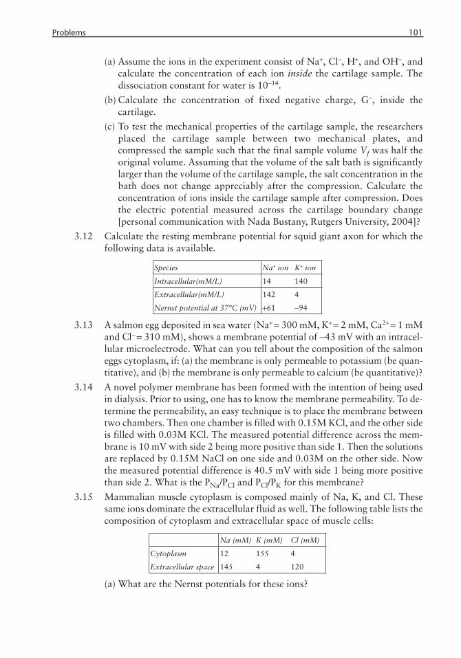
Problems 101
(a) Assume the ions in the experiment consist of Na+, Cl−, H+, and OH−, and calculate the concentration of each ion inside the cartilage sample. The dissociation constant for water is 1014.
(b) Calculate the concentration of fixed negative charge, G, inside the cartilage.
(c) To test the mechanical properties of the cartilage sample, the researchers placed the cartilage sample between two mechanical plates, and compressed the sample such that the final sample volume Vf was half the original volume. Assuming that the volume of the salt bath is significantly larger than the volume of the cartilage sample, the salt concentration in the bath does not change appreciably after the compression. Calculate the concentration of ions inside the cartilage sample after compression. Does the electric potential measured across the cartilage boundary change [personal communication with Nada Bustany, Rutgers University, 2004]?
3.12 Calculate the resting membrane potential for squid giant axon for which the following data is available.
Species Na+ ion K+ ion
Intracellular(mM/L) 14 140
Extracellular(mM/L) 142 4
Nernst potential at 37°C (mV) +61 −94
3.13 A salmon egg deposited in sea water (Na+ = 300 mM, K+ = 2 mM, Ca2+ = 1 mM and Cl− = 310 mM), shows a membrane potential of −43 mV with an intracel-lular microelectrode. What can you tell about the composition of the salmon eggs cytoplasm, if: (a) the membrane is only permeable to potassium (be quan-titative), and (b) the membrane is only permeable to calcium (be quantitative)?
3.14 A novel polymer membrane has been formed with the intention of being used in dialysis. Prior to using, one has to know the membrane permeability. To de-termine the permeability, an easy technique is to place the membrane between two chambers. Then one chamber is filled with 0.15M KCl, and the other side is filled with 0.03M KCl. The measured potential difference across the mem-brane is 10 mV with side 2 being more positive than side 1. Then the solutions are replaced by 0.15M NaCl on one side and 0.03M on the other side. Now the measured potential difference is 40.5 mV with side 1 being more positive than side 2. What is the PNa/PCl and PCl/PK for this membrane?
3.15 Mammalian muscle cytoplasm is composed mainly of Na, K, and Cl. These same ions dominate the extracellular fluid as well. The following table lists the composition of cytoplasm and extracellular space of muscle cells:
Na (mM) K (mM) Cl (mM)
Cytoplasm 12 155 4
Extracellular space 145 4 120
(a) What are the Nernst potentials for these ions?
Madihally_Book_2.indb Sec1:101Madihally_Book_2.indb Sec1:101 3/4/2010 5:23:52 PM3/4/2010 5:23:52 PM

102 Bioelectrical Phenomena
(b) The sum of the cation concentrations does not equal the chloride concen- tration on either side of the membrane. Why?
3.16 The potential difference across a cell membrane from outside to inside is ini-tially −90 mV (when in its resting phase). When a stimulus is applied, Na+ ions are allowed to move into the cell such that the potential on the inside changes to +20 mV for a short amount of time (depolarization time).
(a) If the membrane capacitance per unit area is 1 mF/cm2, how much charge moves through a membrane of area 0.05 cm2 during the depolarization time?
(b) The charge on a Na+ ion is positive. How many ions move through the membrane?
(c) How much energy is expended in moving these ions through the membrane to create this change in potential (called the action potential)?
3.17 If the time constant of a typical axon is 10 ms, what would be the resistance of one square centimeter of its membrane? The membrane capacitance of a typical axon is 1 mF/cm2.
3.18 Dr. Shingo Yashu is studying a neuromusclular interaction using voltage clamp measurements. He is interested in using tetraethylammonium (TEA) to block potassium conductance.
(a) To understand the output, he needs to derive a potassium conductance equation using the Hodgkin-Huxley model. Please help him.
(b) A part of a muscle cell membrane was studied with the voltage clamp measurements with a 30-mV positive voltage step input. He measured the membrane current as 0.5 mA/cm2 after 5 ms of step input. When the potassium current was blocked with TEA the current was 1 mA/cm2 after 5 ms of step input. Also, he observed that the flow of K+ ions could be stopped with a 100-mV increase in resting membrane potential. What is the potassium ion conductance gK?
3.19 The axons of the myelinated nerve fibers are completely encased in a my-elin sheath. Their neural conduction rates are faster than those of the un-myelinated nerve fibers. Myelinated nerve fibers are present in somatic and autonomic nerves. In a patient, one of the myelinated nerves was damaged in their right arm, which reduced the propagation speed to 65% of the original. Damaged and healthy nerves are stimulated with a similar stimulus current. If the smallest current adequate to initiate activation is considered to remain unchanged, how much longer is stimulus needed with the damaged nerve? The propagation speed is inversely proportional to the square root of the mem-brane capacitance
12( ( ) )mCα −Θ .
3.20 A membrane has 75 Na+ ion channels/mm2 with a conductance of 4 pS/chan-nel. The capacitance of the membrane is 0.01 pF/mm2. Calculate the flow and the time of sodium ions across the membrane of surface area of 1 mm2 with VM = −65 mV, VM
’ = 35 mV, and VNa = 62 mV.
3.21 A defibrillator detects ventricular fibrillation, and shocks the heart to restore the normal rhythm. Phillips is interested in manufacturing a new defibrillator
Madihally_Book_2.indb Sec1:102Madihally_Book_2.indb Sec1:102 3/4/2010 5:23:54 PM3/4/2010 5:23:54 PM

Problems 103
using a 40-mF capacitor charged with an adjustable power supply capable of generating a high voltage between 0 and 2,500V. The capacitor discharges through the patient, who is represented by the equivalent resistance R at the time of defibrillation.
(a) What is the value of the voltage for the energy accumulated in the capacitor to be equal to 100J?
(b) With the high voltage set to the value found in (a), how long will it take for the capacitor voltage to decrease to the value 10V? Assume that the resistance of the patient is 50W.
(c) If the cycle time between two shocks is set for 20 seconds, what is the residual voltage at the end of 20 seconds? Do you see accumulation of voltage for 10 shocks?
3.22 During defibrillation, Marcus measured the supplied current in a patient for the defibrillator voltage. The obtained profiles are shown in the figure. Based on the graphs
(a) Estimate the patient’s resistance. Do you think that the patient’s body has a constant resistance? Validate your answer.
(b) Derive the relation between voltage and time for the 0 to 1 ms interval, the 1 and 5 ms interval, and the 5 to 6 ms interval.
(c) Use the results in part (b) to derive the equations for the current in the three intervals.
(d) Draw the graph for the product IΔφ as a function of time t between 0 and 6 ms. (The product IΔφ is the power in watts delivered to the patient at any instant of time.) Estimate the area under the curve of IΔφ, which is equal to the total energy (in joules) delivered to the patient.
Madihally_Book_2.indb Sec1:103Madihally_Book_2.indb Sec1:103 3/4/2010 5:23:56 PM3/4/2010 5:23:56 PM

104 Bioelectrical Phenomena
3.23 The membrane potential can be written as ΔΦ = Q/C, where C is the mem-brane capacitance. For the value of C we found, C = 1.3 10−11 Farads, show that the charge Q needed to generate a −70 mV potential drop across the membrane is very small compared to the bulk concentrations of Na+ and K+. The bulk concentrations are Na+(out) = 145 mM, Na+(in) = 15 mM, K+(out) = 5 mM, and K+(in) = 145 mM. Hint: ρ = z.F.c [personal communication with Nada Bustany, Rutgers University, 2004].
3.24 In a spherical neuron soma, the values of the conductances to the three main ions were estimated to be: GNa = 40 pS, GK = 700 pS, GCl = 250 pS. What is the total membrane resistance?
3.25 A pacemaker (or “artificial pacemaker” not to be confused with the heart’s natural pacemaker), is a medical device designed to regulate the beating of the heart. It can be designed as a simple RC device that sends a pulse to a pa-tient’s heart every time the capacitor in the pacemaker is charged to a voltage of 0.23V. In a typical design, a pacemaker with a 110-μF capacitance and a battery voltage of 3.0V is used. If 60 pulses per minute are needed, what is the value of the resistance? What is the expected lifetime of such a battery if a typical current of 5 μA is produced and the battery supplies a charge of 0.4 ampere-hour?
3.26 Consider the RC circuit loop shown in the figure and a magnification of the capacitor in the circuit, showing an enclosed volume around one plate of the capacitor. At the capacitor, the principle of conservation of charge states that the rate of change of charge Q, dQ/dt, enclosed within the dotted volume is equal to Iin − Iout, where Iin is the current entering the enclosed volume and Iout is the current leaving the volume. Thus, dQ/dt = Iin − Iout.
(a) Using this conservation of charge principle, derive an expression for ic in the circuit as a function of the capacitance C, and ΔφC, the voltage drop across the capacitor. Note that Q = CΔφC for a capacitor.
(b) Using Ohm’s law across the resistor, and Kirchoff’s current and voltage laws, write a differential equation for ΔφC = Δφ1 − Δφ2= ΔφR.
(c) From (b), solve for ΔφC(t). Plot ΔφC as a function of time and as a function of Δφo = Δφ(t = 0) [personal communication with Nada Bustany, Rutgers University, 2004].
3.27 The circuit loop in Problem 3.26 is connected to a current source Is, which outputs a current I into the loop. The forcing current, I, is a step function and
Madihally_Book_2.indb Sec1:104Madihally_Book_2.indb Sec1:104 3/4/2010 5:23:58 PM3/4/2010 5:23:58 PM
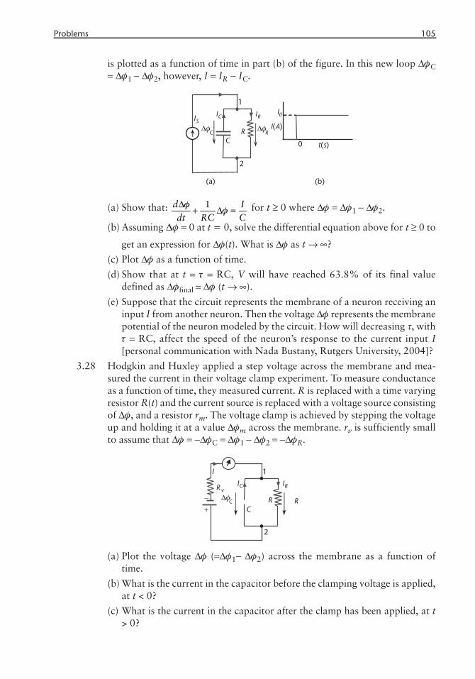
Problems 105
is plotted as a function of time in part (b) of the figure. In this new loop ΔφC = Δφ1 − Δφ2, however, I = IR − IC.
IC
1
CC
(a)
R
2
IR
R
t s( )
I0
0
ISI A( )Δφ Δφ
(b)
(a) Show that: 1d Idt RC C
φφ
Δ+ Δ = for t ≥ 0 where Δφ = Δφ1 − Δφ2.
(b) Assuming Δφ = 0 at t = 0, solve the differential equation above for t ≥ 0 to
get an expression for Δφ(t). What is Δφ as t → ∞?
(c) Plot Δφ as a function of time.
(d) Show that at t = τ = RC, V will have reached 63.8% of its final value defined as Δφfinal = Δφ (t → ∞).
(e) Suppose that the circuit represents the membrane of a neuron receiving an input I from another neuron. Then the voltage Δφ represents the membrane potential of the neuron modeled by the circuit. How will decreasing , with τ = RC, affect the speed of the neuron’s response to the current input I [personal communication with Nada Bustany, Rutgers University, 2004]?
3.28 Hodgkin and Huxley applied a step voltage across the membrane and mea-sured the current in their voltage clamp experiment. To measure conductance as a function of time, they measured current. R is replaced with a time varying resistor R(t) and the current source is replaced with a voltage source consisting of Δφ, and a resistor rm. The voltage clamp is achieved by stepping the voltage up and holding it at a value Δφm across the membrane. rv is sufficiently small to assume that Δφ = −ΔφC = Δφ1 − Δφ2 = −ΔφR.
(a) Plot the voltage Δφ (=Δφ1− Δφ2) across the membrane as a function of time.
(b) What is the current in the capacitor before the clamping voltage is applied, at t < 0?
(c) What is the current in the capacitor after the clamp has been applied, at t > 0?
Madihally_Book_2.indb Sec1:105Madihally_Book_2.indb Sec1:105 3/4/2010 5:24:00 PM3/4/2010 5:24:00 PM

106 Bioelectrical Phenomena
(d) What is the current in the resistor after the clamp has been applied, at t > 0?
(e) Assuming that R(t) represents the voltage gated sodium channels, how do you expect the current measured by the current meter to vary as a function of time if the cell generated an action potential?
(f) What should the clamp voltage, Vm, be to elicit an action potential [per- sonal communication with Nada Bustany, Rutgers University, 2004]?
3.29 With δ = 5 nm, εm ~ εo = 8.85 · 10−12 Farads/m, and the radius of the cell, R = 25 m, calculate the capacitance, C, of the cell in units of Farads. Assume that the cell is a sphere and that the surface area of the cell is equal to the surface of the capacitor plate.
3.30 An air-filled parallel plate capacitor has a capacitance of 5.0 pF. A potential of 100V is applied across the plates, which are 1.0 cm apart, using a storage battery. What is the energy stored in the capacitor? Suppose that the battery is disconnected and the plates are moved until they are 2.0 cm apart. What is the energy stored in the capacitor now? Suppose, instead, that the battery is left connected and the plates are again moved until they are 2.0 cm apart. What is the energy stored in the capacitor in this case?
3.31 Wie wants to modify a defibrillator by replacing the capacitor inside of it with another one. Assume the capacitor is a simple parallel-plate capacitor.
(a) If we wanted a “bigger” capacitor, one that could store more charge per volt of potential difference, would we want to increase or decrease the sur- face area of the capacitor’s plates?
(b) If we wanted a capacitor with double the capacitance of the original, 64- mF capacitor, by what factor would we want the area of the plates in- creased or decreased?
(c) What if a 32-mF capacitor with 5,000V is used?
(d) Suppose we successfully have replaced our original 64-mF capacitor with a 128-mF capacitor. How high would the voltage have to be to apply the same charge to the patient? How much energy would then be discharged through the patient?
3.32 Instead of changing the area (which would be difficult to do without more material), we could try to change the separation of the plates.
(a) In order to increase the capacitance, should we try to separate the plates more, or should we try to squeeze them closer together?
(b) Suppose we squeezed the original capacitor so that the distance between the plates became 1/4 of what it was originally. What would the new capacitance be?
Selected Bibliography
Aidley, D. J., The Physiology of Excitable Cells, 4th ed., New York: Cambridge University Press, 1998.
Madihally_Book_2.indb Sec1:106Madihally_Book_2.indb Sec1:106 3/4/2010 5:24:02 PM3/4/2010 5:24:02 PM

Problems 107
Bronzino, J. D., (ed.), The Biomedical Engineering Handbook, 2nd ed., Boca Raton, FL: CRC Press, 1999.Gillis, K. D., “Techniques for Membrane Capacitance Measurements,” in Sakmann, B., and E. Neher, (eds.), Single-Channel Recording, 2nd ed., New York: Plenum Press, 1995, pp. 155–198.Gulrajani, R. M., Bioelectricity and Biomagnetism, New York: John Wiley & Sons, 1998.Hille, B., Ionic Channels of Excitable Membranes, 3rd ed., Sunderland, MA: Sinauer Associates, 2001.Hodgkin, A. L., and A. F. Huxley, “A Quantitative Description of Membrane Current and Its Application to Conduction and Excitation in Nerve,” Journal of Physiology, Vol. 117, 1952, pp. 500–544.Koch, C., Biophysics of Computation: Information Processing in Single Neurons, New York: Oxford University Press, 2004.Malmivuo, J., and R. Plonsey, Bioelectromagnetism, New York: Oxford University Press, 1995.Fall, C. P., et al., Computational Cell Biology, New York: Springer, 2005. Plonsey, R., and R. C. Barr, Bioelectricity, New York: Plenum Press, 1988.Webster, J. G., Medical Instrumentation: Application and Design, New York: John Wiley & Sons, 2000.
Madihally_Book_2.indb Sec1:107Madihally_Book_2.indb Sec1:107 3/4/2010 5:24:04 PM3/4/2010 5:24:04 PM

Madihally_Book_2.indb Sec1:108Madihally_Book_2.indb Sec1:108 3/4/2010 5:24:06 PM3/4/2010 5:24:06 PM


![Cooperative elastic switching vs laser heating in [Fe(phen ... · The thermal phase transition of [Fe(Phen) 2 (NCS) 2] crystals was intensively investigated by different spectroscopic](https://static.fdocuments.us/doc/165x107/60a67fd7816aa0047a1ed84a/cooperative-elastic-switching-vs-laser-heating-in-fephen-the-thermal-phase.jpg)


