BIODIVERSITY AND BIOLOGY OF MARINE ORNAMENTAL REEF FISHES...

ASSESSMENT AND CONSERVATION OF BIODIVERSITY USING REMOTE SENSING AND GEOGRAPHIC INFORMATION SYSTEM (GIS)

M.C. Gupta Remote Sensing Application Centre

Madhya Pradesh Council of Science and Technology Bhopal - 462 003

ABSTRACT

During, late 20th Century, the humans are coming to realize that the biological resources in landscapes have limits of exploitation and that we are exceeding these limits thereby depleting the biological resources and their diversity at a level which is irreversible. This is, therefore, a time of change not only in the attitude of the present society but also in the relationship between people and the natural resources upon which their welfare depends. Species are becoming extinct at the fastest rate known in geological history and climate appears to be changing more rapidly than ever before. The sustainable management of biodiversity has become a key issue for survival of man on the planet Earth. In this effort conservation of landscape biodiversity has been put to the highest priority.

India is one among the top twelve mega-diversity countries in the world in terms of biodiversity. There is direct relationship between biodiversity and bioproductivity. The North Eastern region of India occupies nearly 7.7% of the geographical area of the country comprising most diverse flora and fauna. The human interventions in the North Eastern region through developmental activities and shifting cultivation have resulted in deforestation. The age-old practice of shifting cultivation and lumbering was a major

Biodiversity : Life to our mother earth

2

cause of extensive changes in biodiversity in Papumpare District of Arunachal Pradesh in North Eastern region. Reduction in jhum cycle to 3–5 years as compared to 20–30 years earlier due to increase in human population has accelerated the process of landscape biodiversity changes leading to degradation and fragmentation with poorer species composition with the passage of time.

INTRODUCTION

Landscape biodiversity are important yet they are very poorly understood. Awareness on importance of spatial heterogeneity of a landscape biodiversity and interactions among various landscape elements is the first step in developing our understanding of landscape. Landscape commonly refers to the landforms of a region in the aggregate or to the land surface and its associated habitats at scales of hectares to many square kilometers. Geomorphic processes, colonization by the organisms and disturbances mould the structure of the landscapes. The landscape biodiversity, therefore, focuses on the structure and spatial patterns of landscape elements, the function, that is, flow of energy and material among landscape elements and the change in structure and function in space and time. Landscapes show a common fundamental structure of patches, corridors and matrices. They also involve a whole lot of biological diversity species, nutrients and materials all of which contribute to the landscape biodiversity dynamism.

Remote Sensing and GIS have proved to be very effective tools to analyse biodiversity at various levels i.e., macro level, meso level and micro level. Different types of land covers make patches or elements of the landscape.


3

Various parameters of patch characteristics like fragmentation, porosity, patchiness and interspersion are directly influenced by parent material like rock, soil, climate and human activities. Thus, remote sensing is an important observation and measurement tool for analysis of landscape biodiversity. It offers the capability to collect data on landscape biodiversity characteristics. The multispectral, multitemporal and multiscaled attributes of the remotely sensed landscape can provide a look of biophysical and land cover components that previously was unachievable.

The identification and measurement of landscape variables from remotely sensed data include a range of interpretation techniques of satellite data to advanced image processing algorithms. One of the greatest benefits of applying remote sensing to landscape biodiversity, however, is the ability to measure the state and dynamics of ecological variables and the processes that derive these variables. Within a GIS framework, the extrapolation of remotely sensed information from point sources to spatially large scales will enhance the capabilities for modeling landscape biodiversity properties.

STUDY AREA

Present study area, the Papumpare District of Arunachal Pradesh, lies between North latitudes 26o56’36”

and 27o38’22” and East longitudes 93o12’ and 94o12’. The height of the elevation of study area lies between 200 meters and 3,600 meters at mean sea level. The Papumpare dist., is bounded by Lower Subansiri District in the North, Assam State in the South and South East and by the East Kameng District in the West. The Papumpare District is in many ways, a land of extremes. There lies the Apatani Valley presenting a rich biodiversity.


4

The Papumpare District is divided into two sub divisions viz; Itanagar and Sagalee. Itanagar sub division is comprised of Doimukh – Kimin Block consisting of five circles, namely; Kimin, Doimukh, Balijan, Naharlagun and Itanagar. Sagalee sub division is comprised of Sagalee Block consisting of Sagalee and Mengio Circles. The total area of the district is 2,875 Km. inhabited by 252 villages having population of 72,811 (population density 25/Km).

Papumpare District falls in Western forest circle consisting of one territorial division, six functional division and 19 ranges. The District consists of 810.50 Km, of reserved forest, 140.30 Km, wildlife sanctuary, 315.69 Km, under proposed reserved forest, thus, total forest area is 1266.49 Km.

NATURAL RESOURCES SETTING

Geology

High-grade metamorphic rocks like biotic, garnet, silimanite and graphite schists, migmatites and intrusions of pegmatite, tourmaline granite are seen. These rocks appear to be folded into synform and antiform.

Soil

The nature and type of soil vary with topography and climate of the District. Generally the soil is loose, sandy loam mixed with pebbles. In the region extending from the foothills up to approximately an altitude of 762 meters the soil varies from sandy to loamy. In the upper region beyond the altitude of 762 meters the soil varies from loamy to clayey with a thick layer of humus at the top. Thick humus is


5

found in areas, which are covered with evergreen forests, whereas the areas with scanty vegetation are having only a few centimeters of topsoil over rocks. The base of the valley consists of gnesis and schist overlaid on a wide area with almost horizontally disposed older alluvial deposits comprising partially consolidated bed gravels, interbedded sand, girt, loam clay and peat. On the hills, the soils have developed mostly on shales, sandstone, quartzite and phyllile. Very thick deposits of medium and fine sand with round and semi round rock fragments and boulders below the soil depth were found.

River System

Dikrang, Panyor and Ranga are the main rivers and Panchin, Senkhi, Shupabung, Par, Rachipabung, Niyarpungpabung, Pering, Payan, Kund are the tributaries nala of the study area.

Fauna

Small animals include flat worms, round worms, earth worms, leeches, millipedes, centipedes, crabs, prawns, spiders, scorpions, various kinds of insects, shells, slugs, snakes, lizards and bats. Big animals like tigers, elephants, deer, primates, insectivores, rodents and birds were found.

DATA AND MATERIAL

Primary Data

Indian Remote Sensing Satellite (IRS – IC LISS III), standard false colour composite (FCC 4,2,3 band) on


6

1:250,000 scale (Path 111, Row 52, Path 112, Row 52) hard copy.

Secondary Data

Survey of India (SOI) toposheet number 83 E, F and I. Census Maps (circle boundary) to draw the District Map and Circle Map of Papumpare District. Census Data for population, climatic data for ombrothermic diagram. The present study was done on INTERGRAPH GIS software.

METHODOLOGY

Preparation of Base Map

Base Map of Papumpare District was prepared on 1:250,000 scale using Survey of India degree sheets (83 A, E, F and I). Roads, major rivers, major settlements and other permanent features were transferred from degree sheet to base map. The study area boundary (Papumpare) was prepared by mosaicing of circle boundary maps obtained from census department. Scale was adjusted using Pantagraph.

Preparation of Contour and Drainage Map

Using the above mentioned degree sheets, the contours on 200 m, interval were drawn. These contours were used to generate Digital Elevation Model (DEM). The drainage was also prepared using degree sheets. Maps were scanned on scanner and were on screen digitised using GEOVEC Software in INTREGRAPH.

Pre field visual interpretation of Satellite Imagery


7

The pre field visual interpretation was done with existing imageries. Using various elements of image interpretation viz., tone, texture, size, shape, location, pattern, association etc. Different landcovers and cultural features were demarcated as polygons. The doubtful areas for specific locations were marked for field checks.

Reconnaissance Survey

Reconnaissance Survey of the area was done for getting patterns of vegetation and other land features in the area. Major vegetation types and other landcover characteristics were covered and identified on both toposheets and imagery. Observations were made for the variation of tonal pattern and textural patterns of FCCs. Traverses were made along the roads, major drainages, hilltops, and valley, and inside forested area for collecting ground truth. Existing literature study and interaction with forest department and local research institutes were also done for information on scientific line.

Preparation of Interpretation Key

Based on reconnaissance survey of the ground details and imageries signatures, interpretation key was developed to extract information from the image.

Ground Truth

Ground truth verification was done with the help of toposheets on 1:50,000. For ground truthing of doubtful areas, care was taken to cover all types of features identified on image. As much as possible, traverses were made to


8

include all gradients of latitudinal and altitudinal variables. For inaccessible areas, discussions were made with the forest department and forest research institute and accordingly maps were finalised.

Phytosociological and biodiversity Study Sampling

Stratified random sampling was done for analysis of vegetation composition of all types. Species area curve was the basis for determining the size of the quadrat in each forest type where the number of species becomes constant for atleast 3 consecutive stages. By experimentation it was found that 20m x 20m quadrats were the appropriate size for the Phytosociological and biodiversity sampling for the present study.

For each life form number of individuals were recorded. For each vegetation type the field data was analyzed for computation of importance value index (IVI), which is the sum of Relative density, Relative frequency and Relative dominance.

Total Number of quadrats in which species occur Frequency= x 100 Total number of quadrats studied

Total Number of individuals of the species occuring Density = x 100 (per quadrat) Total number of quadrats studied

Total Number of individuals of species occuring Abundance = x 100 Total number of quadrats in which species occur

Frequency of a species Relative Frequency = x 100


9

Sum of frequency of all the species

Density of a species Relative Density = x 100 Sum of density of all the species

Total stand basal cover of the species

Relative domiance = x 100 Total stand basal cover of all the species

Basal cover = (cbh)²/4π Sum of basal cover of individual plants of a species will yield total stand basal cover of that species.

Mean basal cover = Stand basal cover/density

Importance Value Index (IVI) =

Relative Frequency + Relative Density +Relative Dominance

Species Richness (Diversity) Species Diversity – Shannon – Wiener Index (H) H = -Σ [(ni/N) log 2 (ni/N] (where log implies to log base 10)

Where H is the index value and ‘ni’ importance value or number of species and ‘N’ is total IVI or total number of species in that habitat type. It is also called Information Index and was used to describe the landscape biodiversity.

The larger the value, higher the H’ and more diverse the landscape.

Digital Elevation Model


10

Digital Elevation Model was generated using the contour map and forest/vegetation map was draped on Digital Elevation Model to feel the real virtuality about landscape biodiversity.


11

Road Buffer Map

The Road Buffer Map was generated at 500 meters interval using Transport network and settlement map to establish the disturbance gradient upto 1.5 kilometers.

RESULT

Forest/Vegetation Mapping In order to carry out the landscape biodiversity

analysis of the District, vegetation/forest type map was prepared by visual interpretation of IRS 1C L ISS III hard copy paper print satellite data. Apart from type mapping, density level classification was also done. Forest type has been classified as dense forest (crown cover > 40%) and open forest (crown cover < 40%). The vegetation has an altitudinal distribution and may be broadly classified into four main types : (I) Tropical Semi Evergreen Forests, (II) Sub Tropical Evergreen Forests, (III) Derived Grassland (Shifting Cultivation) and (IV) Temperate Forests.

(I) Tropical Semi Evergreen Forests (Upto 900 m)

These forests extend upto a height of 900 m. The top storey is formed by tall trees, such as Dipterocarpus macrocarpus (‘Hollong’). Artocarpus chaplasha, Tetrameles nudiflora, Altingia excelsa, Terminalia chebula, Bombax ceiba, Chukrasia tabularis, C. velutina. Lagerstroemia speciosa, Bischofia javanica, Dysoxylum procerum, Castanopsis indica, Solanea assamica, Amoora wallichii, Callicarpa arborea, Cinnamomum cecicodaphne, Dillenia indica, Duabanga sonneratioides, Mangolia campbellii,


12

Pterospermum acerifolium, Quercus glauca and Shorea assamica. The next storey is represented by small trees, namely, Mesua ferrea, Phoebe goalparensis, Duabanga grandiflora, Eugenia formosa, Goniothalamus simonsii, Talauma hodsonii, Dillenia indica, Illicium griffithi, Michelia dolltsopa, Bauhinia purpurea, Ficus hispida and Syzygium pseudoformosum. The canes, mostly Calamus leptospadix and C. erectus occurring in swamps and forming impenetrable thickets, are met within these forests. Tree ferns Cyathea spp. and large fern Angiopteris erecta are found associated with Pondanus furcatus. The wild banana Musa balbisiana is a conspicuous feature of these forests.

The common shrubs met within these forests are Abroma augusta, Ardisia humilis, A. undulata, Capparis acutiflia, Sabiafolia spp., Micromelum roxburghii, Solanum torvum, Cerodendrum glandulosum, C. serratum, C. villosum and Boecia fulva. The ground flora is represented by Achyranthes bidentata, Alternanthera sessilis, Commelina paludosa, Murdania nudiflora, Polygonum barbatum, P. serrulatum, Oxalis corniculata and many species of ferns and fern allies like Asplenium, Equisetum and Selaginella. The epiphytes include ferns, fern allies, orchids and members of families Gesneriaceae and Zingiberaceae. Balanophora dioica, a fleshy root parasite on the roots of trees, is occasionally seen in shady, moist and humus covered areas of the forest.

(II) Subtropical Evergreen Forests (900–1,800 m)

These forests are dominated by Schima wallichii, Callicarpa arborea, Actinodaphne obovata, Alnus nepalensis, Castanopsis indica, Bauhinia variegata, Eurya


13

acuminata, Byttneria aspera, Evodia fraxinifolia, Ficus gasparriniana, Kvdia calycina, Magnolia pterocapra, Prunus nepalensis and Saurauia punduang. Among smaller trees Photinia notoniana and Alphania rubra are common. The common shrubs and under shrubs in these forests are Berberis wallichiana, Mahonia nepalensis, Agapetes auriculata, A. buxifolia, Vernonia saligna, Tephrosia candidida and Viburan foetidum. The climbing shrubs are represented by Clematis acuminata, Holboellia latiflia and Tinospora malabarica. The herbaceous flora includes Anaphalis odorata, Anemone vitifolia, Plantago erosa and Viola serpens.

(III) Shifting Cultivation/Grasslands (Upto 1,000 – 1,500 m)

These make their appearance where both the Subtropical forests and the grasslands are found to co-exist. The grasslands owe their origin to the practice of jhuming (shifting cultivation). As the name suggests, there are number of grasses such as Arundinella bengalensis, Saccharum arundinaceum, S. spontaneum, Setaria palmifolia, Neryaundia reynaudiana and Thysanolaena maxima. Several species of bamboos are found in this region, such as Cephalostachyum latifolium, Chimnobambusa callosa and Phyllostachys bambusoides. Some scattered trees, namely, Bombax ceiba, Syzygium cumini and Sterculia villesa were also found.

(IV) Temperate Evergreen Forests (1,800 – 3,500 m)

The dominant families represented here are Coniferae, Cupuliferae, Ericaceae and Magnoliaceae. Oaks


14

show fairly distinct altitudinal zonation. The chief trees are species of Quercus, Castanopsis, Acere, Magnolia, Michelia, Pyrus and Prunus. In many parts Quercus and in some places bamboos like Cephalostachyum form pure stands. From the height of 2,600 m and above, Taxus baccata was found among common species on the north and eastern slopes. Abies spectabilis, Cupressus torulosa and Tsuga dumosa may also be mentioned. A few common herbs in the temperate region are Gerbera rilloselloides, Polygonum molle, Urtica parviflora and Viola patrinli.

Agriculture

The methods of agriculture practiced by the people, depending on ecological conditions are of three types, namely, shifting cultivation or jhum, permanent or sedentary agriculture and partly shifting cultivation and partly sedentary. Maize, rice, finger millet are major crops grown in the district. Other crops are wheat, potato, mustard, pulses, vegetables, etc.

Settlement

Bigger settlements like Itanagar, Doimukh and Kimin are identified on the image.

Drainage Map

The drainage is subdendritic to parallel in nature. The drainage density is moderately high-to-high in valley portion. Drainage of first to third order with annual to perennial in nature are seen in the district.


15

Area Statistics of Forest Vegetation Map

The total geographical area of the District is 3,437 Km2. Tropical evergreen closed forest is represented by 599 Km2, which is 17.5% of the total geographical area. However, tropical semievergreen open forest is represented by 143.5 Km2, which was 4.17% of the total geographical area. The Subtropical evergreen closed and open forest was occupied by 10,641 Km2 and 420 Km2 respectively, which was 31% and 12.2% of the total geographical area. Temperate evergreen closed and open mixed forest was occurring in 1021.5 Km2 and 45.5 Km2 respectively, which was 29.7% and 1.3% respectively of total geographical area. The grasslands, which have originated from shifting cultivation was represented by 18.24 Km2, which was 0.53% of total geographical area. Agriculture land occurring mainly on the valley portion of the river coarse is 101.3 Km2, which is 2.96% of the total geographical area. The settlement was represented by 19.2 Km2, which is 0.56% of the total geographical area. The plantations occur in 2.01 Km2 area which is 0.06% of total geographical area (Table 1).

Table 1: Forest/Vegetation Area Statistics

Category Area in Sq.Km.

Geographical Area (%)

Tropical semi evergreen closed mixed forest

599.80 17.45

Tropical semi evergreen open mixed forest

143.52 4.17

Sub tropical evergreen 1064.96 30.98


16

Category Area in Sq.Km.

Geographical Area (%)

closed mixed forest

Sub tropical evergreen open mixed forest

420.35 12.23

Temperate evergreen closed mixed forest

1021.41 29.71

Temperate evergreen open mixed forest

45.41 1.32

Shifting cultivation 18.22 0.53

Agriculture 101.27 2.96

Plantation 2.01 0.058

Settlement 19.17 0.56

Fog 0.89 0.03

PHYTOSOCIOLOGICAL ANALYSIS AND BIODIVERSITY

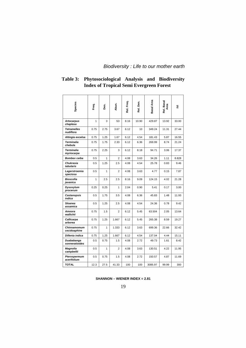
The Phytosociological Analysis of forest vegetation for frequency, density, dominance, basal area, relative frequency, relative basal area, relative dominance and importance value index (IVI) and Shannon – Wiener Index is given in Tables 2 and 3.


17

The Shannon – Wiener Index for tropical semi evergreen forests was 2.81, for sub tropical evergreen was 2.34 and for the temperate evergreen forest was 2.2. Shannon - Wiener Index follows the following decreasing trend: Tropical semi evergreen forest > sub tropical evergreen > temperate evergreen forest.


18

Table 2: Phytosociological Analysis And Biodiversity Index of Subtropical Evergreen Forest

Spec

ies

Freq

.

Den

.

Abu

n.

Rel

. Fre

q.

Rel

. Den

.

Bas

al A

rea

Rel

. Bas

al

Are

a

IVI

Schima wallichii

1 19.25 5 8.69 12.73 471.78 18.67 40.11

Actinodaphne obovata

1 19.31 3.25 8.69 12.77 474.85 18.8 40.27

Alnus nepalensis

1 14.75 5 8.69 9.76 276.99 10.96 29.42

Bauhinia variegata

1 13.88 4.75 8.69 9.18 245.10 9.70 27.58

Euryya acuminata

0.75 9.5 3.66 6.52 6.28 114.90 4.54 17.35

Bytneria aspera

0.75 7.75 3 6.52 5.12 76.46 3.02 14.67

Evodia fraxinifolia

1 13.25 2.75 8.69 8.76 223.51 8.84 26.31

Ficus gasparriniana

0.75 12.19 2.66 6.52 8.06 189.10 7.48 22.07

Kvdia calycina.

0.75 7.06 2 6.52 5.67 63.50 2.51 13.70

Magnolia pterocarpa

1 11.63 3 8.69 7.69 172.05 6.81 23.19

Saurauia punduang

1 8.37 1 8.69 5.54 89.30 3.53 17.77

Photinia notoniana

0.75 6.93 2.66 6.52 4.59 61.27 2.42 13.53

Alphanai rubra

0.75 7.25 1.33 6.52 4.79 66.92 2.64 13.96

TOTAL 11.5 151.1 40.08 100 100 2525.79 100 299.99

SHANNON – WIENER INDEX (H) = 2.34


19

Table 3: Phytosociological Analysis and Biodiversity Index of Tropical Semi Evergreen Forest

Spec

ies

Freq

.

Den

.

Abu

n.

Rel

. Fre

q.

Rel

. Den

.

Bas

al A

rea

Rel

. Bas

al

Are

a

IVI

Artocarpus chaplasa

1 3 S3 8.16 10.90 429.87 13.92 33.00

Tetramelles nudiflora

0.75 2.75 3.67 6.12 10 349.24 11.31 27.44

Altingia excelsa 0.75 1.25 1.67 6.12 4.54 181.43 5.87 16.55

Terminalia chebula

0.75 1.75 2.33 6.12 6.36 269.99 8.74 21.24

Terminalia myriocarpa

0.75 2.25 3 6.12 8.18 94.71 3.06 17.37

Bombex ceiba 0.5 1 2 4.08 3.63 34.26 1.11 8.828

Chukrasia tabularis

0.5 1.25 2.5 4.08 4.54 25.78 0.83 9.46

Lagerstroemia speciosa

0.5 1 2 4.08 3.63 4.77 0.15 7.87

Bioscofia javanica

1 2.5 2.5 8.16 9.09 124.15 4.02 21.28

Dysoxylum procerum

0.25 0.25 1 2.04 0.90 5.41 0.17 3.00

Castanopsis indica

0.5 1.75 3.5 4.08 6.36 45.83 1.48 11.93

Sloanea assamica

0.5 1.25 2.5 4.08 4.54 24.36 0.78 9.42

Amoora wallichii

0.75 1.5 2 6.12 5.45 63.504 2.05 13.64

Callicarpa arborea

0.75 1.25 1.667 6.12 5.45 265.38 8.59 19.27

Chinnamomum cecidoaphine

0.75 1 1.333 6.12 3.63 699.36 22.66 32.42

Dillenia indica 0.75 1.25 1.667 6.12 4.54 137.04 4.44 15.11

Duababanga sonneratioides

0.5 0.75 1.5 4.08 2.72 49.73 1.61 8.42

Magnolia campbellii

0.5 1 2 4.08 3.63 130.51 4.22 11.95

Pterospermum acerifolium

0.5 0.75 1.5 4.08 2.72 150.57 4.87 11.69

TOTAL 12.3 27.5 41.33 100 100 3085.97 99.99 300

SHANNON – WIENER INDEX = 2.81


20

LANDSCALE CHARACTERISATION

Fragmentation (Patchines) The Papumpare District due to relatively low population pressure and poor road network is still maintaining the original virgin forests, which are least disturbed. Following four fragmentation classes has been identified (I) Non Fragmented (96.6%), Highly Fragmented (1.66%), Medium Fragmented (1.91%) and Low Fragmented Area (0.04%).

Porosity

The porosity for evergreen and semi evergreen forest is estimated separately. Porosity classes of evergreen forests are: Non Porous (69.85%), Low Porosity (5.57%), Medium Porosity (1.71%), High Porosity (0.05%). The porosity of semi evergreen forests are: Non Porous (19.06%), Low Porosity (1.69%), Medium Porosity (2.52%) and High Porosity (0.2%).

Interspersion

Six interspersion classes viz., intact zone (96.83%), high interspection (0.03%), moderate (0.5%), medium (0.56%), low (0.89%) and lowest (1.19%) were identified.

DISCUSSION

Deforestation in Papumpare District has led to a landscape of isolated forest patches; the impact varies from species to species. The ongoing changes in landscape biodiversity patterns are mainly due to shifting cultivation (cutting forest and burning them during dry period for agriculture) alter the isolation of species differentially.


21

Change is characteristic of virtually all landscapes, but it is episodic and driven by social, economical and political factors. Predicting landscape biodiversity change is an ongoing challenge in many disciplines. In biodiversity, the challenge is to combine stand dynamics models with landuse dynamics models to project timber supplies. Reciprocally, agricultural economists are attempting to model how complex social, economic and political forces affect trends in agricultural acreage and their allocation to crops, pasture, natural vegetation (forest) and land uses. Other investigators are assessing the dynamics of landuse change at the urban interface.

Given the ongoing nature of landscape biodiversity change, we believe that the focus of the research in landscape ecology needs to be on how landscape dynamics interact with species tolerances in time and space. The effects of disturbances frequently vary spatially across a landscape, creating a heterogeneous mosaic. Some disturbances propagate spatially and may be enhanced or retarded by the pattern of the landscape. Forest fragments are samples of longer area of forest and may exclude partially distributed species that were present in the original area. The extent to which the forest fragments represent the original forest depends on the proportion of the landscape converted into non forest, the spatial arrangement of remaining fragments and the size of forest species. Deforestation will affect the representatives of forest fragments. In the present study, for example, low land forests in flatter areas are generally cleared before forest on step slopes. As a result, groups of species or complete communities may be eliminated. The reduction in forest area due to fragmentation will result in a decrease in population sizes of forest species. For species


22

with patchy distribution, the abundance in fragments will depend on the location and size of the fragments for species that naturally occur at high densities, population size may not be reduced to critically low numbers in forest fragments of reasonable size. Species occurring at low densities will suffer from considerable reduction in population size and may become sensitive to local extinction as a result of stochastic events or reduced genetic fitness.

Reduced forest sizes will also make fragments more assessable for logging, hunting and gathering which can also contribute to species loss (Turner 1987). Transformation of a large forest area into several fragments results in population sub division. Clearly, the effect of fragment isolation differs among species, depending upon their mobility and dispersal mechanism or pollination agent.

The susceptibility of species in isolated protected areas to random demographic factors and environmental functions may prove ultimately to be the most important factor in determining extinction risk. Anthropogenic influences are much greater in fragments and in porous area. However, to some extent this may be a function of the fact that smaller fragments are not perceived to be important for conservation. Pragmatic decisions will have then to be taken as to when the theoretical, very long term risks to biodiversity due to forest fragmentation, porosity and interspersion are outweighed by the financial, social and logistic advantages of smaller, more manageable reserves.

The present study of landscape analysis indicates that more research is needed to elucidate the relationship between landscape biodiversity heterogeneity and disturbance.


23


24

FUTURE RESEARCH

The diversity of species, the variety of their responses to changes in resources and the complex mechanisms needed to explain these interactions demonstrated that all landscape studies must limit the scope and scale of their measurements. But how can this be accomplished without sacrificing our ability to make reliable and interesting prediction? New techniques, similar to sensitivity and uncertainty analysis that allow the importance of different variable and mechanism taken would be evaluated before additional measurements are taken would be extremely useful for establishing realistic limits for landscape studies. Although sensitivity methods have been successfully applied in a variety of ecological studies (Gardner et al., 1990) these methods have yet to be generally and rigorously applied to spatial systems. Hierarchy Theory (Aller and Starr. 1982; O’Neill et al., 1986) predicts that complex systems including landscapes (Urban et al., 1987) should develop structures that are hierarchically organised, that is, patterns that show significant shifts with changes in scale. Although this effect has been observed in several empirical studies, including present landscape biodiversity characterization (Anderson 1971); Krummel et al., (1987), it remains a challenge to establish temporal and spatial scale at which specific mechanisms eg., variability in soil, topography, climate, economics, species life history attributes, etc., will have the most influences on our ability to measure and predict. If the power of the GIS is used to develop a best-fit between data and predictions, then the spatial display of prediction errors will not be useful. However, if data are divided into separate sets of models development, calibration and testing, then the


25

spatial attributes of models error will be extremely interesting.

The general relationships between biodiversity indices, ecological processes and scale needs more case studies to provide understanding of both the factors that create pattern and ecological effects of changing patterns of processes. These applications are of particular importance because changes in landscape patterns are now monitored through remote sensing technology and an understanding of the pattern process relationship will allow functional changes to be inferred.

Acknowledgement

The author acknowledges Shri Girja Prasad for the fieldwork and lab work.

REFERENCES

Aller, T.F.H. and Star,T.B.1982. Hierachy. University of Chicago press. Chicago.

Anderson, D.J. 1971. Spatial pattern in some Australian dryland plant communities. In G.P. Patil and W.E. Water. Eds. Statistical Ecology Vol. 1. PA. Pennsylvania State University Press, University Park, pp. 271-286.

Garner, R.H., Dale V.H. and O Neil, R.V. 1990. Error propagation and uncertainty in process modeling. In: Process modeling of forest growth responses to environmental stress Eds: R.K.Dixon, Meldahl, R.H.,


26

Rurak, G.A. and Warren, G.A.Portland, Oregon: Timber Press.

Krummel, J.R., Gardner, R.H., Sugihara, G., ONeil, R.V. and Coleman, P.R. 1987. Landscape patterns in distributed environment. Oikos. 48 : 321-324.

ONeil, R.V., DeAngelis, D.L., Waide, J.B. and Allen, T.F.H. 1986. A hierarchical concept of ecosystem. Princeton, N.J., Princeton University Press.

Turner, M.G. 1987. Landscape heterogeneity and disturbance. Springer Verlag, New York.

Urban, D.L., O Neil R.V. and Shugart, H.H. 1987.Landscape Ecology, Bioscience. 37 : 119-127.

White, P.S.and MacKenzie, M.D. 1986. Remote Sensing and Landscape pattern in Great Somy mountain National Park biosphere Reserve, North Carolina and Tennesee In: Coupling of ecological studies with Remote Sensing : Potentials at four Biosphere Reserves in United State. Eds. Dyer, M.I. and Crossely Jr. U.S. Dept. of State Pub.

BIODIVERSITY AND BIOLOGY OF MARINE ORNAMENTAL REEF FISHES...

Documents

Transcript of BIODIVERSITY AND BIOLOGY OF MARINE ORNAMENTAL REEF FISHES...