Biochemical Engineering

James M. Lee

eBook Version 2.32

Use Bookmarks to go to the specific section of the ebook You can turn on the navigation panel by clicking Bookmark icon on the left panel.

Official web site of this ebook: http://jmlee.net Printing Guide (Printable Version Only)

x This file is only for your own use. You are not allowed to give this file to others by any means without permission in writing from the author. You are authorized to print one copy (or its replacement) for your own use.

x If an instructor (or student book store) is printing multiple copies to sell to students with the permission from the author, the royalty ($10 per copy) has to be paid to the author. It is the instructor's responsibility to ensure that his/her book store pay the royalty to the author by sending the check or paying through the purchase site (http://jmlee.net).

x If your printer allows you to scale your output, you may use 90-94% scaling for the best result. You can set it by changing the advanced option of your laser printer.

x It will be best if you print both side of paper, which can be done by printing even side first (by selecting the option in Adobe Reader Printing Option). When you print odd side, be sure to put papers into your printer in a right orientation. Test it by printing first 4 pages (page 2 to 6).

x You can also print a specific chapter by specifying the page range. Note the page range at the bottom of the Adobe Reader frame.

http://jmlee.org

Biochemical Engineering

James M. Lee

Washington State University

eBook Version 2.32

ii

© 2009 by James M. Lee, Department of Chemical Engineering, Washington State University, Pullman, WA 99164-2710. This book was originally published by Prentice-Hall Inc. in 1992.

All rights reserved. No part of this book may be reproduced, in any form or by any means, without permission in writing from the author.

iii

Contents Preface Chapter 1 Introduction

Importance of bioprocessing and scale-up in new biotechnology. Chapter 2 Enzyme Kinetics

Simple enzyme kinetics, enzyme reactor, inhibition, other influences, and experiments

Chapter 3 Immobilized Enzyme Immobilization techniques and effect of mass transfer resistance

Chapter 4 Industrial Applications of Enzymes Carbohydrates, starch conversion, cellulose conversion, and experiments

Chapter 5 Cell Cultivations Microbial, animal, and plant cell cultivations, cell growth measurement, cell immobilization, and experiments

Chapter 6 Cell Kinetics and Fermenter Design Growth cycle, cell kinetics, batch or plug-flow stirred-tank fermenter, continuous stirred-tank fermenter (CSTF), multiple fermenters in series, CSTF with cell recycling, alternative fermenters, and structured kinetic models

Chapter 7 Genetic Engineering DNA and RNA, cloning of genes, stability of recombinant cells, and genetic engineering of plant cells

Chapter 8 Sterilization Sterilization methods, thermal death kinetics, design criterion, batch and continuous sterilization, and air sterilization

Chapter 9 Agitation and Aeration Basic mass-transfer concepts, correlations form mass-transfer coefficient, measurement of interfacial area, correlations for interfacial area, gas hold-up, power consumption, oxygen absorption rate, scale-up, and shear sensitive mixing

Chapter 10 Downstream Processing Solid-liquid separation, cell rupture, recovery, and purification

iv

Preface to the eBook Edition While I was revising the book for the second edition, I decided to test this concept of college textbook as ebook. If it works out, more professors will be encouraged to try this concept and people will be benefited with variety of textbooks available as ebook inexpensively compared to the published books.

There are many other advantages for publishing textbooks as ebook including easy revisions and corrections, wide exposure of the text as a reference to general public, etc.

James M. Lee

v

Preface to the First Edition This book is written for an introductory course in biochemical engineering normally taught as a senior or graduate-level elective in chemical engineering. It is also intended to be used as a self-study book for practicing chemical engineers or for biological scientists who have a limited background in the bioprocessing aspects of new biotechnology.

Several characteristics lacking in currently available books in the area, therefore, which I have intended to improve in this textbook are: (1) solved example problems, (2) use of the traditional chemical engineering approaches in nomenclature and mathematical analysis so that students who are taking other chemical engineering courses concurrently with this course will not be confused, (3) brief descriptions of the basics of microbiology and biochemistry as an introduction to the chapter where they are needed, and (4) inclusion of laboratory experiments to help engineers with basic microbiology or biochemistry experiments.

Following a brief introduction of biochemical engineering in general, the book is divided into three main sections. The first is enzyme-mediated bioprocessing, which is covered in three chapters. Enzyme kinetics is explained along with batch and continuous bioreactor design in Chapter 2. This is one of two major chapters that need to be studied carefully. Enzyme immobilization techniques and the effect of mass-transfer resistance are introduced in Chapter 3 to illustrate how a typical mass-transfer analysis, familiar to chemical engineering students, can be applied to enzyme reactions. Basic biochemistry of carbohydrates is reviewed and two examples of industrial enzyme processes involving starch and cellulose are introduced in Chapter 4. Instructors can add more current examples of industrial enzyme processes or ask students to do a course project on the topic.

The second section of the book deals with whole-cell mediated bioprocessing. Since most chemical engineering students do not have backgrounds in cell culture techniques, Chapter 5 introduces basic microbiology and cell culture techniques for both animal and plant cells. Animal and plant cells are included because of their growing importance for the production of pharmaceuticals. It is intended to cover only what is necessary to understand the terminology and procedures introduced in the following chapters. Readers are encouraged to study further on the topic by reading any college-level

vi

microbiology textbook as needs arise. Chapter 6 deals with cell kinetics and fermenter design. This chapter is another one of the two major chapters that needs to be studied carefully. The kinetic analysis is primarily based on unstructured, distributed models. However, a more rigorous structured model is covered at the end of the chapter. In Chapter 7, genetic engineering is briefly explained by using the simplest terms possible and genetic stability problems are addressed as one of the most important engineering aspects of genetically modified cells.

The final section deals with engineering aspects of bioprocessing. Sterilization techniques (one of the upstream processes) are presented in Chapter 8. It is treated as a separate chapter because of its importance in bioprocessing. The maintenance of complete sterility at the beginning and during the fermentation operation is vitally important for successful bioprocessing. Chapter 9 deals with agitation and aeration as one of the most important factors to consider in designing a fermenter. The last chapter is a brief review of downstream processing.

I thank Inn-Soo, my wife, and Young Jean, my daughter, for their support and encouragement while I was writing this book. This book would not exist today without many hours of review and editing of the manuscript by Brian S. Hooker, my former graduate student who is now on the faculty of Tri-State University, Jon Wolf, my previous research associate who is now working for Boeing, and Patrick Bryant, my present graduate student. I also thank Rod Fisher at the University of Washington for using incomplete versions of this book as a text and for giving me many valuable suggestions. I extend my appreciation to Gary F. Bennett at the University of Toledo for providing example problems to be used in this book. I thank the students in the biochemical engineering class at Washington State University during the past several years for using a draft manuscript of this book as their textbook and also for correcting mistakes in the manuscript. I also thank my colleagues at Washington State University, William J. Thomson, James N. Petersen, and Bernard J. Van Wie, for their support and encouragement.

James M. Lee

Chapter 2. Enzyme Kinetics

2.1. Introduction 2-1 2.2. Simple Enzyme Kinetics 2-4 2.3. Evaluation of Kinetic Parameters 2-16 2.4. Enzyme Reactor with Simple Kinetics 2-23 2.5. Inhibition of Enzyme Reactions 2-26 2.6. Other Influences on Enzyme Activity 2-29 2.7. Experiment: Enzyme Kinetics 2-34 2.8. Nomenclature 2-35 2.9. Problems 2-36 2.10. References 2-45

2.1. Introduction Enzymes are biological catalysts that are protein molecules in nature. They are produced by living cells (animal, plant, and microorganism) and are absolutely essential as catalysts in biochemical reactions. Almost every reaction in a cell requires the presence of a specific enzyme. A major function of enzymes in a living system is to catalyze the making and breaking of chemical bonds. Therefore, like any other catalysts, they increase the rate of reaction without themselves undergoing permanent chemical changes.

The catalytic ability of enzymes is due to its particular protein structure. A specific chemical reaction is catalyzed at a small portion of the surface of an enzyme, which is known as the active site. Some physical and chemical interactions occur at this site to catalyze a certain chemical reaction for a certain enzyme.

Enzyme reactions are different from chemical reactions, as follows:

1. An enzyme catalyst is highly specific, and catalyzes only one or a small number of chemical reactions. A great variety of enzymes exist, which can catalyze a very wide range of reactions.

2-6 Enzyme Kinetics

KM

rmax

CS

rp

Figure 2.2 The effect of substrate concentration on the initial

reaction rate.

2. The reaction rate does not depend on the substrate concentration when the substrate concentration is high, since the reaction rate changes gradually from first order to zero order as the substrate concentration is increased.

3. The maximum reaction rate rmax is proportional to the enzyme concentration within the range of the enzyme tested.

Henri observed this behavior in 1902 (Bailey and Ollis, p. 100, 1986) and proposed the rate equation

maxP

S

M S

r CrK C

�

(2.4)

where rmax and KM are kinetic parameters which need to be experimentally determined. Eq. (2.4) expresses the three preceding observations fairly well. The rate is proportional to CS (first order) for low values of CS, but with higher values of CS, the rate becomes constant (zero order) and equal to rmax. Since Eq. (2.4) describes the experimental results well, we need to find the kinetic mechanisms which support this equation.

Brown (1902) proposed that an enzyme forms a complex with its substrate. The complex then breaks down to the products and regenerates the free enzyme. The mechanism of one substrate-enzyme reaction can be expressed as 1

2S E ESk

k� ZZZXYZZZ (2.5)

3ES P Ek��o � (2.6)

Enzyme Kinetics 2-7

Brown's kinetic inference of the existence of the enzyme-substrate complex was made long before the chemical nature of enzymes was known, 40 years before the spectrophotometric detection of such complexes.

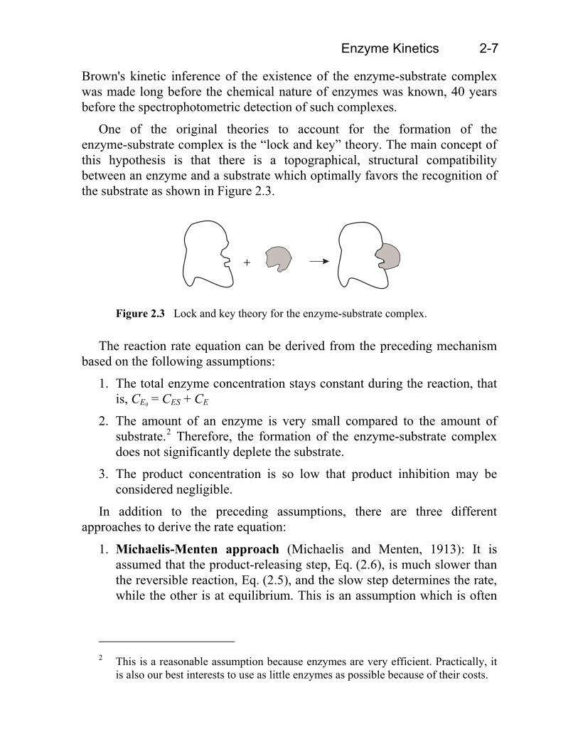
One of the original theories to account for the formation of the enzyme-substrate complex is the “lock and key” theory. The main concept of this hypothesis is that there is a topographical, structural compatibility between an enzyme and a substrate which optimally favors the recognition of the substrate as shown in Figure 2.3.

+

Figure 2.3 Lock and key theory for the enzyme-substrate complex.

The reaction rate equation can be derived from the preceding mechanism based on the following assumptions:

1. The total enzyme concentration stays constant during the reaction, that is, CE0 = CES + CE

2. The amount of an enzyme is very small compared to the amount of substrate.2 Therefore, the formation of the enzyme-substrate complex does not significantly deplete the substrate.

3. The product concentration is so low that product inhibition may be considered negligible.

In addition to the preceding assumptions, there are three different approaches to derive the rate equation:

1. Michaelis-Menten approach (Michaelis and Menten, 1913): It is assumed that the product-releasing step, Eq. (2.6), is much slower than the reversible reaction, Eq. (2.5), and the slow step determines the rate, while the other is at equilibrium. This is an assumption which is often

2 This is a reasonable assumption because enzymes are very efficient. Practically, it

is also our best interests to use as little enzymes as possible because of their costs.

2-8 Enzyme Kinetics

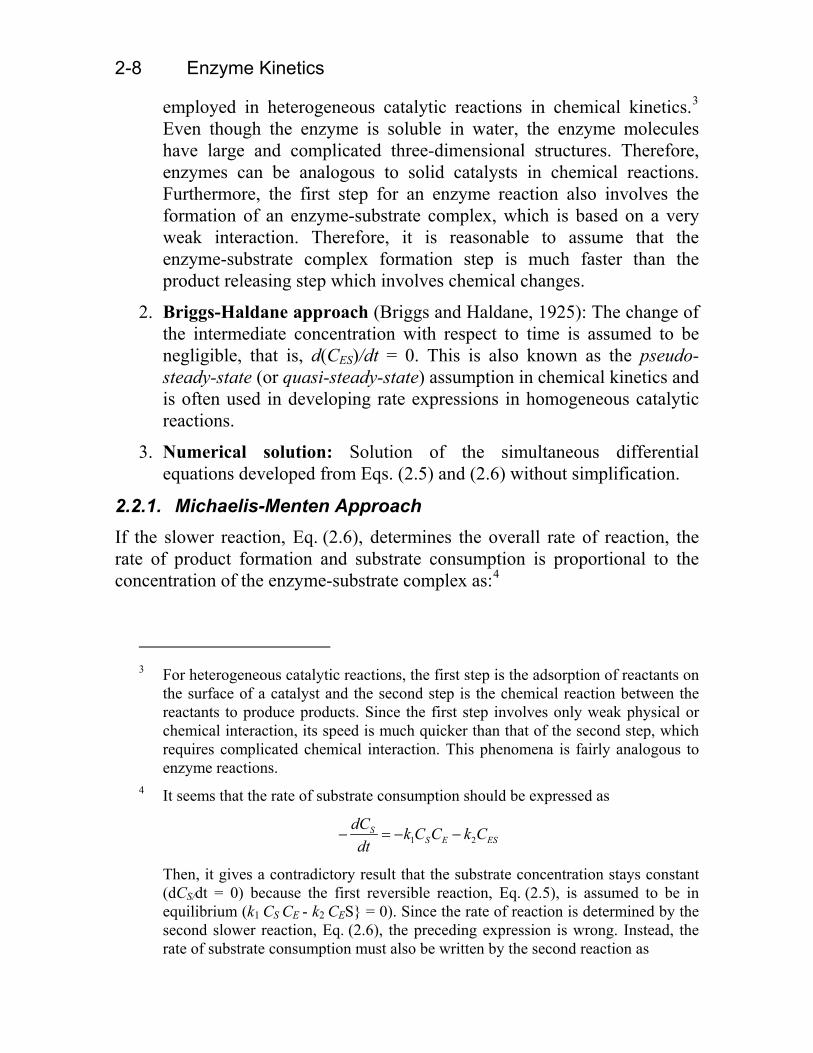
employed in heterogeneous catalytic reactions in chemical kinetics.3 Even though the enzyme is soluble in water, the enzyme molecules have large and complicated three-dimensional structures. Therefore, enzymes can be analogous to solid catalysts in chemical reactions. Furthermore, the first step for an enzyme reaction also involves the formation of an enzyme-substrate complex, which is based on a very weak interaction. Therefore, it is reasonable to assume that the enzyme-substrate complex formation step is much faster than the product releasing step which involves chemical changes.

2. Briggs-Haldane approach (Briggs and Haldane, 1925): The change of the intermediate concentration with respect to time is assumed to be negligible, that is, d(CES)/dt = 0. This is also known as the pseudo-steady-state (or quasi-steady-state) assumption in chemical kinetics and is often used in developing rate expressions in homogeneous catalytic reactions.

3. Numerical solution: Solution of the simultaneous differential equations developed from Eqs. (2.5) and (2.6) without simplification.

2.2.1. Michaelis-Menten Approach If the slower reaction, Eq. (2.6), determines the overall rate of reaction, the rate of product formation and substrate consumption is proportional to the concentration of the enzyme-substrate complex as:4

3 For heterogeneous catalytic reactions, the first step is the adsorption of reactants on

the surface of a catalyst and the second step is the chemical reaction between the reactants to produce products. Since the first step involves only weak physical or chemical interaction, its speed is much quicker than that of the second step, which requires complicated chemical interaction. This phenomena is fairly analogous to enzyme reactions.

4 It seems that the rate of substrate consumption should be expressed as

1 2S

S E ESdC k C C k Cdt

� � �

Then, it gives a contradictory result that the substrate concentration stays constant (dCS/dt = 0) because the first reversible reaction, Eq. (2.5), is assumed to be in equilibrium (k1 CS CE - k2 CES} = 0). Since the rate of reaction is determined by the second slower reaction, Eq. (2.6), the preceding expression is wrong. Instead, the rate of substrate consumption must also be written by the second reaction as

Enzyme Kinetics 2-9

3P S

ESdC dCrdt dt

� k C (2.7)

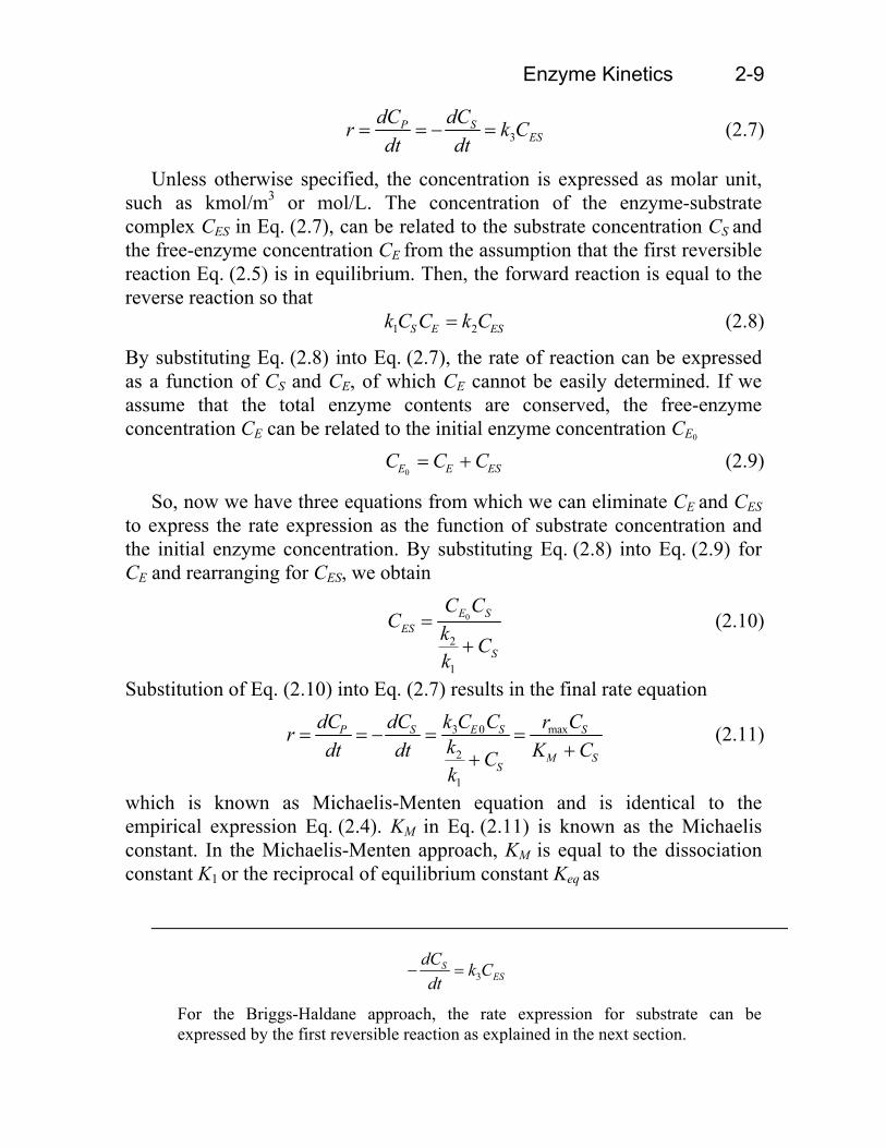
Unless otherwise specified, the concentration is expressed as molar unit, such as kmol/m3 or mol/L. The concentration of the enzyme-substrate complex CES in Eq. (2.7), can be related to the substrate concentration CS and the free-enzyme concentration CE from the assumption that the first reversible reaction Eq. (2.5) is in equilibrium. Then, the forward reaction is equal to the reverse reaction so that 1 2S E ESk C C k C (2.8)

By substituting Eq. (2.8) into Eq. (2.7), the rate of reaction can be expressed as a function of CS and CE, of which CE cannot be easily determined. If we assume that the total enzyme contents are conserved, the free-enzyme concentration CE can be related to the initial enzyme concentration CE0

0E E EC C C S � (2.9)

So, now we have three equations from which we can eliminate CE and CES to express the rate expression as the function of substrate concentration and the initial enzyme concentration. By substituting Eq. (2.8) into Eq. (2.9) for CE and rearranging for CES, we obtain

0

2

1

E SES

S

C CC k C

k

�

(2.10)

Substitution of Eq. (2.10) into Eq. (2.7) results in the final rate equation

3 0 max

2

1

P S E S S

M SS

dC dC k C C r Cr kdt dt K CCk

� ��

(2.11)

which is known as Michaelis-Menten equation and is identical to the empirical expression Eq. (2.4). KM in Eq. (2.11) is known as the Michaelis constant. In the Michaelis-Menten approach, KM is equal to the dissociation constant K1 or the reciprocal of equilibrium constant Keq as

3S

ESdC k Cdt

�

For the Briggs-Haldane approach, the rate expression for substrate can be expressed by the first reversible reaction as explained in the next section.

2-10 Enzyme Kinetics

21

1 e

1S EM

ES

k C CK Kk C

qK

(2.12)

The unit of KM is the same as CS. When KM is equal to CS, r is equal to one half of rmax according to Eq. (2.11). Therefore, the value of KM is equal to the substrate concentration when the reaction rate is half of the maximum rate rmax (see Figure 2.2). KM is an important kinetic parameter because it characterizes the interaction of an enzyme with a given substrate.

Another kinetic parameter in Eq. (2.11) is the maximum reaction rate rmax, which is proportional to the initial enzyme concentration. The main reason for combining two constants k3 and CE0 into one lumped parameter rmax is due to the difficulty of expressing the enzyme concentration in molar unit. To express the enzyme concentration in molar unit, we need to know the molecular weight of enzyme and the exact amount of pure enzyme added.

The constant k3 (also frequently termed kcat) in Eq. (2.11) is also known as turnover number, which is the maximum number of substrate molecules that can be converted per unit time per active site on the enzyme.

When the exact purified quantity of enzyme is not known, it is common to express enzyme concentration as an arbitrarily defined unit based on its catalytic ability. For example, one unit of an enzyme, cellobiose, can be defined as the amount of enzyme required to hydrolyze cellobiose to produce 1 µmol of glucose per minute.

The purity of enzyme solution can be expressed as specific activity as

enzyme activity of product releasedSpecific Activity of protein of protein

mmol mL smg mg

As the enzyme is purified, the specific activity will reach a maximum value at a specified condition (temperature, pH, substrate, enzyme concentration, etc.).

The Michaelis-Menten equation is analogous to the Langmuir isotherm equation

A

A

CK C

T �

(2.13)

where T is the fraction of the solid surface covered by gas molecules and K is the reciprocal of the adsorption equilibrium constant.

2-14 Enzyme Kinetics

3 ESPdC k C

dt (2.14)

1 2 3ES

S E ES ESdC k C C k C k C

dt � � (2.30)

1 2S

S E ESdC k C C k Cdt

� � (2.31)

Eqs. (2.14), (2.30), and (2.31) with Eq. (2.9) can be solved simultaneously without simplification. Since the analytical solution of the preceding simultaneous differential equations are not possible, we need to solve them numerically by using various mathematic softwares such as Mathlab (The Mathworks, Inc., Natick, MA), Mathematica (Wolfram Research, Inc., Champaign, IL), MathCad (MathSoft, Inc., Cambridge, MA), or Polymath (Polymath Software, Willimantic, CT).

It should be noted that this solution procedure requires the knowledge of elementary rate constants, k1, k2, and k3. The elementary rate constants can be measured by the experimental techniques such as pre-steady-state kinetics and relaxation methods (Bailey and Ollis, pp. 111–113, 1986), which are much more complicated compared to the methods to determine KM and rmax. Furthermore, the initial molar concentration of an enzyme should be known, which is also difficult to measure as explained earlier. However, a numerical solution with the elementary rate constants can provide a more precise picture of what is occurring during the enzyme reaction, as illustrated in the following example problem.

––––––––––––––––––––––––––––––––––––––––––––––––––––––––––––––

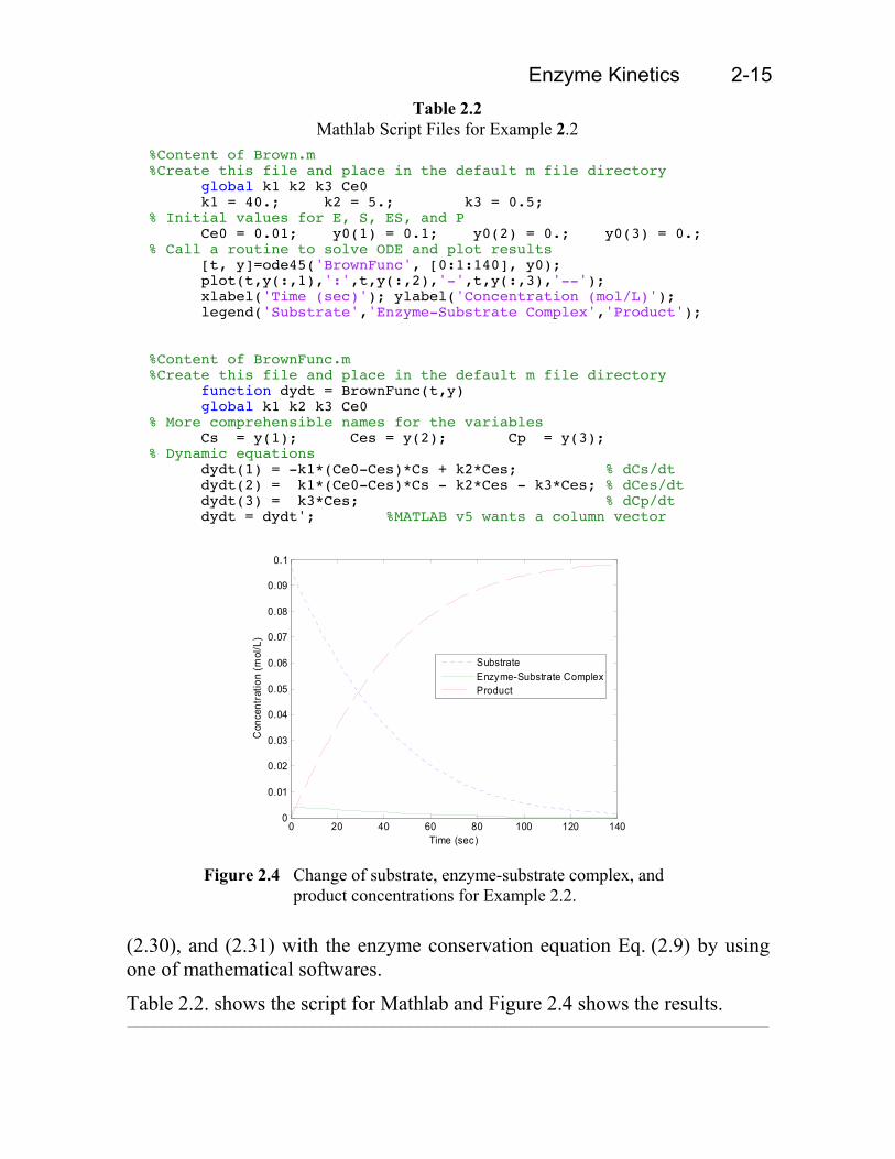
Example 2.2 By employing the computer method, show how the concentrations of substrate, product, and enzyme-substrate complex change with respect to time in a batch reactor for the enzyme reactions described by Eqs. (2.5) and (2.6). The initial substrate and enzyme concentrations are 0.1 and 0.01 mol/L, respectively. The values of the reaction constants are: k1 = 40 L/mols, k2 = 5 s�1, and k3 = 0.5 s�1.

Solution: To determine how the concentrations of the substrate, product, and enzyme-substrate complex are changing with time, we can solve Eqs. (2.14),

Enzyme Kinetics 2-15 Table 2.2

Mathlab Script Files for Example 2.2 %Content of Brown.m %Create this file and place in the default m file directory global k1 k2 k3 Ce0 k1 = 40.; k2 = 5.; k3 = 0.5; % Initial values for E, S, ES, and P Ce0 = 0.01; y0(1) = 0.1; y0(2) = 0.; y0(3) = 0.; % Call a routine to solve ODE and plot results [t, y]=ode45('BrownFunc', [0:1:140], y0); plot(t,y(:,1),':',t,y(:,2),'-',t,y(:,3),'--'); xlabel('Time (sec)'); ylabel('Concentration (mol/L)'); legend('Substrate','Enzyme-Substrate Complex','Product'); %Content of BrownFunc.m %Create this file and place in the default m file directory function dydt = BrownFunc(t,y) global k1 k2 k3 Ce0 % More comprehensible names for the variables Cs = y(1); Ces = y(2); Cp = y(3); % Dynamic equations dydt(1) = -k1*(Ce0-Ces)*Cs + k2*Ces; % dCs/dt dydt(2) = k1*(Ce0-Ces)*Cs - k2*Ces - k3*Ces; % dCes/dt dydt(3) = k3*Ces; % dCp/dt dydt = dydt'; %MATLAB v5 wants a column vector

0 20 40 60 80 100 120 1400

0.01

0.02

0.03

0.04

0.05

0.06

0.07

0.08

0.09

0.1

Time (sec)

Con

cent

ratio

n (m

ol/L

)

SubstrateEnzyme-Substrate ComplexProduct

Figure 2.4 Change of substrate, enzyme-substrate complex, and product concentrations for Example 2.2.

(2.30), and (2.31) with the enzyme conservation equation Eq. (2.9) by using one of mathematical softwares.

Table 2.2. shows the script for Mathlab and Figure 2.4 shows the results. –––––––––––––––––––––––––––––––––––––––––––––––––––––––––––––––––––––––––

2-16 Enzyme Kinetics

2.3. Evaluation of Kinetic Parameters In order to estimate the values of the kinetic parameters, we need to make a series of batch runs with different levels of substrate concentration. Then the initial reaction rate can be calculated as a function of initial substrate concentrations. The results can be plotted graphically so that the validity of the kinetic model can be tested and the values of the kinetic parameters can be estimated.

The most straightforward way is to plot r against CS as shown in Figure 2.2. The asymptote for r will be rmax and KM is equal to CS when r = 0.5 rmax. However, this is an unsatisfactory plot in estimating rmax and KM because it is difficult to estimate asymptotes accurately and also difficult to test the validity of the kinetic model. Therefore, the Michaelis-Menten equation is usually rearranged so that the results can be plotted as a straight line. Some of the better known methods are presented here. The Michaelis-Menten equation, Eq. (2.11), can be rearranged to be expressed in linear form. This can be achieved in three way:

max max

S MC K Cr r r � S (2.32)

max max

1 1 1M

s

Kr r r C � (2.33)

max MS

rr r KC

� (2.34)

An equation of the form of Eq. (2.32) was given by Langmuir (Carberry, 1976) for the treatment of data from the adsorption of gas on a solid surface. If the Michaelis-Menten equation is applicable, the Langmuir plot will result in a straight line, and the slope will be equal to 1/rmax. The intercept will be

maxMK r , as shown in Figure 2.5.

Similarly, the plot of 1/r versus 1/CS will result in a straight line according to Eq. (2.33), and the slope will be equal to maxMK r . The intercept will be 1/rmax, as shown in Figure 2.6. This plot is known as Lineweaver-Burk plot (Lineweaver and Burk, 1934).

The plot of r versus r/CS will result in a straight line with a slope of –KM and an intercept of rmax, as shown in Figure 2.7. This plot is known as the Eadie-Hofstee plot (Eadie, 1942; Hofstee, 1952).

Enzyme Kinetics 2-17

0 20 40 60 80

5

10

15

20

CS

r

CS

KM

rmax

1rmax

Figure 2.5 The Langmuir plot (KM = 10, rmax = 5).

0-0.05 0.05 0.10 0.15

0.2

0.4

0.6

1r

1CS

1rmax

KM

rmax

Figure 2.6 The Lineweaver-Burk plot (KM = 10, rmax = 5).

The Lineweaver-Burk plot is more often employed than the other two plots because it shows the relationship between the independent variable CS and the dependent variable r. However, 1/r approaches infinity as CS decreases, which gives undue weight to inaccurate measurements made at low substrate concentrations, and insufficient weight to the more accurate measurements at high substrate concentrations. This is illustrated in Figure 2.6. The points on the line in the figure represent seven equally spaced substrate concentrations. The space between the points in Figure 2.6 increases with the decrease of CS.

On the other hand, the Eadie-Hofstee plot gives slightly better weighting of the data than the Lineweaver-Burk plot (see Figure 2.7). A disadvantage of this plot is that the rate of reaction r appears in both coordinates while it is usually regarded as a dependent variable. Based on the data distribution, the Langmuir plot (CS /r versus CS) is the most satisfactory of the three, since the points are equally spaced (see Figure 2.5).

2-34 Enzyme Kinetics

2.7. Experiment: Enzyme Kinetics

Objectives:

The objectives of this experiment are:

1. To give students an experience with enzyme reactions and assay procedures

2. To determine the Michaelis-Menten kinetic parameters based on initial-rate reactions in a series of batch runs

3. To simulate batch and continuous runs based on the kinetic parameters obtained

Materials:

1. Spectrophotometer

2. 10g/L glucose standard solution

3. Glucose assay kit (No. 16-UV, Sigma Chemical Co., St. Louis, MO)

4. Cellobiose

5. Cellobiase enzyme (Novozym 188, Novo Nordisk Bioindustrials Inc., Danbury, CT) or other cellulase enzyme

6. 0.05M (mol/L) sodium acetate buffer (pH 5)

7. 600 mL glass tempering beaker (jacketed) (Cole-Parmer Instrument Co., Chicago, IL) with a magnetic stirrer

8. Water bath to control the temperature of the jacketed vessel

Calibration Curve for Glucose Assay:

1. Prepare glucose solutions of 0, 0.5, 1.0, 3.0, 5.0 and 7.0g/L by diluting 10g/L glucose standard solution.

2. Using these standards as samples, follow the assay procedure described in the brochure provided by Sigma Chemical Co.

3. Plot the resulting absorbances versus their corresponding glucose concentrations and draw a smooth curve through the points.

Enzyme Kinetics 2-35

Experiment Procedures:

1. Prepare a 0.02M cellobiose solution by dissolving 3.42 g in 500 mL of 0.05M NaAc buffer (pH 5).

2. Dilute the cellobiase-enzyme solution so that it contains approximately 20 units of enzyme per mL of solution. One unit of cellobiase is defined as the amount of enzyme needed to produce 1 µ-mol of glucose per min.

3. Turn on the bath circulator, making sure that the temperature is set at 50qC.

4. Pour 100 mL of cellobiose solution with a certain concentration (20, 10, 5, 2, or 1mM) into the reactor, turn on the stirrer, and wait until the solution reaches 50qC. Initiate the enzyme reaction by adding 1 mL of cellobiase solution to the reaction mixture and start to time.

5. Take a 1 mL sample from the reactor after 5- and 10-minutes and measure the glucose concentration in the sample.

Data Analysis:

1. Calculate the initial rate of reaction based on the 5 and 10 minute data.

2. Determine the Michaelis-Menten kinetic parameters as described in this chapter.

3. Simulate the change of the substrate and product concentrations for batch and continuous reactors based on the kinetic parameters obtained. Compare one batch run with the simulated results. For this run, take samples every 5 to 10 minutes for 1 to 2 hours.

––––––––––––––––––––––––––––––––––––––––––––––––––––––––––––––

2.8. Nomenclature A0 constant called frequency factor in Arrhenius equation, dimensionless C concentration, kmol/m3 D dilution rate, s-1 E activation energy (kcal/kmol) F flow rate, m3/s k rate constant KM Michaelis constant, kmol/m3

2-36 Enzyme Kinetics

K dissociation constant Keq equilibrium constant R gas constant (kcal/kmol qK) r rate of reaction per unit volume, kmol/m3s rmax maximum rate of reaction per unit volume, kmol/m3s T temperature qK t time, s V working volume of reactor, m3 W residence time, s

Subscript E enzyme EI enzyme-inhibitor complex ES enzyme-substrate complex I inhibitor P product S substrate

––––––––––––––––––––––––––––––––––––––––––––––––––––––––––––––

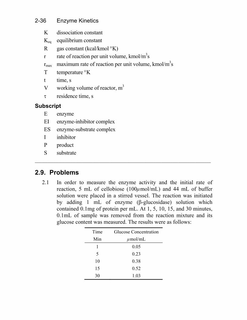
2.9. Problems 2.1 In order to measure the enzyme activity and the initial rate of

reaction, 5 mL of cellobiose (100µmol/mL) and 44 mL of buffer solution were placed in a stirred vessel. The reaction was initiated by adding 1 mL of enzyme (β-glucosidase) solution which contained 0.1mg of protein per mL. At 1, 5, 10, 15, and 30 minutes, 0.1mL of sample was removed from the reaction mixture and its glucose content was measured. The results were as follows:

Time Glucose Concentration Min µmol/mL

1 0.05 5 0.23 10 0.38 15 0.52 30 1.03

Enzyme Kinetics 2-45

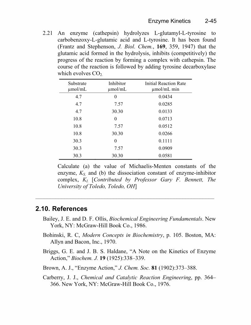
2.21 An enzyme (cathepsin) hydrolyzes L-glutamyl-L-tyrosine to carbobenzoxy-L-glutamic acid and L-tyrosine. It has been found (Frantz and Stephenson, J. Biol. Chem., 169, 359, 1947) that the glutamic acid formed in the hydrolysis, inhibits (competitively) the progress of the reaction by forming a complex with cathepsin. The course of the reaction is followed by adding tyrosine decarboxylase which evolves CO2.

Substrate µmol/mL

Inhibitor µmol/mL

Initial Reaction Rate µmol/mL min

4.7 0 0.0434 4.7 7.57 0.0285 4.7 30.30 0.0133 10.8 0 0.0713 10.8 7.57 0.0512 10.8 30.30 0.0266 30.3 0 0.1111 30.3 7.57 0.0909 30.3 30.30 0.0581

Calculate (a) the value of Michaelis-Menten constants of the enzyme, KS, and (b) the dissociation constant of enzyme-inhibitor complex, KI. [Contributed by Professor Gary F. Bennett, The University of Toledo, Toledo, OH]

––––––––––––––––––––––––––––––––––––––––––––––––––––––––––––––

2.10. References Bailey, J. E. and D. F. Ollis, Biochemical Engineering Fundamentals. New

York, NY: McGraw-Hill Book Co., 1986.

Bohinski, R. C, Modern Concepts in Biochemistry, p. 105. Boston, MA: Allyn and Bacon, Inc., 1970.

Briggs, G. E. and J. B. S. Haldane, “A Note on the Kinetics of Enzyme Action,” Biochem. J. 19 (1925):338–339.

Brown, A. J., “Enzyme Action,” J. Chem. Soc. 81 (1902):373–388.

Carberry, J. J., Chemical and Catalytic Reaction Engineering, pp. 364–366. New York, NY: McGraw-Hill Book Co., 1976.