Bio-inspired Microvascular Exchangers Employing

Circular Packing – Synthetic Rete Mirabile

Du T. Nguyen‡, Maya Kleiman†, Richard Truong†, and Aaron P. Esser-Kahn*,†

†Department of Chemistry, University of California, Irvine, Irvine CA, 92697, United States

‡Department of Physics and Astronomy, University of California, Irvine, Irvine CA, 92697,

United States

Supporting Information

Table of Contents

1. Close Packing Design2. Exchange Unit Fabrication3. COMSOL Model: Mass and Heat Transport4. CO2 MEA Reaction Mechanism5. Mass Transfer Experiment6. Fluorescent Temperature Measurement Probe7. Heat Transfer Temperature Probe Calibration8. Heat Transfer Experimental Details9. Heat Transfer Calculations10. Nusselt Numbers11. Transfer Coefficient Correlations

1. Close Packing Design

For these circular patterns, there are only nine possible radii ratios that lead to close packed configurations in a binary system (Fig. S1).[1] Each close packed pattern contains an ideal ratio between circle diameters to remain close packed. Of the nine patterns, two have been identified in nature: the “Hexagonal“ and “Squarer“ patterns. We chose two other patterns to examine due to their similarities to the ones found in nature: the “Dodecagonal“ and “Double Squarer“. The “Dodecagonal“ and “Hexagonal“ patterns both have equilateral triangular unit cells while the

Electronic Supplementary Material (ESI) for Materials Horizons.This journal is © The Royal Society of Chemistry 2014

“Double Squarer“ and “Squarer“ patterns are the only patterns with quadrilateral unit cells. The other unit patterns were not examined in this report due to unit cell shape (a,b,e), asymmetric unit cell (c), or lack of available microfibers for fabrication (i).

Figure S1. Close packing of discs of two sizes. The nine possible close packing disc radii ratios are displayed. The “r” values indicate the ratio between the two radii in each pattern.

In designing the exchange unit patterns, primary requirement was to maintain a 50 µm minimum separation. This requirement was enforced as the fabrication plates are unable to have smaller separations. The available microchannel sizes were 100, 200, 300, and 500 µm diameters, which drove the modification of the packing pattern geometries (Table S1, Fig. S2). The hexagonal

pattern contains the greatest deviation from the ideal parameters due to its use in our previous microvascular mass transport studies. To obtain the modified parameters, the ideal parameters were scaled to be ~20% larger than available fiber diameters. Then 50 µm was subtracted from one set of channel diameters. Finally, the results were rounded to the nearest available channel diameters.

Table S1. Packing pattern geometries. Ideal channel diameters represent the closest possible packing arrangement using the pattern. For practical fabrication, channel diameters were adjusted to compensate for membrane thicknesses and available channel sizes.

Ideal Channel Diameter (µm)

Adjusted Channel Diameter (µm)

Measured Channel Diameter (µm)

Packing Pattern

Large Small Large Small Large Small

Interchannel Distance (µm)

Packing Density (%)

Modified Hexagonal 350 54 300 200 318 ± 5 207 ± 9 52 ± 6 57

Dodecagonal 500 175 500 100 503 ± 8 99 ± 3 51 ± 8 61

Squarer 350 145 300 200 306 ± 5 205 ±4 52 ± 4 57

Double Squarer 300 84 300 100 312 ± 5 100 ± 6 53 ± 2 55

Figure S2. Plate pattern designs. Plate designs were constructed in AutoCAD. Additional space was added to the hole sizes to allow for easier threading of sacrificial fibers. (A) Hexagonal. (B) Squarer. (C) Dodecagonal. (D) Double Squarer.

2. Exchange Unit Fabrication

Fibers were treated according to the Vaporization of Sacrificial Components (VaSC) technique with some modifications.1 Briefly, tin oxalate is incorporated into PLA fibers through entrapment within the swollen surface of the fibers. The incorporation of tin oxalate lowers the depolymerization temperature of PLA down to 200 °C. When placed under heat and vacuum, the solid PLA polymer depolymerizes into gaseous monomers which can be evacuated when placed within a template. 800 mL of treatment solution was used (400 mL deionized water, 400 mL TFE, 50 g tin oxalate, 20 g disperbyk-130, 0.5 g malachite green). Fibers were wound around a custom spindle and placed in the solution. The spindle comprised of six steel rods affixed around a central core with a mixer at the bottom (Fig. S3). The solution with fibers was agitated with a digital mixer (IKA RW20) at 250 RPM for 48 h at 25° C.

Figure S3. Custom spindle for fibers to wrap around. The spindel is built to ensure proper mixing of the catalyzing solution while reducing surface contact with the fibers.

Polydimethylsiloxane (PDMS) was created using mixtures of the Slygard 184 silicone elastomer base and curing agent with a 10:1 ratio between base and curing agent inside paper cups. The mixtures were then degassed using a rough vacuum pump and glass bell jar for 15 minutes.

Treated fibers were patterned using laser micromachined brass plates manufactured by Hodge Harland at the University of Illinois at Urbana-Champaign (Fig. S4). Fibers were strung through matching holes on a pair of plates which were then screwed onto a delrin mold box with dimensions of 25×25×25 mm. The fibers were tensioned until taut on a custom board with pairs of guitar tuning pegs on either side (Fig. S5, S6). The degassed PDMS mixtures was poured into the mold and heated at 65°C for 1 h using a Breville Smart Oven to complete the polymerization reaction.

Figure S4. Laser-etched micromachined brass plates. Fibers are strung through the holes in the end caps, providing the desired pattern.

Figure S5. Example custom molding board. Guitar tuners on either side provide tensioning for fibers.

Figure S6. Assembled molding setup. Fibers are tensioned through the brass end caps using the tuning board. Metal rods in the board act as pullys to help tuning pegs along the side of the board to tension the fibers.

The units were then removed from the first mold and placed into a second mold box with dimensions of 25×25×50 mm. The fibers were separated and threaded through PDMS end-caps which were screwed onto the mold box. Syringe needles (B-D PrecisionGlide 18G1 Needle) were inserted through the PDMS end caps and fibers were threaded through the needles. The needles were removed leaving the fibers in the end caps. The end caps were screwed onto the larger mold box and fibers were pulled taut by hand. A second mold of PDMS was then cast again at 65°C for 1 h (Fig. S7). Longer samples were created using a 25×25×50 mm box as the first mold and 25×25×75 mm box as the second mold.

Figure S7. Exchange unit after second molding. Fibers are separated into a larger pattern for easier loading of channels.

The vascular preforms were removed from the second mold. The remaining fibers extending out of the PDMS were then cut from the edges of the molded shape. The vascular preforms were placed into a sealed vacuum oven (JEIO Tech Vacuum Oven Model OV-11/12) and subjected to a vacuum of 10 torr and heated to 210 °C for 48 h.

3. COMSOL Model: Mass and Heat Transport

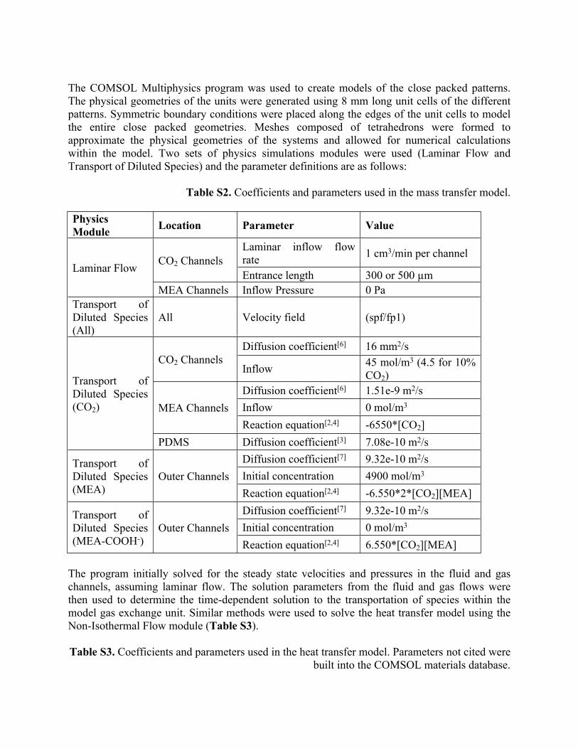
The COMSOL Multiphysics program was used to create models of the close packed patterns. The physical geometries of the units were generated using 8 mm long unit cells of the different patterns. Symmetric boundary conditions were placed along the edges of the unit cells to model the entire close packed geometries. Meshes composed of tetrahedrons were formed to approximate the physical geometries of the systems and allowed for numerical calculations within the model. Two sets of physics simulations modules were used (Laminar Flow and Transport of Diluted Species) and the parameter definitions are as follows:

Table S2. Coefficients and parameters used in the mass transfer model.

Physics Module Location Parameter Value

Laminar inflow flow rate 1 cm3/min per channelCO2 ChannelsEntrance length 300 or 500 µmLaminar Flow

MEA Channels Inflow Pressure 0 PaTransport of Diluted Species (All)

All Velocity field (spf/fp1)

Diffusion coefficient[6] 16 mm2/sCO2 Channels

Inflow 45 mol/m3 (4.5 for 10% CO2)

Diffusion coefficient[6] 1.51e-9 m2/sInflow 0 mol/m3MEA ChannelsReaction equation[2,4] -6550*[CO2]

Transport of Diluted Species (CO2)

PDMS Diffusion coefficient[3] 7.08e-10 m2/sDiffusion coefficient[7] 9.32e-10 m2/sInitial concentration 4900 mol/m3

Transport of Diluted Species (MEA)

Outer ChannelsReaction equation[2,4] -6.550*2*[CO2][MEA]Diffusion coefficient[7] 9.32e-10 m2/sInitial concentration 0 mol/m3

Transport of Diluted Species (MEA-COOH-)

Outer ChannelsReaction equation[2,4] 6.550*[CO2][MEA]

The program initially solved for the steady state velocities and pressures in the fluid and gas channels, assuming laminar flow. The solution parameters from the fluid and gas flows were then used to determine the time-dependent solution to the transportation of species within the model gas exchange unit. Similar methods were used to solve the heat transfer model using the Non-Isothermal Flow module (Table S3).

Table S3. Coefficients and parameters used in the heat transfer model. Parameters not cited were built into the COMSOL materials database.

Physics Module Location Parameter Value

All Velocity field (spf/fp1)

Density 838.466+1.401*T-.003011*T2+3.718E-7*T3 kg/m3

Heat Capacity at Constant Pressure

12010-80.41*T+.3099*T2-5.382E-4*T3+3.623E-7*T4 J/(kg*K)

Thermal Conductivity

-0.8691+0.008949*T-1.564E-5*T2+7.975E-9*T3 W/(m*K)Fluid

Channels

Dynamic Viscosity

1.3799566804-0.021224019151*T+1.3604562827E-4*T2-4.645090319E-7*T3+8.9042735735E-10*T4-9.0790692686E-13*T5+3.8457331488E-16*T6 Pa*s

Laminar inflow flow rate 0.2 cm3/min per channel

Entrance length 300 or 500 µmHot Channels

Temperature 45 °CLaminar inflow flow rate

0.1 cm3/min per channel (Countercurrent Direction)

Entrance length 200 or 100 µmColder Channels

Temperature 25 °C

Density[5] 970 kg/m3

Heat Capacity at Constant Pressure[5]

1460 J/(kg*K)

Non-Isothermal Flow

PDMS

Thermal Conductivity[5] 0.15 W/(m*K)

4. CO2 MEA Reaction Mechanism

The reaction between CO2 and MEA is a two-step reaction mechanism which occurs through a zwitterion intermediate (Figure S8).[4-6] MEA and CO2 react to form a zwitterion intermediate as the rate-determining step. Following this zwitterion formation, an acid-base reaction occurs between the zwitterion and another MEA to form carbamate.

Figure S8. CO2-MEA reaction mechanism. Heating the solution drives the reverse reaction, releasing CO2.

5. Mass Transfer Experiment

1 mg of 5-(and-6)-carboxynaphthofluorescein diacetate dye was added to 6 mL of 30% monoethanolamine (MEA) to create the dyed solution. Each close packed structure was separated into fluid and gas channels, with the smaller channels corresponding to the fluid and the larger channels corresponding to the gas channels. The dyed MEA was loaded into the central fluid channels which were completely surrounded by gas channels. CO2 was flowed through the gas channels at a flow rate of 1 mL/min per gas channel using a mass flow controller (SmartTrak 50 Mass Flow Controller). Time lapsed images were taken with a Zeiss Axio Observer.A1 Microscope using a 2.5 X objective at intervals of 6 seconds for 5 minutes (Fig. S9). The fluorescence intensity was set to the minimum possible intensity. The microscope shutter was manually operated to prevent photo-bleaching of the dye.

Figure S9. Mass transfer experimental schematic. The flow of CO2 is controlled by a mass flow controller to maintain a constant flow rate. A pH sensitive fluorescent dye monitors the transfer of CO2 from one set of channels to another under the observation of a fluorescent microscope.

6. Fluorescent Temperature Measurement Probe

Rhodamine has previously been used to measure the temperature within microfluidic channels. However, these dyes can diffuse into the PDMS membrane and lower the accuracy of the temperature measurements. A two phase technique was used to optically measure the temperature profiles within the close packed exchangers. The pH sensitivity of fluorescein was coupled to the temperature sensitivity of Tris-HCL buffer. The relationship between intensity and pH is nonlinear for fluorescein within a larger range of pH, but within the values of 6-7, it is linear. This phenomena is useful as the relationship between pH and temperature for Tris-HCl is approximately linear within the pH range of 6-7 and a temperature range of 20-80 °C.

7. Heat Transfer Temperature Probe Calibration

A 250 mL solution of 10 µM Fluorescein in 10 mM Tris-HCl adjusted to a pH of 7.1 at 22 °C was prepared as the temperature probe. A 2.5 cm long, 300 µm diameter microchannel was fabricated with a thermistor element (Omega 5500 Series Glass Encapsulated Thermistor) embedded in contact with the microchannel in PDMS. A 7.5 cm long, 500 µm diameter microchannel was fabricated with a resistive heating wire coiled around the length of the microchannel to act as the heating element (Omega, Resistance Heating Wire, Nickel-Chromium Alloy, 80% Nickel/ 20% Chromium). A peristaltic pump (Buchler Polystaltic Pump) was used to flow the temperature probe solution through the heater and temperature sensing element at varying flow rates. The varying flow rates allowed for the temperature at the sensing element to change, while the change in intensity was measured using a fluorescent microscope (Fig S10). Time lapsed images were taken using a Zeiss Axio Observer.A1 Microscope. A 5 X objective was employed and images were aquired at intervals of 30 seconds for 20 minutes were taken for each temperature point. Baseline intensity measurements were also taken as the reference point for the intensity changes.

Figure S10. Heat transfer temperature probe calibration. (A) Calibration schematic. The temperature probe flows continuously through a microchannel after being heated under different flow rates. The temperature is measured with a thermistor element and the intensity of the probe is measured with a fluorescent microscope. (B) Calibration results. A linear relationship between the normalized intensity and temperature was found within the temperature range between 75 and 25 °C.

8. Heat Transfer Experimental Details

A 250 mL solution of 10 µM Fluorescein in 10 mM Tris-HCl adjusted to a pH of 7.1 at 22 °C was prepared as the temperature probe. All liquid solutions and exchangers were degassed under vacuum prior to conducting the experiments. The exchangers were separated into warm and colder channels, with the small channels corresponding to the colder set and the larger channels corresponding to the warmer set. The temperature probing solution flowed through the warm and colder channels in separate runs to measure the temperature profiles of the exchangers. Water flowed through the opposite channel sets. Peristaltic pumps (Buchler Polystaltic Pump) were used to flow the fluids through the channels. A water bath was used to regulate the temperature of the fluid reservoirs. A syringe heating jacket (Syringe Heater, Pump Systems Inc.) surrounded a stainless steel pipe (1/4 Pipe Size X 3” Length) to heat the fluid entering the warm channels (Fig. S11). Time lapsed images were taken with a Zeiss Axio Observer.A1 Microscope using a 2.5 X objective at intervals of 1 minute for 2 hours were taken to ensure that steady state temperature gradients were reached. The fluorescence intensity was set to the minimum possible intensity. The first 30 minutes of each run began with no heating to obtain a baseline intensity value for the room temperature. After the first 30 minutes, the heating jacket was turned on to a set point of 95 °C. While heat was lost between the heater and exchanger, the temperature profile provided by the temperature probe solution allowed for the precise measurement of the inlet temperatures.

Figure S11. Heat transfer experimental schematic. The flows of the hot and cool fluids are controlled by peristaltic pumps. The fluorescent probe flows through either sets of channels to measure the temperature profile in both.

9. Heat Transfer Calculations

The heat transfer coefficients were calculated based on the temperature gradient across the length of the channels using the log mean temperature differences and channel geometries.

ΔTm = Log mean temperature difference (K)THin = Hot channel inlet temperature (K)THout = Hot channel outlet temperature (K)TCin = Colder channel inlet temperature (K)TCout = Colder channel outlet temperature (K)Q = Heat transferred (W)ρ = Fluid density (g/m3)Cp = Fluid heat capacity at constant pressure (J/g*K)V = Volumetric fluid flow rate (m3/s)q’’ = Heat flux (W/m2)A = Channel surface area (m2)h = Heat transfer coefficient (W/m2*K)Nu = Nusselt numberDh = Channel diameter (m)k = thermal conductivity (W/m*K)

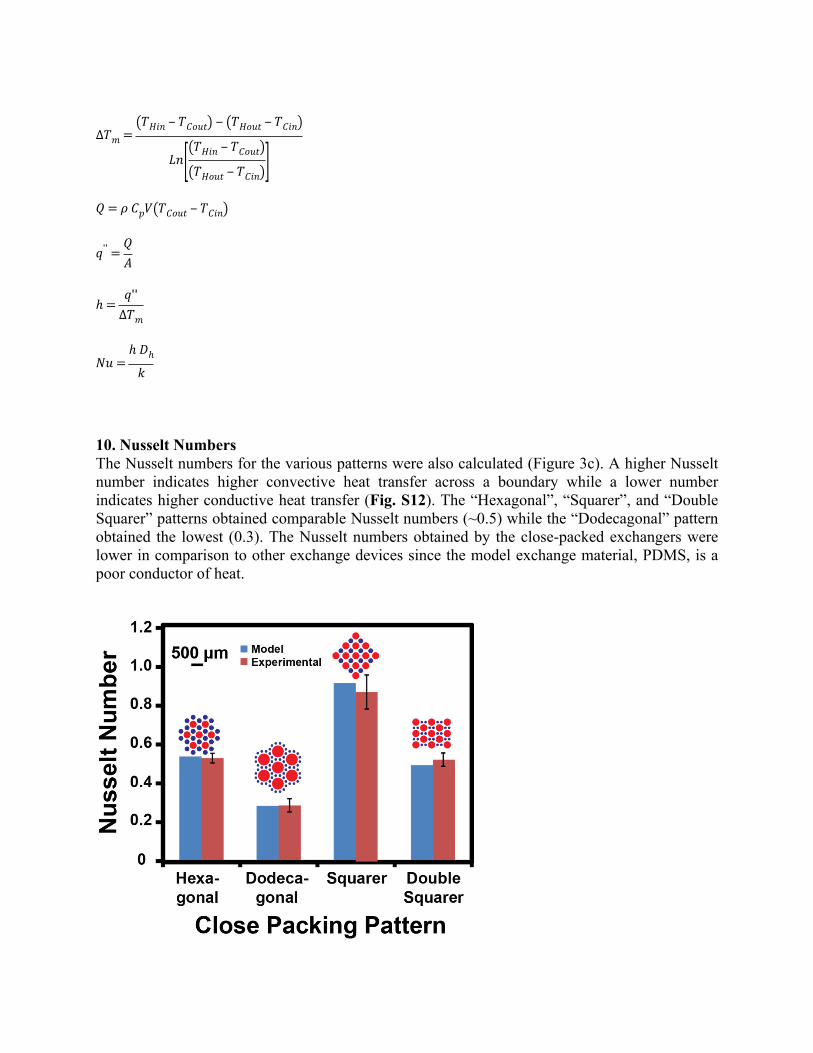
∆𝑇𝑚 =(𝑇𝐻𝑖𝑛 ‒ 𝑇𝐶𝑜𝑢𝑡) ‒ (𝑇𝐻𝑜𝑢𝑡 ‒ 𝑇𝐶𝑖𝑛)

𝐿𝑛[(𝑇𝐻𝑖𝑛 ‒ 𝑇𝐶𝑜𝑢𝑡)(𝑇𝐻𝑜𝑢𝑡 ‒ 𝑇𝐶𝑖𝑛)]

𝑄 = 𝜌 𝐶𝑝𝑉(𝑇𝐶𝑜𝑢𝑡 ‒ 𝑇𝐶𝑖𝑛)

𝑞'' =𝑄𝐴

ℎ =𝑞''

∆𝑇𝑚

𝑁𝑢 =ℎ 𝐷ℎ

𝑘

10. Nusselt NumbersThe Nusselt numbers for the various patterns were also calculated (Figure 3c). A higher Nusselt number indicates higher convective heat transfer across a boundary while a lower number indicates higher conductive heat transfer (Fig. S12). The “Hexagonal”, “Squarer”, and “Double Squarer” patterns obtained comparable Nusselt numbers (~0.5) while the “Dodecagonal” pattern obtained the lowest (0.3). The Nusselt numbers obtained by the close-packed exchangers were lower in comparison to other exchange devices since the model exchange material, PDMS, is a poor conductor of heat.

Figure S12. Nusselt Numbers. The “Hexagonal”, “Squarer”, and “Double Squarer” patterns obtain similar Nusselt numbers while the “Dodecagonal” pattern obtains the lowest. The largest discrepancy between model and experimental values is found in the “Squarer” pattern.

11. Transfer Coefficient Correlations

The distances between the smaller and larger sets of channels were found for each close packed pattern. The distance was calculated from the edge of the smaller channel to the nearest edge of one of the larger channels (Fig. S13). This distance was calculated over the entire arclength of the small channel and used to find the root mean square distance (RMS). Correlations between the RMS distance and the transfer coefficients were found.

Figure S13. Mean distance correlation. (A) Distance calculation. Periodic behavior in determining the nearest channel distances is found. The “Hexagonal” pattern obtains the largest average nearest channel distance while the “Double Squarer” obtains the lowest. (B) Mass transfer correlations. A strong correlation between mass transfer coefficients and root mean square (RMS) distances is found. (C) Heat transfer correlations.

Further investigation into the correlations was performed using the COMSOL models (Figure S14). When the RMS distances were normalized to 61.9 µm (Double Squarer distance), the transfer coefficients maintained similar differences. Next, we examined the effects of normalizing the channel ratios to use 100 µm and 300 µm channel sizes, with normalized RMS distances. Last, we investigated an alternative pattern geometry set where the patterns were normalized to have the same minimum channel size (100 µm), RMS distance (61.9 µm), and larger channel size that matched with the ideal pattern ratio. It should be noted that these other patterns were not currently possible to fabricate due to low minimum inter-channel distances or unavailable fiber sizes. The ideal pattern ratios, normalized minimum channel size, and normalized RMS distances resulted in the “Squarer” pattern obtaining the highest transfer coefficients.

Figure S14. Transfer coefficients. (A) Mass Transfer Coefficients. (B) Heat Transfer Coefficients. Fabricated patterns were limited by fabrication. Thicknesses were normalized to 61.9 µm RMS distance between channels. Normalized ratios used 100 µm channels as the smaller channels, 300 µm channels as the larger ones, and maintained normalized RMS distances. Alternatively, ideal ratios between small and large channels were modeled, using 100 µm channels as the smaller ones and maintained normalized RMS distances.

Last, the transfer coefficients were examined using channel diameters and membrane thicknesses resembling biologically scaled systems. Membrane thicknesses were set to a minimum of ~1 µm (normalized to 3.8 µm RMS thickness). Minimum channel sizes were set to 5 µm and channel ratios were idealized. Flow rates were decreased by a factor of 100 for mass transfer models. Model lengths were reduced from 8000 µm to 800 µm. Transfer coefficients increased for all patterns.Trends remained consistant for both mass and heat transfer coefficients, but less pronounced for the mass transfer coefficients.

Figure S15. Biological scale transfer coefficients. Transfer coefficients were calculated for systems using biological sized channels and membrane thicknesses. 5 µm minimum diameter channels were used with ~1 µm minimum membrane thickness (normalized to 3.8 µm RMS distance) and ideal channel ratios.

References[1] T. Kennedy, Discrete Comput. Geom., 2005, 35, 255–267[2] P. V. Danckwerts, Chem. Eng. Sci. 1979, 34, 443–446.[3] T. C. Merkel, V. I. Bondar, K. Nagai, B. D. Freeman, I. Pinnau, J. Polym. Sci. Part B

Polym. Phys. 2000, 38, 415–434.[4] J. M. Plaza, D. V. Wagener, G. T. Rochelle, Energy Procedia 2009, 1, 1171–1178.[5] J. E. Mark, Polymer Data Handbook, Oxford University Press, Oxford; New York, 2009.[6] W. M. Haynes, D. R. Lide, Bruno, CRC Handbook of Chemistry and Physics: a Ready

Reference Book of Chemical and Physical Data, CRC, Boca Raton, 2012.[7] E. D. Snijder, M. J. M. te Riele, G. F. Versteeg, W. P. M. van Swaaij, J. Chem. Eng. Data

1993, 38, 475–480.