��������������� �������������������������! � "�#���$!�%$'&!(*),+%&�-.-*/.0c1 &�-�-*/32��#�'45�6�37��!.8��69:���;����<��#�� %=�>�� !$.?;�. A@�����BDCE������F.�!@%���6��8G�#�IH5=�KJ���@"=�6�A����8� �B

Binomial Filters

MATTHEW AUBURYu91mpa@ecs.ox.ac.uk

Programming Research Group, Oxford University ComputingLaboratory, Wolfson Building, Parks Road, Oxford, England OX1 3QD

WAYNE LUKw.luk@doc.ic.ac.uk

Department of Computing, Imperial College180 Queen’s Gate, London, England SW7 2BZ

Received November 15, 1994. Revised July 24, 1995.

Abstract. Binomial filters are simple and efficient structures based on the binomial coefficients for implementingGaussian filtering. They do not require multipliers and can therefore be implemented efficiently in programmablehardware. There are many possible variations of the basic binomial filter structure, and they provide a wide rangeof space-time trade-offs; a number of these designs have been captured in a parametrised form and their featuresare compared. This technique can be used for multi-dimensional filtering, provided that the filter is separable.The numerical performance of binomial filters, and their implementation using field-programmable devices for animage processing application, are also discussed.

Keywords: Gaussian filters, binomial filters, parametrised design, field-programmable devices.

1. Introduction

Gaussian filtering is probably the most common formof linear filtering. To overcome the problem of choos-ing filter coefficients against a set of conflicting con-straints, we review an approximation of the Gaussianbased on the binomial coefficients which results in asimple, accurate and flexible architecture. This de-sign, called a binomial filter, does not require mul-tiplications, thus allowing large filters to be easilyimplemented in current programmable hardware tech-nologies, such as Field Programmable Gate Arrays(FPGAs). Moreover, its regular structure facilitatesimplementation in custom VLSI, and transformations[1],[2],[3] can be applied to produce systolic versionswith high performance. It is feasible that such filterscan be implemented alongside other hardware, such asprogrammable DSP chips, at little additional cost.

It is well known that, where applicable, sepa-rating a multi-dimensional filter into a cascade ofone-dimensional filters significantly reduces the num-ber of computations required to implement the filter[4],[5],[6]. In our case, given that L is the size of thefilter and M is the number of dimensions of convolu-

tion, the use of separated binomial methods results ina reduction from LON multiplications and LPNRQTS addi-tions per data point required by conventional methodsto M5UVLWQXS�Y additions and no multiplications. Thisadvantage enables both software and hardware imple-mentations to gain up to two orders of magnitude im-provement in speed over conventional methods.

Some of the basic ideas behind the binomial fil-ter are well known and have been discussed by otherresearchers. For instance, Canny ([6], p. 77) men-tioned the binomial approximation of a Gaussian butdid not consider the possibility of a parallel imple-mentation, while David et. al. [7] described techniquessimilar to ours for implementing a given transfer func-tion, rather than studying Gaussian filtering in partic-ular. Chehikian and Crowley [8] and Nishihara [4]discussed binomial approximations of Gaussians anddeveloped various instances of a binomial filter. Wells[5] presented a method of cascading simple filters forcomputing Gaussian filters and pyramids. The pur-pose of our work is to provide a coherent account ofthe numerical properties and architectural variationsfor the binomial filter, as well as its implementations

ZAubury and Luk

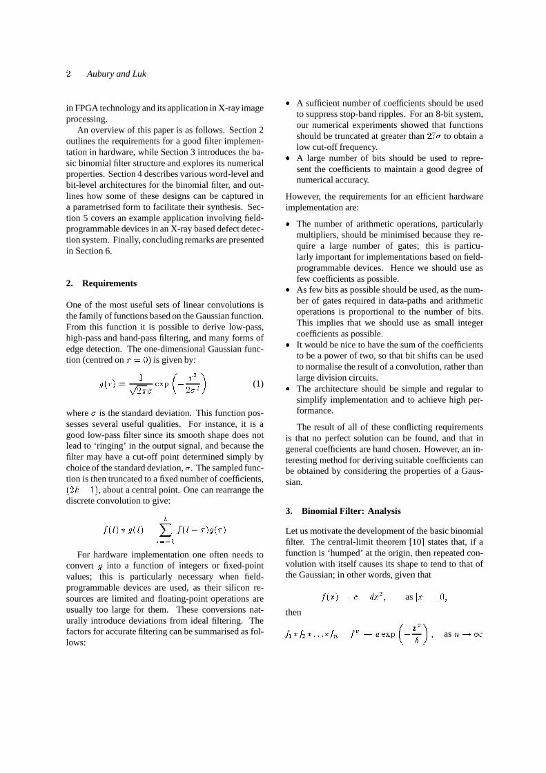
in FPGA technology and its application in X-ray imageprocessing.

An overview of this paper is as follows. Section 2outlines the requirements for a good filter implemen-tation in hardware, while Section 3 introduces the ba-sic binomial filter structure and explores its numericalproperties. Section 4 describes various word-level andbit-level architectures for the binomial filter, and out-lines how some of these designs can be captured ina parametrised form to facilitate their synthesis. Sec-tion 5 covers an example application involving field-programmable devices in an X-ray based defect detec-tion system. Finally, concluding remarks are presentedin Section 6.

2. Requirements

One of the most useful sets of linear convolutions isthe family of functions based on the Gaussian function.From this function it is possible to derive low-pass,high-pass and band-pass filtering, and many forms ofedge detection. The one-dimensional Gaussian func-tion (centred on [E\^] ) is given by:_ UV[�YK\ S` Zba;cOd�e�f g Q [�hZbc hji (1)

wherec

is the standard deviation. This function pos-sesses several useful qualities. For instance, it is agood low-pass filter since its smooth shape does notlead to ‘ringing’ in the output signal, and because thefilter may have a cut-off point determined simply bychoice of the standard deviation,

c. The sampled func-

tion is then truncated to a fixed number of coefficients,U Z�kml S*Y , about a central point. One can rearrange thediscrete convolution to give:n U!oVY;p _ U!oVY3\ qrs�t�u q

n U!o3Qwv�Y _ U�v�YFor hardware implementation one often needs to

convert _ into a function of integers or fixed-pointvalues; this is particularly necessary when field-programmable devices are used, as their silicon re-sources are limited and floating-point operations areusually too large for them. These conversions nat-urally introduce deviations from ideal filtering. Thefactors for accurate filtering can be summarised as fol-lows:

x A sufficient number of coefficients should be usedto suppress stop-band ripples. For an 8-bit system,our numerical experiments showed that functionsshould be truncated at greater than

Z!y zcto obtain a

low cut-off frequency.x A large number of bits should be used to repre-sent the coefficients to maintain a good degree ofnumerical accuracy.

However, the requirements for an efficient hardwareimplementation are:x The number of arithmetic operations, particularly

multipliers, should be minimised because they re-quire a large number of gates; this is particu-larly important for implementations based on field-programmable devices. Hence we should use asfew coefficients as possible.x As few bits as possible should be used, as the num-ber of gates required in data-paths and arithmeticoperations is proportional to the number of bits.This implies that we should use as small integercoefficients as possible.x It would be nice to have the sum of the coefficientsto be a power of two, so that bit shifts can be usedto normalise the result of a convolution, rather thanlarge division circuits.x The architecture should be simple and regular tosimplify implementation and to achieve high per-formance.

The result of all of these conflicting requirementsis that no perfect solution can be found, and that ingeneral coefficients are hand chosen. However, an in-teresting method for deriving suitable coefficients canbe obtained by considering the properties of a Gaus-sian.

3. Binomial Filter: Analysis

Let us motivate the development of the basic binomialfilter. The central-limit theorem [10] states that, if afunction is ‘humped’ at the origin, then repeated con-volution with itself causes its shape to tend to that ofthe Gaussian; in other words, given thatn U!{�Y}|�~RQ^��{ hb� as ��{���|�] �thenn�� p n h pK���*��p n N \ n N |�� d�e�f g Q {�h� i � as MP|��

Binomial Filters 3

Reversing this principle, reasonable approxima-tions to the Gaussian can be obtained by convolving asimple function with itself the desired number of times.If we take a discrete pulse (1,1) which satisfies the re-quirements of the central-limit theorem and convolveit with itself, we obtain a sequence of coefficient sets:n��

= 1n �= 1 1n h = 1 2 1n��= 1 3 3 1n��= 1 4 6 4 1n��= 1 5 10 10 5 1n��= 1 6 15 20 15 6 1

...

It is clear that the table above is Pascal’s triangle,a tabulation of the binomial coefficients. These forman increasingly good approximation to the Gaussian asmore terms are added. Since they are integers, thereis no need to worry about rounding errors, and thesum of the coefficients in each set is a power of two(it doubles at each iteration, starting from one). Thebasic binomial filter structure can be derived from thepolynomial U�S l�� u � Y Nwhich produces the binomial coefficients. This for-mula can also be regarded as a description of a cascadeof hardware units, each containing an adder and a latch– the latter for implementing the

�ju �term. Figure 1

shows an example of a binomial filter for M =4, withcoefficients (1,4,6,4,1). In this diagram, as in all othersin this paper, latches are shown as triangles with linesthrough them. Note that this structure is very sim-ple and regular; if it provides a close approximationof the Gaussian, then it would satisfy admirably ourrequirements outlined earlier.

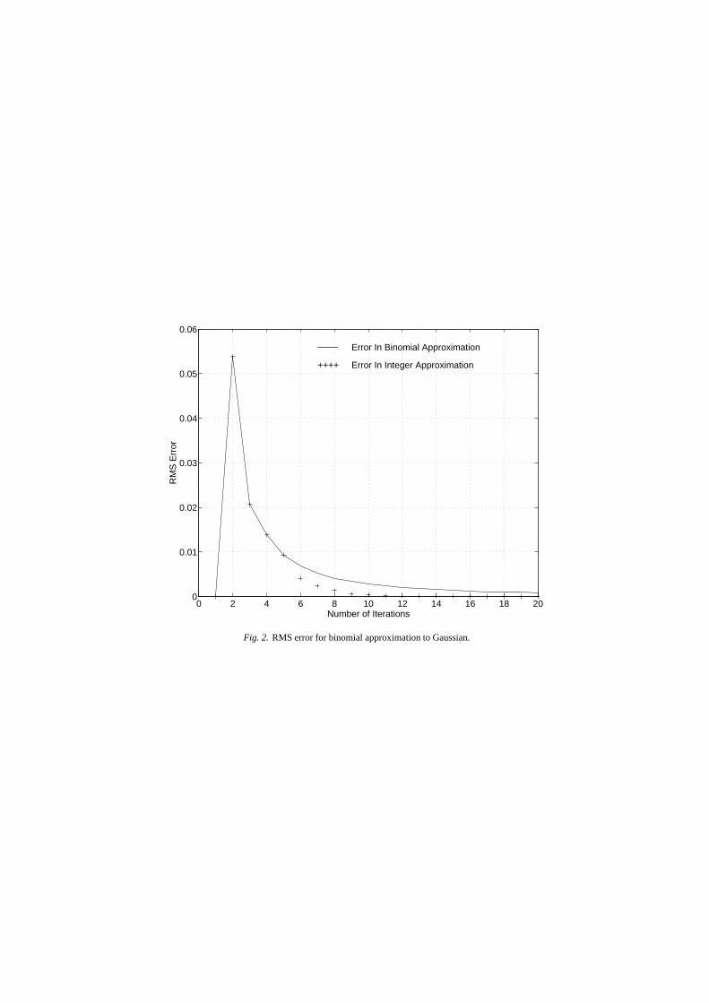
The quality of the approximation is shown in Fig-ure 2, a plot of the RMS error for each set of coefficientscompared against a Gaussian of the same variance; itis clear that the error is reduced to a very small valuefor large filters. The first zero of such a filter lies at themaximum signal frequency, and as a result there areno pass-band ripples present in the Fourier transform.The absence of truncation effects is shown in Figure 3,which shows the frequency response of

n5�ton � �

. Wecan also derive first and second differential coefficients

from the same source, by simply taking the discretedifferential of the coefficients already calculated:� U n;� Y = -1 1� U n � Y = -1 0 1� U n h�Y = -1 -1 1 1� U n5� Y = -1 -2 0 2 1� U n � Y = -1 -3 -2 2 3 1� U n;� Y = -1 -4 -5 0 5 4 1

...

or the second differentials for use in the Laplacian:� h'U n;� Y = 1 -2 1� h'U n � Y = 1 -1 -1 1� h'U n h.Y = 1 0 -2 0 1� h'U n5� Y = 1 1 -2 -2 1 1� h'U n � Y = 1 2 -1 -4 -1 2 1...

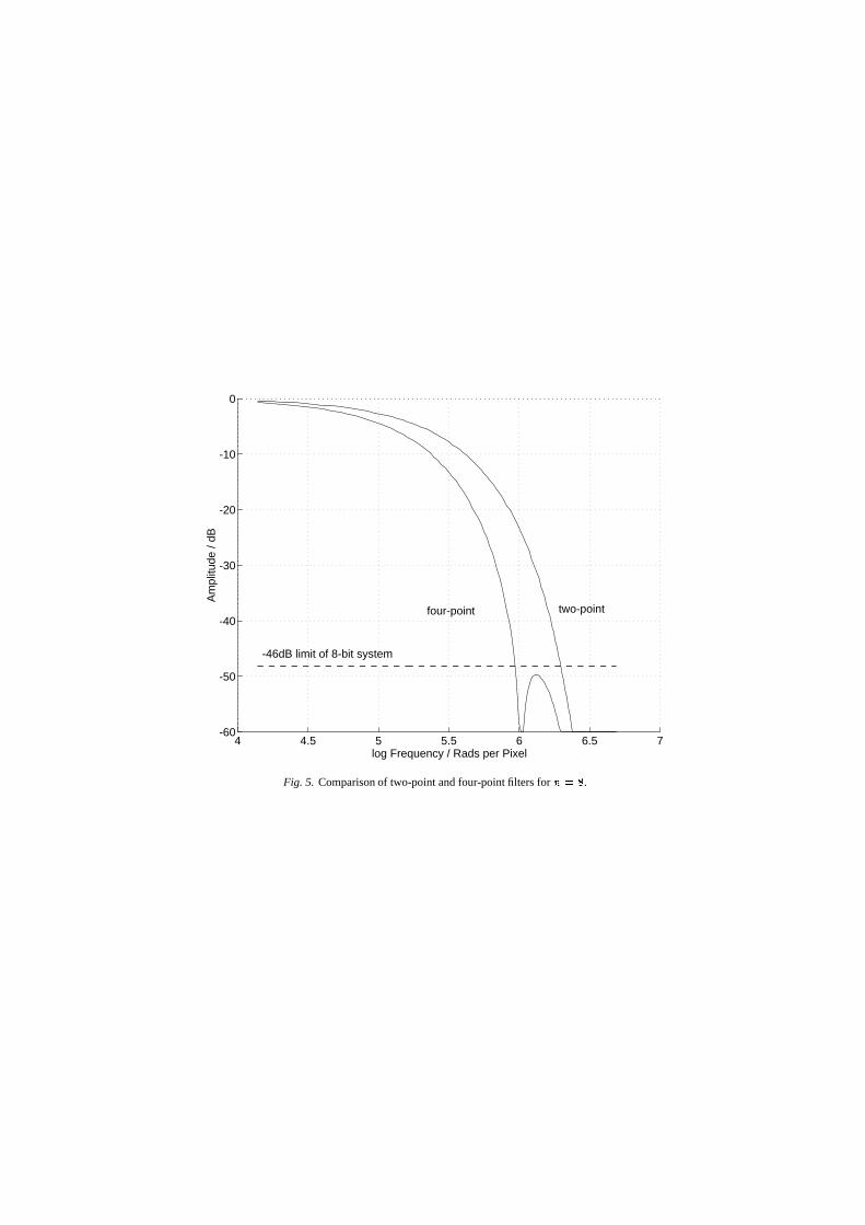
Similarly it is possible to form an approximationstarting from a four-point set of coefficients UVS � S � S � S�Y .This too satisfies the central-limit theorem, but has twozeroes in the frequency range of the system which leadsto ripples in the stop-band. However, as can be seenfrom Figure 4, repeated convolution with UVS � S�Y formore than eight times suppresses the stop-band ripplesto below the Q��j���'� dynamic range of an 8-bit sys-tem. The advantage of such four-point filters can beseen in Figure 5, which shows the frequency responseof two-point and four-point filters for MP\�� . The cut-off frequency for the four-point filter is considerablylower, without any ripples penetrating the 8-bit dy-namic range in the stop-band. Such four-point filtersare also normalisable by a power of two, and hence donot lose the benefits of the two-point filters. If verylarge filter sizes are required, it would become practi-cal to use 8-point filters possessing a low cut-off point.These filters would have to be convolved with (1,1)many times to suppress the stop-band ripples.

4. Architectures for Binomial Filters

The efficiency for a given hardware architecture de-pends on many factors, including:x Size — the number of gates and latches required to

implement a given filter.x Speed — the maximum clock rate for a given cir-cuit, normally as a function of latency and its criticalpath.

� Aubury and Luk

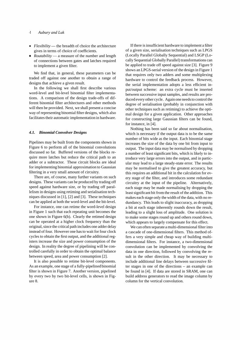
x Flexibility — the breadth of choice the architecturegives in terms of choice of coefficients.x Routability — a measure of the number and lengthof connections between gates and latches requiredto implement a given filter.

We find that, in general, these parameters can betraded off against one another to obtain a range ofdesigns that achieve a given result.

In the following we shall first describe variousword-level and bit-level binomial filter implementa-tions. A comparison of the design trade-offs of dif-ferent binomial filter architectures and other methodswill then be provided. Next, we shall present a conciseway of representing binomial filter designs, which alsofacilitates their automatic implementation in hardware.

4.1. Binomial Convolver Designs

Pipelines may be built from the components shown inFigure 6 to perform all of the binomial convolutionsdiscussed so far. Buffered versions of the blocks re-quire more latches but reduce the critical path to anadder or a subtractor. These circuit blocks are idealfor implementing binomial approximation to Gaussianfiltering in a very small amount of circuitry.

There are, of course, many further variants on suchdesigns. These variants can be produced by trading offspeed against hardware size, or by trading off paral-lelism in designs using retiming and serialisation tech-niques discussed in [1], [2] and [3]. These techniquescan be applied at both the word-level and the bit-level.

For instance, one can retime the word-level designin Figure 1 such that each repeating unit becomes theone shown in Figure 6(b). Clearly the retimed designcan be operated at a higher clock frequency than theoriginal, since the critical path includes one adder delayinstead of four. However one has to wait for four clockcycles to obtain the first output, and the additional reg-isters increase the size and power consumption of thedesign. In reality the degree of pipelining will be con-trolled carefully in order to obtain the optimal balancebetween speed, area and power consumption [2].

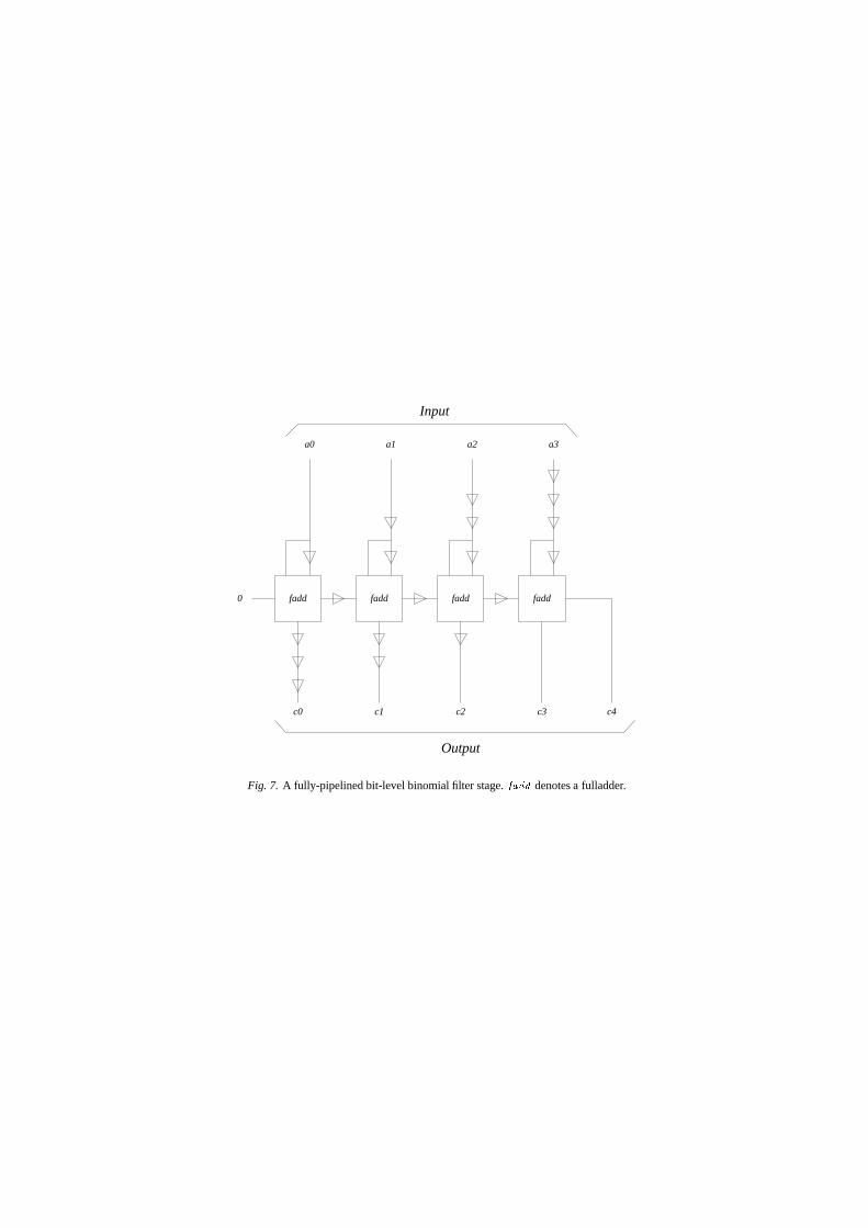
It is also possible to retime bit-level components.As an example, one stage of a fully-pipelined binomialfilter is shown in Figure 7. Another version, pipelinedby every two by two bit-level cells, is shown in Fig-ure 8.

If there is insufficient hardware to implement a filterof a given size, serialisation techniques such as LPGS(Locally Parallel Globally Sequential) and LSGP (Lo-cally Sequential Globally Parallel) transformations canbe applied to trade off speed against size [3]. Figure 9shows an LPGS-serial version of the design in Figure 1that requires only two adders and some multiplexinghardware to control the feedback process. However,the serial implementation adopts a less efficient in-put/output scheme: an extra cycle must be insertedbetween successive input samples, and results are pro-duced every other cycle. Again one needs to control thedegree of serialisation (probably in conjunction withother techniques such as retiming) to achieve the opti-mal design for a given application. Other approachesfor constructing large Gaussian filters can be found,for instance, in [4].

Nothing has been said so far about normalisation,which is necessary if the output data is to be the samenumber of bits wide as the input. Each binomial stageincreases the size of the data by one bit from input tooutput. The input data may be normalised by droppinga number of least significant bits, which is likely to in-troduce very large errors into the output, and in partic-ular may lead to a large steady-state error. The resultsmay be normalised to give the greatest accuracy, butthis requires an additional bit in the calculation for ev-ery stage of the filter, and introduces some redundantcircuitry at the input of the pipeline. Alternatively,each stage may be made normalising by dropping theleast significant bit from the result of the addition. Thismakes each stage only the width of the data, with no re-dundancy. This leads to slight inaccuracy, as droppinga bit at each stage inherently rounds down the result,leading to a slight loss of amplitude. One solution isto make some stages round up and others round down,which appears to largely compensate for this effect.

We can often separate a multi-dimensional filter intoa cascade of one-dimensional filters. This method of-fers a very simple and cheap way of building multi-dimensional filters. For instance, a two-dimensionalconvolution can be implemented by convolving thedata in one direction, followed by convolving the re-sult in the other direction. It may be necessary toinclude additional line delays between successive fil-ter stages in one of the directions – an example canbe found in [4]. If data are stored in SRAM, one canbuild address generators to read the image column bycolumn for the vertical convolution.

Binomial Filters 5

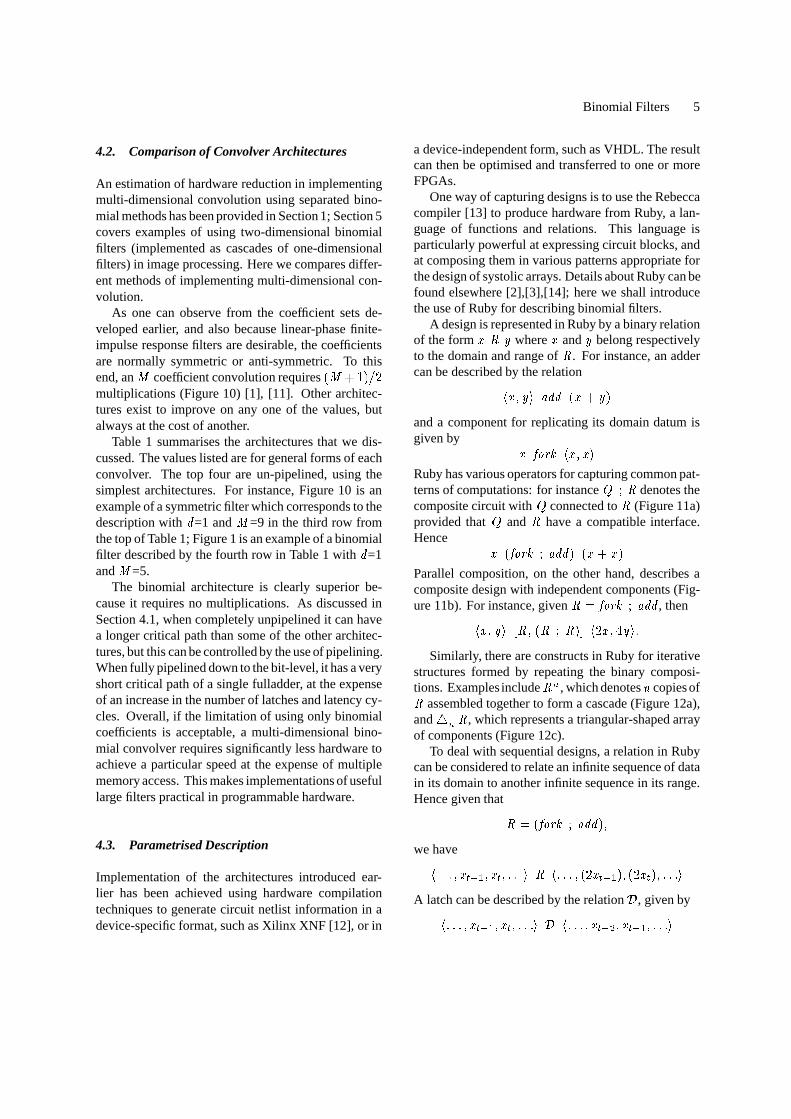
4.2. Comparison of Convolver Architectures

An estimation of hardware reduction in implementingmulti-dimensional convolution using separated bino-mial methods has been provided in Section 1; Section 5covers examples of using two-dimensional binomialfilters (implemented as cascades of one-dimensionalfilters) in image processing. Here we compares differ-ent methods of implementing multi-dimensional con-volution.

As one can observe from the coefficient sets de-veloped earlier, and also because linear-phase finite-impulse response filters are desirable, the coefficientsare normally symmetric or anti-symmetric. To thisend, an � coefficient convolution requires U�� l S�Y�� Zmultiplications (Figure 10) [1], [11]. Other architec-tures exist to improve on any one of the values, butalways at the cost of another.

Table 1 summarises the architectures that we dis-cussed. The values listed are for general forms of eachconvolver. The top four are un-pipelined, using thesimplest architectures. For instance, Figure 10 is anexample of a symmetric filter which corresponds to thedescription with � =1 and � =9 in the third row fromthe top of Table 1; Figure 1 is an example of a binomialfilter described by the fourth row in Table 1 with � =1and � =5.

The binomial architecture is clearly superior be-cause it requires no multiplications. As discussed inSection 4.1, when completely unpipelined it can havea longer critical path than some of the other architec-tures, but this can be controlled by the use of pipelining.When fully pipelined down to the bit-level, it has a veryshort critical path of a single fulladder, at the expenseof an increase in the number of latches and latency cy-cles. Overall, if the limitation of using only binomialcoefficients is acceptable, a multi-dimensional bino-mial convolver requires significantly less hardware toachieve a particular speed at the expense of multiplememory access. This makes implementations of usefullarge filters practical in programmable hardware.

4.3. Parametrised Description

Implementation of the architectures introduced ear-lier has been achieved using hardware compilationtechniques to generate circuit netlist information in adevice-specific format, such as Xilinx XNF [12], or in

a device-independent form, such as VHDL. The resultcan then be optimised and transferred to one or moreFPGAs.

One way of capturing designs is to use the Rebeccacompiler [13] to produce hardware from Ruby, a lan-guage of functions and relations. This language isparticularly powerful at expressing circuit blocks, andat composing them in various patterns appropriate forthe design of systolic arrays. Details about Ruby can befound elsewhere [2],[3],[14]; here we shall introducethe use of Ruby for describing binomial filters.

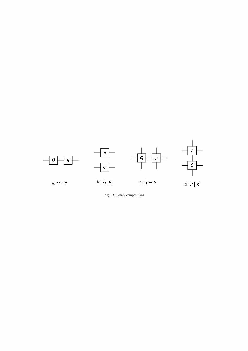
A design is represented in Ruby by a binary relationof the form { �¢¡ where { and ¡ belong respectivelyto the domain and range of � . For instance, an addercan be described by the relation£ { � ¡D¤¥���¦U!{ l ¡DYand a component for replicating its domain datum isgiven by { n*§ [ k £ { � {�¤Ruby has various operators for capturing common pat-terns of computations: for instance ¨ª©�� denotes thecomposite circuit with ¨ connected to � (Figure 11a)provided that ¨ and � have a compatible interface.Hence {«U n*§ [ k ©¬��b�jY¥U�{ l {�YParallel composition, on the other hand, describes acomposite design with independent components (Fig-ure 11b). For instance, given �­\ n�§ [ k ©��b�� , then£ { � ¡D¤¥®¯� � U!�°©G�±Y�² £ Z { � ��¡j¤ y

Similarly, there are constructs in Ruby for iterativestructures formed by repeating the binary composi-tions. Examples include �IN , which denotes M copies of� assembled together to form a cascade (Figure 12a),and ³ N � , which represents a triangular-shaped arrayof components (Figure 12c).

To deal with sequential designs, a relation in Rubycan be considered to relate an infinite sequence of datain its domain to another infinite sequence in its range.Hence given that �´\�U n*§ [ k ©¬�b��jY �we have£ ����� � {�µ u � � {*µ � ����� ¤T� £ �*��� � U Z {�µ u � Y � U Z {�µ�Y � ���*� ¤A latch can be described by the relation ¶ , given by£ �*��� � { µ u � � { µ � �*��� ¤·¶ £ �*��� � { µ u h � { µ u � � �*��� ¤

� Aubury and Luk

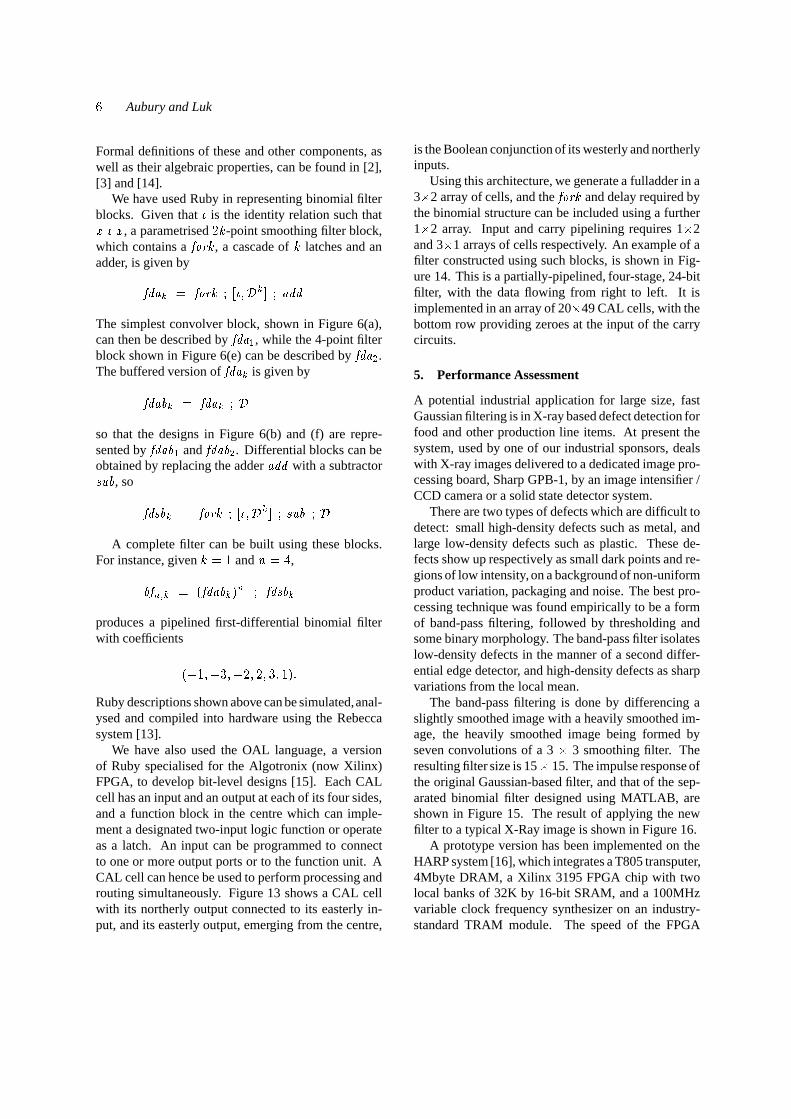
Formal definitions of these and other components, aswell as their algebraic properties, can be found in [2],[3] and [14].

We have used Ruby in representing binomial filterblocks. Given that ¸ is the identity relation such that{P¸}{ , a parametrised

Zjk-point smoothing filter block,

which contains an*§ [ k , a cascade of

klatches and an

adder, is given byn �� q \ n*§ [ k ©K®#¸ � ¶ q ²E©��b��The simplest convolver block, shown in Figure 6(a),can then be described by

n �� � , while the 4-point filterblock shown in Figure 6(e) can be described by

n �� h .The buffered version of

n �b� q is given byn �� � q \ n �� q ©5¶so that the designs in Figure 6(b) and (f) are repre-sented by

n �b� ��� andn �b� � h . Differential blocks can be

obtained by replacing the adder ��b� with a subtractor¹.º � , so n � ¹ � q \ n*§ [ k ©K®#¸ � ¶ q ²E© ¹.º � ©5¶A complete filter can be built using these blocks.

For instance, givenk \«S and MP\�� ,�%n Nb» q \¼U n �� � q Y N © n � ¹ � q

produces a pipelined first-differential binomial filterwith coefficientsU�Q½S � Qm¾ � Q Z � Z � ¾ � S.Y yRuby descriptions shown above can be simulated,anal-ysed and compiled into hardware using the Rebeccasystem [13].

We have also used the OAL language, a versionof Ruby specialised for the Algotronix (now Xilinx)FPGA, to develop bit-level designs [15]. Each CALcell has an input and an output at each of its four sides,and a function block in the centre which can imple-ment a designated two-input logic function or operateas a latch. An input can be programmed to connectto one or more output ports or to the function unit. ACAL cell can hence be used to perform processing androuting simultaneously. Figure 13 shows a CAL cellwith its northerly output connected to its easterly in-put, and its easterly output, emerging from the centre,

is the Boolean conjunction of its westerly and northerlyinputs.

Using this architecture, we generate a fulladder in a3 ¿ 2 array of cells, and the

n*§ [ k and delay required bythe binomial structure can be included using a further1 ¿ 2 array. Input and carry pipelining requires 1 ¿ 2and 3 ¿ 1 arrays of cells respectively. An example of afilter constructed using such blocks, is shown in Fig-ure 14. This is a partially-pipelined, four-stage, 24-bitfilter, with the data flowing from right to left. It isimplemented in an array of 20 ¿ 49 CAL cells, with thebottom row providing zeroes at the input of the carrycircuits.

5. Performance Assessment

A potential industrial application for large size, fastGaussian filtering is in X-ray based defect detection forfood and other production line items. At present thesystem, used by one of our industrial sponsors, dealswith X-ray images delivered to a dedicated image pro-cessing board, Sharp GPB-1, by an image intensifier /CCD camera or a solid state detector system.

There are two types of defects which are difficult todetect: small high-density defects such as metal, andlarge low-density defects such as plastic. These de-fects show up respectively as small dark points and re-gions of low intensity, on a background of non-uniformproduct variation, packaging and noise. The best pro-cessing technique was found empirically to be a formof band-pass filtering, followed by thresholding andsome binary morphology. The band-pass filter isolateslow-density defects in the manner of a second differ-ential edge detector, and high-density defects as sharpvariations from the local mean.

The band-pass filtering is done by differencing aslightly smoothed image with a heavily smoothed im-age, the heavily smoothed image being formed byseven convolutions of a 3 ¿ 3 smoothing filter. Theresulting filter size is 15 ¿ 15. The impulse response ofthe original Gaussian-based filter, and that of the sep-arated binomial filter designed using MATLAB, areshown in Figure 15. The result of applying the newfilter to a typical X-Ray image is shown in Figure 16.

A prototype version has been implemented on theHARP system [16], which integrates a T805 transputer,4Mbyte DRAM, a Xilinx 3195 FPGA chip with twolocal banks of 32K by 16-bit SRAM, and a 100MHzvariable clock frequency synthesizer on an industry-standard TRAM module. The speed of the FPGA

Binomial Filters 7

depends on the critical path of the logic that it im-plements, and it can be varied using the frequencysynthesizer. Our current experimental setup deals withreal-time video rather than X-ray images: the HARPboard takes its input from a CCD camera and sendsits result to a video display. Using this system, wehave been able to demonstrate that our binomial filterimplementation is capable of running at video rate.

Several binomial filters have also been implementedusing the CHS2 ¿ 4 FPGA-basedsystem [17]. This sys-tem contains eight CAL1024 FPGA chips arranged ina two by four array, giving 8192 user-programmablecells. A S*¾·¿ÀS*¾ pixel Gaussian smoothing filter hasbeen implemented in a PC containing a CHS2 ¿ 4 sys-tem as unseparated software, separated software, bi-nomial software and binomial hardware to compareperformance and check the results of the different im-plementations. The software is written in Microsoft Cand timed on an Intel 486DX33 based computer.

The speed of the different implementations is shownin Figure 17,excluding the downloading and uploadingtimes for the hardware implementation. It is notablethat the S�¾ ¿´S*¾ filter used by no means representsthe limit of the CHS board; it is perfectly capable ofimplementing filters upto Á]¿TÁ] pixels. This designis partially pipelined, having a critical path of around200 nanoseconds, giving a maximum running speed of5 MHz. This is far above the actual clocking speedof approximately 180 KHz, which is due to the waythe board is clocked in software by the host PC. Anexternal clocking scheme would thus allow a speed-upfactor of around thirty over the timings shown.

The filter given can also be quite easily fullypipelined, giving a maximum speed of 30 to 50(+)MHz, though at the cost of increasing latency. Thiswould give a factor of around 150 increase in speedover the times shown. The graph of Figure 18 showsthese projected speed increases against the Sharp VLSIimage processing system. If in future a CAL FPGA iscapable of accommodating an 128 ¿ 128 array of logicblocks, one can then implement on a single chip afully pipelined, 42-bit

Z �·¿ Z � filter at a pixel rate ofthe order of 30 to 100 Mpixels/s, with enhanced ac-curacy by adopting fixed-point number representation.This is one to two orders of magnitude improvementon the performance of current VLSI image process-ing systems such as the Sharp GPB-1, and it comeswith a reduction in size and an increase in flexibility.For instance, for the X-ray application it may be pos-

sible to dynamically reconfigure the FPGAs to carryout band-pass filtering, thresholding and morphologi-cal operations on the same hardware.

6. Concluding Remarks

To summarise, there are two main achievements of thiswork. First, we review a binomial approximation tothe Gaussian, and show how this architecture offersa simple, accurate and readily extensible solution sat-isfying the requirements described in Section 2. Theuse of binomial filters provides a convolution methodwhich has been shown to require considerably fewerarithmetic operations, by virtue of not requiring mul-tiplications. The resulting architecture is compact andefficient, and is readily parametrisable for a range oftrade-offs in time, space and numerical accuracy.

Second, these filters have been implemented bothin software and in several FPGA-based platforms. Forinstance, several Ruby descriptions have been imple-mented in Algotronix CAL FPGAs, and the resultsof the implementations have been verified against thesame algorithm in software. Timing of the hard-ware shows that, even when being clocked at around180kHz, a speed far below its maximum capability,it still out-performs software running on a reasonablypowerful desktop computer. Our experiments confirmthat the increase in speed achieved by using separatedfilters, binomial coefficients and the efficient binomialarchitecture can be several orders of magnitude overconventional techniques, combined with a dramatic re-duction in hardware size.

There are several areas for further research, someof which are in progress. One of our current pro-grammable hardware platforms, the CHS2 ¿ 4 [17], op-erates in a stand-alone format, with long delays in thedownloading of images for processing and in retriev-ing the results. These delays often offset the advantagegained from the efficient filtering technique. In orderfor the filters to be of practical use, the programmablehardware should be integrated into the system where itis to be used, for example as a programmable coproces-sor for existing image processing hardware. Althoughthis has been achieved to some extent in our HARP sys-tem [16] for video-rate image processing, further workis required to provide a solution for systems involvingstored data.

At present generating these filters for the targetsshown in this paper requires an in-depth understand-ing of a wide variety of tools. We are exploring the

� Aubury and Luk

development of design aids which, given a user spec-ification of a filter, will automate the parametrisation,code generation and hardware compilation steps. It isalso desirable for such tools to support data partitioning[18], hardware/software codesign [19] and, where ap-propriate, exploitation of dynamic reconfiguration ofreprogrammable FPGAs. This would make the designsystem very flexible and appealing to non-specialistsand experts alike, particularly if an integrated system,as described in the preceding paragraph, is available.

The main application for the filters described herehas been presented as image processing, but they arelikely to have considerable uses elsewhere. High speedlinear noise removal for real-time sensors [11] andshort-term memory elements for temporal neural net-works [20], are two other examples of areas in whichthese filters can offer a significant advantage over con-ventional methods.

Acknowledgements

Thanks to Jim Crowley, Keith Nishihara, Dick Shoupand members of the Oxford Hardware CompilationResearch Group for discussions and suggestions, andto the two reviewers who provided useful comments.The support of Imperial College Department of Com-puting, the ESPRIT OMI/HORN (P7249) project, Ox-ford Parallel Applications Centre, Scottish Enterpriseand Xilinx Development Corporation is gratefully ac-knowledged.

References

1. S.Y. Kung, VLSI Array Processors, Prentice Hall, 1988.2. W. Luk, “Systematic pipelining of processor arrays,” in

G.M. Megson, ed., Transformational Approaches to SystolicDesign, Chapman and Hall Parallel and Distributed Comput-ing Series, 1994, pp. 77–98.

3. W. Luk, “Systematic serialisation of array-based architec-tures,” Integration, vol. 14, no. 3, 1993, pp. 333-360.

4. H.K. Nishihara, Real-Time Implementation of a Sign-Correlation Algorithm for Image-Matching, Technical ReportNo. TR-90-02, Teleos Research, 1990.

5. W.M. Wells, “Efficient synthesis of Gaussian filters by cas-caded uniform filters,” IEEE Trans. PAMI, vol. 8, no. 2, March1992, pp. 234–239.

6. J. Canny, Finding Edges and Lines in Images, M.Sc. Thesis,Massachusetts Institute of Technology, 1983.

7. D. David, T. Court, J.L. Jacquot and A. Pirson, “INP 20: animage neighborhood processor for large kernels,” Proc. IAPRWorkshop on Computer Vision: Special Hardware and Indus-trial Applications, University of Tokyo, 1988, pp. 241-244

8. A. Chehikian and J.L. Crowley, “Fast computation of optimalsemi-octave pyramids,” 7th S.C.I.A., Aalborg, August 1991.

9. H.K. Nishihara, System for Expedited Computation of Lapla-cian and Gaussian Filtersand Correlation of Their Outputs forImage Processing, United States Patent 5119444, June 1992.

10. R.N. Bracewell, The Fourier Transform and its Applications,McGraw-Hill International, 1986

11. S. Guo, W. Luk and P. Probert, “Developing parallel architec-tures for range and image sensors,” Proc. IEEE InternationalConference on Robotics and Automation, 1994, pp. 2205–2210.

12. Xilinx Inc., The Programmable Logic Data Book, 1994.13. S. Guo and W. Luk, “Compiling Ruby into FPGAs,” to appear

in W. Luk and W.R. Moore, eds., Proc. FPL95, Lecture Notesin Computer Science, Springer Verlag, 1995.

14. G. Jones and M. Sheeran, “Circuit design in Ruby,” inJ. Staunstrup, ed., Formal Methods for VLSI Design, North-Holland, 1990, pp. 13–70.

15. W. Luk and I. Page, “Parameterising designs for FPGAs,” inW.R. Moore and W. Luk, eds., FPGAs, Abingdon EE&CSBooks, 1991, pp. 284–295.

16. A. Lawrence, A. Kay, W. Luk, T. Nomura and I. Page, “Us-ing reconfigurable hardware to speed up product developmentand performance,” to appear in W. Luk and W.R. Moore, eds.,Proc. FPL95, Lecture Notes in Computer Science, SpringerVerlag, 1995.

17. Algotronix Ltd, CHS2x4 Custom Computer User Manual,1992.

18. W. Luk, T. Wu and I. Page, “Hardware-software codesign ofmultidimensional algorithms,” in D.A. Buell and K.L. Pocek,eds., Proc. IEEE Workshop on FPGAs for Custom ComputingMachines, IEEE Computer Society Press, 1994, pp. 82–90.

19. W. Luk and T. Wu, “Towards a declarative framework forhardware-software codesign,” in Proc. Third InternationalWorkshop on Hardware/Software Codesign, IEEE ComputerSociety Press, 1994, pp. 181–188.

20. M.C. Mozer, Neural Network Architectures for Temporal Se-quence Processing, Predicting the Future and Understandingthe Past, Addison Wesley, 1993.

Matthew Aubury is a fourth year undergraduate at OxfordUniversity studying Engineering and Computing Science.He is currently working within the Hardware CompilationGroup of the Computing Laboratory on the tools used insoftware to hardware translation.

Wayne Luk studied Engineering and Computing Scienceat Oxford University and has been a faculty member there.He is currently Governors’ Lecturer at the Department ofComputing, Imperial College, University of London. Hisresearch interests include theory and practice of hardwarecompilation and hardware/software codesign.

add add add add

input output

Fig. 1. Basic binomial filter structure. The triangular blocks represent latches.

0 2 4 6 8 10 12 14 16 18 200

0.01

0.02

0.03

0.04

0.05

0.06

Number of Iterations

RM

S E

rror

____ Error In Binomial Approximation

++++ Error In Integer Approximation

Fig. 2. RMS error for binomial approximation to Gaussian.

4 4.5 5 5.5 6 6.5 7-60

-50

-40

-30

-20

-10

0

10

log Frequency / Rads per Pixel

Am

plitu

de /

dB

n=10

n=0

n=1

Fig. 3. Frequency response of+Ã&'Ä�&.0 N filter for ÅRÆTÇEÆ & Å . The dotted line indicates the -46dB dynamic range of an 8-bit system.

4 4.5 5 5.5 6 6.5 7-60

-50

-40

-30

-20

-10

0

log Frequency / Rads per Pixel

Am

plitu

de /

dB

n=0n=1

n=2

Fig. 4. Frequency response of+%&�Ä�&�Ä�&�Ä6&.06+%&�Ä%&.0 N filter for Å¬Æ Ç½Æ & Å .

4 4.5 5 5.5 6 6.5 7-60

-50

-40

-30

-20

-10

0

log Frequency / Rads per Pixel

Am

plitu

de /

dB

four-point two-point

-46dB limit of 8-bit system

Fig. 5. Comparison of two-point and four-point filters for ÇIÈ ) .

SchematicHardwarerequired Description

(a)

add

S adderS latch2-point smoothing

(b)

add

S adderZ1atches

2-point bufferedsmoothing

(c)

sub

S subtractorS latch2-point differential

(d)

sub

S subtractorZlatches

2-point buffereddifferential

(e)

add

S adderZlatches

Separated 4-pointsmoothing É

(f)

add

S adder¾ latchesSeparated 4-pointbuffered smoothing

ÊGives

+Ã&'Ä�&�Ä�&�Ä�&�0coefficients when combined with a single two-point smoothing filter

Fig. 6. Circuit blocks for constructing binomial filters. As in Figure 1, the triangular blocks represent latches.

c2c1c0 c3 c4

fadd0 fadd fadd fadd

a1 a2 a3a0

Output

Input

Fig. 7. A fully-pipelined bit-level binomial filter stage. Ë�Ì�Í.Í denotes a fulladder.

bfadd bfadd bfadd bfadd

bfadd bfadd bfadd bfadd

bfadd bfadd bfadd bfadd

bfadd

carry out

suminput

carry in

fadd

carry out

carry in

suminput

bfadd bfadd bfadd bfadd

Fig. 8. A binomial filter pipelined by every 2 Î 2 ϯË�Ì.Í�Í cells, each of which denotes a fulladder and a latch (see legend on the right of thediagram), with its horizontal inputs derived from the sum output of the Ï�Ë!Ì.Í.Í cell on its left.

~�LÐ{ Z Ñ ÒÓ Ó

�b�� Ñ ÒÓ Ó

��b�ÑÑ ÑÓFig. 9. A serial binomial filter for the coefficients (1,4,6,4,1). The component Ô6ÕKÖ�× is a multiplexer that alternately connects its output to itsbottom input and to its top input at successive clock cycles.

add add add add

0

mult

add

mult

add

mult

add

mult

add

mult

add

input

output

Fig. 10. Linear-phase filter (multiplication coefficients are not shown) – not a binomial filter.

¨ �a. ¨Ø©��

¨�

b. ®A¨ � �R²¨ �c. ¨ÚÙW�

¨�

d. ¨ÚÛK�Fig. 11. Binary compositions.

Ü Ü Üa.ÜÞÝ

Ü Ü Üb. ß½àbá Ý Ü

Ü ÜÜ ÜÜÜ

c. â Ý ÜÜÜÜ

e. ã�ä�å Ý ÜÜ Ü Ü

d. æ�ä�ç Ý ÜFig. 12. Repeated compositions.

And

Fig. 13. An example CAL cell.

Output Input

Fig. 14. Binomial filter implemented in CAL cells.

-10-5

05

10

-10

-5

0

5

100

0.005

0.01

0.015

0.02

0.025

0.03

xy

g(x,

y)

-10-5

05

10

-10

-5

0

5

100

0.005

0.01

0.015

0.02

0.025

0.03

0.035

xy

g(x,

y)

-10-5

05

10

-10

-5

0

5

10-5

-4

-3

-2

-1

0

1

x 10-3

xy

diffe

renc

e in

g(x

,y)

Fig. 15. Left: original filter impulse response; right: response of separated binomial filter; Below: error between filters

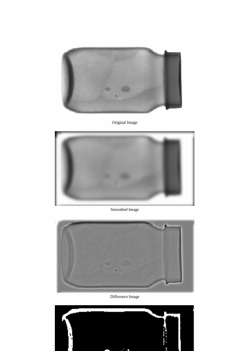
Original Image

Smoothed Image

Difference Image

Thresholded Difference Image

Fig. 16. X-ray image processed using binomial filters.

104

105

10-1

100

101

102

Number of Pixels

Tim

e T

aken

/ se

cond

s è Unseparated software filterÎ Separated software filter+ Binomial software filteré Binomial hardware filter

Fig. 17. Performance comparison of various hardware and software filters.

104

105

10-4

10-3

10-2

10-1

100

Number of Pixels

Tim

e T

aken

/ se

cond

s è Binomial filter clocked by PCÎ Binomial filter withexternal clock (projected)

+ Fully pipelined binomial filterwith external clock (projected)é Commercial VLSIimage processing system

Fig. 18. Performance comparison of various filter implementations.

Memory ê -bit ê -bit CriticalArchitecture accesses multipliers adders Latches Latency path

Unseparated S �«ë �«ë:Q´S — — —

General separated � � ��Q´S �ìê ��QíSZ v'îKï*ð µ l U!��Q´S*Y!v�ñ ë.ëSymmetric separated � � l SZ � U���Q´S*Y�ê ��QíSZ v îKï�ð µ l U�� l S�Y�v ñ ë.ë � ZBinomial separated � ] ��Q´S U���Q´S*Y�ê ��QíSZ U!��Q´S*Y!v ñ ë.ë

Word-levelpipelined binomial

� ] ��Q´S Z U��òQ­S*Y�ê ¾�U���Q´S*YZ v�ñ ë�ëFully pipelined

binomial� ] ��Q´S ó Z � ê l êìh ¾j� lÀZ êôQ zZ v6õ ñ ë�ë

Notes:öô÷is the number of coefficients used in the convolution.öôøis the number of bits used to compute the convolution, and is assumed constant (that is, each computational element normalises its

output).ö Í is the number of dimensions of convolution.öúù ñ ë.ë , ù î}ï*ð µ and

ù õ ñ ë.ë are respectively the combinational delay of an adder, a multiplier and a fulladder. Wire delays are ignored in theestimation of critical path.öLatency is defined to be the number of cycles between a number being input and its reaching the centre of a set of coefficients.öFor the unseparated filter, the number of latches and the latency is dependent upon the dimensions of the input data.öThe exact number of latches for a fully pipelined binomial architecture is

ø:ûÞü × ÷ øþý ÷ ý ÿ�ø ü &.

Table 1. Comparison of architectures.