Bilinear modelling of batch processes. Part I: theoretical discussion

299

Research Article

Received: 28 November 2006; Revised: 7 September 2007; Accepted: 29 November 2007 Published online in Wiley Interscience: 2008

(www.interscience.wiley.com) DOI: 10.1002/cem.1113

Bilinear modelling of batch processes. Part I:theoretical discussionJose Camachoa∗, Jesus Picoa and Alberto Ferrerb

When studying the principal component analysis (PCA) or partial least squares (PLS) modelling of batch processdata, one realizes that there is a wide range of approaches. In many cases, new modelling approaches are presentedjust because they work properly for a particular application, for example, on-line monitoring and a given numberof processes. A clear understanding of why these approaches perform successfully and which are the advantagesand disadvantages in front of the others is seldom supplied. Why does modelling after batch-wise unfolding capturechanging dynamics? What are the consequences of variable-wise unfolding? Is there any best unfolding method?When should several models for a single process be used? In this paper, it is shown how these and other relatedquestions can be answered by properly analyzing the dynamic covariance structures of the various approaches.Copyright © 2008 John Wiley & Sons, Ltd.

Keywords: principal component analysis; partial least squares; batch processes; unfolding methods

1. INTRODUCTION

Industrial batch processes produce a enormous amount of three-way data which is recorded for on-line treatment or posterioranalysis. These are, nonetheless, difficult tasks due to the volumeof the data and a low signal-to-noise ratio. One of the mostwidely used methods to extract the information from that kindof data are the projection to latent structures-based methods(PLS-based), like principal component analysis (PCA) and partialleast squares (PLS). Since the duration of the processing of a batchmay be variable in some processes, data have to be properlyaligned—equalized—to apply most PLS-based methods. Severalaligned methods can be found in the literature [1–6]. Afterthe alignment, the data matrix of a batch process X (I × J × K )contains the values of J variables at K sampling times in I batches.

Optionally, a number of initial conditions and qualitymeasurements may be collected in a process. The L initialconditions measured for the I batches are arranged in matrix Z(I ×L). The M quality variables, collected at Ky sampling times, arestored in matrix Y (I × M × Ky ). Commonly, the quality variablesare only measured at the end of the batch. Therefore, they maybe arranged in a two-way matrix Y (I × M).

The approaches for modelling batch processes with PLS-basedmethods can be roughly classified into two categories: The singlemodel approach and the multi-model approach.

In the single model approach, a single PLS-based model isgenerated for the whole process. Although three-way modellingmethods exist [7–10], the most commonly used procedure is tounfold the three-way matrix of data in two dimensions [11,12].Afterwards, a bilinear model such as PCA or PLS can be fitted.

When using a single bilinear model, the direction of unfoldingdepends on the variability which is wanted to be modelled.According to Reference [13], for the treatment of batch processdata, only batch-wise unfolding (1) and variable-wise unfolding(2) have interest

X (I × J × K) ⇒ X(I × JK) (1)

X(I × J × K) ⇒ X(KI × J) (2)

where X is the unfolded two-way matrix of data. Batch-wiseunfolding treats the data of a complete batch as an object (row)of the resulting two-way matrix of data (see Figure 1(a)). Variable-wise unfolding treats data collected each sampling time of abatch as an object (Figure 1(b)). Moreover, since data are usuallycentred and scaled to unit variance after the unfolding operation,additional differences between both unfolding methods arefound because of the preprocessing.

The direction of unfolding also influences the design of anon-line application. If batch-wise unfolding is used [1], themeasurements which are not available have to be imputed atevery sampling time. The methods designed to impute missingdata from a PCA and PLS model [14,15] can be used for thispurpose. If variable-wise unfolding is used no imputation isnecessary, but the dynamics of the process in the form of auto-covariances and lagged cross-covariances among variables arenot captured [13]. Some authors have proposed to combineboth unfolding methods. In Reference [3], three monitoring levelsare generated, where only the first two are used for on-linemonitoring. The level 1 consists of a variable-wise model. Thus,it does not take into account the auto-covariances and laggedcross-covariances. The level 2 uses the scores obtained from theprevious model to generate the monitoring charts. This is carried

* Departamento de Ingenierıa de Sistemas y Automatica, Universidad Politecnicade Valencia, Valencia, Spain.E-mail: [email protected]

a J. Camacho, J. PicoDepartamento de Ingenierıa de Sistemas y Automatica, Universidad Politecnicade Valencia, Valencia, Spain

b A. FerrerDepartamento de Estadıstica e Investigacion Operativa Aplicadas y Calidad,Universidad Politecnica de Valencia, Valencia, Spain

J. Chemometrics2008; 22: 299–308 Copyright © 2008 John Wiley & Sons, Ltd.

300

J. Camacho, J. Pico and A. Ferrer

Figure 1. Different arrangements of three-way batch data in two-way form. (a) batch-wise unfolding, (b) variable-wise unfolding, (c) batch dynamicunfolding with 1 LMV, (d) K-models approaches. In (d), from left to right, the data used to fit a local model, an evolving model and a moving windowmodel for sampling time k are represented. This Figure is available in colour online at www.interscience.wiley.com/journal/cem

out by rearranging the scores as in batch-wise unfolding. Theauthors also conceive the possibility of generating a PCA modelfrom these rearranged data. By doing so, auto-covariances andlagged cross-covariances of the scores of level 1 are capturedin the level 2 [3]. Alternatively, Reference [16] proposes totake advantage of both batch-wise and variable-wise unfoldingprocedures by generating two models from the original data, oneafter each unfolding.

Batch dynamic PCA (BDPCA) and batch dynamic PLS (BDPLS)[17] are another single-model approaches equivalent to thevariable-wise unfolding with the addition of lagged measurementvectors (LMVs) as variables [18]. An example of this unfolding with1 LMV is shown in Figure 1(c). The batch dynamic unfolding can beseen as a generalization of the traditional unfolding procedures:if no LMV is added, the resulting matrix is the same as the oneafter variable-wise unfolding; if all possible LMVs are added, theresulting matrix is the same as the one after batch-wise unfolding.

The multi-model approach is traditionally based on thegeneration of a bilinear model for every sampling time of thebatch duration [19–21]. This is referred here as the K-modelsapproach (Figure 1(d)). These models do not need to imputemeasurements and are able to capture the dynamics by includingLMVs as variables, but the price to pay is the generation ofthat high number of models. Again, several proposals can befound in the literature, which mainly differ in the data usedto generate the sub-models. If each sub-model includes onlythe data of a sampling time, then it is called a local model.If each sub-model incorporates the measurements from the

beginning of the batch to a sampling time, then it is called anevolving model [20]. Hierarchical models [19] follow the lattermethod but giving different weight to the current measurementsof the variables. This is done by calculating the scores in ahierarchical fashion. Finally, if only the immediate part of the pastmeasurements is included in each sub-model together with thecurrent measurements, the procedure is called moving windowPCA (MWPCA) [21] or moving window PLS (MWPLS).

One of the most appreciated benefits of using PLS-basedtechniques is that, by conveniently studying the fitted model,the process understanding can be improved [22]. Althoughthe calibration of a sub-model for each sampling time can beadvantageous for the on-line application, such a number of sub-models can be complex to handle and difficult to interpret.Recently, the use of a reduced number of sub-models, eachone representing a certain period of the process, has beenstudied. In References [16] and [23], authors propose the useof a sub-model for every processing unit of the process. Also,several sub-models can be defined for a single processing unitif necessary. Reference [24] proposes a clustering algorithm forthe automatic identification of a number of sub-models for on-line monitoring. The same objective is pursued in Reference [18],where the sub-models are identified using the multi-phase PCAalgorithm [25].

In this paper, a theoretical discussion regarding the differencesamong the principal modelling approaches is carried out bystudying the structure of the resulting covariance matrix. Thisdiscussion is limited to bilinear and non-hierarchical PLS-based

www.interscience.wiley.com/journal/cem Copyright © 2008 John Wiley & Sons, Ltd. J. Chemometrics 2008; 22: 299–308

301

Bilinearmodellingofbatchprocesses: Part I

models. In Section 2, some useful notation is introduced. InSection 3, the use of the covariance matrix for the analysis ofbilinear methods is briefly discussed. In Section 4, the singlemodel approach is studied. In Section 5, the multi-modelapproach based in the design of a single PLS-based model forevery sampling time, that is, the K-models approach, is analysed.In Section 6, the multi-phase modelling approach is presented.Finally, Section 7 gives some conclusions.

2. SOME NOTATION

To apply a bilinear modelling method, data in matrix X (I × J × K )have to be rearranged in two dimensions. This can be achievedby unfolding X , by dividing X in a number of two-way matrices orby a combination of both.

2.1. Unfolding

The batch dynamic unfolding can be expressed as

X = unfold (X, n) ≡ X (n) (3)

where n stands for the number of LMVs included as variables and

n = {k − 1 : k � {1, 2, . . . , K}} (4)

Therefore, the batch-wise unfolding is

X = X (K−1) (5)

and the variable-wise unfolding

X = X (0) (6)

2.2. Number of sub-matrices

Let X ki :kecontain the data of X from sampling time ki to ke . One

way to arrange X in two-way is to divide the data in K local sub-matrices

X = {X k : k = 1, . . . , K} (7)

where X k ≡ X (0)k .

Combining the unfolding with the division in several sub-matrices, many other approaches can be specified. For instance,the Evolving approach

X = {X (k−1)

1:k : k = 1, . . . , K}

(8)

3. STUDY OF THE COVARIANCE MATRIX

Strictly speaking, the analysis carried out in this paper is focusedon matrix X T · X . This matrix is the same, but a constant factor, tothe covariance matrix of X when it is centred. By inspecting X T ·X the dynamic and static relationships among process variablesbuilt in a model can be observed.

The analysis of X T · X is valid to understand the dynamics builtin PCA models (and so it is for principal components regression(PCR) models). In the case of PLS, let us assume the matrix X T · Y ·Y T · X is used to fit the models. Making the change of variable C =Y T · X it can be seen that PLS is performed over CT · C. Therefore,the conclusions drawn from X T · X are also valid for PLS but withthe difference that in the latter the relationships are not among

original process variables, but among covariance values betweenprocess and quality variables.

4. SINGLE MODEL APPROACH

Two traditional methods have been proposed for the end-of-batch and on-line monitoring of batch processes: the approachof Nomikos and MacGregor [1,11] and the approach of Wold et al.[3]. The principal difference between these methods is found inthe modelling for on-line monitoring. In Reference [1], the batch-wise unfolding (Figure 1(a)) procedure is used. In Reference [3],the variable-wise unfolding (Figure 1(b)) is used as first step tocreate the monitoring system. In both cases, the unfolded dataare auto-scaled, that is, each variable of the unfolded matrix iscentred and scaled to unit variance. This implies that the bilinearmodels in both approaches are modelling different data, since forthe first approach the average trajectory of the process variablesis subtracted whereas for the second one it is not. Therefore, theinfluence of the unfolding direction and of the preprocessingmethod in the differences found between both proposals is notclearly distinguishable.

Although the implications of the unfolding direction in a on-line system have been pointed out by several authors [3,13,26]and introduced in the first section of this paper, here this issue ismore deeply revisited focusing on the structure of the resultingcovariance matrices and with an independent point of view fromthe preprocessing mechanism. Furthermore, these implicationsdo not seem to be very well understood by part of the researchcommunity yet. For instance, some authors believe that bybatch-wise unfolding, the resulting model does not include thedynamics of the variation around the average trajectory [17]. Itwill be shown that this conclusion is wrong.

In the following, let imagine the matrix X corresponds to thedata collected from a batch process after the subtraction of theaverage trajectory.†

4.1. Batch-wise unfolding

In Figure 2, the resulting JK × JK covariance matrix after thebatch-wise unfolding of the data, that is, X (K−1) (Figure 1(a))is shown. It can be seen that the relationships among all thevariables at different sampling times are modelled by the PCAperformed with this matrix. These relationships include thevariances and instantaneous cross-covariances of the variablesat every sampling time—represented by the square sub-matrices {VC1 · · · VCK } in the diagonal—along with the auto-covariances and lagged cross-covariances of the variables—relationships outside these sub-matrices. Sub-matrices Vk,k+d

for k = 1, . . . , K − d contain the auto-covariances and cross-covariances of order d. In Figure 2, only sub-matrices Vk,k+1 aredrawn for the shake of simplicity.

The dynamics of the variation around the average trajectory arerepresented by the relationships in sub-matrices Vk,k+d . It can beconcluded that, unlike some authors have claimed, batch-wiseunfolded models do incorporate the linear dynamics (aroundthe average trajectory) of the process. Furthermore, these modelsare able to capture changing relationships among variables, sincesub-matrices VCk and Vk,k+d for two different values of k—say 1

† The average trajectory is subtracted so that the resulting two-way matrix afterboth batch-wise and variable-wise unfolding is centred and the same data aremodelled.

J. Chemometrics. 2008; 22: 299–308 Copyright © 2008 John Wiley & Sons, Ltd. www.interscience.wiley.com/journal/cem

302


Figure 2. Covariance matrix after the subtraction of the averagetrajectory and batch-wise unfolding. This Figure is available in colouronline at www.interscience.wiley.com/journal/cem

and 10—are placed in different parts of the covariance matrix,and so treated independently.

4.2. Variable-wise unfolding

The J × J covariance matrix obtained after variable-wiseunfolding, that is, X (0) (Figure 1(b)) is equivalent, but a constantfactor equal to 1

K, to the sum of the matrices {VC1 · · · VCK }

(see Figure 3). This has two consequences: first, variable-wisemodels only incorporate the variances and instantaneous cross-covariances of the variables and not the dynamics; and second,each relationship between a pair of variables in the covariancematrix is an average of their relationship throughout the batchduration. Thus, this modelling strategy is only valid when thecorrelation structure of a process is more or less constant. Onthe other hand, the number of batches required to generatea model in variable-wise unfolding is lower than in batch-wiseunfolding. After the former unfolding, for every batch, a numberof objects equal to the length of the batch is available. In batch-wise unfolding, a batch is a single object.

4.3. Batch dynamic unfolding

The batch dynamic unfolding is equivalent to the variable-wise unfolding with LMVs addition [18]. Figure 4 shows thecorresponding covariance matrix after data have been unfolded

Figure 3. Covariance matrix after the subtraction of the averagetrajectory and variable-wise unfolding.

following the example in Figure 1(c), X (1). From this Figure it iseasy to understand the effect of the addition of LMVs. Dynamicsof order d are built in the model by matrices Vk,k+d . The more LMVsadded, the more dynamic information included in the model. Asstated in Reference [25], depending on the nature of the process,part of the dynamic information may be negligible and it could beadvantageous not to incorporate it to the model. Thus, identifyingthe optimum number of LMVs from the data of a process is,a priori, a more powerful modelling approach than using anextreme case, like in batch-wise or variable-wise unfolding.

It should be pointed out that when the number of LMVs is low,the resulting batch dynamic model is very close to the traditionalway of modelling the dynamics with autoregressive models. Auto-correlations and cross-correlations are obtained independently ofthe precise sampling time. This model structure is very useful forregulation and can be used to relax the necessity of alignmentof the batches [5]. Nonetheless, as it happens for variable-wiseunfolded models, modelling with a reduced number of LMVsassumes a constant correlation structure during the batch. Themore LMVs included in the model, the less the number of objects-rows- in the unfolded matrix—X (n) has I(K − n) rows. Therefore,by adding LMVs, the interval where the correlation structureis imposed to be constant is reduced and the model is morecapable to capture changes in the dynamics. At the same time, thedynamics built in the model are more dependent on the precisesampling time. A batch dynamic model of the form X (n) assumesthe dynamics of the process can be considered time-invariant fora K − n sampling times period.

Although batch dynamic unfolding provides the possibilityto capture time-varying correlation structures by adding asufficient number of LMVs, this may lead to over-parameterizedmodels. Take the extreme example of a process in which time-varying but only static relationships among variables exist. Thisprocess can be modelled by batch-wise unfolding the data andapplying a bilinear PLS-based method. Then, time-varying staticrelationships will be effectively modelled by matrices VCk inFigure 2. Nonetheless, the rest of the covariance matrix will bejust noise, since there are not significant dynamic relationships.

5. K-MODELS APPROACH

The K-models approach (see Figure 1(d)) is based on generatinga single sub-model for every sampling time. Local models [20]are the simplest example of this approach, where the sub-model associated to a sampling time is computed from the datacollected at that sampling time alone. Data are split accordingto Equation (7). Nonetheless, the inclusion of the dynamics ofthe process can be crucial for a good modelling performance.A straightforward alternative to local modelling is evolvingmodelling [20], where all the possible LMVs are included in asub-model as additional variables (8).

More sophisticated approaches can be used. Not all the laggedinformation may be of interest or at least be given the sameimportance in every sub-model. Uniformly weighted moving

Figure 4. Covariance matrix after the subtraction of the average trajectory and batch dynamic unfolding according to Figure 1(c).


303


Figure 5. Addition of 1 LMV to the local matrix of data at sampling timek: as additional variables, columns (a) and as additional objects, rows (b).

window (UWMW) or Exponentially weighted evolving window(EWEW) models may be defined in order to better adjust themulti-model to the nature of the process. UWMW modelling usesthe current data along with those of the immediate nk LMVs togenerate the current sub-model

X = {X k−nk :k : k = 1, . . . , K} (9)

nk is the size of the window, a calibration parameter of the UWMWmodel.

An EWEW sub-model includes all the lagged measurements tothe current sampling time:

X = {X1:k � W1:k : k = 1, . . . , K} (10)

where W1:k is a weighting matrix and � stands for the Hadamard(element to element) product. W1:k is constructed according toan exponentially decreasing value, the forgetting factor �k � [0, 1],so that each measurement losses importance as the processadvances. The weight of the measurement-vector collected attime k − d, for the generation of the sub-model at time k, is (�k )d ,being the weight of the current measurements always (�k )0 = 1.

The parameters nk and �k in UWMW and EWEW models arecalibrated independently for every single sub-model—that is whythe subscript k is used—for instance by using cross-validation.

Additionally, there are two ways to carry out the inclusion oflagged measurements: as additional variables—columns—or asadditional objects—rows—of the unfolded matrix. In Figure 5,these two ways are shown for the addition of 1 LMV to the currentmeasurement vector at sampling time k.

In Figure 6, the covariance matrices of an UWMW model for theinclusion of the lagged measurements as variables or objects, areshown. Both arrangements can be respectively noted as

X = {X (nk )k−nk :k : k = 1, . . . , K} (11)

and

X = {X (0)k−nk :k : k = 1, . . . , K} (12)

Figure 6. Covariance matrices of UWMW models: LMVs added asvariables, columns (a) or as objects, rows (b). n is the size of thewindow. This Figure is available in colour online at www.interscience.wiley.com/journal/cem

In Figure 7, the same is shown for an EWEW model. Also, botharrangement approaches can be noted as:

X = {X (k−1)

1:k � W (k−1)1:k : k = 1, . . . , K

}(13)

and

X = {X (0)1:k � W (0)

1:k : k = 1, . . . , K} (14)

Figure 7. Covariance matrices of EWEW models: LMVs added asvariables, columns (a) or as objects, rows (b). � is the forgettingfactor. This Figure is available in colour online at www.interscience.wiley.com/journal/cem


304


The two modelling approaches have different properties. TheEWEW models take into account all the past information. Thus,they handle a bigger amount of data than UWMW models andso they are more computationally demanding. Nonetheless, arecursive PLS algorithm [27,28] may be applied to reduce thatcomplexity. Both UWMW and EWEW coincides for �k = 0 andnk = 0, values for which they become local models, and for�k = 1 and nk = k − 1, for which they become evolving modelswhen the LMVs are included as variables. Therefore, EWEW andUWMW strategies can be seen as a general parametrization whereevolving and local models are extreme cases.

Comparing the covariance matrices of Figures 6(a) and 7(a)with those of Figures 6(b) and 7(b), it should be stressedthat the inclusion of LMVs as variables is more similar to thebatch-wise unfolding, whereas the effect of this inclusion asadditional objects resembles the case of variable-wise unfolding.A direct conclusion might be extracted: the dynamic informationcontained in the auto-covariances and lagged cross-covariances isnot captured with the inclusion of lagged objects. Notice that thisinformation is contained in the sub-matrices of the general formVt,t+d , which are only present in the covariance matrices of Figures6(a) and 7(a). Since the dynamics are important in the modelling,a poor modelling performance of the approaches which do notinclude lagged variables is expected.

Finally, in Reference [19] a hierarchical K-models approach ispresented. The basis of this approach is to combine the pastand local information with an adaptive hierarchical PCA model.The model for every sampling time is obtained from the highlevel loadings of the immediate past sampling time model andthe measurements collected at the current sampling time. Theanalysis of this approach from the covariance matrix is not trivialand it is not performed here. Nonetheless, in the companionpaper, two extensions of this approach to PLS are compared withthe other models studied here and differences are highlighted.

6. MULTI-PHASE APPROACH

The multi-phase approach is proposed to overcome theshortcomings of the single model approach with a reducednumber of sub-models. First, batch-wise models may not performadequately when several periods of the batch process arenonlinearly related or independent [25]. This is discussed inSection 6.1. Second, as commented before, variable-wise modelscannot capture changing correlation structures and processdynamics. This is further studied in Section 6.2. Finally, batchdynamic models can be affected by both nonlinearity orindependence and changes in the correlation structure, as it willbe explained in Section 6.3. In the three cases, the model can beimproved by modelling independently periods of the batch: thephases.

Let us define a phase as a segment of the batch duration whichis well approximated by a single linear model. From this definitionit should be stressed that the optimum division in phases of aprocess depends on the structure of the linear models used. Usingbatch-wise models, the phases are periods where the variablesare linearly related. Using variable-wise models, the phases areperiods with a constant correlation structure. Finally, for batchdynamic models, the phases are periods with constant dynamicsand where the current and immediate preceding n LMVs arelinearly related.

The multi-phase modelling approach provides more flexiblemodels than the single model and K-models approaches.Nonetheless, we are aware that it has also its limitations. First,as it is well known, the use of local linear models for modellingnonlinearity does not take into account part of the multivariatenature of the data, that is, when approximating nonlinearitywith local models, part of the information is lost. Second, thechanges in the correlation structure of a batch may be smooth.In that case, smooth transitions between sub-models maybe more adequate than a crisp division in phases. Althoughsmooth transitions can be achieved with the currently availablemodelling techniques, for instance by using the Fuzzy theoryor the Mixtures of Probabilistic PCA [29], it should be notedthat these methodologies may complicate the use and easyinterpretation of the models. The use of fuzzy logic for multi-phase modelling was originally proposed in Reference [25] andhas been recently investigated in Reference [30].

6.1. Phases in batch-wise data

When data include independent or nonlinearly related groups ofvariables, a different model should be designed for each of thesegroups. This is discussed in detail in Reference [25]. Nonlinearrelationships and independence between two variables areexamples of relationships poorly approximated with a linearmodel. The variables so related show low correlation values.In batch processes, two observations of the vector of processvariables commonly show less correlation as the time (gradeof completion of the batch) distance between them grows. InFigure 8, the correlation map of the batch-wise unfolded data oftwo variables, collected from a polymerization process, is shown.This is a well-known real data set of 50 batches provided byDupont Co. For more details of the process or the data set, see[22]. The data is aligned to a batch length of 116 sampling times.The result of the batch-wise unfolding is a bi-dimensional matrixwith 50 observations of 232 variables, ordered as depicted inFigure 1(a).

The Figure shows a diagonal of high correlation. The darkrectangles of the graphic represent the segments of the batchwhere the variables are highly correlated with their precedingvalues. The correlation gets negligible as the time distance grows.The formation of rectangles in the correlation map means that

Figure 8. Correlation of two variables measured 116 times (batchduration) after batch-wise unfolding and preprocessing (auto-scaling).Nylon 6′6 cultivation process. This Figure is available in colour online atwww.interscience.wiley.com/journal/cem


305


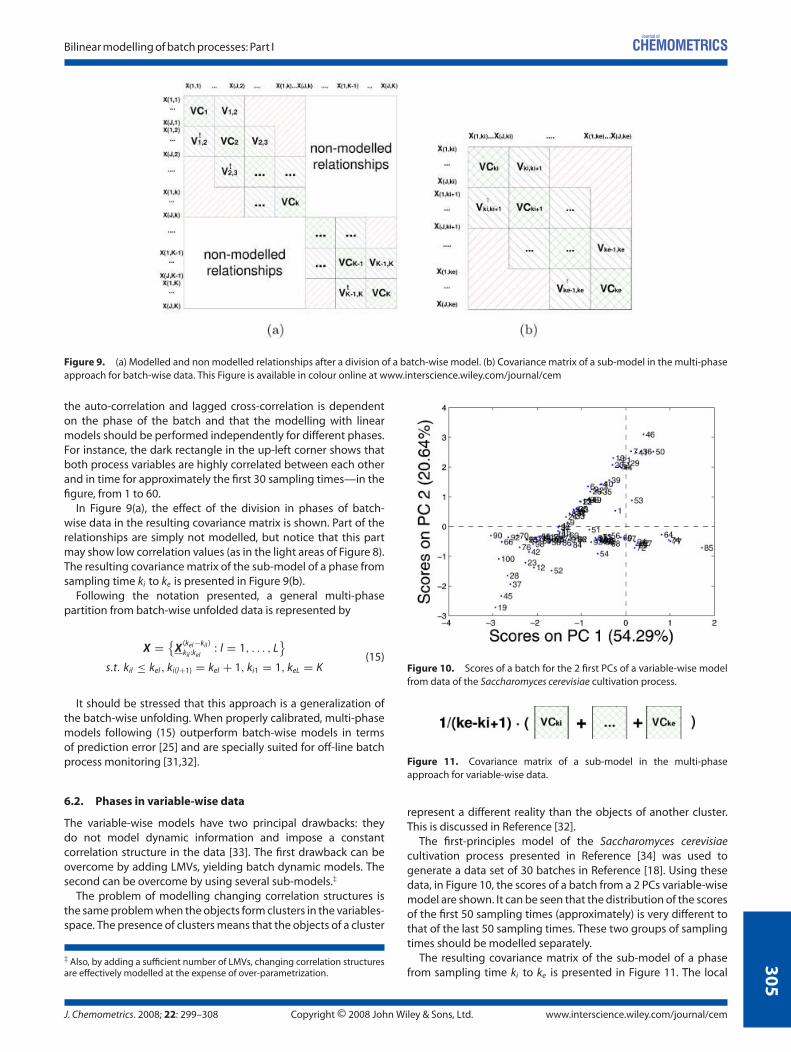
Figure 9. (a) Modelled and non modelled relationships after a division of a batch-wise model. (b) Covariance matrix of a sub-model in the multi-phaseapproach for batch-wise data. This Figure is available in colour online at www.interscience.wiley.com/journal/cem

the auto-correlation and lagged cross-correlation is dependenton the phase of the batch and that the modelling with linearmodels should be performed independently for different phases.For instance, the dark rectangle in the up-left corner shows thatboth process variables are highly correlated between each otherand in time for approximately the first 30 sampling times—in thefigure, from 1 to 60.

In Figure 9(a), the effect of the division in phases of batch-wise data in the resulting covariance matrix is shown. Part of therelationships are simply not modelled, but notice that this partmay show low correlation values (as in the light areas of Figure 8).The resulting covariance matrix of the sub-model of a phase fromsampling time ki to ke is presented in Figure 9(b).

Following the notation presented, a general multi-phasepartition from batch-wise unfolded data is represented by

X = {X

(kel−kil )kil :kel

: l = 1, . . . , L}

s.t. kil ≤ kel, ki(l+1) = kel + 1, ki1 = 1, keL = K(15)

It should be stressed that this approach is a generalization ofthe batch-wise unfolding. When properly calibrated, multi-phasemodels following (15) outperform batch-wise models in termsof prediction error [25] and are specially suited for off-line batchprocess monitoring [31,32].

6.2. Phases in variable-wise data

The variable-wise models have two principal drawbacks: theydo not model dynamic information and impose a constantcorrelation structure in the data [33]. The first drawback can beovercome by adding LMVs, yielding batch dynamic models. Thesecond can be overcome by using several sub-models.‡

The problem of modelling changing correlation structures isthe same problem when the objects form clusters in the variables-space. The presence of clusters means that the objects of a cluster

‡ Also, by adding a sufficient number of LMVs, changing correlation structuresare effectively modelled at the expense of over-parametrization.

Figure 10. Scores of a batch for the 2 first PCs of a variable-wise modelfrom data of the Saccharomyces cerevisiae cultivation process.

Figure 11. Covariance matrix of a sub-model in the multi-phaseapproach for variable-wise data.

represent a different reality than the objects of another cluster.This is discussed in Reference [32].

The first-principles model of the Saccharomyces cerevisiaecultivation process presented in Reference [34] was used togenerate a data set of 30 batches in Reference [18]. Using thesedata, in Figure 10, the scores of a batch from a 2 PCs variable-wisemodel are shown. It can be seen that the distribution of the scoresof the first 50 sampling times (approximately) is very different tothat of the last 50 sampling times. These two groups of samplingtimes should be modelled separately.

The resulting covariance matrix of the sub-model of a phasefrom sampling time ki to ke is presented in Figure 11. The local


306


Figure 12. Covariance matrix of a sub-model in the multi-phase approach for batch dynamic data.

models of the single sampling times are averaged as in variable-wise unfolding.

A general multi-phase partition from variable-wise unfoldeddata is represented by

X = {X (0)

kil :kel: l = 1, . . . , L

}

s.t. kil ≤ kel, ki(l+1) = kel + 1, ki1 = 1, keL = K(16)

6.3. Phases in batch dynamic data

The resulting covariance matrix of the sub-model of a phase fromsampling time ki to ke , for batch dynamic data, is presented inFigure 12. The covariance matrices of the UWMW models of thesingle sampling times—from ki to ke—are averaged.

The multi-phase models based on batch dynamic data useseveral sub-models for capturing changing correlation structures.The auto-covariances and lagged cross-covariances are modelledby including LMVs as variables. The size of the window n

depends on the amount of past information needed. Eachsub-model can have a different optimum n value. By properlycalibrating this parameter, problems with nonlinear relationshipsor independence are also avoided.

A general multi-phase partition from batch dynamic unfoldeddata is represented by

X = {X

(nl )max(kil−nl ,1):kel

: l = 1, . . . , L}

(17)

with

nl = {k − 1 : k � {1, 2, . . . , kel}}s.t. kil ≤ kel, ki(l+1) = kel + 1, ki1 = 1, keL = K

(18)

Notice that the sub-models are not completely disjoint, since nl

measurement vectors are used to fit both sub-models l − 1 and l.The matrix of Figure 11 is a particular case (for n = 0) of that

of Figure 12. Nonetheless, a multi-phase partition of batch-wisedata (Figure 9) cannot be seen as a particular case of the multi-phase partition of batch dynamic data. This is a consequence ofthe definition in Equations (17) and (18). In this definition, theonly possibility of obtaining disjoint sub-models is for variable-wise unfolding, that is, nl = 0 for l � {1, 2, . . . , L}. Therefore, themulti-phase partition of batch-wise data in Equation (15), whichalso yields disjoint sub-models, is not contemplated in Equations(17) and (18), except for the case of a single phase batch-wisemodel.

The definition of Equations (17) and (18) is a generalparametrization which includes single phase batch-wise models,variable-wise models, batch dynamic models and UWMW models,being more flexible than any of them. Although here UWMW

models have been used to model the phases, an alternativeapproach is to use EWEW models.

The multi-phase models of batch dynamic data are speciallysuited for their use on-line [18,35].

7. CONCLUSIONS

This is the first paper of a series of two. In this paper, a theoreticaldiscussion regarding the differences among several approachesfor modelling batch process data based on the structure of theresulting covariance matrices is presented. This discussion isrestricted to models based on the PLS-based, in particular tobilinear models like PCA and partial least squares (PLS). In thecompanion paper [35], an experimental comparative based onPLS is performed.

Approaches for modelling batch data using bilinear PLS-basedmodels can be classified in two main groups: single model andmulti-model approaches. The latter, in turn, can be divided inK-models approaches and multi-phase approaches. The singlemodel approaches use the same model for all the batch duration.The K-models approaches fit a single model per sampling time.Finally, the multi-phase approaches fit a different model forcertainperiods (phases) of thebatch, givenacriterion for the iden-tification of the periods which should be modelled separately.

In single model approaches, the three-way matrix of data isunfolded into a two-way matrix and then a bilinear modellingmethod is applied. The most well-known unfolding directionsfor batch process data, that is, batch-wise unfolding and variable-wise unfolding, can be seen as special cases of a general unfoldingmethod: the batch dynamic unfolding. In the batch dynamic un-folding, a number of LMVs are added to the current measurementvector to form the object—row—of the unfolded two-way matrix.If no LMV is added, the resulting matrix is the same yielded withvariable-wise unfolding. If all possible LMVs are added, then theunfolded matrix is the same yielded with batch-wise unfolding.The advantage of the batch dynamic unfolding is that the numberof LMVs of the model can be optimized for a particular process.This is, a priori, a more powerful modelling approach than usingan extreme case, like in batch-wise or variable-wise unfolding.

As it can be seen from the structure of the covariance matrices,there are two different reasons for the addition of LMVs in thesingle model approach: the modelling of the dynamics of a certainorder and/or the modelling of changing correlation structures,understanding correlation structure as the way variables are re-lated with each other and in time. The more LMVs added, the moredynamic information is included in the model. Therefore, variable-wise models do not capture the dynamics of the process whereasbatch-wise models do. Moreover, modelling with a reduced


307


number of LMVs assumes a constant correlation structure duringthe batch. The more LMVs included in the model, the shorterthe interval where the correlation structure is imposed to beconstant and the more capable the model is to capture changesin the dynamics. At the same time, the dynamics built in themodel are more dependent on the precise sampling time. On theother hand, for the sake of parsimony of the resulting model,§

the less the number of variables in the unfolded matrix the better.Also, the inclusion of independent or nonlinearly related variablesin the same object is not recommendable for bilinear models. Asa conclusion, the number of LMVs in a single model should bekept as low as possible, but being high enough to capture the—possibly changing—dynamics of the process. This compromisingsolution may tend to yield over-parameterized models.

The K-models approach is based on the calibration of onebilinear model per sampling time. By properly setting thenumber of LMVs in the models, this approach is able to capturethe changing dynamics and avoids problems with nonlinearityand independence between different phases of the process.Nonetheless, its principal drawback is the high number ofsub-models, which makes the calibration and interpretationchallenging. This is also the less parsimonious approach and soa larger data set is needed for a proper calibration.

Multi-phase models overcome the limitations of single-modelapproaches with a reduced number of sub-models. In particular,the multi-phase modelling approach based on batch dynamicunfolded data is specially attractive. As commented, the additionof LMVs in a single model approach may be necessary tocapture dynamics of a certain order and/or changing correlationstructures. This makes difficult to interpret these models andto draw conclusions regarding the dynamic behaviour of theprocess. Moreover, these single phase models tend to beover-parameterized. In multi-phase models from batch dynamicunfolded data, dynamics are effectively modelled by adding asufficient number of LMVs and changing correlation structuresare modelled by using different sub-models for different periodsof the batch. Therefore, contrarily to what happens with thesingle model approaches, the structure of the model correspondsto the dynamic nature of the process.

A careful study of the structure of the covariance matricesprovides great insight on the ability of different approaches tomodel changing process dynamics. From this study, it is shownthat the multi-phase strategy is the most flexible modellingapproach for batch processes of those studied here. Nonetheless,its calibration may be a challenging task since the appropriatepartition of the processes in several sub-models has to beidentified. This can be done from expert knowledge, processanalysis or automatic recognition.

Acknowledgements

Research in this area is partially supported by the Spanishgovernment and the European Union (CICYT-FEDER DPI2005-01180 and CTM2005-06919-C03/TECNO) and by the FPU grantsprogram, Secretarıa de Estado de Educacion y Universidades(Ministry of Education and Science, Spain), grant AP2003-0346.

§ Taking into account solely the part of the model applicable to new incomingdata. For instance, in PCA the number of parameters is understood as thenumber of elements in the loadings matrix and in PLS the number of elementsin the regressors matrix.

The anonymous reviewers are acknowledged for their usefulcomments.

REFERENCES

1. Nomikos P, MacGregor JF. Multivariate SPC charts for monitoringbatch processes. Technometrics 1995; 37: 41–59.

2. Kassidas A, MacGregor JF, Taylor PA. Synchronization of batchtrajectories using dynamic time warping. AIChE J. 1998; 44: 864–875.

3. Wold S, Kettanch N, Friden H, Holmberg A. Modelling and diagnosticsof batch processes and analogous kinetic experiments. ChemometricsIntell. Lab. Syst. 1998; 44: 331–340.

4. Wise BM, Gallagher NB, Martin EB. Application of PARAFAC2 to faultdetection and diagnosis in semiconductor etch. J. Chemometrics 2001;15: 285–296.

5. Lu N, Gao F, Yang Y, Wang F. PCA-based modelling and on-linemonitoring strategy for uneven-length batch processes. Ind. Eng.Chem. Res. 2004; 43: 3343–3352.

6. Fransson M, Folestad S. Real-time alignment of batch process datausing COW for on-line process monitoring. Chemometrics Intell. Lab.Syst. 2006; 84: 56–61.

7. Tucker IR. The extension of factor analysis to three-dimensionalmatrices. In Contributions to Mathematical Psychology, Frederiksen N,Gulliksen H (eds). Holt, Rinehart and Winston: New York, 1964; 110–162.

8. Bro R. Multiway calibration. multi-linear PLS. J. Chemometrics 1996; 10:47–61.

9. Bro R. PARAFAC. Tutorial and applications. Chemometrics Intell. Lab.Syst. 1997; 38: 149–171.

10. Smilde AK, Bro R, Geladi P. Multi-Way Analysis, Application in theChemical Sciences. John Wiley & Sons: England, 2003.

11. Nomikos P, MacGregor JF. Monitoring batch processes using multiwayprincipal components analysis. AIChE J. 1994; 40: 1361–1375.

12. Wold S, Geladi P, Esbensen K, Ohman J. Multi-way principalcomponents and PLS analysis. J. Chemometrics 1987; 1: 41–56.

13. Kourti T. Multivariate dynamic data modeling for analysis andstatistical process control of batch processes, start-ups and gradetransitions. J. Chemometrics 2003; 17: 93–109.

14. Nelson PRC, Taylor PA, MacGregor JF. Missing data methods in PCA ansPLS: score calculations with incomplete observations. ChemometricsIntell. Lab. Syst. 1996; 35: 45–65.

15. Arteaga F, Ferrer A. Dealing with missing data in MSPC: severalmethods, different interpretations, some examples. J. Chemometrics2002; 16: 408–418.

16. Undey C, Ertunc S, Cinar A. Online batch/fed-batch process per-formance monitoring, quality prediction, and variable-contributionanalysis for diagnosis. Ind. Eng. Chem. Res. 2003; 42: 4645–4658.

17. Chen J, Liu K. On-line batch process monitoring using dynamic PCAand dynamic PLS models. Chem. Eng. Sci. 2002; 57: 63–75.

18. Camacho J, Pico J. Online monitoring of batch processes using multi-phase principal component analysis. J. Process Control 2006; 10: 1021–1035.

19. Rannar S, MacGregor JF, Wold S. Adaptive batch monitoring usinghierarchical PCA. Chemometrics Intell. Lab. Syst. 1998; 41: 73–81.

20. Ramaker H, Sprang ENM, Westerhuis JA, Smilde AK. Fault detectionproperties of global, local and time evolving models for batch processmonitoring. J. Process Control 2005; 15: 799–805.

21. Lennox B, Montague GA, Hiden HG, Kornfeld G, Goulding PR. Processmonitoring of an industrial fed-batch fermentation. Biotechnol.Bioeng. 2001; 74: 125–135.

22. Kosanovich KA, Dahl KS, Piovoso MJ. Improved process understandingusing multiway principal component analysis. Eng. Chem. Res. 1996;35: 138–146.

23. Undey C, Cinar A. Statistical monitoring of multistage, multiphasebatch processes. IEEE Control Syst. Mag. 2002; 22: 40–52.

24. Lu N, Gao F, Wang F. Sub-PCA modeling and on-line monitoringstrategy for batch processes. AIChE J. 2004; 50: 255–259.

25. Camacho J, Pico J. Multi-phase principal component analysis forbatch processes modelling. Chemometrics Intell. Lab. Syst. 2006; 81:127–136.

26. Aguado D, Ferrer A, Ferrer J, Seco A. Multivariate SPC of a sequencingbatch reactor for wastewater treatment. Chemometrics Intell. Lab. Syst.2007; 85: 82–93.


308


27. Dayal BS, MacGregor JF. Recursive exponentially weightes PLS andits applications to adaptive control and prediction. J. Process Control1997; 7: 169–179.

28. Qin SJ. Recursive PLS algorithms for adaptive data modeling. Comput.Chem. Eng. 1998; 22: 503–514.

29. Tipping ME, Bishop ChM. Mixtures of probabilistic principalcomponent analysers. Neural Comput., MIT Press. 1999; 11:443–482.

30. Zhao C, Wang F, Lu N, Jia M. Stage-based soft-transition multiple PCAmodeling. J. Process Control 2007, DOI:10.1016/j.jprocont.2007.02.005

31. Camacho J, Pico J. Monitorizacion de procesos por lotes mediantePCA multifase. Rev. Iberoam. Automat. Inf. Ind. 2006; 3: 78–91.

32. Camacho J, Pico J, Ferrer A. Multi-phase analysis framework forhandling batch process data. Submitted to J. Chemometrics 2007.

33. Kourti T. Process analysis and abnormal situation detection: fromtheory to practice. IEEE Control Syst. Mag. 2002; 22: 10–25.

34. Lei F, Rotbøll M, Jørgensen SB. A biochemically structured model forSaccharomyces cerevisiae. J. Biotechnol. 2001; 88: 205–221.

35. Camacho J, Pico J, Ferrer A. Bilinear modelling of batch processes.Part II: PLS comparative. Submitted to J. Chemometrics 2007.


Bilinear modelling of batch processes. Part I: theoretical discussion

Documents

Transcript of Bilinear modelling of batch processes. Part I: theoretical discussion