BikinisBenchmarking

and Location Quotients

Urban and Regional Economic Development

September 25, 2006

Statistics are like a bikini –

what they reveal is suggestive;

what they conceal is vital

Agenda

• Firms vs. establishments• Non-governmental data• Combining data – extracting meaning

– Access to work

• Geography issues– Urban vs. Rural– Municipalities, Counties, MSAs, etc.

• Benchmarking• LOCATION QUOTIENTS

• What is a firm?• What is an establishment?

– a single physical location at which business is conducted or where services or industrial operations are performed.

– Establishment <> a company or enterprise, which may consist of one or many establishments.

– All activities carried on at a location generally are grouped together and classified on the basis of the major reported activity, and all data for the establishment are included in that classification.

– Establishments with paid employees include all locations with paid employees any time during the year.

– Nonemployer establishments, provides the number of establishments without paid employees, mostly self-employed individuals.

– Reporting Unit: sometimes when have multiple establishments that are small, may have one establishment that is actually doing the reporting – that’s the ‘Reporting Unit’

• Cautions about commercial or unofficial data….

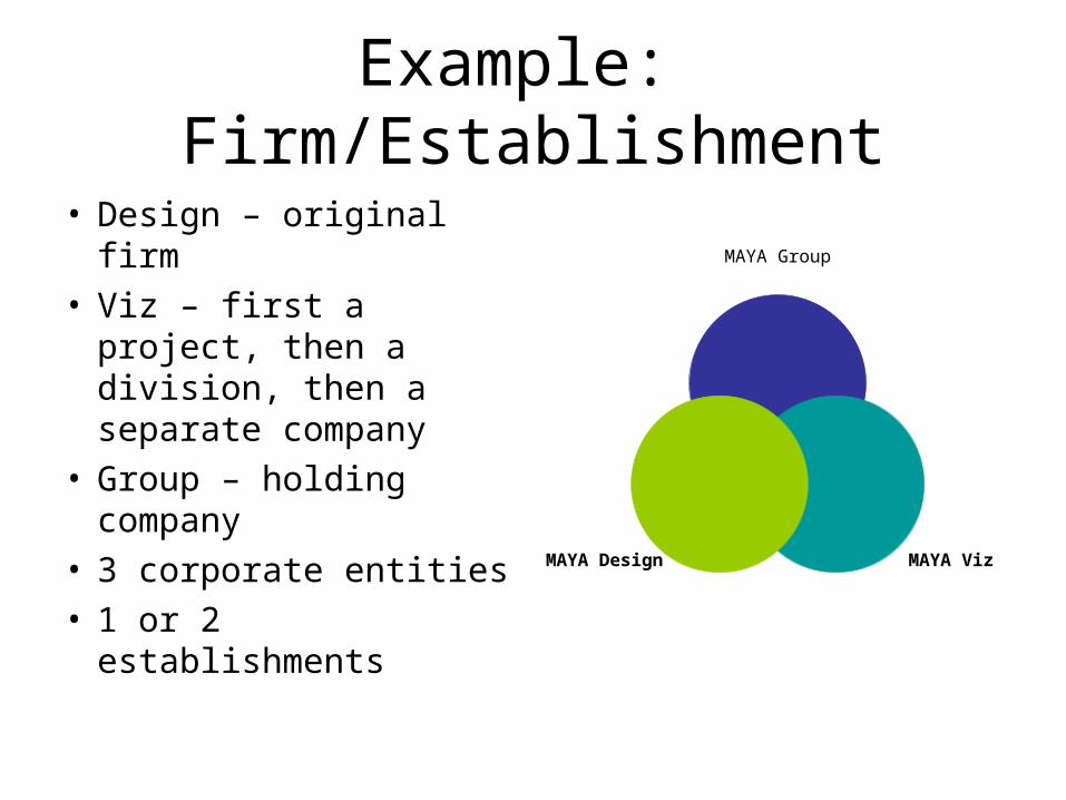
Example: Firm/Establishment

• Design – original firm• Viz – first a project,

then a division, then a separate company

• Group – holding company

• 3 corporate entities• 1 or 2 establishments

MAYA Group

MAYA VizMAYA Design

Combining Data

• Labor Force: – restricted to those more than 16 years old; doesn’t

include military or prison population; etc.

• Access to work– Jobs-to-the-labor force (jobs/LF)– why not Jobs-to-Population

• Dependency– Resident Employees-to-Population

• how many residents are working to support the population

Geography Issues

• Urban– All territory, population, and housing units located

within an urbanized area (UA) or an urban cluster (UC).

• core census block groups or blocks that have a population density of at least 1,000 people per square mile and

• surrounding census blocks that have an overall density of at least 500 people per square mile

• In addition, under certain conditions, less densely settled territory may be part of each UA or UC.

• Rural– All territory, population, and housing units located

outside of UAs and UCs.

Urban / Rural / Suburban

• Places, counties, metropolitan areas are often split between urban and rural territory. 

• For example, St. Mary's County, MD, is a predominantly rural county which contains a substantial urban population. 

• So what is a suburb?– Is it urban or rural or neither?

• States and counties typically don’t change• District, municipal, metropolitan and regional boundaries change

over time• www.ask.census.gov for information about geographic boundaries • Metropolitan areas

– The New England exception: NECTAs & NECMAs– If doing historical or trend analysis, MSA definitions may change – make

sure you’re talking about same consistent area over a specific time period

– Different kinds of MSAs– MSAs (metropolitan statistical area); – CSA (combined statistical area) – Macropolitan Statistical Area– Micropolitan Statistical Area

• FIPS State & County codes; also CBSA codes – both really helpful in ensuring that you’re pulling data from the same sources

Basic benchmarking can be helpfulAnnual Employment Growth, 1969-2000

-6.0%

-4.0%

-2.0%

0.0%

2.0%

4.0%

6.0%

1969

-197

0

1970

-197

1

1971

-197

2

1972

-197

3

1973

-197

4

1974

-197

5

1975

-197

6

1976

-197

7

1977

-197

8

1978

-197

9

1979

-198

0

1980

-198

1

1981

-198

2

1982

-198

3

1983

-198

4

1984

-198

5

1985

-198

6

1986

-198

7

1987

-198

8

1988

-198

9

1989

-199

0

1990

-199

1

1991

-199

2

1992

-199

3

1993

-199

4

1994

-199

5

1995

-199

6

1996

-199

7

1997

-199

8

1998

-199

9

1999

-200

0

Pittsburgh United States

Basic benchmarking can be helpfulEmployment Change, 1970-1993

0

100,000

200,000

300,000

400,000

500,000

600,000

700,000

800,000

San Diego Boise Tucson Fresno Memphis New Orleans Toledo Pittsburgh

The Scale Problem

-

20,000,000

40,000,000

60,000,000

80,000,000

100,000,000

120,000,000

140,000,000

160,000,000

180,000,000

1990 1991 1992 1993 1994 1995 1996 1997 1998 1999 2000 2001 2002 2003 2004

United States United States Metropolitan Portion

Pennsylvania Metropolitan Portion Pittsburgh, PA (MSA)

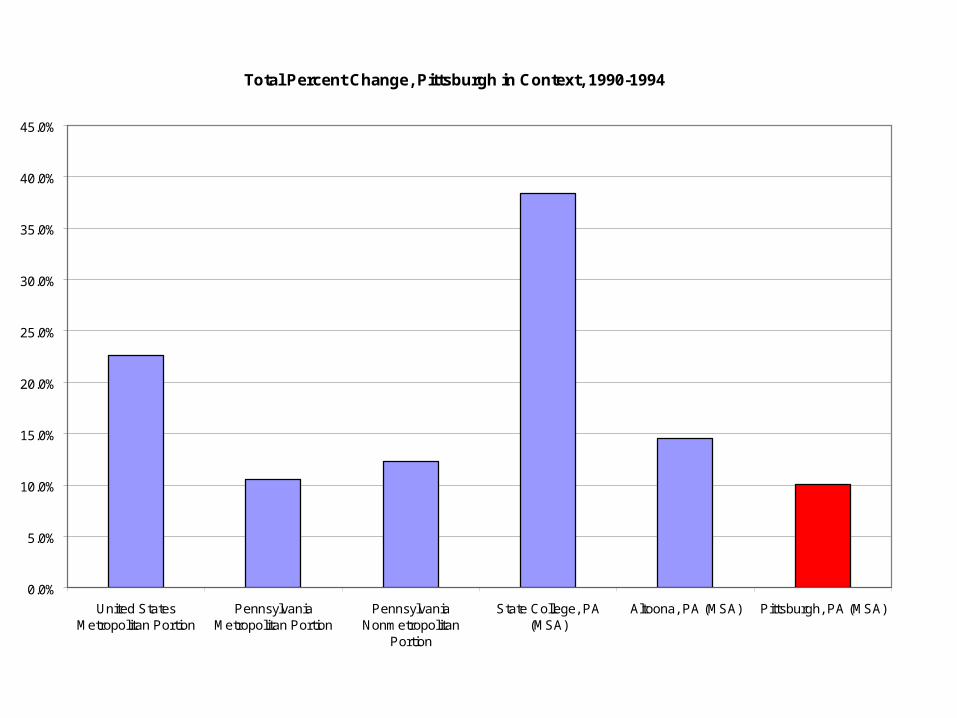
Total Percent Change, Pittsburgh in Context, 1990-1994

0.0%

5.0%

10.0%

15.0%

20.0%

25.0%

30.0%

35.0%

40.0%

45.0%

United StatesMetropolitan Portion

PennsylvaniaMetropolitan Portion

PennsylvaniaNonmetropolitan

Portion

State College, PA(MSA)

Altoona, PA (MSA) Pittsburgh, PA (MSA)

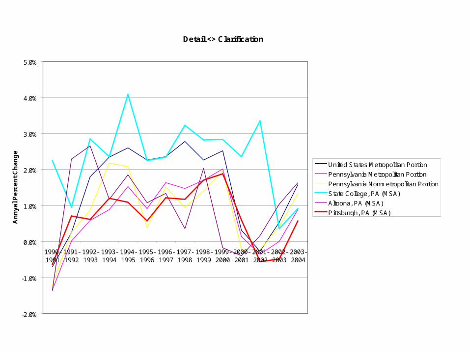
Detail <> Clarification

-2.0%

-1.0%

0.0%

1.0%

2.0%

3.0%

4.0%

5.0%

1990-1991

1991-1992

1992-1993

1993-1994

1994-1995

1995-1996

1996-1997

1997-1998

1998-1999

1999-2000

2000-2001

2001-2002

2002-2003

2003-2004

An

nya

l Per

cen

t C

han

ge

United States Metropolitan Portion

Pennsylvania Metropolitan Portion

Pennsylvania Nonmetropolitan Portion

State College, PA (MSA)

Altoona, PA (MSA)

Pittsburgh, PA (MSA)

Pittsburgh in Context - Different Averages

0.0%

0.5%

1.0%

1.5%

2.0%

2.5%

3.0%

Avg Pct Change 1 Avg Pct Change 2 AAGR

United States Metropolitan Portion

Pennsylvania Metropolitan Portion

Pennsylvania Nonmetropolitan Portion

State College, PA (MSA)

Altoona, PA (MSA)

Pittsburgh, PA (MSA)

Measures of Growth

• Linear Measure of Growth• Compound Measure of Growth• Percent Change in Population Growth between 1990 and

2000– 2000-1990 / 1990

• Average Annual Change– 2000-1990 / 1990; then that number divided by number of years

(how many years?)• Compound Average Growth Rate (CAGR)

– Compute annual change for every year and then take the average. More tedious computations.

– If have smooth procession of growth, Avg Annual vs CAGR will be pretty close. But, if have major ‘dip’ or ‘growth’ in one particular year, will get more precise number calculating CAGR vs Avg Annual

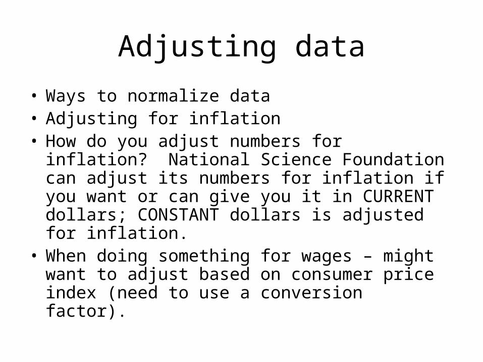
Adjusting data

• Ways to normalize data• Adjusting for inflation• How do you adjust numbers for inflation?

National Science Foundation can adjust its numbers for inflation if you want or can give you it in CURRENT dollars; CONSTANT dollars is adjusted for inflation.

• When doing something for wages – might want to adjust based on consumer price index (need to use a conversion factor).

Location Quotients

Loc

atio

n Q

uot

ien

t

Employment Growth

Important industries that may require attention

High

High

Low

Low

Important growth industries

Industries of little promise to local economy

Potential emerging industries

Total

Total

Industry

Industry

Region

Natio

n

Formula Interpretation

Using LQs• The Export Flaw

– Global production– Intermediate goods and end users

• Assumption Approach– Local = Government, Banking (is this still true?), – Utilities – Retail (The Amazon effect)

• Minimum Requirements Approach– The least a region needs to have

• Can use location quotient to get a sense of how many specialization industries a region has– Specialization –

• location quotients about 1.0 or 1.5• High LQ may be difficult to increase employment

– Diversification. • If all location quotients near or at a 1.0, will see the region mimicking the

national economy.

LQ quirks

• Sensitive to the size of the region and base• Sensitive to the level of industry

Industry Georgia -- Statewide

Atlanta-, GA MSA

NAICS 311 Food manufacturing 1.47 0.88

NAICS 31193 Flavoring syrup and concentrate manufacturing

ND ND

NAICS 3121 Beverage manufacturing 0.65 ND

NAICS 312111 Soft drink manufacturing 0.43 0.57

NAICS 484 Truck transportation 1.12

NAICS 484122 General freight trucking, long-distance

2.43

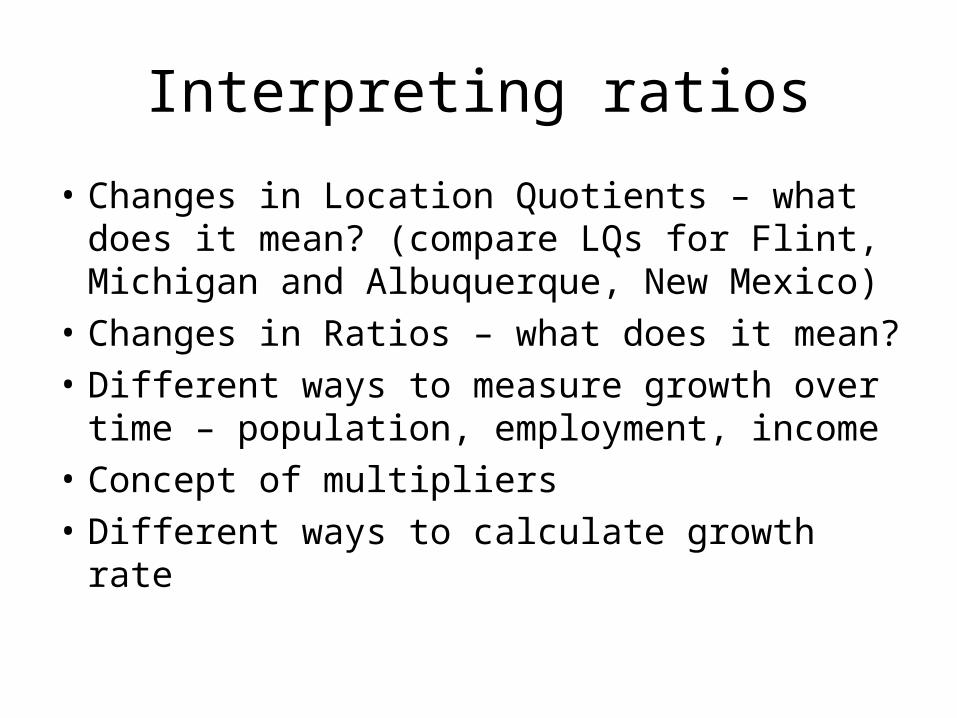
Interpreting ratios

• Changes in Location Quotients – what does it mean? (compare LQs for Flint, Michigan and Albuquerque, New Mexico)

• Changes in Ratios – what does it mean?

• Different ways to measure growth over time – population, employment, income

• Concept of multipliers

• Different ways to calculate growth rate

Finding Key Industries

Military (small & not growing industry)

StLGov (large, Ind. Decline – but does that matter, is this desirable)

Farm (small, ind. decline

Mfg (small, Ind decline)

Svc (lg, growth industry)

HighLQ

LowLQ

Low Growth High Growth

The Policy Map

Brooks and Krugman

Part 2