Big Data

Technologies

Big Data Technologies | Syllabus 1. Introduction to Big Data

1.1 Big data overview

1.2 Background of data analytics

1.3 Role of distributed system in big data

1.4 Role of data scientist

1.5 Current trend in big data analytics 2. Google file system

2.1 Architecture

2.2 Availability

2.3 Fault tolerance

2.4 Optimization of large scale data 3. Map Reduce Framework

3.1 Basics of functional programming

3.2 Fundamentals of functional programming

3.3 Real world problems modelling in functional style

3.4 Map reduce fundamentals

3.5 Data flow (Architecture)

3.6 Real world problems

3.7 Scalability goal

3.8 Fault tolerance

3.9 Optimization and data locality

3.10 Parallel efficiency of map reduce 4. NoSQL

4.1 Structured and unstructured data

4.2 Taxonomy of NOSQL implementation

4.3 Discussion of basic architecture of Hbase, Cassandra and MongoDb 5. Searching and indexing big data

5.1 Full text indexing and searching

5.2 Indexing with Lucene

5.3 Distributed searching with elastic search 6. Case study: Hadoop

6.1 Introduction to Hadoop environment

6.2 Data flow

6.3 Hadoop I/O

6.4 Query language of Hadoop

6.5 Hadoop and amazon cloud

Table of Contents

S.N. Chapter Name Page No.

1. Big data technologies 3-11

2. Google file system 12-28

3. Map Reduce framework 29-40

4. NOSQL 41-63

5. Searching and Indexing 64-71

6. Case Study: Hadoop 72-77

Chapter 1: Big Data Technologies

Introduction

Big data is a term applied to a new generation of software, applications, and system and

storage architecture.

It designed to provide business value from unstructured data.

Big data sets require advanced tools, software, and systems to capture, store, manage,

and analyze the data sets,

All in a timeframe big data preserves the intrinsic value of the data.

Big data is now applied more broadly to cover commercial environments.

Four distinct applications segments comprise the big data market.

Each with varying levels of need for performance and scalability.

The four big data segments are:

1) Design (engineering collaboration)

2) Discover (core simulation – supplanting physical experimentation) 3)

Decide (analytics).

4) Deposit (Web 2.0 and data warehousing)

Why big data?

Three trends disrupting the database status quo– Big Data, Big Users, and Cloud

Computing

Big Users: Not that long ago, 1,000 daily users of an application was a lot and 10,000 was

an extreme case. Today, with the growth in global Internet use, the increased number

of hour’s users spend online, and the growing popularity of smartphones and tablets, it's

not uncommon for apps to have millions of users a day.

Big Data: Data is becoming easier to capture and access through third parties such as

Facebook, D&B, and others. Personal user information, geo location data, social graphs,

user-generated content, machine logging data, and sensor-generated data are just a few

examples of the ever-expanding array of data being captured.

Cloud Computing: Today, most new applications (both consumer and business) use a

three-tier Internet architecture, run in a public or private cloud, and support large

numbers of users.

Who uses big data?

Facebook, Amazon, Google, Yahoo, New York Times, twitter and many more

Data analytics

Big data analytics is the process of examining large amounts of data of a variety of types.

Analytics and big data hold growing potential to address longstanding issues in critical

areas of business, science, social services, education and development. If this power is to

be tapped responsibly, organizations need workable guidance that reflects the realities

of how analytics and the big data environment work.

The primary goal of big data analytics is to help companies make better business

decisions.

Analyze huge volumes of transaction data as well as other data sources that may be left

untapped by conventional business intelligence (BI) programs.

Big data analytics can be done with the software tools commonly used as part of

advanced analytics disciplines.

Such as predictive analysis and data mining.

But the unstructured data sources used for big data analytics may not fit in traditional

data warehouses.

Traditional data warehouses may not be able to handle the processing demands posed

by big data.

The technologies associated with big data analytics include NoSQL databases, Hadoop

and MapReduce.

Known about these technologies form the core of an open source software framework

that supports the processing of large data sets across clustered systems.

big data analytics initiatives include

- internal data analytics skills

- high cost of hiring experienced analytics professionals,

- challenges in integrating Hadoop systems and data warehouses

Big Analytics delivers competitive advantage in two ways compared to the traditional

analytical model.

First, Big Analytics describes the efficient use of a simple model applied to volumes of

data that would be too large for the traditional analytical environment.

Research suggests that a simple algorithm with a large volume of data is more accurate

than a sophisticated algorithm with little data

The term “analytics” refers to the use of information technology to harness statistics,

algorithms and other tools of mathematics to improve decision-making.

Guidance for analytics must recognize that processing of data may not be linear.

May involve the use of data from a wide array of sources.

Principles of fair information practices may be applicable at different points in analytic

processing.

Guidance must be sufficiently flexible to serve the dynamic nature of analytics and the

richness of the data to which it is applied.

The power and promise of analytics

Big Data Analytics to Improve Network Security.

Security professionals manage enterprise system risks by controlling access to systems,

services and applications defending against external threats.

Protecting valuable data and assets from theft and loss.

Monitoring the network to quickly detect and recover from an attack.

Big data analytics is particularly important to network monitoring, auditing and recovery.

Business Intelligence uses big data and analytics for these purposes.

Reducing Patient Readmission Rates (Medical data)

Big data to address patient care issues and to reduce hospital readmission rates.

The focus on lack of follow-up with patients, medication management issues and

insufficient coordination of care.

Data is preprocessed to correct any errors and to format it for analysis.

Analytics to Reduce the Student Dropout Rate (Educational Data)

Analytics applied to education data can help schools and school systems better

understand how students learn and succeed.

Based on these insights, schools and school systems can take steps to enhance education

environments and improve outcomes.

Assisted by analytics, educators can use data to assess and when necessary re-organize

classes, identify students who need additional feedback or attention.

Direct resources to students who can benefit most from them.

The process of analytics

This knowledge discovery phase involves

Gathering data to be analyzed.

Pre-processing it into a format that can be used.

Consolidating (more certain) it for analysis, analyzing it to discover what it may reveal.

And interpreting it to understand the processes by which the data was analyzed and how

conclusions were reached.

Acquisition –(process of getting something)

Data acquisition involves collecting or acquiring data for analysis.

Acquisition requires access to information and a mechanism for gathering it.

Pre-processing –:

Data is structured and entered into a consistent format that can be analyzed.

Pre-processing is necessary if analytics is to yield trustworthy (able to trusted), useful

results.

Places it in a standard format for analysis.

Integration –:

Integration involves consolidating data for analysis.

Retrieving relevant data from various sources for analysis

Eliminating redundant data or clustering data to obtain a smaller representative sample.

Clean data into its data warehouse and further organizes it to make it readily useful for

research.

distillation into manageable samples

Analysis – Knowledge discovery involves

Searching for relationships between data items in a database, or exploring data in search

of classifications or associations.

Analysis can yield descriptions (where data is mined to characterize properties) or

predictions (where a model or set of models is identified that would yield predictions).

Analysis based on interpretation, organizations can determine whether and how to act

on them.

Data scientist

Data scientists include

Data capture and Interpretation

New analytical techniques

Community of Science

Perfect for group work

Teaching strategies

Data scientist requires wide range of skills

Business domain expertise and strong analytical skills

Creativity and good communications.

Knowledgeable in statistics, machine learning and data visualization

Able to develop data analysis solutions using modeling/analysis methods and languages

such as Map-Reduce, R, SAS, etc.

Adept at data engineering, including discovering and mashing/blending large amounts

of data.

Data scientists use an investigative computing platform

To bring un-modeled data.

Multi-structured data, into an investigative data store for experimentation.

Deal with unstructured, semi-structured and structured data from various source.

Data scientist helps broaden the business scope of investigative computing in three areas:

New sources of data – supports access to multi-structured data.

New and improved analysis techniques – enables sophisticated analytical processing of multi-

structured data using techniques such as Map-Reduce and in-database analytic functions.

Improved data management and performance – provides improved price/performance for

processing multi-structured data using non-relational systems such as Hadoop, relational

DBMSs, and integrated hardware/software.

Goal of data analytics is the role of data scientist

Recognize and reflect the two-phased nature of analytic processes.

Provide guidance for companies about how to establish that their use of data for

knowledge discovery is a legitimate business purpose.

Emphasize the need to establish accountability through an internal privacy program that

relies upon the identification and mitigation of the risks the use of data for analytics may

raise for individuals.

Take into account that analytics may be an iterative process using data from a variety of

sources.

Current trend in big data analytics

Iterative process (Discovery and Application) In general:

Analyze the unstructured data (Data analytics)

development of algorithm (Data analytics)

Data Scrub (Data engineer)

Present structured data (relationship, association)

Data refinement (Data scientist)

Process data using distributed engine. E.g. HDFS (S/W engineer) and write to No-SQL DB (Elastic search, Hbase, MangoDB, Cassandra, etc)

Visual presentation in Application s/w.

QC verification.

Client release.

Questions:

Explain the term "Big Data". How could you say that your organization suffers from Big Data

problem?

Big data are those data sets with sizes beyond the ability of commonly used software tools to

capture, curate, manage, and process the data within a tolerable elapsed time Big data is the

term for a collection of data sets so large and complex that it becomes difficult to process using

on-hand database management tools or traditional data processing applications.

Big Data is often defined along three dimensions- volume, velocity and variety.

Big data is data that can be manipulated (slices and diced) with massive speed.

Big data is the not the standard fare that we use, but the more complex and intricate

data sets.

Big data is the unification and integration of diverse data sets (kill the data ghettos).

Big data is based on much larger amount of data sets than what we're used to and how

they can be resolved with both speed and variety.

Big data extrapolates the information in a different (three dimensional) way.

Data sets grow in size in part because they are increasingly being gathered by ubiquitous

information-sensing mobile devices, aerial sensory technologies (remote sensing), software

logs, cameras, microphones, radio-frequency identification readers, and wireless sensor

networks. The world's technological per-capita capacity to store information has roughly

doubled every 40 months since the 1980s; as of 2012, every day 2.5 quintillion (2.5×1018) bytes

of data were created. As the data collection is increasing day by day, is difficult to work with

using most relational database management systems and desktop statistics and visualization

packages, requiring instead "massively parallel software running on tens, hundreds, or even

thousands of servers. The challenges include capture, duration, storage, search, sharing,

transfer, analysis, and visualization. So such large gathering of data suffers the organization

forces the need to big data management with distributed approach.

Explain the role of distributed system in Big Data. You can provide illustrations with your case

study or example if you like.

A distributed system is a collection of independent computers that appears to its users as a single

coherent system. A distributed system is one in which components located at networked

computers communicate and coordinate their actions only by passing messages. Distributed

system play an important role in managing the big data problems that prevails in today’s world.

In the distributed approach, data are placed in multiple machines and are made available to the

user as if they are in a single system. Distributed system makes the proper use of hardware and

resources in multiple location and multiple machines.

Example: How google manages data for search engines?

Advances in digital sensors, communications, computation, and storage have created huge

collections of data, capturing information of value to business, science, government, and society.

For example, search engine companies such as Google, Yahoo!, and Microsoft have created an

entirely new business by capturing the information freely available on the World Wide Web and

providing it to people in useful ways. These companies collect trillions of bytes of data every day.

Due to accumulation of large amount of data in the web every day, it becomes difficult to

manage the document in the centralized server. So to overcome the big data problems, search

engines companies like Google uses distributed server. A distributed search engine is a search

engine where there is no central server. Unlike traditional centralized search engines, work such

as crawling, data mining, indexing, and query processing is distributed among several peers in

decentralized manner where there is no single point of control. Several distributed servers are

set up in different location. Challenges of distributed approach like heterogeneity, Scalability,

openness and Security are properly managed and the information are made accessed to the user

from nearby located servers. The mirror servers performs different types of caching operation

as required. A system having a resource manager, a plurality of masters, and a plurality of slaves,

interconnected by a communications network. To distribute data, a master determined that a

destination slave of the plurality slaves requires data. The master then generates a list of slaves

from which to transfer the data to the destination slave. The master transmits the list to the

resource manager. The resource manager is configured to select a source slave from the list

based on available system resources. Once a source is selected by the resource manager, the

master receives an instruction from the resource manager to initiate a transfer of the data from

the source slave to the destination slave. The master then transmits an instruction to commence

the transfer.

Explain the implications of "Big Data" in the current renaissance of computing.

In 1965, Intel cofounder Gordon Moore observed that the number of transistors on an

integrated circuit had doubled every year since the microchip was invented. Data density has

doubled approximately every 18 months, and the trend is expected to continue for at least two

more decades. Moore's Law now extends to the capabilities of many digital electronic devices.

Year after year, we're astounded by the implications of Moore's Law — with each new version

or update bringing faster and smaller computing devices. Smartphones and tablets now enable

us to generate and examine significantly more content anywhere and at any time. The amount

of information has grown exponentially, resulting in oversized data sets known as Big Data. Data

growth has rendered traditional management tools and techniques impractical to produce

meaningful results quickly. Computation tasks that used to take minutes now take hours or

timeout altogether before completing. To tame Big Data, we need new and better methods to

extract actionable insights. According to recent studies, the world's population will produce and

replicate 1.8 zeta bytes (or 1.8 trillion gigabytes) of data in 2011 alone — an increase of nine

times the data produced five years ago. The number of files or records (such as photos, videos,

and e-mail messages) is projected to grow 75 times, while the staff tasked with managing this

information is projected to increase by only 1.5 times. Big data is likely to be increasingly part of

IT world. Computation of Big data is difficult to work with using most relational database

management systems and desktop statistics and visualization packages, requiring instead

"massively parallel software running on tens, hundreds, or even thousands of servers" Big data

results in moving to constant improvement in traditional DBMS technology as well as new

databases like NoSQL and their ability to handle larger amounts of data To overcome the

challenges of big data, several computing technology have been developed. Big Data technology

has matured to the extent that we're now able to produce answers in seconds or minutes —

results that once took hours or days or were impossible to achieve using traditional analytics

tools executing on older technology platforms. This ability allows modelers and business

managers to gain critical insights quickly.

Chapter 2: Google file system

Introduction

Google File System, a scalable distributed file system for large distributed data-intensive

applications.

Google File System (GFS) to meet the rapidly growing demands of Google’s data

processing needs.

GFS shares many of the same goals as other distributed file systems such as

performance, scalability, reliability, and availability.

GFS provides a familiar file system interface.

Files are organized hierarchically in directories and identified by pathnames.

Support the usual operations to create, delete, open, close, read, and write files.

Small as well as multi-GB files are common.

Each file typically contains many application objects such as web documents.

GFS provides an atomic append operation called record append. In a traditional write,

the client specifies the offset at which data is to be written.

Concurrent writes to the same region are not serializable.

GFS has snapshot and record append operations.

Google (snapshot and record append)

The snapshot operation makes a copy of a file or a directory.

Record append allows multiple clients to append data to the same file concurrently while

guaranteeing the atomicity of each individual client’s append.

It is useful for implementing multi-way merge results.

GFS consist of two kinds of reads: large streaming reads and small random reads.

In large streaming reads, individual operations typically read hundreds of KBs, more

commonly 1 MB or more.

A small random read typically reads a few KBs at some arbitrary offset.

Common goals of GFS

Performance

Reliability

Scalability

Availability

Other GFS concepts

Component failures are the norm rather than the exception.

File System consists of hundreds or even thousands of storage machines built from

inexpensive commodity parts.

Files are Huge. Multi-GB Files are common.

Each file typically contains many application objects such as web documents.

Append, Append, Append.

Most files are mutated by appending new data rather than overwriting existing data.

Co-Designing

Co-designing applications and file system API benefits overall system by increasing

flexibility.

Why assume hardware failure is the norm?

- It is cheaper to assume common failure on poor hardware and account for it,

rather than invest in expensive hardware and still experience occasional failure.

-

- The amount of layers in a distributed system (network, disk, memory, physical

connections, power, OS, application) mean failure on any could contribute to data

corruption.

GFS Assumptions

System built from inexpensive commodity components that fail

Modest number of files – expect few million and > 100MB size. Did not optimize for

smaller files.

2 kinds of reads – :

- large streaming read (1MB)

- small random reads (batch and sort)

High sustained bandwidth chosen over low latency

GFS Interface

GFS – familiar file system interface

Files organized hierarchically in directories, path names

Create, delete, open, close, read, write operations

Snapshot and record append (allows multiple clients to append simultaneously - atomic)

GFS Architecture (Analogy)

On a single machine file system:

An upper layer maintains the metadata

A lower ie disk stores the data in units called blocks

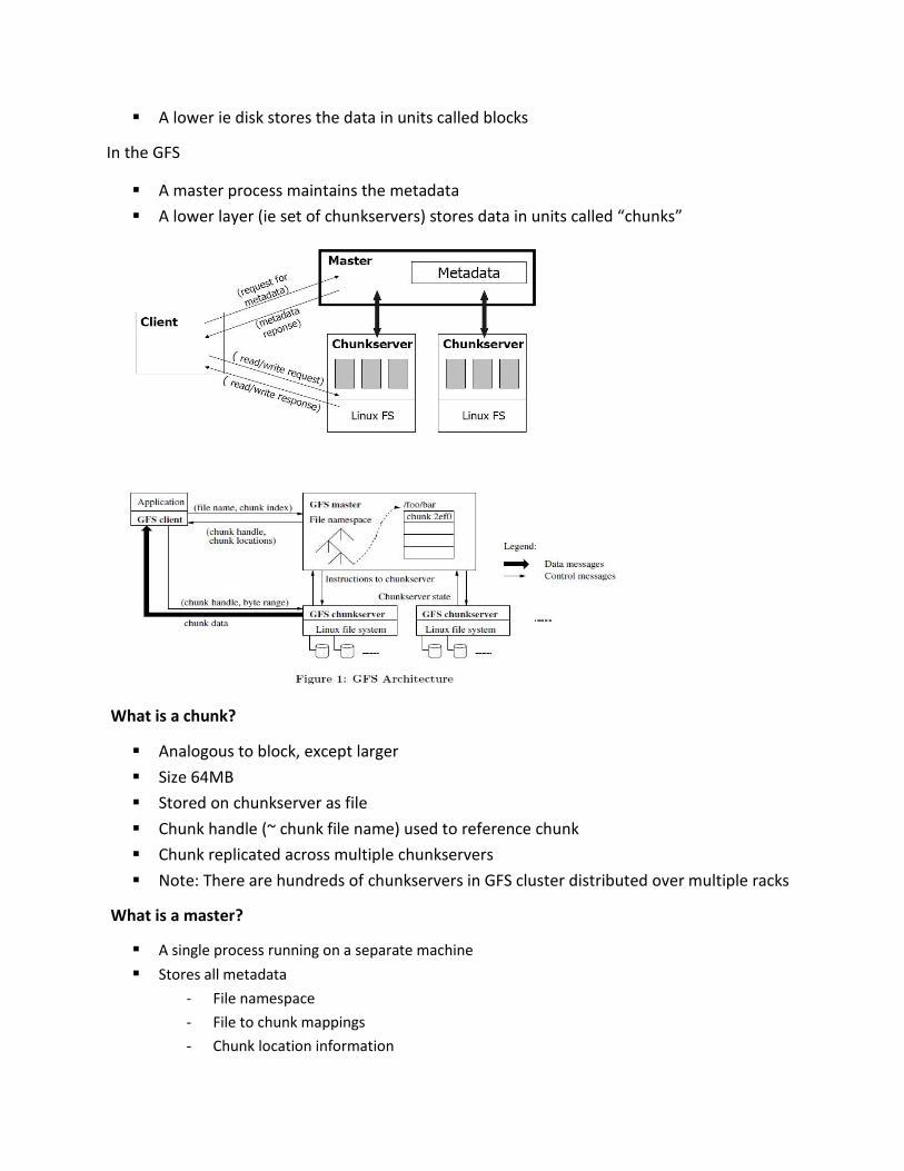
In the GFS

A master process maintains the metadata

A lower layer (ie set of chunkservers) stores data in units called “chunks”

What is a chunk?

Analogous to block, except larger

Size 64MB

Stored on chunkserver as file

Chunk handle (~ chunk file name) used to reference chunk

Chunk replicated across multiple chunkservers

Note: There are hundreds of chunkservers in GFS cluster distributed over multiple racks

What is a master?

A single process running on a separate machine

Stores all metadata

- File namespace

- File to chunk mappings

- Chunk location information

- Access control information

- Chunk version numbers

A GFS cluster consists of a single master and multiple chunk-servers and is accessed by multiple

clients. Each of these is typically a commodity Linux machine.

It is easy to run both a chunk-server and a client on the same machine.

As long as machine resources permit, it is possible to run flaky application code is acceptable.

Files are divided into fixed-size chunks.

Each chunk is identified by an immutable and globally unique 64 bit chunk assigned by the master

at the time of chunk creation.

Chunk-servers store chunks on local disks as Linux files, each chunk is replicated on multiple

chunk-servers.

The master maintains all file system metadata. This includes the namespace, access control

information, mapping from files to chunks, and the current locations of chunks.

It also controls chunk migration between chunk servers.

The master periodically communicates with each chunk server in Heart Beat messages to give it

instructions and collect its state.

Master <-> Server Communication

Master and chunkserver communicate regularly to obtain state:

Is chunkserver down?

Are there disk failures on chunkserver?

Are any replicas corrupted?

Which chunk replicas do chunkserver store?

Master sends instructions to chunkserver:

Delete existing chunk

Create new chunk

Serving requests:

Client retrieves metadata for operation form master

Read/write data flows between client and chunkserver

Single master is not bottleneck because its involvement with read/write operations is minimized

Read algorithm

Application originates the read request

GFS client translates the request from (filename, byte range) -> (filename, chunk, index), and

sends it to master

Master responds with chunk handle and replica locations (i.e chunkservers where replicas are

stored)

Client picks a location and sends the (chunk handle, byte range) request to that location

Chunkserver sends requested data to the client

Client forwards the data to the application

Write Algorithm

Application originates with request

GFS client translates request from (filename, data) -> (filename, chunk index) and sends

it to master

Master responds with chunk handle and (primary + secondary) replica locations

Client pushes write data to all locations. Data is stored in chunkservers’ internal buffer

Client sends write command to primary

Primary determines serial order for data instances stored in its buffer and writes the

instances in that order to the chunk

Primary sends order to the secondaries and tells them to perform the write

Secondaries responds to the primary

Primary responds back to the client

If write fails at one of chunkservers, client is informed and rewrites the write.

Record append algorithm

Important operations at Google:

- Merging results from multiple machines in one file

- Using file as producer – consumer queue

1. Application originates record append request

2. GFS client translates request and send it to master

3. Master responds with chunk handle and (primary + secondary) replica locations

4. Client pushes write data to all locations

5. Primary checks if record fits in specified chunk 6. If record does fit, then the primary: -

Pads the chunk

- Tells secondaries to do the same

- And informs the client

- Client then retries the append with the next chunk

7. If record fits, the primary:

- Appends the record

- Tells secondaries to do the same

- Receives responses from secondaries

- And sends final response to the client

GFS fault tolerance

Fast recovery: master and chunkservers are designed to restart restore state in a few

seconds

Chunk replication: across multiple machines, across multiple racks Master mechanisms:

- Log of all changes made to metadata

- Periodic checkpoints of the log

- Log and checkpoints replication on multiple machines

- Master state is replicated on multiple machines

- “Shadow” masters for reading data if “real” master is down

Data integrity

- Each chunk has an associated checksum

Metadata

Three types:

File and chunk namespaces

Mapping from files to chunks

Location of each chunk’s replicas

Instead of keeping track of chunk location info

- Poll: which chunkserver has which replica

- Master controls all chunk

placement

- Disks may go bad, chunkserver errors etc.

Consistency model

Write – data written at application specific offset

Record append – data appended automatically at least once at offset of GFS’s choosing

(Regular Append – write at offset, client thinks is EOF)

GFS

- Applies mutation to chunk in some order on all replicas

- Uses chunk version numbers to detect stale replicas

- Garbage collected, updated next time contact master

- Additional features – regular handshake master and chunkservers,

checksumming

- Data only lost if all replicas lost before GFS can react

Write control and data flow

Replica placement

GFS cluster distributed across many machine racks

Need communication across several network switches

Challenge to distribute data

Chunk replica

- Maximize data reliability

- Maximize network bandwidth utilization

Spread replicas across racks (survives even if entire rack offline)

R can exploit aggregate bandwidth of multiple racks

Re-replicate

- When number of replicas fall below goal:

- Chunkserver unavailable, corrupted etc.

- Replicate based on priority

Rebalance

- Periodically moves replicas for better disk space and load balancing

- Gradually fills up new chunkserver

- Removes replicas from chunkservers with below average space

Garbage collection

When delete file, file renamed to hidden name including delete timestamp

During regular scan of file namespace

- Hidden files removes if existed > 3 days

- Until then can be undeleted

- When removes, in memory metadata erased

- Orphaned chunks identified and erased

- With HeartBeat message, chunkserver/master exchange info about files, master

tells chunkserver about files it can delete, chunkserver free to delete

Advantages

- Simple, reliable in large scale distributed system

Chunk creation may success on some servers but not others

Replica deletion messages may be lost and resent

Uniform and dependable way to clean up replicas

- Merges storage reclamation with background activities of master

Done in batches

Done only when master free

- Delay in reclaiming storage provides against accidental deletion

Disadvantages

- Delay hinders user effort to fine tune usage when storage tight

- Applications that create/delete may not be able to reuse space right away

Expedite storage reclamation if file explicitly deleted again

Allow users to apply different replication and reclamation policies

Shadow master

Master replication

Replicated for reliability

One master remains in charge of all mutations and background activities

If fails, start instantly

If machine or disk mails, monitor outside GFS starts new master with replicated log

Clients only use canonical name of master

Shadow master

Read only access to file systems even when primary master down

Not mirrors, so may lag primary slightly

Enhance read availability for files not actively mutated

Shadow master read replica of operation log, applies same ssequence of changes to data

structures as primary does

Polls chunkserver at startup, monitors their status etc Depends only on primary for

replica location updates

Data integrity

Checksumming to detect corruption of stored data

Impractical to compare replicas across chunkservers to detec corruption

Divergent replicas may be legal

Chunk divided into 64 KB blocks, each with 32 bit checksum

Checksums stored in memory and persistently with logging

Before read, checksum

If problem, return error to requestor and reports to master

Requestor reads from replica, master clones chunk from other replica, delete bad replica

Most reads span multiple blocks, checksum small part of it

Checksum lookups done without I.O

Questions

With diagram explain general architecture of GFS.

Google organized the GFS into clusters of computers. A cluster is simply a network of computers.

Each cluster might contain hundreds or even thousands of machines. Within GFS clusters there

are three kinds of entities: clients, master servers and chunkservers. In the world of GFS, the

term "client" refers to any entity that makes a file request. Requests can range from retrieving

and manipulating existing files to creating new files on the system. Clients can be other

computers or computer applications. You can think of clients as the customers of the GFS. The

master server acts as the coordinator for the cluster. The master's duties include maintaining an

operation log, which keeps track of the activities of the master's cluster. The operation log helps

keep service interruptions to a minimum -- if the master server crashes, a replacement server

that has monitored the operation log can take its place. The master server also keeps track of

metadata, which is the information that describes chunks. The metadata tells the master server

to which files the chunks belong and where they fit within the overall file. Upon startup, the

master polls all the chunkservers in its cluster. The chunkservers respond by telling the master

server the contents of their inventories. From that moment on, the master server keeps track of

the location of chunks within the cluster. There's only one active master server per cluster at

any one time (though each cluster has multiple copies of the master server in case of a hardware

failure). That might sound like a good recipe for a bottleneck -- after all, if there's only one

machine coordinating a cluster of thousands of computers, wouldn't that cause data traffic

jams? The GFS gets around this sticky situation by keeping the messages the master server sends

and receives very small. The master server doesn't actually handle file data at all. It leaves that

up to the chunkservers. Chunkservers are the workhorses of the GFS. They're responsible for

storing the 64-MB file chunks. The chunkservers don't send chunks to the master server. Instead,

they send requested chunks directly to the client. The GFS copies every chunk multiple times

and stores it on different chunkservers. Each copy is called a replica. By default, the GFS makes

three replicas per chunk, but users can change the setting and make more or fewer replicas if

desired.

Explain the control flow of write mutation with diagram.

A mutation is an operation that changes the contents or metadata of a chunk such as a write or

an append operation. Each mutation is performed at all the chunk’s replicas. We use leases to

maintain a consistent mutation order across replicas. The master grants a chunk lease to one of

the replicas, which we call the primary. The primary picks a serial order for all mutations to the

chunk. All replicas follow this order when applying mutations. Thus, the global mutation order

is defined first by the lease grant order chosen by the master, and within a lease by the serial

numbers assigned by the primary.

The lease mechanism is designed to minimize management overhead at the master. A lease has

an initial timeout of 60 seconds. However, as long as the chunk is being mutated, the primary

can request and typically receive extensions from the master indefinitely. These extension

requests and grants are piggybacked on the Heart Beat messages regularly exchanged between

the master and all chunkservers. The master may sometimes try to revoke a lease before it

expires (e.g., when the master wants to disable mutations on a file that is being renamed). Even

if the master loses communication with a primary, it can safely grant a new lease to another

replica after the old lease expires.

We illustrate this process by following the control flow of a write through these numbered steps:

1. The client asks the master which chunkserver holds the current lease for the chunk and

the locations of the other replicas. If no one has a lease, the master grants one to a replica

it chooses (not shown).

2. The master replies with the identity of the primary and the locations of the other

(secondary) replicas. The client caches this data for future mutations. It needs to contact

the master again only when the primary becomes unreachable or replies that it no longer

holds a lease.

3. The client pushes the data to all the replicas. A client can do so in any order. Each

chunkserver will store the data in an internal LRU buffer cache until the data is used or

aged out. By decoupling the data flow from the control flow, we can improve

performance

by scheduling the expensive data flow based on the network topology regardless of

which chunkserver is the primary.

4. Once all the replicas have acknowledged receiving the data, the client sends a write

request to the primary. The request identifies the data pushed earlier to all of the

replicas. The primary assigns consecutive serial numbers to all the mutations it receives,

possibly from multiple clients, which provides the necessary serialization. It applies the

mutation to its own local state in serial number order.

5. The primary forwards the write request to all secondary replicas. Each secondary replica

applies mutations in the same serial number order assigned by the primary.

6. The secondaries all reply to the primary indicating that they have completed the

operation. 7. The primary replies to the client. Any errors encountered at any of the

replicas are reported to the client. In case of errors, the write may have succeeded at the

primary and an arbitrary subset of the secondary replicas. (If it had failed at the primary,

it would not have been assigned a serial number and forwarded.) The client request is

considered to have failed, and the modified region is left in an inconsistent state. Our

client code handles such errors by retrying the failed mutation. It will make a few

attempts at steps (3) through (7) before falling back to a retry from the be-ginning of the

write.

If a write by the application is large or straddles a chunk boundary, GFS client code breaks it

down into multiple write operations. They all follow the control flow described above but may

be interleaved with and overwritten by con-current operations from other clients. Therefore,

the shared file region may end up containing fragments from different clients, although the

replicas will be identical because the individual operations are completed successfully in the

same order on all replicas. This leaves the file region in consistent but undefined state.

Why do we have single master in GFS managing millions of chunkservers? What are done to

manage it without overloading single master?

Having a single master vastly simplifies the design of GFS and enables the master to make

sophisticated chunk placement and replication decisions using global knowledge. However, the

involvement of master in reads and writes must be minimized so that it does not become a

bottleneck. Clients never read and write file data through the master. Instead, a client asks the

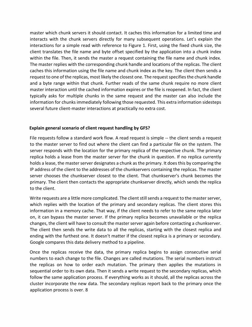
master which chunk servers it should contact. It caches this information for a limited time and

interacts with the chunk servers directly for many subsequent operations. Let’s explain the

interactions for a simple read with reference to Figure 1. First, using the fixed chunk size, the

client translates the file name and byte offset specified by the application into a chunk index

within the file. Then, it sends the master a request containing the file name and chunk index.

The master replies with the corresponding chunk handle and locations of the replicas. The client

caches this information using the file name and chunk index as the key. The client then sends a

request to one of the replicas, most likely the closest one. The request specifies the chunk handle

and a byte range within that chunk. Further reads of the same chunk require no more client

master interaction until the cached information expires or the file is reopened. In fact, the client

typically asks for multiple chunks in the same request and the master can also include the

information for chunks immediately following those requested. This extra information sidesteps

several future client-master interactions at practically no extra cost.

Explain general scenario of client request handling by GFS?

File requests follow a standard work flow. A read request is simple -- the client sends a request

to the master server to find out where the client can find a particular file on the system. The

server responds with the location for the primary replica of the respective chunk. The primary

replica holds a lease from the master server for the chunk in question. If no replica currently

holds a lease, the master server designates a chunk as the primary. It does this by comparing the

IP address of the client to the addresses of the chunkservers containing the replicas. The master

server chooses the chunkserver closest to the client. That chunkserver's chunk becomes the

primary. The client then contacts the appropriate chunkserver directly, which sends the replica

to the client.

Write requests are a little more complicated. The client still sends a request to the master server,

which replies with the location of the primary and secondary replicas. The client stores this

information in a memory cache. That way, if the client needs to refer to the same replica later

on, it can bypass the master server. If the primary replica becomes unavailable or the replica

changes, the client will have to consult the master server again before contacting a chunkserver.

The client then sends the write data to all the replicas, starting with the closest replica and

ending with the furthest one. It doesn't matter if the closest replica is a primary or secondary.

Google compares this data delivery method to a pipeline.

Once the replicas receive the data, the primary replica begins to assign consecutive serial

numbers to each change to the file. Changes are called mutations. The serial numbers instruct

the replicas on how to order each mutation. The primary then applies the mutations in

sequential order to its own data. Then it sends a write request to the secondary replicas, which

follow the same application process. If everything works as it should, all the replicas across the

cluster incorporate the new data. The secondary replicas report back to the primary once the

application process is over. 8

At that time, the primary replica reports back to the client. If the process was successful, it ends

here. If not, the primary replica tells the client what happened. For example, if one secondary

replica failed to update with a particular mutation, the primary replica notifies the client and

retries the mutation application several more times. If the secondary replica doesn't update

correctly, the primary replica tells the secondary replica to start over from the beginning of the

write process. If that doesn't work, the master server will identify the affected replica as garbage.

Why do we have large and fixed sized Chunks in GFS? What can be demerits of that design?

Chunks size is one of the key design parameters. In GFS it is 64 MB, which is much larger than

typical file system blocks sizes. Each chunk replica is stored as a plain Linux file on a chunkserver

and is extended only as needed.

Some of the reasons to have large and fixed sized chunks in GFS are as follows:

1. It reduces clients’ need to interact with the master because reads and writes on the same

chunk require only one initial request to the master for chunk location information. The

reduction is especially significant for the workloads because applications mostly read and

write large files sequentially. Even for small random reads, the client can comfortably

cache all the chunk location information for a multi-TB working set.

2. Since on a large chunk, a client is more likely to perform many operations on a given

chunk, it can reduce network overhead by keeping a persistent TCP connection to the

chunkserver over an extended period of time.

3. It reduces the size of the metadata stored on the master. This allows us to keep the

metadata in memory, which in turn brings other advantages.

Demerits of this design are mentioned below:

1. Lazy space allocation avoids wasting space due to internal fragmentation.

2. Even with lazy space allocation, a small file consists of a small number of chunks, perhaps

just one. The chunkservers storing those chunks may become hot spots if many clients

are accessing the same file. In practice, hot spots have not been a major issue because

the applications mostly read large multi-chunk files sequentially. To mitigate it,

replication and allowance to read from other clients can be done.

What are implications of having write and read lock in file operations. Explain for File creation

and snapshot operations.

GFS applications can accommodate the relaxed consistency model with a few simple techniques

already needed for other purposes: relying on appends rather than overwrites, checkpointing,

and writing self-validating, self-identifying records. Practically all the applications mutate files by

appending rather than overwriting. In one typical use, a writer generates a file from beginning

to end. It atomically renames the file to a permanent name after writing all the data, or

periodically checkpoints how much has been successfully written. Checkpoints may also include

applicationlevel checksums. Readers verify and process only the file region up to the last

checkpoint, which is known to be in the defined state. Regardless of consistency and

concurrency issues, this approach has served us well. Appending is far more efficient and more

resilient to application failures than random writes. Checkpointing allows writers to restart

incrementally and keeps readers from processing successfully written file data that is still

incomplete from the application’s perspective. In the other typical use, many writers

concurrently append to a file for merged results or as a producer-consumer queue. Record

appends append-at-least-once semantics preserves each writer’s output. Readers deal with the

occasional padding and duplicates as follows. Each record prepared by the writer contains extra

information like checksums so that its validity can be verified. A reader can identify and discard

extra padding and record fragments using the checksums. If it cannot tolerate the occasional

duplicates (e.g., if they would trigger non-idempotent operations), it can filter them out using

unique identifiers in the records, which are often needed anyway to name corresponding

application entities such as web documents. These functionalities for record I/O (except

duplicate removal) are in library code shared by the applications and applicable to other file

interface implementations at Google. With that, the same sequence of records, plus rare

duplicates, is always delivered to the record reader.

Like AFS, Google use standard copy-on-write techniques to implement snapshots. When the

master receives a snapshot request, it first revokes any outstanding leases on the chunks in the

files it is about to snapshot. This ensures that any subsequent writes to these chunks will require

an interaction with the master to find the lease holder. This will give the master an opportunity

to create a new copy of the chunk first. After the leases have been revoked or have expired, the

master logs the operation to disk. It then applies this log record to its in-memory state by

duplicating the metadata for the source file or directory tree. The newly created snapshot files

point to the same chunks as the source files. The first time a client wants to write to a chunk C

after the snapshot operation, it sends a request to the master to find the current lease holder.

The master notices that the Reference count for chunk C is greater than one. It defers replying

to the client request and instead picks a new chunk handle C’. It then asks each chunkserver that

has a current replica of C to create a new chunk called C’. By creating the new chunk on the same

chunkservers as the original, it ensure that the data can be copied locally, not over the network

(the disks are about three times as fast as the 100 Mb Ethernet links). From this point, request

handling is no different from that for any chunk: the master grants one of the replicas a lease on

the new chunk C’ and replies to the client, which can write the chunk normally, not knowing that

it has just been created from an existing chunk.

Chapter 3: Map-Reduce Framework

Map-Reduce is a programming model designed for processing large volumes of data in

parallel by dividing the work into a set of independent tasks.

Map-Reduce programs are written in a particular style influenced by functional

programming constructs, specifically idioms for processing lists of data.

This module explains the nature of this programming model and how it can be used to

write programs which run in the Hadoop environment.

Map-Reduce

sort/merge based distributed processing

Best for batch- oriented processing

Sort/merge is primitive

Operates at transfer rate (Process + data clusters)

Simple programming metaphor:

- – input | map | shuffle | reduce > output

- – cat * | grep | sort | uniq c > file

Pluggable user code runs in generic reusable framework

- log processing,

- web search indexing

- SQL like queries in PIG

Distribution & reliability

Handled by framework - transparency

MR Model

Map()

Process a key/value pair to generate intermediate key/value pairs

Reduce()

Merge all intermediate values associated with the same key

Users implement interface of two primary methods:

1. Map: (key1, val1) → (key2, val2)

2. Reduce: (key2, [val2]) → [val3]

Map - clause group-by (for Key) of an aggregate function of SQL

Reduce - aggregate function (e.g., average) that is computed over all the rows with the

same group-by attribute (key).

Application writer specifies

A pair of functions called Map and Reduce and a set of input files and submits the job

Workflow

- Input phase generates a number of FileSplits from input files (one per Map task)

- The Map phase executes a user function to transform input kev-pairs into a new set of

kev-pairs

- The framework sorts & Shuffles the kev-pairs to output nodes

- The Reduce phase combines all kev-pairs with the same key into new kevpairs

- The output phase writes the resulting pairs to files

All phases are distributed with many tasks doing the work

- Framework handles scheduling of tasks on cluster

- Framework handles recovery when a node fails

Data distribution

Input files are split into M pieces on distributed file system - 128 MB

blocks

Intermediate files created from map tasks are written to local disk

Output files are written to distributed file system

Assigning tasks

Many copies of user program are started

Tries to utilize data localization by running map tasks on machines with data

One instance becomes the Master

Master finds idle machines and assigns them tasks

Execution

Map workers read in contents of corresponding input partition

Perform user-defined map computation to create intermediate <key,value> pairs

Periodically buffered output pairs written to local disk

Reduce

Reduce workers iterate over ordered intermediate data

Each unique key encountered – values are passed to user's reduce function eg.

<key, [value1, value2,..., valueN]>

Output of user's reduce function is written to output file on global file system When all tasks have completed, master wakes up user program

Data flow

Input, final output are stored on a distributed file system

Scheduler tries to schedule map tasks “close” to physical storage location of input data

Intermediate results are stored on local FS of map and reduce workers Output is often

input to another map reduce task

Co-ordination

Master data structures

- Task status: (idle, in-progress, completed)

- Idle tasks get scheduled as workers become available

- When a map task completes, it sends the master the location and sizes of its R

intermediate files, one for each reducer

- Master pushes this info to reducers

Master pings workers periodically to detect failures

Failures

Map worker failure

- Map tasks completed or in-progress at worker are reset to idle

- Reduce workers are notified when task is rescheduled on another worker

Reduce worker failure

- Only in-progress tasks are reset to idle

Master failure

- MapReduce task is aborted and client is notified

Combiners

Can map task will produce many pairs of the form (k,v1), (k,v2), … for the same key k E.g.,

popular words in Word Count

have network time by pre-aggregating at mapper

- combine(k1, list(v1)) v2

- Usually same as reduce function

Works only if reduce function is commutative and associative

Partition function

Inputs to map tasks are created by contiguous splits of input file

For reduce, we need to ensure that records with the same intermediate key end up at

the same worker

System uses a default partition function e.g., hash(key) mod R

Sometimes useful to override

Execution summary

How is this distributed?

- Partition input key/value pairs into chunks, run map() tasks in parallel

- After all map()s are complete, consolidate all emitted values for each unique emitted

key - Now partition space of output map keys, and run reduce() in parallel If map()

or reduce() fails, reexecute!

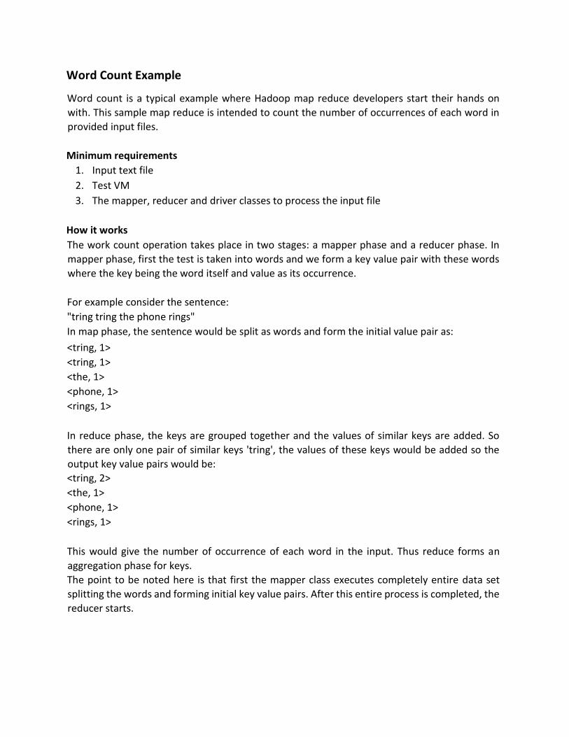
Word Count Example

Word count is a typical example where Hadoop map reduce developers start their hands on

with. This sample map reduce is intended to count the number of occurrences of each word in

provided input files.

Minimum requirements

1. Input text file

2. Test VM

3. The mapper, reducer and driver classes to process the input file

How it works

The work count operation takes place in two stages: a mapper phase and a reducer phase. In

mapper phase, first the test is taken into words and we form a key value pair with these words

where the key being the word itself and value as its occurrence.

For example consider the sentence:

"tring tring the phone rings"

In map phase, the sentence would be split as words and form the initial value pair as:

<tring, 1>

<tring, 1>

<the, 1>

<phone, 1>

<rings, 1>

In reduce phase, the keys are grouped together and the values of similar keys are added. So

there are only one pair of similar keys 'tring', the values of these keys would be added so the

output key value pairs would be:

<tring, 2>

<the, 1>

<phone, 1>

<rings, 1>

This would give the number of occurrence of each word in the input. Thus reduce forms an

aggregation phase for keys.

The point to be noted here is that first the mapper class executes completely entire data set

splitting the words and forming initial key value pairs. After this entire process is completed, the

reducer starts.

Questions:

List components in a basic MapReduce job. Explain with diagram how does the data flow

through Hadoop MapReduce.

Components in Basic MapReduce Job

MapReduce is a programming model and an associated implementation for processing and

generating large data sets. Programs written in this functional style of MapReduce are

automatically parallelized and executed on a large cluster of commodity machines. In a basic

MapReduce job, it consists of the following four components:

Input

Mapper

Reducer

Output

The input data is usually large and the computations have to be distributed across hundreds or

thousands of machines in order to finish in a reasonable amount of time. A MapReduce job

usually splits the input data-set into independent pieces usually 16 MB to 64 MB per piece which

are processed by the mapper component in a completely parallel manner as key/value pairs to

generate a set of intermediate key/value pairs. The reducer component merges all the

intermediate values associated with the same intermediate key and provided as output files.

Typically both the input and the output of the job are stored in a file-system. In a MapReduce

job, a special program called master assigns mapper or reducer tasks to rest of the idle workers.

Although, the basic MapReduce job consists of the above components, followings are also the

useful extensions:

Partitioner – partitions the data into specified number of reduce tasks/output files

Combiner – does partial merging of the data before sending over the network

Data Flow through Hadoop MapReduce

Hadoop MapReduce runs the job by dividing it into tasks, of which there are two types: map

tasks and reduce tasks. There are two types of nodes that control the job execution process: a

jobtracker (master) and a number of tasktrackers (workers). The jobtracker coordinates all the

jobs run on the system by scheduling tasks to run on tasktrackers. Hadoop divides the input to

a MapReduce job into fixed-size pieces called input splits, or just splits. Hadoop creates one map

task for each split, which runs the user-defined map function for each record in the split. Having

many splits means the time taken to process each split is small compared to the time to process

the whole input. On the other hand, if splits are too small, then the overhead of managing the

splits and of map task creation begins to dominate the total job execution time. Hadoop does its

best to run the map task on a node where the input data resides in HDFS. This is called the data

locality optimization. That’s why the optimal split size is the same as the block size so that the

largest size of input can be guaranteed to be stored on a single node. Map tasks write their

output to local disk, not to HDFS. The reducer(s) is fed by the mapper outputs. The output of the

reducer is normally stored in HDFS for reliability. The whole data flow with a single reduce task

is illustrated in Figure 2-2. The dotted boxes indicate nodes, the light arrows show data transfers

on a node, and the heavy arrows show data transfers between nodes. The number of reduce

tasks is not governed by the size of the input, but is specified independently.

How is MapReduce library designed to tolerate different machines (map/reduce nodes) failure

while executing MapReduce job?

Since the MapReduce library is designed to help process very large amounts of data using

hundreds or thousands of machines, the library must tolerate machine failures gracefully. The

MapReduce library is resilient to the large-scale failures in workers as well as master which is

well - explained below:

Worker(s) Failure

The master pings every worker periodically. If no response is received from a worker in a certain

amount of time, the master marks the worker as failed. Any map tasks completed by the worker

are reset back to their initial idle state, and therefore become eligible for scheduling on other

workers. Similarly, any map task or reduce task in progress on a failed worker is also reset to idle

and becomes eligible for rescheduling. Completed map tasks are re-executed on a failure

because their output is stored on the local disk(s) of the failed machine and is therefore

inaccessible. Completed reduce tasks do not need to be re-executed since their output is stored

in a global file system.

Master Failure

It is easy to make the master write periodic checkpoints of the master data structures – state &

identity of the worker machines. If the master task dies, a new copy can be started from the last

checkpointed state. However, given that there is only a single master, its failure is unlikely;

therefore, Jeffrey Dean & S. Ghemawat suggest to abort the MapReduce computation if the

master fails. Clients can check for this condition and retry the MapReduce operation if they

desire. Thus, in summary, the MapReduce library is/must be highly resilient towards the

different failures in map as well as reduce tasks distributed over several machines/nodes.

What is Straggler Machine? Describe how map reduce framework handles the straggler machine.

Straggler machine is a machine that takes an unusually long time to complete one of the last few map or reduce tasks in the computation. Stragglers can arise for a whole host of reasons. Stragglers are usually generated due to the variation in the CPU availability, network traffic or IO contention. Since a job in Hadoop environment does not finish until all Map and Reduce tasks are finished, even small number of stragglers can largely deteriorate the overall response time for the job. It is therefore essential for Hadoop to find stragglers and run a speculative copy to ensure lower response times. Earlier the detection of the stragglers, better is the overall response time for the job. The detection of stragglers needs to be accurate, since the speculative copies put up an overhead on the available resources. In homogeneous environment Hadoop’s native scheduler executes speculative copies by comparing the progresses of similar tasks. It determines the tasks with low progresses to be the stragglers and depending upon the availability of open slots, it duplicates a task copy. So map reduce can handle straggler more easily in homogenous environment. However this approach lead to performance degradation in heterogeneous environments. To deal with the stragglers in heterogeneous environment different approaches like LATE (Longest Approximate Time to End) and MonTool exists. But to the deficiencies in LATE, MonTool is widely used. In MonTool track disk and network system calls are tracked for the analysis. MonTool is designed on the underlying assumption that all map or reduce tasks work upon similar sized workloads and access data in a similar pattern. This assumption is fairly valid for map tasks which read equal amount of data and execute same operations on the data. Although the data size read by reduce tasks may be different for each

task, the data access pattern would still remain the same. We therefore track the data usage pattern by individual tasks by logging following system calls:

1. Data read from disk

2. Data write to disk

3. Data read from network

4. Data write on network

A potential straggler would access the data at a rate slower than its peers and this can be

validated by the system call pattern. So this strategy would definitely track straggler earlier on.

Also, as the data access pattern is not approximate, one can expect that this mechanism would

be more accurate Furthermore, MonTool runs a daemon on each slave node which periodically

sends monitoring information to the master node. Further, the master can query slaves to

understand the causes for the task delays.

Describe with an example how you would achieve a total order partitioning in MapReduce.

Partitioners are application code that define how keys are assigned to reduce. In Map Reduce

users specify the number of reduce tasks/output files that they desire (R). Data gets partitioned

across these tasks using a partitioning function on the intermediate key. A default partitioning

function is provided that uses hashing (e.g. hash (key) mod R).This tends to result in fairly

wellbalanced partitions. In some cases, however, it is useful to partition data by some other

function of the key. For example, sometimes the output keys are URLs, and we want all entries

for a single host to end up in the same output file. To support situations like this, the user of the

Map Reduce library can provide a special partitioning function. For example, using hash

(Hostname (urlkey)) mod R as the partitioning function causes all URLs from the same host to

end up in the same output file. Within a given partition, the intermediate key/value pairs are

processed in increasing key order. This ordering guarantee makes it easy to generate a sorted

output file per partition, which is useful when the output file format needs to support efficient

random access lookups by key, or users of the output find it convenient to have the data sorted.

What is the combiner function? Explain its purpose with suitable example.

Combiner is a user specified function that does partial merging of the data before it is sent over

the network. In some cases, there is significant repetition in the inter-mediate keys produced by

each map task. For example in the word counting example in word frequencies tend to follow a

Zipf distribution and each map task will produce hundreds or thousands of records of the form

<the, 1>. All of these counts will be sent over the network to a single reduce task and then added

together by the Reduce function to produce one number. So to decentralize the count of reduce,

user are allowed to specify an optional Combiner function that does partial merging of this data

before it is sent over the network. The Combiner function is executed on each machine that

performs a map task. No extra effort is necessary to implement the combiner function since the

same code is used to implement both the combiner and the reduce functions.

Chapter 4: NOSQL

The inter-related mega trends

Big data

Big users

Cloud computing

are driving the adoption of NoSQL technology

Why NO-SQL ?

Google, Amazon, Facebook, and LinkedIn were among the first companies to discover

the serious limitations of relational database technology for supporting these new

application requirements.

Commercial alternatives didn’t exist, so they invented new data management

approaches themselves. Their pioneering work generated tremendous interest because

a growing number of companies faced similar problems.

Open source NoSQL database projects formed to leverage the work of the pioneers, and

commercial companies associated with these projects soon followed.

1,000 daily users of an application was a lot and 10,000 was an extreme case.

Today, most new applications are hosted in the cloud and available over the Internet,

where they must support global users 24 hours a day, 365 days a year.

More than 2 billion people are connected to the Internet worldwide – and the amount

time they spend online each day is steadily growing – creating an explosion in the

number of concurrent users.

Today, it’s not uncommon for apps to have millions of different users a day.

New Generation Databases mostly addressing some of the points

being non-relational

distributed

Opensource

and horizontal scalable.

Multi-dimensional rather than 2-D (relational)

The movement began early 2009 and is growing rapidly.

Characteristics:

schema-free

Decentralized Storage System easy replication support Simple API, etc.

Introduction

the term means Not Only SQL

It's not SQL and it's not relational. NoSQL is designed for distributed data stores for very

large scale data needs.

In a NoSQL database, there is no fixed schema and no joins. Scaling out refers to

spreading the load over many commodity systems. This is the component of NoSQL that

makes it an inexpensive solution for large datasets.

Application needs have been changing dramatically, due in large part to three trends:

growing numbers of users that applications must support growth in the volume and

variety of data that developers must work with; and the rise of cloud computing.

NoSQL technology is rising rapidly among Internet companies and the enterprise

because it offers data management capabilities that meet the needs of modern

application:

Greater ability to scale dynamically to support more users and data

Improved performance to satisfy expectations of users wanting highly responsive

applications and to allow more complex processing of data.

NoSQL is increasingly considered available alternative to relational databases, and

should be considered particularly for interactive web and mobile applications.

Examples

Cassandra, MongoDB, Elastic search, Hbase, CouchDB, StupidDB etc

Querying NO-SQL

The question of how to query a NoSQL database is what most developers are interested

in. After all, data stored in a huge database doesn't do anyone any good if you can't

retrieve and show it to end users or web services. NoSQL databases do not provide a high

level declarative query language like SQL. Instead, querying these databases is datamodel

specific.

Many of the NoSQL platforms allow for RESTful interfaces to the data. Other offer query

APIs. There are a couple of query tools that have been developed that attempt to query

multiple NoSQL databases. These tools typically work accross a single NoSQL category.

One example is SPARQL. SPARQL is a declarative query specification designed for graph

databases. Here is an example of a SPARQL query that retrieves the URL of a particular

blogger (courtesy of IBM):

PREFIX foaf: <http://xmlns.com/foaf/0.1/>

SELECT ?url

FROM <bloggers.rdf>

WHERE {

?contributor foaf:name "Jon Foobar" .

?contributor foaf:weblog ?url .

}

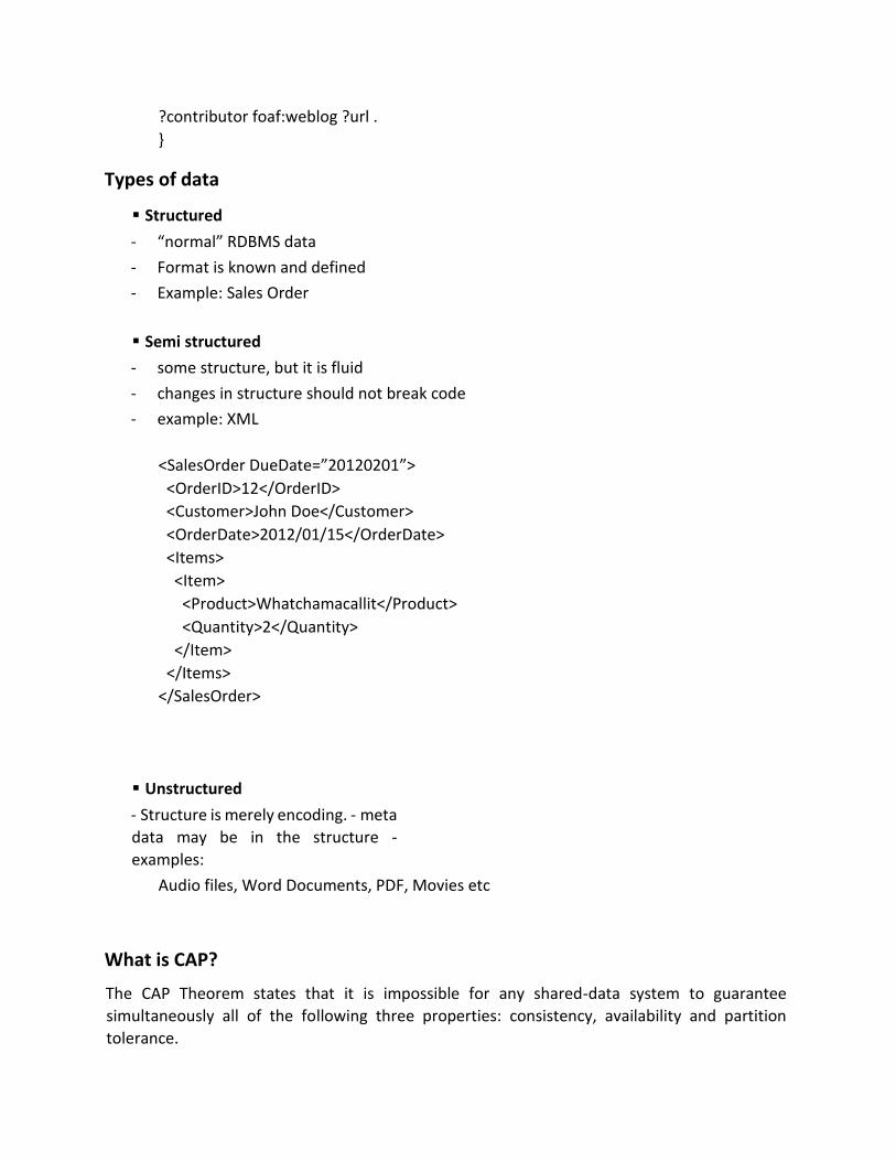
Types of data

Structured

- “normal” RDBMS data

- Format is known and defined

- Example: Sales Order

Semi structured

- some structure, but it is fluid

- changes in structure should not break code

- example: XML

<SalesOrder DueDate=”20120201”>

<OrderID>12</OrderID>

<Customer>John Doe</Customer>

<OrderDate>2012/01/15</OrderDate>

<Items>

<Item>

<Product>Whatchamacallit</Product>

<Quantity>2</Quantity>

</Item>

</Items>

</SalesOrder>

Unstructured

- Structure is merely encoding. - meta

data may be in the structure -

examples:

Audio files, Word Documents, PDF, Movies etc

What is CAP?

The CAP Theorem states that it is impossible for any shared-data system to guarantee

simultaneously all of the following three properties: consistency, availability and partition

tolerance.

Consistency in CAP is not the same as consistency in ACID (that would be too easy).

According to CAP, consistency in a database means that whenever data is written, everyone

who reads from the database will always see the latest version of the data. A database

without strong consistency means that when the data is written, not everyone who reads

from the database will see the new data right away; this is usually called eventual-

consistency or weak consistency.

Availability in a database according to CAP means you always can expect the database to be

there and respond whenever you query it for information. High availability usually is

accomplished through large numbers of physical servers acting as a single database

through sharing (splitting the data between various database nodes) and

replication (storing multiple copies of each piece of data on different nodes).

Partition tolerance in a database means that the database still can be read from and written to

when parts of it are completely inaccessible. Situations that would cause this include things like

when the network link between a significant numbers of database nodes is interrupted.

Partition tolerance can be achieved through some sort of mechanism whereby writes destined

for unreachable nodes are sent to nodes that are still accessible. Then, when the failed nodes

come back, they receive the writes they missed

Taxonomy of NOSQL implementation

The current NoSQL world fits into 4 basic categories.

Key-values Stores The Key-Value database is a very simple structure based on Amazon’s Dynamo DB. Data

is indexed and queried based on it’s key. Key-value stores provide consistent hashing so

they can scale incrementally as your data scales. They communicate node structure

through a gossip-based membership protocol to keep all the nodes synchronized. If you

are looking to scale very large sets of low complexity data, key-value stores are the best

option.

Examples: Riak, Voldemort etc

Column Family Stores were created to store and process very large amounts

of data distributed over many machines. There are still keys but they point

to multiple columns. In the case of BigTable (Google's Column Family NoSQL

model), rows are identified by a row key with the data sorted and stored by

this key. The columns are arranged by column family. E.g. Cassandra, HBase

etc

- These data stores are based on Google’s BigTable implementation. They may look similar

to relational databases on the surface but under the hood a lot has changed. A column

family database can have different columns on each row so is not relational and doesn’t

have what qualifies in an RDBMS as a table. The only key concepts in a column family

database are columns, column families and super columns. All you really need to start

with is a column family. Column families define how the data is structured on disk. A

column by itself is just a key-value pair that exists in a column family. A super column is

like a catalogue or a collection of other columns except for other super columns.

- Column family databases are still extremely scalable but less-so than key value stores.

However, they work better with more complex data sets.

Document Databases were inspired by Lotus Notes and are similar to

keyvalue stores. The model is basically versioned documents that are

collections of other key-value collections. The semi-structured documents

are stored in formats like JSON e.g. MongoDB, CouchDB

- A document database is not a new idea. It was used to power one of the

more prominent communication platforms of the 90’s and still in service

today, Lotus Notes now called Lotus Domino. APIs for document DBs use

Restful web services and JSON for message structure making them easy to

move data in and out.

- A document database has a fairly simple data model based on collections of

key-value pairs.

- A typical record in a document database would look like this:

- { “Subject”: “I like Plankton”

“Author”: “Rusty”

“PostedDate”: “5/23/2006″

“Tags”: ["plankton", "baseball", "decisions"]

“Body”: “I decided today that I don’t like baseball. I like plankton.” }

- Document databases improve on handling more complex structures but are

slightly less scalable than column family databases.

Graph Databases are built with nodes, relationships between notes and the

properties of nodes. Instead of tables of rows and columns and the rigid

structure of SQL, a flexible graph model is used which can scale across many

machines.

- Graph databases take document databases to the extreme by introducing

the concept of type relationships between documents or nodes. The most

common example is the relationship between people on a social network

such as Facebook. The idea is inspired by the graph theory work by Leonhard

Euler, the 18th century mathematician. Key/Value stores used key-value

pairs as their modeling units. Column Family databases use the tuple with

attributes to model the data store. A graph database is a big dense network

structure.

- While it could take an RDBMS hours to sift through a huge linked list of

people, a graph database uses sophisticated shortest path algorithms to

make data queries more efficient. Although slower than its other NoSQL

counterparts, a graph database can have the most complex structure of

them all and still traverse billions of nodes and relationships with light speed.

Cassandra

Cassandra is now deployed as the backend storage system for multiple services within

Facebook

To meet the reliability and scalability needs described above Facebook has developed

Cassandra.

Cassandra was designed to full the storage needs of the Search problem.

Data Model

Cassandra is a distributed key-value store.

A table in Cassandra is a distributed multi-dimensional map indexed by a key. The value

is an object which is highly structured.

The row key in a table is a string with no size restrictions, although typically 16 to 36

bytes long.

Every operation under a single row key is atomic per replica no matter how many

columns are being read or written into.

Columns are grouped together into sets called column families.

Cassandra exposes two kinds of columns families, Simple and Super column families.

Super column families can be visualized as a column family within a column family.

Architecture

Cassandra is designed to handle big data workloads across multiple nodes with no single

point of failure.

Its architecture is based in the understanding that system and hardware failure can and

do occur.

Cassandra addresses the problem of failures by employing a peer-to-peer distributed

system where all nodes are the same and data is distributed among all nodes in the

cluster.

Each node exchanges information across the cluster every second.

A commit log on each node captures write activity to ensure data durability.

Data is also written to an in-memory structure, called a memtable, and then written to

a data file called an SStable on disk once the memory structure is full.

All writes are automatically partitioned and replicated throughout the cluster.

Client read or write requests can go to any node in the cluster.

When a client connects to a node with a request, that node serves as the coordinator for

that particular client operation.

The coordinator acts as a proxy between the client application and the nodes that own

the data being requested.

The coordinator determines which nodes in the ring should get the request based on

how the cluster is configured.

Mongo DB

MongoDB is an open source, document-oriented database designed with both scalability and

developer agility in mind.

Instead of storing data in tables and rows like as relational database, in MongoDB store JSONlike

documents with dynamic schemas (schema-free, schema less).

Master/slave replication (auto failover with replica sets)

Sharding built-in

Queries are javascript expressions

Run arbitrary javascript functions server-side

Better update-in-place than CouchDB

Uses memory mapped files for data storage

An empty database takes up 192Mb

GridFS to store big data + metadata (not actually an FS)

Data model

Data model: Using BSON (binary JSON), developers can easily map to modern

objectoriented languages without a complicated ORM layer.

BSON is a binary format in which zero or more key/value pairs are stored as a single

entity.

Lightweight, traversable, efficient.

Schema design

{

"_id" : ObjectId("5114e0bd42…"),

"first" : "John",

"last" : "Doe",

"age" : 39,

"interests" : [

"Reading",

"Mountain Biking ]

"favorites": {

"color": "Blue",

"sport": "Soccer"}

}

Architecture

1. Replication

Replica Sets and Master-Slave

Replica sets are a functional superset of master/slave.

Architecture (Write process)

All write operation go through primary, which applies the write operation.

write operation than records the operations on primary’s operation log “oplog”

Secondary are continuously replicating the oplog and applying the operations to

themselves in a asyn0chronous process.

Why replica sets?

Data Redundancy

Automated Failover

Read Scaling

Maintenance

Disaster Recovery(delayed secondary)

2. Sharding

Sharding is the partitioning of data among multiple machines in an order-preserving

manner.(horizontal scaling )

Hbase

HBase was created in 2007 at Powerset and was initially part of the contributions in

Hadoop.

Since then, it has become its own top-level project under the Apache Software

Foundation umbrella.

It is available under the Apache Software License, version 2.0.

Features

non-relational

distributed

Opensource

and horizontal scalable.

Multi-dimensional rather than 2-D (relational)

schema-free

Decentralized Storage System easy replication support simple API, etc.

Architecture

Tables, Rows, Columns, and Cells

the most basic unit is a column.

One or more columns form a row that is addressed uniquely by a row key.

A number of rows, in turn, form a table, and there can be many of them. Each column

may have distinct value contained in a separate cell.

All rows are always sorted lexicographically by their row key.

Rows are composed of columns, and those, in turn, are grouped into column families. All

columns in a column family are stored together in the same low level storage file, called an HFile.

Millions of columns in a particular column family. There is also no type nor length boundary on

the column values.

Rows and columns in HBase

Google Bigtable

A Bigtable is a sparse, distributed, persistent multidimensional sorted map. The map is indexed by a row

key, column key, and a timestamp; each value in the map is an uninterpreted array of bytes.

Google's BigTable and other similar projects (ex: CouchDB, HBase) are database systems that are

oriented so that data is mostly denormalized (ie, duplicated and grouped).

The main advantages are: - Join operations are less costly because of the denormalization -

Replication/distribution of data is less costly because of data independence (ie, if you want to distribute

data across two nodes, you probably won't have the problem of having an entity in one node and other

related entity in another node because similar data is grouped)

This kind of systems are indicated for applications that need to achieve optimal scale (ie, you add more

nodes to the system and performance increases proportionally). In an ORM like MySQL or Oracle, when

you start adding more nodes if you join two tables that are not in the same node, the join cost is higher.

This becomes important when you are dealing with high volumes.

ORMs are nice because of the richness of the storage model (tables, joins). Distributed databases are nice

because of the ease of scale.

Questions

Explain NoSQL with its features.

A NoSQL database provides a mechanism for storage and retrieval of data that uses looser

consistency models than traditional relational databases. Motivations for this approach include

simplicity of design, horizontal scaling and finer control over availability. NoSQL databases are

often highly optimized key–value stores intended for simple retrieval and appending operations,

with the goal being significant performance benefits in terms of latency and throughput. NoSQL

databases are finding significant and growing industry use in big data and real-time web

applications. NoSQL systems are also referred to as "Not only SQL" to emphasize that they do in

fact allow SQL-like query languages to be used. Unlike RDBMS, NoSQL cannot necessarily give

full ACID guarantees, and are characterized by BASE, which means Basically Available, Soft state

and Eventually Consistent. Moreover, there are many types of NOSQL in its literature. The types

are basically guided by CAP theorem. CAP stands for Consistency, Availability and Partitioning.

The theorem states, that for NoSQL, we have to sacrifice one of the three, and cannot

simultaneously achieve all. Most of NoSQL databases sacrifices consistency, while in RDBMS,

partitioning is sacrificed and other 2 are always achieved.

Features of NoSQL:

Ability to horizontally scale the simple operations throughput over many servers

Ability to replicate and partition data over many servers

A simpler API, and no query language

Weaker concurrency model than ACID transactions

Efficient use of distributed indexes and RAM for storage

Ability to dynamically add new attributes to data records

Why does normalization fail in data analytics scenario?

Data analytics is always associated with big data, and when we say Big Data, we always have to

remember the “three V’s” of big data, i.e. volume, velocity and variety. NoSQL databases are

designed keeping these three V’s in mind. But RDBMS are strict, i.e. they have to follow some

predefined schema. Schema are designed by normalization of various attributes of data. The

downside of many relational data warehousing approaches is that they're rigid and hard to

change. You start by modeling the data and creating a schema, but this assumes you know all

the questions you'll need to answer. When new data sources and new questions arise, the

schema and related ETL and BI applications have to be updated, which usually requires an

expensive, time-consuming effort. But, this is not problem for big data scenario. They are made

to handle the “variety” of data. There is no schema in NoSQL. Attributes can be dynamically

added. Normalization is done so that duplicates can be minimized as far as possible, but NoSQL

and Big Data do not care about duplicates and storage. This is because, unlike RDBMS, NoSQL

database storages are distributed over multiple clusters, and storage is never going to be

obsolete. We can easily configure and add new cluster if performance and storage demands.

This facility provided by distributed system APIs such as Hadoop is popularly known as horizontal

scaling. But in RBDMS, most of them are single node storage, the multimode parallel databases

are also available, but they are limited too, to just few nods and moreover costs much high. Due

to these reasons, normalization approach often fails for data analytics scenario.

Explain different HBase API's in short.

HBase is an open source, non-relational, distributed database modeled after Google's BigTable

and is written in Java. It is developed as part of Apache Software Foundation's Apache Hadoop

project and runs on top of HDFS (Hadoop Distributed Filesystem), providing BigTable-like

capabilities for Hadoop. That is, it provides a fault-tolerant way of storing large quantities of

sparse data. HBase features compression, in-memory operation, and Bloom filters on a

percolumn basis as outlined in the original Big Table paper. Tables in HBase can serve as the

input and output for MapReduce jobs run in Hadoop, and may be accessed through the Java API

but also through REST, Avro or Thrift gateway APIs HBase provide following commands in HBase

shell:

General Commands:

- status : Shows server status

- version : Shows version of HBase

2. DDL Commands:

- alter : Using this command you can alter the table

- create : create table in hbase - describe : Gives table Description -

disable : Start disable of named table:

- drop : Drop the named table.

- enable : Start enable of named table

- exists : Does the named table exist? e.g. "hbase> exists 't1'"

- is_disabled : Check if table is disabled

- is_enabled : Check if table is enabled

- list : List out all the tables present in hbase

DML Commands:

- count :Count the number of rows in a table.

- Delete Put a delete cell value at specified table/row/column and optionally

timestamp coordinates. Deletes must match the deleted cell's coordinates

exactly.

- Deleteall Delete all cells in a given row; pass a table name, row, and optionally a

column and timestamp

- Get Get row or cell contents; pass table name, row, and optionally a dictionary of

column(s), timestamp, timerange and versions.

- get_counter Return a counter cell value at specified table/row/column

coordinates. A cell should be managed with atomic increment function oh HBase

and the data should be binary encoded.

- Incr Increments a cell 'value' at specified table/row/column coordinates.

- Put Put a cell 'value' at specified table/row/column and optionally timestamp

coordinates.

- Scan Scan a table; pass table name and optionally a dictionary of scanner

specifications. Scanner specifications may include one or more of: TIMERANGE,

FILTER, LIMIT, STARTROW, STOPROW, TIMESTAMP, MAXLENGTH, or COLUMNS.

If no columns are specified, all columns will be scanned.

- Truncate Scan a table; pass table name and optionally a dictionary of scanner

specifications. Scanner specifications may include one or more of: TIMERANGE,

FILTER, LIMIT, STARTROW, STOPROW, TIMESTAMP, MAXLENGTH, or COLUMNS.

If no columns are specified, all columns will be scanned.

Explain CAP theorem’s implications on Distributed Databases like NoSQL.

The CAP theorem was formally proved to be true by Seth Gilbert and Nancy Lynch of MIT in

2002. In distributed databases like NoSQL, however, it is very likely that we will have network

partitioning, and that at some point, machines will fail and cause others to become unreachable.

Packet loss, too, is nearly inevitable. This leads us to the conclusion that a distributed database

system must do its best to continue operating in the face of network partitions (to be

PartitionTolerant), leaving us with only two real options to choose from: Availability and

Consistency. Figure below illustrates visually that there is no overlapping segment where all

three are obtainable, thus explaining the concept of CAP theorem:

Suppose you are expected to design a Big Data application requiring to store data in some

NoSQL format. Which database would you use and what would govern your decision regarding

that?

Rational databases were never designed to cope with the scale and agility challenges that face

modern applications – and aren’t built to take advantage of cheap storage and processing power

that’s available today through the cloud. Database volumes have grown continuously since the

earliest days of computing, but that growth has intensified dramatically over the past decade as

databases have been tasked with accepting data feeds from customers, the public, point of sale

devices, GPS, mobile devices, RFID readers and so on. The demands of big data and elastic

provisioning call for a database that can be distributed on large numbers of hosts spread out

across a widely dispersed network. This give rise to the need of NoSQL database.

There exists wide variety of NoSQL database today. The choice of which database to be used in

the application depends greatly on the type of application being built. There are three primary

concern you must balance when choosing a data management system: consistency, availability,

and partition tolerance.

Consistency means that each client always has the same view of the data

Availability means that all clients can always read and write.

Partition tolerance means that the system works will across physical

network partitions.

According to the CAP Theorem, both Consistency and high Availability cannot be maintained

when a database is partitioned across a fallible wide area network. Now the choice of database

depends on the requirements trade-off between consistency and availability.

1. Consistent, Partition-Tolerant (CP) Systems have trouble with availability while keeping

data consistent across partitioned nodes. Examples of CP system include: Big Table,

Hypertable, HBase, MongoDB, Terrastore, Redis etc.

2. Available, Partitioned-Tolerant (AP) Systems achieve “eventual consistency” through

replication and verification. Example of AP systems include: Dynamo, Voldemort, Tokyo

Cabinet, Cassandra, CouchDB, SimpleDB, etc.

In addition to CAP configurations, another significant way data management systems vary is by

the data model they use: key-value, column-oriented, or document-oriented.

Key-value systems basically support get, put, and delete operations based on a primary

key. Examples: Tokyo Cabinet, Voldemort. Strengths: Fast lookups. Weaknesses: Stored

data has no schema.

Column-oriented systems still use tables but have no joins (joins must be handled within

your application). Obviously, they store data by column as opposed to traditional

roworiented databases. This makes aggregation much easier. Examples: Cassandra,

HBase. Strengths: Fast lookups, good distributed storage of data. Weaknesses: Very low-

level API.

Document-oriented systems store structured “documents” such as JSON or XML but have

no joins (joins must be handled within your application). It’s very easy to map data from

object-oriented software to these systems. Examples: CouchDB, MongoDb. Strengths:

Tolerant of incomplete data. Weaknesses: Query performance, no standard query

syntax.

Explain Eventual consistency and explain the reason why some NoSQL databases like

Cassandra sacrifice absolute consistency for absolute availability.

Eventual Consistency

Eventual consistency is a consistency model used in distributed computing that informally

guarantees that, if no new updates are made to given data then, eventually all accesses to that

item will return the last updated value. Eventual consistency is widely deployed in distributed

systems and has origins in early mobile computing projects. A system that has achieved eventual

consistency is often said to have converged, or achieved replica convergence. The reason why

so many NoSQL systems have eventual consistency is that virtually all of them are designed to

be distributed, and with fully distributed systems there is super-linear overhead to maintaining

strict consistency (meaning you can only scale so far before things start to slow down, and when

they do you need to throw exponentially more hardware at the problem to keep scaling).

Analogy example of eventual consistency:

1. I tell you it’s going to rain tomorrow.

2. Your neighbor tells his wife that it’s going to be sunny tomorrow.

3. You tell your neighbor that it is going to rain tomorrow.

Eventually, all of the servers (you, me, your neighbor) know the truth (that it’s going to rain

tomorrow) but in the meantime the client (his wife) came away thinking it is going to be sunny,

even though she asked after one of the servers knew the truth.

Absolute availability versus absolute consistency

Again from the CAP theorem, we cannot have the system which has both strict consistency and

strict availability provided the system is partitioning tolerant. Availability of the system has

higher priority to consistency in most cases. There are plenty of data models which are amenable

to conflict resolution and for which stale reads are acceptable ironically (many of these data

models are in the financial industry) and for which unavailability results in massive bottom-line

loses. If a system chooses to provide Consistency over Availability in the presence of partitions,

it will preserve the guarantees of its atomic reads and writes by refusing to respond to some

requests. It may decide to shut down entirely (like the clients of a single-node data store), refuse

writes (like Two-Phase Commit). But this condition is not tolerable in most of the system. Perfect

example is Facebook. Facebook needs 100% server uptime to serve its user all the time. If it

follows strict consistency sacrificing the strict availability, sometime it may refuse the client

request, need to shut down the node entirely showing users the unavailable message. And the

result is obvious, it loses its users every day leading to massive loss. The researcher has found

many ways by which one can gain the relaxed consistency (eventual consistency). Some of them

are (taking example of Cassandra):

Hinted Handoff

The client performs a write by sending the request to any Cassandra node which will act as the

proxy to the client. This proxy node will located N corresponding nodes that holds the data

replicas and forward the write request to all of them. In case any node is failed, it will pick a

random node as a handoff node and write the request with a hint telling it to forward the write

back to the failed node after it recovers. The handoff node will then periodically check for the

recovery of the failed node and forward the write to it. Therefore, the original node will

eventually receive all the write request.

Read Repair

When the client performs a “read”, the proxy node will issue N reads but only wait for R copies

of responses and return the node with the latest version. In case some nodes respond with an

older version, the proxy node will send the latest version to them asynchronously, hence these

left-behind node will still eventually catch up with the latest version.

Anti-Entropy data sync

To ensure the data is still sync even there is no READ and WRITE occurs to the data, replica nodes

periodically gossip with each other to figure out if anyone out of sync. For each key range of

data, each member in the replica group compute a Merkel tree (a hash encoding tree where the

difference can be located quickly) and send it to other neighbors. By comparing the received

Markel tree with its own tree, each member can quickly determine which data portion is out of

sync. If so, it will send diff to the left-behind members.

Why does traditional relational databases cannot provide partitioning of data using distributed

systems?

Several technical challenges make this quite difficult to do in practice. Apart from the added

complexity of building a distributed system the architect of a distributed DBMS has to overcome

some tricky engineering problems.

Atomicity on distributed system:

If the data updated by a transaction is spared across multiple nodes the commit/callback of the

nodes must be coordinated. This adds a significant overhead on shared-nothing systems. On

shared-disk systems this is less of an issue as all of the storage can be seen by all of the nodes so

a single node can coordinate the commit.

Consistency on distributed systems:

To take the foreign key, the system must be able to evaluate a consistent state. For example, if

the parent and child of a foreign key relationship could reside on different nodes some sort of

distributed locking mechanism is needed to ensure that outdated information is not used to

validate the transaction. If this is not enforced you could have (for example) a race condition

where the parent is deleted after its presence is verified before allowing the insert of the child.

Delayed enforcement of constraints (i.e. waiting until commit to validate DRI) requires the lock

to be held for the duration of the transaction. This sort of distributed locking comes with a

significant overhead. If multiple copies of data are held (this may be necessary on shared-

nothing systems to avoid unnecessary network traffic from semi-joins) then all copies of the data

must be updated.

Isolation on distributed system: Where data affected on a transaction resides on multiple system

nodes the locks and version (if MVCC is in use) must be synchronized across the nodes.

Guaranteeing serialisability of operations, particularly on shared-nothing architectures where

redundant copies of data may be stored requires a distributed synchronization mechanism such

as Lamport's Algorithm, which also comes with a significant overhead in network traffic.

Durability on distributed systems: On a shared disk system the durability issue is essentially the

same as a shared-memory system, with the exception that distributed synchronization protocols

are still required across nodes. The DBMS must journal writes to the log and write the data out

consistently. On a shared-nothing system there may be multiple copies of the data or parts of

the data stored on different nodes. A two-phase commit protocol is needed to ensure that the

commit happens correctly across the nodes. This also incurs significant overhead. On a

sharednothing system the loss of a node can mean data is not available to the system. To

mitigate this data may be replicated across more than one node. Consistency in this situation

means that the data must be replicated to all nodes where it normally resides. This can incur

substantial overhead on writes. One common optimization made in NoSQL systems is the use of

quorum replication and eventual consistency to allow the data to be replicated lazily while

guaranteeing a certain level of resiliency of the data by writing to a quorum before reporting the

transaction as committed. The data is then replicated lazily to the other nodes where copies of

the data reside. Note that 'eventual consistency' is a major trade-off on consistency that may

not be acceptable if the data must be viewed consistently as soon as the transaction is

committed. For example, on a financial application an updated balance should be available

immediately.

Chapter 5: Searching and Indexing

Indexing

Indexing is the initial part of all search applications.

Its goal is to process the original data into a highly efficient cross-reference lookup in

order to facilitate rapid searching.

The job is simple when the content is already textual in nature and its location is known.

Steps

acquiring the content.

This process gathers and scopes the content that needs to be indexed.

build documents

The raw content that needs to be indexed has to be translated into the units (usually

called documents) used by the search application.

document analysis

The textual fields in a document cannot be indexed directly. Rather, the text has to be

broken into a series of individual atomic elements called tokens.

This happens during the document analysis step. Each token corresponds roughly to a

word in the language, and the analyzer determines how the textual fields in the

document are divided into a series of tokens.

index the document

The final step is to index the document. During the indexing step, the document is added

to the index.

Lucene

Lucene is a free, open source project implemented in Java.

licensed under Apache Software Foundation.

Lucene itself is a single JAR (Java Archive) file, less than 1 MB in size, and with no

dependencies, and integrates into the simplest Java stand-alone console program as well

as the most sophisticated enterprise application.

Rich and powerful full-text search library.

Lucene to provide full-text indexing across both database objects and documents in

various formats (Microsoft Office documents, PDF, HTML, text, and so on).

supporting full-text search using Lucene requires two steps:

creating a lucence index

creating a lucence index on the documents and/or database objects.

Parsing looking up parsing the user query and looking up the prebuilt index to answer

the query.

Architecture

Creating an index (IndexWriter Class)

The first step in implementing full-text searching with Lucene is to build an index.

To create an index, the first thing that need to do is to create an IndexWriter object.

The IndexWriter object is used to create the index and to add new index entries (i.e.,

Documents) to this index. You can create an IndexWriter as follows

IndexWriter indexWriter = new IndexWriter("index-directory", new StandardAnalyzer(),

true);

Parsing the Documents (Analyzer Class)

The job of Analyzer is to "parse" each field of your data into indexable "tokens" or

keywords.

Several types of analyzers are provided out of the box. Table 1 shows some of the more

interesting ones.

StandardAnalyzer

A sophisticated general-purpose analyzer.

WhitespaceAnalyzer

A very simple analyzer that just separates tokens using white space.

StopAnalyzer

Removes common English words that are not usually useful for indexing.

SnowballAnalyzer

An interesting experimental analyzer that works on word roots (a search on rain should

also return entries with raining, rained, and so on).

Adding a Document/object to Index (Document Class)

.To index an object, we use the Lucene Document class, to which we add the fields that

you want indexed.

Document doc = new Document();

doc.add(new Field("description", hotel.getDescription(), Field.Store.YES,

Field.Index.TOKENIZED));

Elastic search

Elasticsearch is a search server based on Lucene. It provides a distributed, multitenant-capable

full-text search engine with aRESTful web interface and schema-free JSON documents.

Elasticsearch is developed in Java and is released as open source under the terms of the Apache

License.

Questions

Describe different components of enterprise search application from the raw content to index

creation and then querying the index.

An enterprise search application starts with an indexing chain, which in turn requires separate

steps to retrieve the raw content; create documents from the content, possibly extracting text

from binary documents; and index the documents. Once the index is built, the components

required for searching are equally diverse, including a user interface, a means for building up a

programmatic query, query execution (to retrieve matching documents), and results rendering.

The following figure illustrates the typical components of a search application:

Components for Index Creation

To search large amounts of raw content quickly, we must first index that content and convert it

into a format that will let us search it rapidly, eliminating the slow sequential scanning process.

This conversion process is called indexing, and its output is called an index. Thus, we can think

of an index as a data structure that allows fast random access to words stored inside it.

Acquire Content

The first step, at the bottom of figure, is to acquire content. This process, which involves

using a crawler or spider, gathers and scopes the content that needs to be indexed. That

may be trivial, for example, if we’re indexing a set of XML files that resides in a specific

directory in the file system or if all our content resides in a well-organized database.

Alternatively, it may be horribly complex and messy if the content is scattered in all sorts

of places. It needs to be incremental if the content set is large.

Build Document

Once we have the raw content that needs to be indexed, we must translate the content

into the units (usually called documents) used by the search engine. The document

typically consists of several separately named fields with values, such as title, body,

abstract, author, and URL. A common part of building the document is to inject boosts

to individual documents and fields that are deemed more or less important.

Analyze Document

No search engine indexes text directly: rather, the text must be broken into a series of

individual atomic elements called tokens. This is what happens during the Analyze

Document step. Each token corresponds roughly to a “word” in the language, and this

step determines how the textual fields in the document are divided into a series of

tokens.

Index Document

During the indexing step, the document is added to the index.

Components for Querying/Searching the Index

Querying or searching is the process of looking up words in an index to find documents where

they appear. The components for searching the index are as follows:

Search User Interface The user interface is what users actually see, in the web

browser, desktop application, or mobile device, when they interact with the

search application. The UI is the most important part of any search application.

Build Query when we manage to entice a user to use the search application, she

or he issues a search request, often as the result of an HTML form or Ajax request

submitted by a browser to the server. We must then translate the request into

the search engine’s Query object. This is called build query step. The user query

can be simple or complex.

Run Query/Search Query Search Query is the process of consulting the search

index and retrieving the documents matching the Query, sorted in the requested

sort order. This component covers the complex inner workings of the search

engine.

Render Results once we have the raw set of documents that match the query,

sorted in the right order, we then render them to the user in an intuitive,

consumable manner. The UI should also offer a clear path for follow-on searches

or actions, such as clicking to the next page, refining the search, or finding

documents similar to one of the matches, so that the user never hits a dead end.

Explain Elastic Search as a search engine technology

Elastic search is a tool for querying written words. It can perform some other nifty tasks, but at

its core it’s made for wading through text, returning text similar to a given query and/or

statistical analyses of a corpus of text. More specifically, elastic search is a standalone database

server, written in Java that takes data in and stores it in a sophisticated format optimized for

language based searches. Working with it is convenient as its main protocol is implemented with

HTTP/JSON. Elastic search is also easily scalable, supporting clustering out of the box, hence the

name elastic search. Whether it’s searching a database of retail products by description, finding

similar text in a body of crawled web pages, or searching through posts on a blog, elastic search

is a fantastic choice. When facing the task of cutting through the semi-structured muck that is

natural language, Elastic search is an excellent tool. What Problems does Elastic search solve

well? There are myriad cases in which elastic search is useful. Some use cases more clearly call

for it than others. Listed below are some tasks which for which elastic search is particularly well

suited.

Searching a large number of product descriptions for the best match for a specific

phrase (say “chef’s knife”) and returning the best results

Given the previous example, breaking down the various departments where

“chef’s knife” appears (see Faceting later in this book)

Searching text for words that sound like “season”

Auto-completing a search box based on partially typed words based on previously

issued searches while accounting for misspellings

Storing a large quantity of semi-structured (JSON) data in a distributed fashion,

with a specified level of redundancy across a cluster of machines.

It should be noted, however, that while elastic search is great at solving the aforementioned

problems, it’s not the best choice for others. It’s especially bad at solving problems for which

relational databases are optimized. Problems such as those listed below.

Calculating how many items are left in the inventory

Figuring out the sum of all line-items on all the invoices sent out in a given month

Executing two operations transnationally with rollback support

Creating records that are guaranteed to be unique across multiple given terms,

for instance a phone number and extension

Elastic search is generally fantastic at providing approximate answers from data, such as scoring

the results by quality. While elastic search can perform exact matching and statistical

calculations, its primary task of search is an inherently approximate task. Finding approximate

answers is a property that separates elastic search from more traditional databases. That being

said, traditional relational databases excel at precision and data integrity, for which elastic

search and Lucene have few provisions.

How would you use Elastic Search for implementing search engine in your project requiring

search facility?

Elastic Search is a distributed, RESTful, free/open source search server based on Apache Lucene.

It is developed by Shay Banon and is released under the terms of the Apache License. Elastic

Search is developed in Java. Apache Lucene is a high performance, full-featured Information

Retrieval library, written in Java. Elastic search uses Lucene internally to build its state of the art

distributed search and analytics capabilities. Now, we’ve a scenario to implement the search

feature to an application. We’ve tackled getting the data indexed, but now it’s time to expose

the full-text searching to the end users. It’s hard to imagine that adding search could be any

simpler than it is with Lucene. Obtaining search results requires only a few lines of code—

literally. Lucene provides easy and highly efficient access to those search results, too, freeing

you to focus on your application logic and UI around those results. When we search with Lucene,

we’ll have a choice of either programmatically constructing our query or using Lucene’s

QueryParser to translate text entered by the user into the equivalent Query. The first approach

gives us ultimate power, in that our application can expose whatever UI it wants, and our logic

translates interactions from that UI into a Query. But the second approach is wonderfully easy

to use, and offers a standard search syntax that all users are familiar with. As an example, let’s

take the simplest search of all: searching for all documents that contain a single term.

Example: Searching for a specific term

IndexSearcher is the central class used to search for documents in an index. It has several

overloaded search methods. You can search for a specific term using the most commonly used

search method. A term is a String value that’s paired with its containing field name—in our

example, subject. Lucene provides several built-in Querytypes, TermQuerybeing the most basic.

Lucene’s search methods require a Query object. Parsing a query expression is the act of

turning a user-entered textual query such as “mock OR junit” into an appropriate Query object

instance; in this case, the Query object would be an instance of Boolean-Query with two

optional clauses, one for each term.

Describe different type of analyzers available and its role in search engine development.

The index analysis module acts as a configurable registry of Analyzers that can be used in order

to both break indexed (analyzed) fields when a document is indexed and process query strings.

It maps to the Lucene Analyzer. Analyzers are (generally) composed of a single Tokenizer and

zero or more TokenFilters. A set of CharFilters can be associated with an analyzer to process the

characters prior to other analysis steps. The analysis module allows one to register TokenFilters,

Tokenizers and Analyzers under logical names that can then be referenced either in mapping

definitions or in certain APIs. The Analysis module automatically registers (if not explicitly

defined) built in analyzers, token filters, and tokenizers.

Types of Analyzers Analyzers in general are broken down into a Tokenizer with zero or more

TokenFilter applied to it. The analysis module allows one to register TokenFilters, Tokenizers and

Analyzers under logical names which can then be referenced either in mapping definitions or in

certain APIs. Here is a list of analyzer types: char filter

Char filters allow one to filter out the stream of text before it gets tokenized (used within an

Analyzer).

Tokenizer

Tokenizers act as the first stage of the analysis process (used within an Analyzer).

token filter

Token filters act as additional stages of the analysis process (used within an Analyzer).

default analyzers

An analyzer is registered under a logical name. It can then be referenced from mapping

definitions or certain APIs. When none are defined, defaults are used. There is an option to

define which analyzers will be used by default when none can be derived.

The default logical name allows one to configure an analyzer that will be used both for indexing

and for searching APIs. The default index logical name can be used to configure a default

analyzer that will be used just when indexing, and the default search can be used to configure a

default analyzer that will be used just when searching.

In Lucene, analyzers can also be classified as:

WhitespaceAnalyzer, as the name implies, splits text into tokens on whitespace characters and

makes no other effort to normalize the tokens. It doesn’t lower-case each token.

SimpleAnalyzer first splits tokens at non-letter characters, then lowercases each token. Be

careful! This analyzer quietly discards numeric characters but keeps all other characters.

StopAnalyzer is the same as SimpleAnalyzer, except it removes common words. By default, it

removes common words specific to the English language (the, a, etc.), though you can pass in

your own set.

StandardAnalyzer is Lucene’s most sophisticated core analyzer. It has quite a bit of logic to

identify certain kinds of tokens, such as company names, email addresses, and hostnames. It

also lowercases each token and removes stop words and punctuation.

Chapter 6. Case Study: Hadoop

What is Hadoop?

Hadoop is an open source software project that enables the distributed processing of large data

sets across clusters of commodity servers. It is designed to scale up from a single server to

thousands of machines, with a very high degree of fault tolerance. Rather than relying on

highend hardware, the resiliency of these clusters comes from the software’s ability to detect

and handle failures at the application layer.

HDFS

Hadoop Distributed File System (HDFS) is a file system that spans all the nodes in a Hadoop

cluster for data storage. It links together the file systems on many local nodes to make them into

one big file system.

Hadoop enables a computing solution that is:

Scalable– New nodes can be added as needed, and added without needing to change

data formats, how data is loaded, how jobs are written, or the applications on top.

Cost effective– Hadoop brings massively parallel computing to commodity servers. The

result is a sizeable decrease in the cost per terabyte of storage, which in turn makes it

affordable to model all your data.

Flexible– Hadoop is schema-less, and can absorb any type of data, structured or not, from

any number of sources. Data from multiple sources can be joined and aggregated in

arbitrary ways enabling deeper analyses than any one system can provide.

Fault tolerant– When you lose a node, the system redirects work to another location of

the data and continues processing without missing a fright beat.

Hadoop Daemons

Hadoop consist of five daemons

NameNode

DataNode

Secondary nameNode

Job tracker

Task tracker

“Running Hadoop” means running a set of daemons, or resident programs, on the different

servers in your network. These daemons have specific roles; some exist only on one server, some

exist across multiple servers.

Name node

Hadoop employs a master/slave architecture for both distributed storage and distributed

computation.

The distributed storage system is called the Hadoop File System, or HDFS.

The NameNode is the master of HDFS that directs the slave DataNode daemons to

perform the low-level I/O tasks.

The NameNode is the bookkeeper of HDFS; it keeps track of how your files are broken down into

file blocks, which nodes store those blocks, and the overall health of the distributed file system.

The function of the NameNode is memory and I/O intensive. As such, the server hosting the

NameNode typically doesn’t store any user data or perform any computations for a MapReduce

program to lower the workload on the machine.

it’s a single point of failure of your Hadoop cluster.

For any of the other daemons, if their host nodes fail for software or hardware reasons, the

Hadoop cluster will likely continue to function smoothly or you can quickly restart it. Not so for

the NameNode.

DataNode

Each slave machine in cluster host a DataNode daemon to perform work of the

distributed file system, reading and writing HDFS blocks to actual files on the local file

system.

Read or write a HDFS file, the file is broken into blocks and the NameNode will tell your

client which DataNode each block resides in.

Job communicates directly with the DataNode daemons to process the local files

corresponding to the blocks.

Furthermore, a DataNode may communicate with other DataNodes to replicate its data

blocks for redundancy.

Secondary NameNode

Each slave machine in cluster host a DataNode daemon to perform work of the

distributed file system, reading and writing HDFS blocks to actual files on the local file

system.

Read or write a HDFS file, the file is broken into blocks and the NameNode will tell

your client which DataNode each block resides in.

Job communicates directly with the DataNode daemons to process the local files

corresponding to the blocks.

Furthermore, a DataNode may communicate with other DataNodes to replicate its

data blocks for redundancy.

JobTracker

The JobTracker daemon is the liaison (mediator) between your application and Hadoop.

Once you submit your code to your cluster, the JobTracker determines the execution

plan by determining which files to process, assigns nodes to different tasks, and monitors

all tasks as they’re running.

Should a task fail, the JobTracker will automatically re launch the task, possibly on a

different node, up to a predefined limit of retries.

There is only one JobTracker daemon per Hadoop cluster.

It’s typically run on a server as a master node of the cluster

Task tracker

The JobTracker daemon is the liaison (mediator) between your application and Hadoop.

Once you submit your code to your cluster, the JobTracker determines the execution

plan by determining which files to process, assigns nodes to different tasks, and monitors

all tasks as they’re running.

Should a task fail, the JobTracker will automatically re launch the task, possibly on a

different node, up to a predefined limit of retries.

There is only one JobTracker daemon per Hadoop cluster.

It’s typically run on a server as a master node of the cluster

Hadoop configuration modes

Local (standalone mode)

The standalone mode is the default mode for Hadoop.

Hadoop chooses to be conservative and assumes a minimal configuration. All XML

(Configuration) files are empty under this default mode.

With empty configuration files, Hadoop will run completely on the local machine.

Because there’s no need to communicate with other nodes, the standalone mode doesn’t

use HDFS, nor will it launch any of the Hadoop daemons.

Its primary use is for developing and debugging the application logic of a Map-Reduce

program without the additional complexity of interacting with the daemons.

Pseudo-distributed mode

The pseudo-distributed mode is running Hadoop in a “cluster of one” with all daemons

running on a single machine.

This mode complements the standalone mode for debugging your code, allowing you to

examine memory usage, HDFS input/output issues, and other daemon interactions.

Need Configuration on XML Files hadoop/conf/.

Fully distributed mode

Benefits of distributed storage and distributed computation

master—The master node of the cluster and host of the NameNode and Job-Tracker

daemons

backup—The server that hosts the Secondary NameNode daemon

hadoop1, hadoop2, hadoop3, ...—The slave boxes of the cluster running both DataNode

and TaskTracker daemons

Working with files in HDFS

HDFS is a file system designed for large-scale distributed data processing under

frameworks such as Map-Reduce.

Store a big data set of (say) 100 TB as a single file in HDFS.

Replicate the data for availability and distribute it over multiple machines to enable

parallel processing.

HDFS abstracts these details away and gives you the illusion that you’re dealing with only

a single file.

Hadoop Java libraries for handling HDFS files programmatically.

Assumptions and goals

Hardware failure

Hardware failure is the norm rather than the exception.

An HDFS instance may consist of hundreds or thousands of server machines, each storing

part of the file system’s data.

The fact that there are a huge number of components and that each component has a

non-trivial probability of failure means that some component of HDFS is always

nonfunctional.

Therefore, detection of faults and quick, automatic recovery from them is a core

architectural goal of HDFS.

Streaming data access

Applications that run on HDFS need streaming access to their data sets.

They are not general purpose applications that typically run on general purpose file

systems.

HDFS is designed more for batch processing rather than interactive use by users.

The emphasis is on high throughput of data access rather than low latency of data access.

Large data sets

Applications that run on HDFS need streaming access to their data sets.

They are not general purpose applications that typically run on general purpose file

systems.

HDFS is designed more for batch processing rather than interactive use by users.

The emphasis is on high throughput of data access rather than low latency of data access.

Simple coherency model

HDFS applications need a write-once-read-many access model for files.

A file once created, written, and closed need not be changed.

This assumption simplifies data coherency issues and enables high throughput data

access.

A Map/Reduce application or a web crawler application fits perfectly with this model.

There is a plan to support appending-writes to files in the future.