Big Data Network Traffic Summary Dataset - ONTIC · PDF file7.1.4 Samza ... Cisco OpenSOC...

Big Data Network Traffic Summary Dataset

Deliverable

ONTIC Big Data Architecture

ONTIC Project

(GA number 619633)

Deliverable D2.2 Dissemination Level: PUBLIC

Authors

Enrique Fernández, Alexandru Mara, Álex Martínez, Alberto Mozo,

Bruno Ordozgoiti, Stanislav Vakaruk, Bo Zhu. UPM

Fernando Arias, Vicente Martin.

EMC

Sotiria Chatzi, Evangelos Iliakis. ADAPTIT

Daniele Apiletti, Elena Baralis, Silvia Chiusano, Tania Cerquitelli, Paolo Garza, Luigi Grimaudo, Fabio Pulvirenti.

POLITO

Version

ONTIC_D2.2.2015.01.31.4

619633 ONTIC. Deliverable 2.2

2 / 48

Version History

Previous version Modification date

Modified by

Summary

2014.12.02.V.1 2014.12.24 ADAPTIT Compilation of individual partners

parts, first corrections.

2014.12.28.V.1.1 2015.01.15 UPM Added missing references,

acronyms and major

modifications to some sections.

2015.01.15.V.1.2 2015.01.16 ADAPTIT Review of modified / corrected version

2015.01.16.V.1 2015.01.20 UPM Changes to initial

sections, figures and references.

2015.01.20.2 2015.01.21 ADAPTIT Changes to figures, ANNEX

2015.01.21.2.1 2015.01.27 UPM Changes after revision

2015.01.31.4 2015.01.31 UPM Quality assurance

review

Quality Assurance:

Name

Quality Assurance Manager

Mozo Velasco, Alberto (UPM)

Reviewer #1 Miguel Angel, López (SATEC)

Reviewer #2 Apiletti, Daniele (POLITO)


3 / 48

Copyright © 2015, ONTIC Consortium

The ONTIC Consortium (http://www.http://ict-ontic.eu/) grants third parties the right to use and distribute all or parts of this document, provided that the ONTIC project and the document are

properly referenced.

THIS DOCUMENT IS PROVIDED BY THE COPYRIGHT HOLDERS AND CONTRIBUTORS "AS IS" AND ANY EXPRESS OR IMPLIED WARRANTIES, INCLUDING, BUT NOT LIMITED TO, THE IMPLIED WARRANTIES OF MERCHANTABILITY AND FITNESS FOR A PARTICULAR

PURPOSE ARE DISCLAIMED. IN NO EVENT SHALL THE COPYRIGHT OWNER OR CONTRIBUTORS BE LIABLE FOR ANY DIRECT, INDIRECT, INCIDENTAL, SPECIAL, EXEMPLARY, OR CONSEQUENTIAL DAMAGES (INCLUDING, BUT NOT LIMITED TO, PROCUREMENT OF SUBSTITUTE GOODS OR SERVICES; LOSS OF USE, DATA, OR

PROFITS; OR BUSINESS INTERRUPTION) HOWEVER CAUSED AND ON ANY THEORY OF LIABILITY, WHETHER IN CONTRACT, STRICT LIABILITY, OR TORT (INCLUDING

NEGLIGENCE OR OTHERWISE) ARISING IN ANY WAY OUT OF THE USE OF THIS DOCUMENT, EVEN IF ADVISED OF THE POSSIBILITY OF SUCH DAMAGE


4 / 48

Table of Contents

1. ACRONYMS AND DEFINITIONS 8

2. EXECUTIVE SUMMARY 10

3. SCOPE 11

4. INTENDED AUDIENCE 12

5. SUGGESTED PREVIOUS READINGS 13

6. INTRODUCTION TO BIG DATA ARCHITECTURE 14

6.1 Big Data Definition .............................................................................. 14

6.2 Map-Reduce paradigm and Hadoop ............................................................ 14

6.3 TM Forum Big Data Analytics Reference Architecture ...................................... 15

6.4 Big Data Pipeline ................................................................................ 16

7. RELATED ARCHITECTURES AND FRAMEWORKS 19

7.1 Distributed Computation frameworks ......................................................... 19

7.1.1 Hadoop .................................................................................................. 20 7.1.2 Spark .................................................................................................... 20 7.1.3 Storm .................................................................................................... 20 7.1.4 Samza ................................................................................................... 20 7.1.5 Flink ..................................................................................................... 21 7.1.6 SQL like query approaches for Big Data ............................................................ 21 7.1.7 Graph oriented solutions ............................................................................. 21

7.2 Online and Offline analytics frameworks ..................................................... 22

7.2.1 Weka ..................................................................................................... 22 7.2.2 MOA ...................................................................................................... 22 7.2.3 Mahout .................................................................................................. 22 7.2.4 MLlib ..................................................................................................... 22 7.2.5 Samoa ................................................................................................... 23 7.2.6 MADlib ................................................................................................... 23

7.3 Cisco OpenSOC Architecture ................................................................... 23

7.4 Platforms and frameworks benchmark ........................................................ 28

7.4.1 Objectives .............................................................................................. 28 7.4.2 Evaluation Metrics ..................................................................................... 28 7.4.3 Hardware and Software ............................................................................... 29 7.4.4 Description of the experiments ...................................................................... 29 7.4.5 Preliminary experiment ............................................................................... 30

8. ONTIC BIG DATA ARCHITECTURE 32


5 / 48

9. FEATURE ENGINEERING IN ONTIC 34

9.1 Introduction and requirements ................................................................ 34

9.2 Feature management ........................................................................... 36

9.3 Feature Selection ............................................................................... 40

9.3.1 CSSP Algorithms ........................................................................................ 41

9.4 Feature Reduction ............................................................................... 41

9.4.1 PCA ...................................................................................................... 42 9.4.2 PCA Experiments ....................................................................................... 43 9.4.3 Future experiments in plan .......................................................................... 44

ANNEX A - COPYRIGHT NOTICE AND DISCLAIMER- ANNEX 46

A.1 TM Forum copyright notice and disclaimer- Annex ........................................ 46

A.2 Open-source Projects copyright notice- Annex ............................................ 46

A.2.1 OpenSOC copyright notice – Annex ................................................................ 46

10. REFERENCES 47


6 / 48

List of figures Figure 1: Hadoop Framework ............................................................................... 14 Figure 2: TM Forum Big Data Analytics Reference Architecture ....................................... 15 Figure 3: Big Data Pipeline .................................................................................. 16 Figure 4: Big Data Batch (MR/YARN) or Micro-Batch (Spark) Pipeline ................................ 17 Figure 5: Big Data Streaming Pipeline ..................................................................... 17 Figure 6: Big Data Streaming Pipeline ..................................................................... 18 Figure 7: Cisco OpenSOC Logical Architecture ........................................................... 24 Figure 8: Cisco OpenSOC Deployment Infrastructure .................................................... 24 Figure 9: Cisco OpenSOC Component Architecture ...................................................... 25 Figure 10: Cisco OpenSOC PCAP Topology Structure .................................................... 26 Figure 11: Cisco OpenSOC DPI Topology Structure ....................................................... 27 Figure 12: Cisco OpenSOC PCAP Data Enrichment Topology Structure ............................... 27 Figure 13: Data storage and processing experiments.................................................... 30 Figure 14: Hadoop/Spark performance on different dataset sizes .................................... 31 Figure 15: ONTIC Big Data Architecture ................................................................... 32 Figure 16: ONTIC Feature Management Architecture. .................................................. 35 Figure 17: Feature Selection branch. ...................................................................... 40 Figure 18: Feature Selection branch. ...................................................................... 42 Figure 19: PCA of real network data with no expanded features. ..................................... 43 Figure 20: PCA of real data considering expanded features. ........................................... 44


7 / 48

List of tables Table 1: D2.2 Acronyms....................................................................................... 8 Table 2: Common features for BFS and FCBF. ............................................................ 38 Table 3: Features selected using NBK. .................................................................... 38 Table 4: Features selected using C4.5. .................................................................... 39 Table 5: Features selected using C4.5 on UNIBS dataset. .............................................. 39 Table 6: Features selected using C4.5 on CAIDA dataset. .............................................. 39


8 / 48

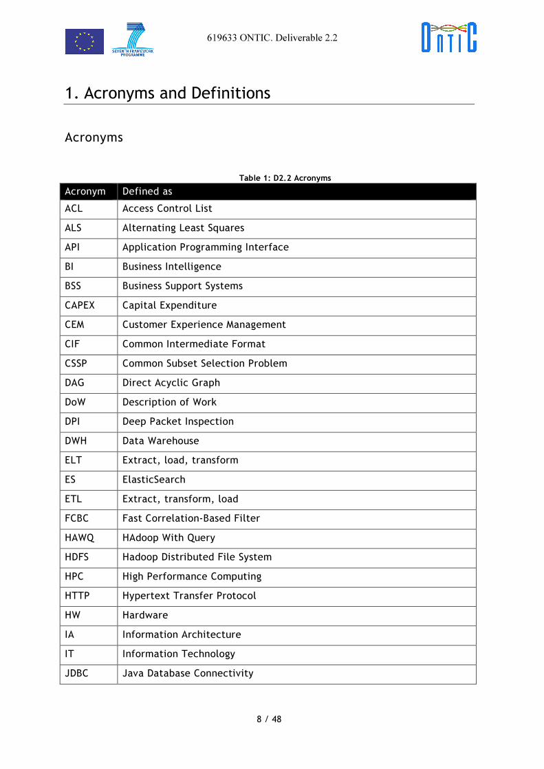
1. Acronyms and Definitions

Acronyms

Table 1: D2.2 Acronyms

Acronym Defined as

ACL Access Control List

ALS Alternating Least Squares

API Application Programming Interface

BI Business Intelligence

BSS Business Support Systems

CAPEX Capital Expenditure

CEM Customer Experience Management

CIF Common Intermediate Format

CSSP Common Subset Selection Problem

DAG Direct Acyclic Graph

DoW Description of Work

DPI Deep Packet Inspection

DWH Data Warehouse

ELT Extract, load, transform

ES ElasticSearch

ETL Extract, transform, load

FCBC Fast Correlation-Based Filter

HAWQ HAdoop With Query

HDFS Hadoop Distributed File System

HPC High Performance Computing

HTTP Hypertext Transfer Protocol

HW Hardware

IA Information Architecture

IT Information Technology

JDBC Java Database Connectivity


9 / 48

MCMC Monte Carlo Markov Chain

MOA Massive On-line Analysis

ML Machine Learning

MR Map-Reduce

NLANR National Laboratory for Applied Network Research

OpenSOC Open Security Operations Center

OPEX Operating Expense

ORC Optimized Row Columnar

OSS Operations Support Systems

PCA Principal Component Analysis

PCAP Packet Capture

RAM Random Access Memory

REST Representational state transfer

RPC Remote Procedure Call

RTT Round Trip Time

SPE Streaming Processing Engines

SQL Structured Query Language

SVD Singular Value Decomposition

SVM Support Vector Machines

SW Software

TCP Transmission Control Protocol

UDP User Datagram Protocol

WEKA Waikato Environment for Knowledge Analysis

YARN Yet Another Resource Negotiator


10 / 48

2. Executive Summary

The main target of this deliverable is the report of the initial requirements and the architectural design of the ONTIC Big Data Architecture. Additionally, this deliverable contains the procedures to create and deploy a big data platform as an instance of the ONTIC big data architecture.

An introduction to the big data architecture is being made to connect D2.2 to D2.1. Continuing, some related architectures are presented, in order to describe the state of the art. As a common storage and a processing big data strategy will be included in this architecture, Hadoop, Spark and Storm open source distributions will be part of the corner stones of this architecture. For this reason the three frameworks, are examined with some detail. Next, some other online and offline processing engines are presented and described.

To determine the basic components of the ONTIC Big Data Architecture, a comparison among the most used computation frameworks and libraries has been designed and is currently being performed. For this reason, results of tests and experiments performed so far are presented in this deliverable.

Then, the big data architecture is described, starting from the data capturing systems and moving on to the online and offline analytics platforms.

Since feature engineering is important for the attainment of efficient and effective big data analytics, a chapter of the deliverable has been devoted to Feature Engineering. More specifically, main feature selection and reduction techniques are explained. Finally, some preliminary experiment using the ONTIC dataset and Principal Components Analysis (PCA) as feature reduction technique are shown.


11 / 48

3. Scope

This document is part of WP2 of the ONTIC project which deals with designing, deploying, managing and provisioning with real ISP network packet traces a big data network Traffic Summary dataset (ONTS), as stated in the DoW of the project.

In deliverable D2.1: Requirements Strategy, the basis for the strategy and guidelines to be followed in this WP2 were stated. The main purpose for deliverable D2.2 is to make a first approach to the final big data architecture, evaluating different frameworks for big data processing that will be used along the project, based on the state of the art of this kind of technologies.

A second goal for this deliverable is to introduce the network feature selection management and lay down the requirements for the ONTS dataset. Concepts like feature selection and feature reduction are introduced, and will be refined along the project.

This document will be, as a consequence, the starting point for the deliverable D2.3: Progress on ONTIC Big Data Architecture, where the evolution of the requirements and the architecture of the ONTIC Big Data Architecture will be presented.


12 / 48

4. Intended audience

This document is specifically oriented to partners of the ONTIC project participating in work packages 2, 3 and 4 as the information provided here sets the basis on which they will be working during the rest of the project. This deliverable is also intended to any other reader interested in learning more about the Big Data Architecture proposed by ONTIC or distributed computation and analytics frameworks.


13 / 48

5. Suggested previous readings

This document makes reference to different standard and open source big data frameworks; as it is not the goal of this document to describe in detail the architecture of these platforms, we include here the main references where the reader can find all the information needed to understand them and so, to better comprehend the ONTIC Big Data Architecture proposed:

• Apache Hadoop project main page [1].

• Apache Spark project main page [1].

• Apache Storm project main page [2].

• Apache Samza project main page [3].

• Apache Flink project main page [4].

• HAWQ project main page [5].

• Cisco OpenSOC architecture description [6].


14 / 48

6. Introduction to Big Data Architecture

Big Data is nowadays a very common term in both research and industrial environments, but it still is, sometimes, used wrong. So in order to clarify the term and set the basis to understand the architecture designed and proposed here; this section will define what big data and big data architectures are and how these types of platforms work.

6.1 Big Data Definition The three Vs model, volume (amount of data), velocity (speed of data in and out), and variety (range of data types and sources), remains the dominating model to define the term big data. Therefore, big data is a term used to refer to systems able to cope with information that cannot be handled by traditional data processing systems because of its volume, velocity and/or variety.

6.2 Map-Reduce paradigm and Hadoop Currently, the most common approach for big data processing in the industrial sector is the Map-Reduce paradigm proposed by Google [8]. This paradigm is designed to efficiently process large volumes of data, by connecting many commodity computers (cluster) together, to work in parallel. Map-Reduce breaks the data flow into two phases, namely the map phase and the reduce phase. In map phase, chunks of data are processed in isolation and in parallel by tasks called mappers. The outputs of these mappers are brought into tasks called reducers, which produce the final outputs. On the storage side, an underlying distributed filesystem splits large data files into chunks, which are managed by different nodes in the cluster.

Figure 1: Hadoop Framework (Source: Copyright © TM Forum 2014. All Rights Reserved. See Appendix)


15 / 48

Hadoop, is the most well-known open source implementation of the Map-Reduce paradigm. The HDFS provides storage support for the Hadoop Framework. HBase provides additional distributed database functionalities over HDFS. Data stored in HDFS are usually processed with Map-Reduce operations. Tools like Pig/Hive are developed on top of Hadoop framework, to provide data access support over Map-Reduce/HDFS for upper-level analytics application. Newer tools like Impala bypass Map-Reduce to provide real-time ad-hoc query capabilities. The Data Storage/Processing/Access functionalities provided by the Hadoop ecosystem are table stakes for a Big Data Repository.

6.3 TM Forum Big Data Analytics Reference Architecture The TM Forum, a global trading association that brings together professionals and some of the world’s largest companies to share experiences, collaborate and solve business challenges in areas like IT transformation, big data analytics, cyber security, among others; has presented a big data analytics reference architecture.

The purpose of this big data analytics reference model is to provide high level view of the functional components in a large scale analytics platform within a big data solution ecosystem. In order to better understand the several roles and responsibilities of the several functional components of the platform we isolate the layers of responsibilities. This way we can also achieve a common understanding of the big data analytics domain.

The following diagram provides the high level overview of the big data ecosystem and specific functional layers of the platform. All layers provide external/internal APIs that serve both other layer functions and external third party applications, in respective levels of data relevance and data density.

Data SourcesNetwork, OSS, BSS, Social Networks, …

Da

ta R

ep

osi

tory

Str

uctu

red

Da

ta,

Un

stru

ctu

red

Da

ta, Se

mi-

stru

ctu

red

Da

ta

CAPEX Reduction

Applications

OPEX Reduction

Applications

CEM

Applications

Revenue Generating

ApplicationsOther Applications …

Da

ta G

ov

ern

an

ceP

riva

cy, Se

curi

ty, a

nd

Co

mp

lia

nce

Data AnalysisData Modeling, Metrics, Reports

Batch Streaming

Data IngestionIntegration, Import, Format

Data AnalysisData Modeling, Complex Event Processing, Alerts & Triggers, Reports

Data ManagementTransformation, Correlation, Enrichment, Manipulation, Retention

Figure 2: TM Forum Big Data Analytics Reference Architecture (Source: Copyright © TM Forum 2014. All Rights Reserved. See Appendix)


16 / 48

6.4 Big Data Pipeline Big data architecture is premised in completely automated data pipelines able to convert raw information into value or insight. The series of steps used to achieve this result, are described in the following list.

• Ingest: This is the step used to explain the way data is loaded. Two key methods exist for doing so. They are called batch and event-driven correspondingly. The batch method is suitable for file and structured data, while the event-driven one is suitable for near-real-time events as log or transactional data.

• Staging: During this step, the data arriving to the big data platform is being staged so as to be processed. The main concept is not to just store the data somewhere, but to have them stored in the appropriate format, with the appropriate size, and the appropriate access mask.

• Processing: The next step, is to automatically process the already landed and staged incoming data, as fragment of the data pipeline. Processing contains Data Transformation and Analytics.

• Data and Workflow Management: All the necessary tools to automate and monitor data pipelines are part of data and workflow management. The key types of data pipelines are two namely, the micro-pipelines and the macro-pipelines. The former permit to have some part of the processing abstracted and simplified. The latter, on the other hand, deal with more composite workflows. Macro-pipeline tools are used for the definition of workflows as they are being directed. Furthermore, they can be used to track the running flows and measures so as to control their completion or closure. This characteristic allows the automation of data pipeline.

• Access: Access to the data is provided to all types of users, independently of whether they are beginners or skilled. There is a big span when it comes to access. For example Search with the use of Apache Solr, JDBC interfaces which can be used from both SQL users and BI tools, low level APIs and raw file access. The access method used, doesn’t affect the fact that the data is never copied into lesser data structures. This characteristic is what makes Hadoop so potent, because it eliminates the need to move data around and transform it to another lesser scheme. The picture is being completed by the incorporation of the big data platform into the enterprise IT scene, with role-based authorization, log-based auditing and authentication.

Figure 3: Big Data Pipeline


17 / 48

Data Ingestion Layer of TM Forum is mapped to Ingress and Staging phases. Processing phase contains both Data Management and Data Analysis Layers of TM Forum.

The following figures depict various tools that are typically used to create and productize batch (macro or micro) or streaming data pipelines.

Figure 4: Big Data Batch (MR/YARN) or Micro-Batch (Spark) Pipeline

Figure 5: Big Data Streaming Pipeline


18 / 48

However, there are cases (e.g. the architecture proposed by ONTIC) where both types of data pipelines (streaming and batch) need to run in parallel. In those cases, a Lambda Architecture is typically used. The Lambda Architecture software paradigm as proposed by Nathan Marz (author of Storm [3] and Lead Engineer in Twitter), which parallelizes the stream layer and the batch layer, is depicted below:

Figure 6: Big Data Streaming Pipeline

New data

stream

Sp

ee

d L

aye

r

Ba

tch

La

ye

r

Serving Layer

Stream

Processing

Real-time

View

All data

Precomputed

views

Batch

vie

Batch

vie

Query


19 / 48

7. Related architectures and frameworks

Nowadays, a large number of distributed computational frameworks for online and offline data processing are available. Starting with Hadoop [1], one of the first frameworks to run on commodity hardware, to the most recent ones like Apache Spark [2], Apache Flink [5] or Apache Samza [4], they all share some common elements, but each of them provides a bunch of unique characteristics. In section 7.1 a brief description of each of these processing engines is presented. In addition, some relational interfaces for accessing distributed filesystems are also described.

The introduction of these new platforms also required new programming paradigms. Map-Reduce and Stream-Reduce covered this need and substituted the previous programming models. To overcome the difficult task of programming machine learning and data mining algorithms on Map-Reduce and Stream-Reduce platforms, computational analytics frameworks like Mahout, MLlib and Samoa, among others, have recently appeared. In section 7.2 a detailed description of these analytics frameworks can be found.

Section7.1.3 7.3 presents a very complete open source platform designed by Cisco for cyber-security [7]. This section also analyzes the basic objectives of this platform and the main similarities and differences with the ones of the architecture proposed here. It also shows some of OpenSOC’s major drawbacks.

Finally, section 7.4 presents a number of tests designed during the first year of the ONTIC project in order to determine the most suitable offline distributed computation platform and analytics frameworks to be used as a layer on top of which the ONTIC Big Data Network Analytics solution will be build. This section also shows some preliminary tests designed to compare the two most used Map-Reduced data flow oriented platforms for offline analysis, Hadoop and Spark, and the results obtained so far from comparing them when running iterative machine learning algorithms, specifically clustering algorithms.

The abovementioned sections seek to cover as much as possible the current state of the art for big data analytics frameworks by evaluating the mainstream platforms (Hadoop and Storm), the next generation solutions (Spark and Samza), other relational query interfaces for big analytics on top of HDFS (HAWQ and HIVE) as well as graph-based solutions (Google-Pregel, GraphLab, GraphX and Giraph) and to determine the most suitable option for massive network traffic analysis.

7.1 Distributed Computation frameworks Machine Learning and analytics tasks based on statistic models for big data are basically addressed with one of these three main approaches, Map-Reduce/Stream-Reduce paradigms, graph-based solutions or database/SQL-based approaches. Examples of each of them will be shown in the next section with a special focus on the Map-Reduce/Stream-Reduce paradigms which seem to provide the most promising results.

Processing big data requires powerful platforms that can deal with data storage, distributed processing and management. Around these systems a huge ecosystem of other tools has emerged. Some of them provide enhanced data storage (HDFS, HBASE), data management (Flume), data access (Hive), resource management (Yarn), coordination (Zookeeper, Kafka), scripting (Pig), and others.


20 / 48

7.1.1 Hadoop

Apache Hadoop [1] is an open-source software framework for distributed storage and offline (batch) processing of big data on clusters of commodity hardware. Its HDFS splits files into large blocks and distributes them amongst the nodes in the cluster. For data processing, Hadoop’s Map-Reduce layer ships code (specifically Jar files) to the nodes that are closer to the information to be processed.

This approach takes advantage of data locality, in contrast to conventional HPC architecture which usually relies on a parallel file system (computation and storage nodes are separated, but connected through high-speed networking), and so it is designed to scale up from single servers to thousands of machines. Rather than rely on hardware to deliver high-availability, the library itself is designed to detect and handle failures at the application layer, so delivering a highly-available service on top of a cluster of computers, each of which may be prone to failures.

The basic project includes these modules:

• Hadoop Distributed File System (HDFS): A distributed file system that provides high-throughput access to application data.

• Hadoop YARN: A framework for job scheduling and cluster resource management.

• Hadoop Map-Reduce: A YARN-based system for parallel processing of large data sets.

Based on Hadoop other tools have been created to optimize certain types of tasks. An example of this is Haloop, a platform with increased performance when executing iterative operations.

7.1.2 Spark

Apache Spark [2] is an open-source Map-Reduce data flow oriented framework which provides higher efficiency than Hadoop under certain conditions. It substitutes Hadoop's disk based Map-Reduce paradigm with in-memory primitives allowing the information to be loaded once and queried many times. This characteristic makes Spark well suited for iterative (multi-pass) machine learning algorithms. Again, under certain conditions the performance can be increased up to 100 times. Spark can interface with a wide variety of file or storage systems, including HDFS, Cassandra, OpenStack Swift, or Amazon S3.

7.1.3 Storm

Storm [3] is a distributed computation framework for online (stream) data processing. It uses custom created "spouts" and "bolts" to define information sources and manipulations to allow batch, distributed processing of streaming data. A Storm application is designed as a topology in the shape of a DAG with spouts and bolts acting as the graph vertices. Edges on the graph are named streams, and direct data from one node to another. Together, the topology acts as a data transformation pipeline. At a superficial level the general topology structure is similar to a Map-Reduce job. The main difference is that data is processed in real-time. Additionally, Storm topologies run indefinitely until killed, while a Map-Reduce job DAG must eventually end.

Storm has many use cases: real-time analytics, online machine learning, continuous computation, distributed RPC, ETL, and more. It is scalable, fault-tolerant, guarantees the data will be processed, and is easy to set up and operate.

7.1.4 Samza

Apache Samza [4] is a distributed stream processing framework. It uses Apache Kafka for messaging, and Apache Hadoop YARN to provide fault tolerance, processor isolation, security, and resource management. It has a simple API, managed states for each stream processor and it was built with scalability and durability in mind.


21 / 48

7.1.5 Flink

Flink [5] is a data processing system and an alternative to Hadoop’s Map-Reduce component as it provides its own runtime, rather than building on top of Map-Reduce. This means that it is able work completely independently of the Hadoop ecosystem. However, Flink can access both the HDFS for data management and YARN for resource management. This compatibility is provided due to the wide acceptance and use of Hadoop in the industrial sector.

The optimizations provided by Flink, and which make it a good alternative to Hadoop, are fairly similar to the ones considered by Spark, but with a key difference. Flink is highly optimized for relational database access and complex graph management while Spark is more suited for multi-pass algorithms processing.

7.1.6 SQL like query approaches for Big Data

There are some SQL like query interfaces for accessing distributed filesystems as HDFS. These platforms provide big analytics capabilities while maintaining a more classical data access approach. They are aimed to companies that cannot or do not desire to move to platforms that require a major change in their data operation, management and infrastructure.

HAWQ

Pivotal HAWQ is a parallel SQL query engine, based on Pivotal Greenplum database engine, with the capability of reading and writing data natively over a Hadoop file system. HAWQ has been designed to be a massively parallel SQL processing engine optimized specifically for analytics with full transaction support. HAWQ breaks complex queries into small tasks and distributes them to query processing units for execution.

HIVE

Apache Hive is a data warehouse software that provides an SQL like interface to store and access information distributed across different machines. It can be easily integrated with Hadoop and the HDFS. Additionally, Hive provides users with the ability to place custom mappers and reducers when they detect that a certain task may be very inefficient or inconvenient to be expressed in the SQL like format.

SimSQL SimSQL is a distributed relational database system. Its SQL query engine is optimized for modeling MCMC (Monte Carlo Markov Chains) which are a simple way of addressing machine learning problems that are based on statistical models. As explained in [9] it provides the best results when tested with complex statistical machine learning algorithms such as:

• A Gaussian mixture model (GMM) for data clustering.

• The Bayesian Lasso, a Bayesian regression model.

• A hidden Markov model (HMM) for text.

• Latent Dirichlet allocation (LDA), a model for text mining.

• A Gaussian model for missing data imputation.

7.1.7 Graph oriented solutions

Many machine learning inference algorithms for data analytics can be mapped to graphs and analyzed using graph theory, as explained in [9]. These algorithms are usually centered on variables that can be mapped to vertices of the graphs. The statistical relations among these


22 / 48

variables can be considered as the edges. There are many frameworks/platforms based on this premises such as Google-Pregel [10], Giraph [11], Pegasus [12], GraphLab [13], GraphX [14], among others.

7.2 Online and Offline analytics frameworks This section presents the most important libraries that contain algorithms that can run on top of the previously mentioned processing engines. Some of them are platform specific, while others are cross-platform. These libraries allow users to execute, with a high level of abstraction, some of the most well-known Machine Learning algorithms in an efficient and distributed manner.

7.2.1 Weka

Weka is a collection of machine learning algorithms for data mining tasks. The algorithms can either be applied directly to a dataset or called from Java code. Weka contains tools for data pre-processing, classification, regression, clustering, association rules, and visualization. It is also well-suited for developing new machine learning schemes. It is natively a single-machine local processing tool, but efforts to enhance its distributed capabilities have already reached public results as open source frameworks.

7.2.2 MOA

MOA is a framework for data stream mining. It includes a collection of machine learning algorithms as well as tools for evaluating their performance. Related to the Weka project, it is also written in Java, while scaling to more demanding problems. The goal of MOA is a benchmark framework for running experiments in the data stream mining context by providing:

• Storable settings for data streams in order to exactly reproduce experiments

• A set of existing algorithms and measures form the literature for comparison

• An easily extendable framework for new streams, algorithms and evaluation methods.

7.2.3 Mahout

Apache Mahout is a project of the Apache Software Foundation to produce free implementations of distributed or otherwise scalable machine learning algorithms, focused primarily in the areas of collaborative filtering, clustering and classification. Many of the implementations use the Apache Hadoop platform. It also provides Java libraries for common math operations (focused on linear algebra and statistics) and primitive Java collections. The number of implemented algorithms has grown quickly, but various mainstream algorithms are still missing.

Although Mahout's core algorithms for clustering, classification and batch based collaborative filtering are implemented on top of Apache Hadoop using the Map-Reduce paradigm, it does not restrict contributions to Hadoop based implementations, as contributions that run on a single node or on a non-Hadoop cluster are also accepted.

7.2.4 MLlib

MLlib is Spark’s scalable machine learning library usable in Java, Scala and Python. It consists of common learning algorithms and utilities, including classification, regression, clustering, collaborative filtering, dimensionality reduction, as well as underlying optimization primitives, as outlined below:

• Summary statistics, correlations, stratified sampling, hypothesis testing, random data generation


23 / 48

• Classification and regress: SVMs, logistic regression, linear regression, decision trees, naive Bayes

• Collaborative filtering: alternating least squares (ALS)

• Clustering: k-means

• Dimensionality reduction: singular value decomposition (SVD), principal component analysis (PCA)

• Feature extraction and transformation

• Optimization primitives: stochastic gradient descent, limited-memory BFGS (L-BFGS)

7.2.5 Samoa

SAMOA is a distributed streaming ML framework that contains a programming abstraction for distributed streaming ML algorithms. It enables development of new ML algorithms without dealing with the complexity of underlying streaming processing engines (SPE, such as Apache Storm and Apache S4). SAMOA users can develop distributed streaming ML algorithms once and execute the algorithms in multiple SPEs, i.e., code the algorithms once and execute them in multiple SPEs.

7.2.6 MADlib

MADlib is an open-source library from EMC for scalable in-database analytics. It provides data-parallel implementations of mathematical, statistical and machine learning methods for structured and unstructured data.

7.3 Cisco OpenSOC Architecture Recently, Cisco introduced as open source its OpenSOC reference platform for cyber security. The growing number of cybercrimes and frauds poses a real threat to every individual and organization. The approach of Cisco was to augment and enhance cyber security by means of analysis platforms with big data technologies able to process and analyze new data types and sources of under-leveraged data.

OpenSOC is mainly an Architectural design for anomaly detection based on first generation big data platforms like Hadoop and Storm. The aim of the project is not designing new scalable, intelligent and adaptable algorithms for anomaly detection, but integrating existing components for network data capture, process, storage and analysis with existing algorithms to create a new efficient and effective cyber security architecture.

The members of the ONTIC project recognized that Cisco’s architecture is generic, modular and expandable and could potentially cover some of ONTIC’s project requirements for Use Case 1 (Intrusion Detection) and the big data framework creation. Nevertheless, ONTIC project’s goals for Use Case 1 are much more ambitious and go far beyond this mere architectural design by integrating in a unique platform scalable algorithms able to dynamically and autonomously detect threats, learn from them and generate an adequate response.

As said before, even though the ONTIC project primarily focuses on the research of new algorithms for anomaly detection, there is a certain parallelism with OpenSOC in the tasks related with the platform design and therefore a closer look at Cisco’s architecture follows in this section.

OpenSOC, follows the Lambda Architecture described in section6, which parallelizes the stream layer and the batch layer.


24 / 48

The OpenSOC architecture combines Big Data and Security Analytics to predict and prevent threats in real-time. The conceptual architecture of OpenSOC is depicted below:

Figure 7: Cisco OpenSOC Logical Architecture (Source: Copyright© OpenSOC Project - http://opensoc.github.io/)

Data streams from the network and IT environment are parsed, formatted, enriched and finally compared towards learning threat patterns in real-time. Enriched data and alerts produced from real-time processing are stored or fed into applications and BI tools for further analysis.

The deployment hosting the above logical architecture is as follows:

Figure 8: Cisco OpenSOC Deployment Infrastructure

(Source: Copyright© OpenSOC Project - http://opensoc.github.io/)


25 / 48

The deployment infrastructure consists of commodity HW in a Shared-Nothing Architecture. The depicted big data cluster consists of three (3) control nodes and fourteen (14) data nodes. This compact infrastructure seems capable to support 1.2 million raw network events per second.

OpenSOC component architecture and interaction is depicted in the following figure:

Figure 9: Cisco OpenSOC Component Architecture (Source: Copyright© OpenSOC Project - http://opensoc.github.io/)

The OpenSOC architecture consists of the following layers:

• Distributed Data Collection which receives real-time streaming data from data sources and ingests it into the big data cluster for processing. Data collection is performed via:

Network Packet CaptureDevices

Apache Flume monitoring Telemetry live logs

• Distributed Messaging System via Kafka brokers which can handle hundreds of megabytes of reads and writes per second from thousands of clients

• Distributed Real Time Processing which performs the following:

Data Enrichment (using lookups)

Data Search (using indexing for real-time interactive search)

Data Correlation across domains

Rule-Based Alerting

Spatio-temporal Data Pattern Matching for anomaly detection

• Distributed Storage appropriate for each type of processing:

Hbase for raw packet store (on top of which Network Packet Mining and PCAP Reconstruction is built)

Elastic Search for real-time indexing (on top of which Log Mining and Analytics is built)

Hive in ORC file format (on top of which Data Exploration and Predictive Modeling is built)


26 / 48

• Data Access as the serving layer for integration with existing analytics tools (e.g. DWH or BI tools) or creation of new rich analytic applications

All of the above SW platforms and implemented SW components have been configured and tuned to meet the performance requirement of 1.2 million events per second. Best practices and suitable configurations have been recorded in [15].

Parallel processing is achieved not only via the distributed architecture of the SW platforms and their performance tuning but also by parallelizing independent processing of algorithmic tasks.

Storm topologies below depict how task dependency and task parallelization are implemented:

Figure 10: Cisco OpenSOC PCAP Topology Structure

(Source: Copyright© OpenSOC Project - http://opensoc.github.io/)

Packet capture topology consists of:

• Input Kafka spout

• Parser Bolt

• Three parallel Bolts for data storage on three different media (HDFS, ES, HBase)


27 / 48

Figure 11: Cisco OpenSOC DPI Topology Structure (Source: Copyright© OpenSOC Project - http://opensoc.github.io/)

DPI and Telemetry topology consists of:

• Input Kafka spout

• Parser Bolt

• Three sequential enrichment Bolts

• Two parallel Bolts for data storage on two different media (HDFS, ES)

Figure 12: Cisco OpenSOC PCAP Data Enrichment Topology Structure (Source: Copyright© OpenSOC Project - http://opensoc.github.io/)


28 / 48

Enrichment Bolts are sequential and they are implemented using lookups on different SQL or NoSQL DBs. Lookups are cached within the Bolts.

Overall the Cisco OpenSOC platform seems to fit well with a part of ONTIC’s architectural and implementation requirements for offline and online network characterization. The consortium in order to gain further insights will include OpenSOC in its testing activities to further evaluate how to best take advantage of it.

7.4 Platforms and frameworks benchmark The ONTIC Big Data Architecture, as will be shown later, has been planned as a modular solution with easily replaceable frameworks, libraries and basic components in general. Although these blocks can be updated in any moment, it is important to decide which of the currently available ones fit the architecture proposed best. In order to do this a comparison among the most used distributed computation frameworks and libraries needed to be carried out.

The Map-Reduce/Stream-Reduce solutions have been found to best cover the project needs so the tests will focus on them. SQL-based platforms and graph-oriented solutions are not considered in these tests.

Most of current platforms like, for example, Apache Flink are very recent and have not been sufficiently tested, so there are no true guarantees of their reliability. Therefore, the platforms selected to be benchmarked for offline processing are Hadoop and Spark. For online analytics the platforms compared will be Apache Storm and Apache Samza.

The same level of reliability and efficiency is required for the libraries running on top of the previously mentioned frameworks. This means that the ones selected to be compared are also the most polished and robust ones namely, Mahout, MLlib and Samoa.

In order to better understand how these platforms and their associated modules work and to determine their performance, a series of experiments have been designed. The broadly known K-means clustering algorithm with several millions of synthetically generated data points is used, as clustering was found to be one of the key families of algorithms to be considered along the ONTIC project. Therefore, although K-means is a very basic algorithm, it will allow us to evaluate the platform’s performance while facing clustering problems.

The designed experiments have already been used to compare the data management of Hadoop and Spark. Despite the fact that Hadoop and Spark have been extensively compared, for instance in [16], few or none comparisons that give significant results using clustering algorithms have been performed. The structure of the experiments, and partial results obtained up to now, are presented in the next subsections. Their use to compare the rest of platforms and the performance of the different libraries is a work still in progress.

7.4.1 Objectives

The questions these experiments intend to answer are the following:

1. If a particular algorithm implemented in Mahout (open source on Hadoop) or MLlib (open source on Spark) is more efficient than its equivalent directly implemented by a user in Java on Hadoop and Spark.

2. If Spark outperforms Hadoop executing clustering algorithms.

3. Hadoop and Spark performance when dataset is greater/smaller than main memory.

7.4.2 Evaluation Metrics

To compare the performance of the platforms and libraries the following metrics related with execution times and scalability have been selected:


29 / 48

• Execution Time: Elapsed time from program's start until its end.

• Parallelization Acceleration: Execution time on a single node divided by the execution time on ‘n’ nodes (where ‘n’ is the number of nodes used in the current execution).

• Parallelization Efficiency: Parallelization acceleration divided by ‘n’ nodes (where ‘n’ is the current number of nodes used in this execution).

7.4.3 Hardware and Software

For the experiments a small cluster provided by UPM with 12 Core2 Quad machines and 4GB of RAM each is being used. The operating system selected is CentOS 6.4 (64 bits version) with Java version 1.7.15 (not OpenJDK). The most of the frameworks to be tested Hadoop, Spark, Mahout and MLlib, have been installed on each machine, with the versions listed below:

• Hadoop 2.0.1

• Spark 1.0.2

• Mahout 0.7

• MLlib 1.0.2

7.4.4 Description of the experiments

K-Means performance will be tested in the following scenarios:

1. Using the native version of K-Means included in Mahout’s framework (using Hadoop)

2. Using the native version of K-Means included in MLlib’s framework (using Spark)

3. Implementation over Hadoop of K-Means algorithm in Java and using the Map-Reduce paradigm so that parallelism is guaranteed.

4. Implementation over Spark of K-Means algorithm in Java and using the Map-Reduce paradigm so that parallelism is guaranteed.

The next two scenarios have already been tested:

1. Spark running K-means with a dataset greater/smaller than RAM

2. Hadoop running K-means with a dataset greater/smaller than RAM

Figure 13 below shows the graphical representation (table) in which the experimental results obtained will be presented. The four scenarios pending to be tested can be clearly distinguished.

Each experiment will be run 5 times so 5 execution time values will be obtained. The two most extreme values will not be considered, so the average of the remaining 3 will constitute the result which will be found in the corresponding “Time” box. Given that each experiment has 4 variants (one per data point dimensions value: 5, 10, 50 and 100) the boxes shown in Figure 14 will be four value vectors.

The K-Means algorithm has two parameters, K and Delta. K is the number of clusters to seek and Delta is a threshold for the variation between the results of two consecutive iterations and is used to stop the algorithm. In the experiments the following values will be used: K=10 and Delta=0.05 (normalized in the range 0 to 1).

Another parameter for the tests is the number of machines which will vary from 4 to 12.


30 / 48

Figure 13: Data storage and processing experiments

The dataset which will be used in all the experiments will consist of 10^9 points with 100 dimensions (each point has 100 coordinates). Each of the coordinates of every point will be randomly generated with a floating point type precision.

The dataset will have text file format where the numeric data will be represented as ASCII characters. Each datum (point) will be separated by newline ‘\n’. Each dimension (feature) of the datum will be separated by a comma ‘,’. The decimal separator for the value of a coordinate will be the character ‘.’ (dot).

An example of a data point is (only five dimensions showed):

5.23, 5.748, 5.820, 5.505, 5.762

To assure that all the different k-means implementations provide the same output for a fixed input, the dataset will be generated in such a way that the output is known a priori. The number of centroids for the algorithm, the same as K, will also be randomly generated. Following a Gaussian distribution, the same number of data points will be generated around each centroid.

7.4.5 Preliminary experiment

Before starting the experiments abovementioned, we have design a preliminary experiment to test the performance and efficiency of Spark and Hadoop running on different sizes of datasets. The main objective of this preliminary experiment is to determine how well Spark and Hadoop behave when running iterative (multi-pass) machine learning algorithms in two different scenarios: (a) when the whole dataset fits in the cluster RAM, and (b) when the whole dataset does not fit in the cluster RAM.

For these tests a dataset of 10 GB has been generated and divided in sections of smaller dimensions in order to use for all of them the same data. The hardware used for the tests is the one explained earlier but with only 6 Core Quad and 4GB of RAM machines. Nevertheless, the amount of RAM memory actually available for data management on Hadoop/Spark in each


31 / 48

machine is approximately 1.2GB as the rest of it is used by the virtual machines and frameworks cache. Therefore, only 5GB are fairly available in RAM to store dataset elements. We ran the K-Means clustering algorithm implementations included in Mahout (Hadoop) and in MLLib (Spark) as representatives of iterative machine learning algorithms. K-Means iterates on all the dataset elements until reaches convergence or a fixed number of iterations. Our experiments stopped when K-Means reached 100 iterations.

In Figure 14 it can be clearly seen that Spark outperforms Hadoop in all the tests. Firstly when the dataset is smaller than the whole amount of RAM memory (roughly 5GB) and Spark can persist it in RAM along all the iterations, K-Means on Hadoop ranges from 6 to 3 times slower than the equivalent version on Spark. Secondly, when the dataset must be moved from disk (HDFS in both cases) to RAM because it does not fit entirely in RAM (greater than 5GB) and both platforms run cache strategies, Hadoop version is only 1.3 times slower than the Spark. It must be observed that K-means on Hadoop exhibits a nearly linear behavior independently of the size of the dataset. This behavior is due to the lack of a mechanism to persist the dataset in RAM as the one Spark provides. On the contrary, K-means on Spark exhibits two different behaviors regarding the size of the dataset and the total amount of RAM. We can conclude with these preliminary experiments that Spark get better results in both scenarios but it achieves the better ones when the dataset fits in the cluster RAM memory.

Figure 14: Hadoop/Spark performance on different dataset sizes


32 / 48

8. ONTIC Big Data architecture

Along this section, the ONTIC Big Data Architecture will be presented. Starting from the data capturing systems up to the online and offline analytics platforms, the whole system will be described.

The architecture is designed in a modular way, so that any piece can be easily substituted.

Figure 15: ONTIC Big Data Architecture

Data Capture block obtains information from the core network by replication of data packets. This complex process, part of WP2, is presented in great detail in deliverable D2.4 of the project. After getting the replicated packets, they are forwarded in real time to the Feature Engineering module.

The Feature Engineering module, explained in section 9, cleans the data by removing any redundant information. After that, it extracts key features out of it and returns the best possible set. This feature extraction step can be performed either in real time or not. If it is not performed in real time, the data obtained is stored in a distributed filesystem. From here, this information can be at any moment artificially injected into an Online Analytics framework or it can be taken by an Offline framework. On the other hand if it is performed in real time, the data is directly injected to the Online framework.

Among the distributed filesystems publicly available, HDFS (the Hadoop filesystem) seems to be the best in terms of efficiency, speed and data consistency. Therefore, HDFS will cover the storage needs of this architecture.

Data

Capturing

Feature

Engineering

Distributed

Filesystem

Offline

Analytics

Engine

Online

Analytics

Engine

Network Traffic Data


33 / 48

The online and offline analytics frameworks to be used along the project are not completely decided. Currently, as mentioned in section 7, the most relevant frameworks are being benchmarked so that the most robust and efficient ones will be selected. The algorithms developed in WP3 and WP4 will run on top of this platforms.


34 / 48

9. Feature engineering in ONTIC

Feature engineering is one of the key steps towards efficient and effective big data analytics. The algorithms used up to now for network traffic analysis are depend on the number of features of the network data (a few hundred can be extracted). Usually, Machine Learning algorithms do not perform well in high dimensional data spaces; therefore, it is crucial to reduce the dimensions/feature in the input data to obtain faster and usually more reliable results. On the contrary, techniques like SVM or others based on Deep Learning are able to deal with thousands of features but they do not scale well when increasing the number of examples.

In addition to boosting the performance of the algorithms currently in use, reducing the number of features when constructing predictive models, provides other benefits such as the following:

• Improved model interpretability: Representing the data in a graphical manner is the best way to understand it, but showing more than four dimensions is extremely difficult. In high dimensional data spaces it is also difficult to get the intuition of what the inputs and outputs are.

• Shorter training times: Training times for supervised and semi-supervised algorithms grow up exponentially with the number of dimensions.

• Enhanced generalization by reducing overfitting: Fewer features mean a more generalized representation of the data less fitted to the training information.

• Avoiding the curse of dimensionality: The number of training examples needed, just like training times, grows exponentially with the number of dimensions. This means that if we are able to reduce only one dimension from our original set, we require much less data to train the system than we previously did.

The key for feature extraction is to get the subset of a given number of features that represents the best the original information. By means of these techniques we can obtain all the above mentioned advantages with almost no loss of generality or precision.

In section 9.1 we will explain in detail the ONTIC feature engineering architecture. In section 9.2 a review of some of techniques for feature selection and reduction used so far is presented. Section 9.3 presents our work related with feature subset selection while section 9.4 shows our experiments related with dimensionality reduction for traffic clustering and classification.

9.1 Introduction and requirements The ONTIC project has developed a Feature Management Architecture able to collect hundreds of features for TCP and UDP network traffic flows, analyze them through a series of modules able to detect and remove all the redundant dimensions and reduce the remaining ones to the given number that minimizes the information loss to the original data. This architecture will be used as a base step for online and offline traffic characterization. Figure 16 shows the ONTIC feature management architecture.


35 / 48

The first step previous to the architecture shown in Figure 16 is data collection. The raw packets collected from the network are aggregated in flows using TSTAT, the tool provided by one of the partners in the project. Here the classical definition of network traffic flow is used, a set of packets going from a certain source IP and port toward another destination IP and port using the same protocol. This flow definition is widely used in the network domain and can be seen in [17] for example.

Given the complex nature of network data, a large set of features can be obtained from it. Particularly we are obtaining 113 features from each TCP traffic flow and 16 from each UDP flow.

The second step is features expansion, a small module we have coded using bash shell script language. It is an optional step that allows us to use all the features detected by TSTAT in some of the feature reduction algorithms in step four. Some features captured by TSTAT in fact represent groups of labels with different numerical values, for example there is a certain feature that represents all the TCP subtypes by getting different values. In case we are considering this feature as a numerical one (e.g. for clustering), relations among traffic subtypes can appear if they have very similar values for that certain dimension, while other subtypes can

Figure 16: ONTIC Feature Management Architecture.


36 / 48

be considered very different. To avoid this, feature expansion module splits each of these features that represent labels in a new binary feature per each label (e.g. the TCP subtype feature is substituted by 19 binary features that represent each of the subtypes). At the end of this step we get 167 features from each TCP traffic flow and 62 from each UDP flow.

The third and fourth steps include algorithms for feature selection and feature reduction coded in R, each of which will be explained in more detail in the following sections.

To sum up, so far we have developed the following modules that constitute the ONTIC feature management architecture:

• Enhanced feature extraction module

• Feature expansion module

• Redundant feature elimination module

• Feature selection module

• Feature reduction module

• Feature filtering module

9.2 Feature management To select the best subset of features from our initial pool we have first studied what the main experts in the field of feature selection for network traffic propose. In [18], the authors contributed a unique network traffic dataset that was manually classified. The dataset contains 248 features in total, in which the last feature is the class label. Then a classification procedure was carried out only making use of TCP-headers instead of full-payload data. For features pre-filtering, they applied FCBC method, which was proposed in [19], to remove redundant and irrelevant features. A series of experiments were conducted applying Naïve Bayes sole and both Naïve Bayes and Kernel Density Estimation techniques to original full feature set and reduced set after pre-filtering. The experiment results were equal or better after FCBC pre-filtering using accuracy of classification as the evaluation metric. Then, they used another dataset to repeat the tests generated at the same source 12 months later. The results of this experiment showed that the accuracy of previous classification model significantly decreased using all features, while maintained high when considering the reduced feature set after FCBC pre-filtering. The experiment also indicates that the features listed below are important and representative and do not change much over time:

• Port server

• No. of pushed data packets: server ->client

• Initial window bytes: client -> server

• Initial window bytes: server -> client

• Average segment size: server -> client

• IP data bytes median: client -> server

• Actual data packets: client -> server

• Data bytes in the wire variance: server -> client

• Minimum segment size: client -> server

• RTT samples: client -> server


37 / 48

• Pushed data packets: client -> server

However, as mentioned in the paper, the value of a feature may vary when applying to different situations.

In [20] the authors have conducted network traffic flow classification using five machine learning algorithms. The datasets they used were taken from three publicly available NLANR network traces, which concretely were four 24-hour packet data files. A network measurement tool called NetMate was used to generate flow-based statistics. They used 22 flow features as original full feature set, and further reduced it by applying Correlation-based and Consistency-based feature reduction algorithms. The search strategies used were both Greedy forward/backward and Best First forward/backward. The generated features after reduction are respectively as follows:

Correlation-based subset:

• fpackets: Number of packets in forward direction

• maxfpktl: Maximum forward packet length

• minfpktl: Minimum forward packet length

• meanfpktl: Mean forward packet length

• stdbpktl: Standard deviation of backward packet length

• minbpktl: Minimum backward packet length

• protocol

Consistency-based subset:

• fpackets: Number of packets in forward direction

• maxfpktl: Maximum forward packet length

• meanbpktl: Mean backward packet length

• maxbpktl: Maximum backward packet length

• min_at: Minimum forward inter-arrival time

• max_at: Maximum forward inter-arrival time

• minbiat: Minimum backward inter-arrival time

• maxbiat: Maximum backward inter-arrival time

• duration: Duration of the flow

Further network traffic classification experiments were carried out with both reduced feature sets using five algorithms (C4.5, Bayes Net, NBD, NBK, NBTree). Experiments showed that feature reduction only produced an ignorable change in overall accuracy of classification considering three evaluation metrics (precision, recall and accuracy) when comparing with the original full feature set. However, feature reduction greatly decreased the building time of classification model and increased classification speed.

In [21], a new feature selection method called BFS was proposed to reduce features and alleviate multi-class imbalance. This method was compared with FCBF on ten skewed datasets generated in [18]. The features that have been selected in more than five datasets using BFS and FCBF are respectively shown in Table 2.


38 / 48

Table 2: Common features for BFS and FCBF.

The description for each selected feature can be found in [22]. As authors commented, all selected features are related to packet size, and are not time-related.

In [23], three data traces were used, namely Cambridge datasets, UNIBS traces, CAIDA datasets. To overcome the imbalance of traffic flow numbers because of elephant flows, they proposed a new feature selection metric called Weighted Symmetrical Uncertainty (WSU), with which the majority server_port features can be pre-filtered. Then they further combined it with a wrapper method that uses a special classifier with Area Under ROC Curve (AUC) metric. To prove its advantages, they compared WSU_AUC with SU_ACC, which first pre-filters features based on symmetrical uncertainty and then further select the optimal features for either Naïve Bayes with Kernel estimation method (NBK)or C4.5 decision tree. Based on the results obtained by the WSU_AUC and SU_ACC methods, they carried out a further selection of robust and stable features to get rid of the impacts of dynamic traffic flows on feature selection, using the SRSF algorithm. The features selected for different datasets are listed below:

The robust WSU_AUC-selected and SU_ACC-selected features using NBK on Cambridge dataset:

Table 3: Features selected using NBK.

The robust WSU_AUC-selected and SU_ACC-selected features using C4.5on Cambridge dataset:


39 / 48

Table 4: Features selected using C4.5.

The robust WSU_AUC-selected and SU_ACC-selected features using C4.5 on UNIBS dataset:

Table 5: Features selected using C4.5 on UNIBS dataset.

The robust WSU_AUC-selected and SU_ACC-selected features using C4.5 on CAIDA dataset:

Table 6: Features selected using C4.5 on CAIDA dataset.

The description of selected features is:

• server_port: Port Number at server

• min_segm_size_ab: The minimum segment size observed during the life-time of the connection (client -> server)

• initial_window_bytes_ab: The total number of bytes sent in the initial window (client -> server)

• initial_window_bytes_ba: The total number of bytes sent in the initial window (server ->client)

• pushed_data_pkts_ba: The count of all the packets seen with the PUSH bit set in the TCP header (server -> client)

• mss_requested_ab: The maximum segment size requested as a TCP option in the SYN packet opening the connection. (client -> server)

• RTT_total_full_sz_smpls: The total number of full-size RTT samples

• avg_win_adv_ba: The average window advertisement seen, calculated as the sum of all window advertisements divided by the total number of packets seen

• rexmt_data_bytes_ab: The total bytes of data found in the retransmitted packets. (client -> server)

• RTT_stdev_ba: The standard deviation of the RTT samples (server -> client)


40 / 48

Here we only list several candidate feature sets as benchmark for our future search. More significant features in network traffic will be added later.

As shown in the previous paragraphs, there is no rule that specifies which are the best features to be selected. In fact, most of the subsets of features are specifically tailored for a certain task. Therefore, we have not taken the ones proposed by the experts in the field; instead we have proposed and realized some experiments to find the most important features in a semi-supervised manner.

9.3 Feature Selection Feature selection, also known as variable selection, attribute selection or variable subset selection, is the process of selecting a subset of relevant features for use in model construction. The central assumption when using a feature selection technique is that the data contains many redundant or irrelevant features. Redundant features are those that provide no more information than the currently selected features, and irrelevant features provide no useful information in any context. If only the redundant and irrelevant features are removed, the new space of features obtained by feature selection describes the data as well as the original space does (no information lost). Therefore, this is an initial step performed previously to any other feature reduction techniques.

Figure 17: Feature Selection branch.


41 / 48

Another option is to perform a more aggressive feature selection procedure as shown in branch A of Figure 17. Therefore, we select only a subset of the original features obtaining a new dataset similar to the original but described by a small number of features.

An interesting approach to feature selection is the so-called unsupervised feature selection for PCA, by leveraging algorithms for the so-called Column Subset Selection Problem (CSSP). In other words, the CSSP seeks the best subset of exactly k features in a dataset. CSSP is described in [24] and [25].

9.3.1 CSSP Algorithms

In [24] and [25] we can find two versions of an algorithm to implement CSSP, which is stated as follows:

Here, is the projector matrix onto the k-dimensional space spanned by the columns of

C. is the pseudo-inverse. Whose properties let us measure the amount of information lost in the column selection.

Boutsidis et al. in [24] propose an algorithm that runs in and provides an

upper bound to their residual of for the Frobenius norm with a probability of almost 1. This is a significant achievement, given that the analytical solution to this problem requires

testing possible combinations.

Farahat et al. in [25] propose a recursive greedy algorithm for solving this problem that takes

one column at a time. This algorithm runs in , where l is the number of selected columns and r is the number of columns of the selected matrix. A lower bound is not provided.

9.4 Feature Reduction In machine learning and statistics, feature reduction or dimensionality reduction is the process of reducing the number of variables under consideration by projecting the original data space to a new space of fewer dimensions. The features obtained in this new space are combinations of the original ones. In this case, branch B of the Figure 17 is used.


42 / 48

Figure 18: Feature Selection branch.

9.4.1 PCA

The main linear technique for dimensionality reduction, PCA, performs a linear mapping of the data to a lower-dimensional space in such a way that the variance of the data in the low-dimensional representation is maximized. In practice, the correlation matrix of the data is constructed and the eigenvectors on this matrix are computed. The eigenvectors that correspond to the largest eigenvalues (the principal components) can now be used to reconstruct a large fraction of the variance of the original data. Moreover, the first few eigenvectors can often be interpreted in terms of the large-scale physical behavior of the system. The original space (with dimension of the number of points) has been reduced (with data loss, but hopefully retaining the most important variance) to the space spanned by a few eigenvectors.

Geometrically PCA it is reflected as changing from original coordinates to new orthogonal coordinates that produce largest variances of sample points. The main calculation procedures of PCA are:

1. Given a n-dimension feature vector F=(F1,F2,...,Fn), and m samples xi=(xi,1,xi,2,...,xi,n), i=1,2,…,m, original data are normalized as:

; i=1,2,…,m; j=1,2,…,n; while

,


43 / 48

2. Calculate covariance matrix COV of the normalized matrix COVi,j = E[(xi - i)(xj- j)]

3. Calculate the eigenformula||COV −λIn||=0 and obtain n eigenvalues. Sort principal components according to their eigenvalues. Determine the number of selected principal components using accumulative variance percentage (by default 0.85)

By using PCA, the subset of exactly k principal components (with k set by the user) that best represents the data can be obtained. Nevertheless, it is more common to take the number of eigenvectors whose sum of eigenvalues represents 85% of the total eigenvalues sum or to use the elbow criterion (choosing the values where a sharp decrease of the slope of the function is observed). Here, as said before, the principal components are linear combinations of the original ones.

In this new space most machine learning algorithms can be executed more efficiently. Additionally, PCA provides a good starting point for feature selection. Given that PCA presents the set of k principal components that minimize the loss of information, we can benchmark the different subsets of k original values (obtained with feature selection techniques) against the results of PCA. In this way it is easy to determine how good or bad are the results obtained.

9.4.2 PCA Experiments

A series of experiments have been conducted so far with PCA using five raw files containing ONTIC network traffic data captured within ten minutes of the same day. For the sake of clarity, we have only considered TCP flow traces in this first approach. The number of total TCP flows varies from approximately 250.000 to around 320.000.

Experiment 1

The raw data was aggregated in per flow statistics for each protocol using TSTAT. A series of text files were obtained in this step.

The expansion step was not performed and only the non-numeric values and the ones that represent the flows have been eliminated (IP directions, ports, protocol and SSL flags). The removal of these features was carried out using the Feature Filtering BASH Tool.

The resulting data was passed to an R script which performed the Principal Component Analysis of this information.

In the figure below the principal components and their eigenvalues are plotted.

Figure 19: PCA of real network data with no expanded features.


44 / 48

We can see that there is an obvious sharp descend of eigenvalues around principal component 20. Additionally, these first 20 principal components seem to represent a very high percentage of the total eigenvalues sum. This indicates that there is a potential cutting point around principal component 20. Other data such as coefficient matrixes and transformed data projected to the new orthogonal base have been obtained.

Experiment 2

In this new experiment, the same scenario as in Experiment 1 was considered, but in this case the expanded set of features has been used. This experiment was meant to determine if the number of principal components is affected by the features that are in fact labels (the ones that represent unrelated types of traffic by getting different values for example).

Figure 20 shows that the results obtained are very similar to the ones obtained in Experiment 1.

9.4.3 Future experiments in plan

In addition to the previously mentioned experiments, the ONTIC consortium is currently preparing more complex ones that will provide additional results. Some of these experiments in plan are:

• Run the previous experiments with UDP flows.

• Multiply the generated FxX coefficient matrix rotation [F,X] in R (F is the number of original features, X is the number of principal components, F=X before cutting) with the vector of eigenvalues E =(λ1,λ2,…,λF)

T: V = rotation and get V=(v1, v2,…, vF)T that reflects

the significance of each feature. After descending sorting, we get the first 20 features and compare with the benchmark feature sets proposed in previous research works.

• Combine various raw data files into one (first 2, then 10, 50, then 100, since captured traffic data within the same day more or less consists of 100 files) and generate per flow aggregations using TSTAT. After that run PCA on this input data. Coefficient matrixes rotation of different days are extracted and corresponding rotation [i,j](i=1,2,…,F;j=1,2,...,X) are compared on temporal coordinate to determine whether there is a bias of temporal patterns for feature coefficients. The eigenvalue vectors for

Figure 20: PCA of real data considering expanded features.


45 / 48

each day are also stored so as to observe whether exists an obvious change of eigenvalues for principal components.

• Compute and compare the entropy in the complete principal component matrix with the entropy of the reduced principal components matrix. These two values should be approximately equal. Then compare the entropy of the original feature matrix with the entropy of the reduced principal components matrix.


46 / 48

ANNEX A - Copyright Notice and Disclaimer- Annex

A.1 TM Forum copyright notice and disclaimer- Annex Figures 1 & 2, and translations of them may be copied and furnished to others, and derivative works that comment on or otherwise explain it or assist in its implementation may be prepared, copied, published, and distributed, in whole or in part, without restriction of any kind, provided that the above copyright notice and this section are included on all such copies and derivative works. However, figures 1&2 themselves may not be modified in any way, including by removing the copyright notice or references to TM FORUM, except as needed for the purpose of developing any document or deliverable produced by a TM FORUM Collaboration Project Team (in which case the rules applicable to copyrights, as set forth in the TM FORUM IPR Policy, must be followed) or as required to translate it into languages other than English.

The limited permissions granted above are perpetual and will not be revoked by TM FORUM or its successors or assigns.

Figure 2 and the information contained herein is provided on an "AS IS" basis and TM FORUM DISCLAIMS ALL WARRANTIES, EXPRESS OR IMPLIED, INCLUDING BUT NOT LIMITED TO ANY WARRANTY THAT THE USE OF THE INFORMATION HEREIN WILL NOT INFRINGE ANY OWNERSHIP RIGHTS OR ANY IMPLIED WARRANTIES OF MERCHANTABILITY OR FITNESS FOR A PARTICULAR PURPOSE

A.2 Open-source Projects copyright notice- Annex

A.2.1 OpenSOC copyright notice – Annex

OpenSOC is openly distributed under the Apache Version 2.0 license. Terms and conditions are listed here.


47 / 48

10. REFERENCES

[1] Apache Hadoop, http://hadoop.apache.org

[2] Apache Spark, https://spark.apache.org

[3] Apache Storm, https://storm.apache.org/

[4] Apache Samza, http://samza.incubator.apache.org/

[5] Apache Flink, http://flink.apache.org/

[6] HAWQ, https://www.pivotal.io/sites/default/files/Hawq_WP_042313_FINAL.pdf

[7] Cisco OpenSOC, http://opensoc.github.io

[8] Jeffrey Dean and Sanjay Ghemawat. 2008. MapReduce: simplified data processing on large clusters. Commun. ACM 51, 1 (January 2008), 107-113

[9] Zhuhua Cai, Zekai J. Gao, Shangyu Luo, Luis L. Perez, Zografoula Vagena, and Christopher Jermaine. 2014. A comparison of platforms for implementing and running very large scale machine learning algorithms. In Proceedings of the 2014 ACM SIGMOD international conference on Management of data (SIGMOD '14). ACM, New York, NY, USA, 1371-1382.

[10] G. Malewicz, et al. 2010. Pregel: a system for large-scale graph processing. In Proceedings of the 2010 ACM SIGMOD International Conference on Management of data (SIGMOD '10). ACM, New York, NY, USA, 135-146.

[11] C. Avery. Giraph: Large-scale graph processing infrastructure on Hadoop. Proceedings of the Hadoop Summit. Santa Clara, 2011.

[12] Kang, U.; Tsourakakis, C.E.; Faloutsos, C., "PEGASUS: A Peta-Scale Graph Mining System Implementation and Observations," Data Mining, 2009. ICDM '09. Ninth IEEE International Conference on , vol., no., pp.229,238, 6-9 Dec. 2009Hh

[13] Y. Low, J. Gonzalez, A. Kyrola, D. Bickson, C. Guestrin, and J. M. Hellerstein. Graphlab: A new framework for parallel machine learning. arXiv preprint arXiv:1006.4990, 2010.

[14] Reynold S. Xin, Joseph E. Gonzalez, Michael J. Franklin, and Ion Stoica. 2013. GraphX: a resilient distributed graph system on Spark. In First International Workshop on Graph Data Management Experiences and Systems (GRADES '13). ACM, New York, NY, USA, , Article 2 , 6 pages.

[15] OpenSOC, The Open Security Operations Center, for Analyzing 1.2 Million Network Packets per Second in Real Time, James Sirota & Sheetal Dolas, June 3, 2014

[16] Matei Zaharia, Mosharaf Chowdhury, Tathagata Das, Ankur Dave, Justin Ma, Murphy McCauley, Michael J. Franklin, Scott Shenker, and Ion Stoica. 2012. Resilient distributed datasets: a fault-tolerant abstraction for in-memory cluster computing. In Proceedings of the 9th USENIX conference on Networked Systems Design and Implementation (NSDI'12). USENIX Association, Berkeley, CA, USA, 2-2.

[17] Nguyen, T.T.T.; Armitage, G., "A survey of techniques for internet traffic classification using machine learning," Communications Surveys & Tutorials, IEEE , vol.10, no.4, pp.56,76, Fourth Quarter 2008

[18] A. Moore and Zuev D., Internet Traffic Classification Using Bayesian Analysis Techniques, ACM SIGMETRICS2005, June 6-10, 2005, Banff, Alberta, Canada


48 / 48

[19] L.Yu, H. Liu. Feature selection for high-dimensional data: a fast correlation-based filter solution, Conf. Machine Learning (ICML 03), 2003

[20] Nigel Williams, Sebastian Zander, Grenville Armitrage, A Preliminary Performance comparison of Five Machine Learning Algorithms for Practical IP Traffic Flow Classification, ACM SIGCOMM Computer Communication Review 2006, October, 2006

[21] Liu Zhen, Liu Qiong, A New Feature Selection Method for Internet Traffic Classification Using ML. Physics Procedia, 2012 Internet Conference on Medical Physics and Biomedical Engineering (ICMPBE2012), September 12, 2012,Singapore

[22] Andrew Moore, Denis Zuev and Michael Crogan, Discriminators for use in flow-based classification, 2005

[23] Hongli Zhang, Gang Lu, Mahmoud T. Qassrawi, Yu Zhang, XiangzhanYu, Feature selection for optimizing traffic classification, Computer Communications, Volume 35, Issue 12, 1 July 2012, Pages 1457_1471

[24] Christos Boutsidis, Michael W. Mahoney, and Petros Drineas. 2008. Unsupervised feature selection for principal components analysis. In Proceedings of the 14th ACM SIGKDD international conference on Knowledge discovery and data mining (KDD '08). ACM, New York, NY, USA, 61-69.

[25] Farahat, A.K.; Ghodsi, A.; Kamel, M.S., "An Efficient Greedy Method for Unsupervised Feature Selection," Data Mining (ICDM), 2011 IEEE 11th International Conference on , vol., no., pp.161,170, 11-14 Dec. 2011 doi: 10.1109/ICDM.2011.22

Big Data Network Traffic Summary Dataset - ONTIC · PDF file7.1.4 Samza ... Cisco OpenSOC...

Documents

Transcript of Big Data Network Traffic Summary Dataset - ONTIC · PDF file7.1.4 Samza ... Cisco OpenSOC...