Forthcoming: Journal of Finance

Big Bad Banks?

The Winners and Losers from Bank Deregulation in the United States

THORSTEN BECK, ROSS LEVINE, AND ALEXEY LEVKOV*

ABSTRACT

We assess the impact of bank deregulation on the distribution of income in the United States.

From the 1970s through the 1990s, most states removed restrictions on intrastate branching,

which intensified bank competition and improved bank performance. Exploiting the cross-state,

cross-time variation in the timing of branch deregulation, we find that deregulation materially

tightened the distribution of income by boosting incomes in the lower part of the income

distribution while having little impact on incomes above the median. Bank deregulation

tightened the distribution of income by increasing the relative wage rates and working hours of

unskilled workers.

* Beck: CentER, Department of Economics and EBC, Tilburg University, T.Beck@uvt.nl; Levine: Brown University and the NBER, ross_levine@brown.edu; Levkov: Brown University, alexey_levkov@brown.edu. Martin Goetz and Carlos Espina provided exceptional research assistance. We thank an anonymous referee, the Editors, Phil Strahan, and Yona Rubinstein for detailed comments on earlier drafts. We received many helpful comments at the Bank of Israel, Board of Governors of the Federal Reserve System, Brown University, Boston University, International Monetary Fund, European Central Bank, Georgia State University, New York University, Tilburg University, Vanderbilt University, University of Frankfurt, University of Lausanne, University of Mannheim, University of Virginia, and the World Bank. We are grateful to the Charles G. Koch Charitable Foundation for providing financial support.

Although income distributional considerations have played a central -- if not the central -- role in

shaping the policies that govern financial markets, researchers have devoted few resources toward

evaluating the actual impact of financial regulations on the distribution of income. For instance,

Thomas Jefferson’s fears that concentrated banking power would help wealthy industrialists at the

expense of others spurred him to fight against the Bank of the United States, and similar anxieties

fueled Andrew Jackson’s veto of the re-chartering of the Second Bank of the United States

(Hammond, 1957; Bodenhorn, 2003). During the 20th century, politicians in many U.S. states

implemented and maintained restrictions on bank branching, arguing that the formation of large

banks would disproportionately curtail the economic opportunities of the poor (Southworth, 1928;

White, 1982; Kroszner and Strahan, 1999). Today, in the midst of a financial crisis, unease about

centralized economic power and growing income inequality have fueled debates about Gramm-

Leach-Bliley and the desirability of stiffer regulations on financial conglomerates.1 While beliefs

about the influence of financial regulations on the distribution of income affect policies, we

econometrically evaluate the causal impact of bank regulations on income distribution.

Theoretical debates and welfare concerns further motivate our analyses of the distributional

effects of bank regulation. If banking is a natural monopoly, then unregulated, monopolistic banks

may earn rents through high fixed fees that disproportionately hurt the poor as developed in models

by Greenwood and Jovanovic (1990), Banerjee and Newman (1993), and Galor and Zeira (1993).

Countervailing arguments, however, challenge the view that restricting the consolidation and

expansion of banks will help the poor. Regulatory restrictions on bank mergers, acquisitions, and

1 On compensation in the financial sector and income inequality in the overall economy, see Philippon and Reshef

(2009) and Kaplan and Rauh (2009). Many have recently suggested that financial deregulation, including bank branch

deregulation, the Gramm-Leach-Bliley Act, and the accommodating supervisory approach at the Federal Reserve,

contributed both to the financial crisis and to growing income inequality, e.g., Krugman (2009) and Moss (2009).

1

branching could create and protect local banking monopolies, curtailing competition and raising

fees that primarily hurt the poor. In light of this debate, we evaluate whether regulatory restrictions

on bank expansion increased, decreased, or had no effect on income inequality. Furthermore, bank

regulations could directly affect social welfare by altering the distribution of income. As

summarized by Kahneman and Krueger (2006) and Clark, Frijters, and Shields (2008), people care

about relative income, as well as absolute income and risk. Thus, understanding the impact of

financial regulations on the distribution of income provides additional information on the welfare

implications of finance.

More specifically, this paper assesses how branch deregulation altered the distribution of

income in the United States. From the 1970s through the 1990s, most states removed restrictions on

intrastate branching, which intensified bank competition and improved bank efficiency and

performance (Flannery, 1984; Jayaratne and Strahan, 1998). Researchers have examined the impact

of these reforms on economic growth (Jayaratne and Strahan, 1996; Huang, 2008), entrepreneurship

(Black and Strahan, 2002; Kerr and Nanda, 2009), economic volatility (Morgan, Rime, and Strahan,

2004; Demyanyk, Ostergaard, and Sorensen, 2007), and the wage gap between men and women

bank executives (Black and Strahan, 2001). In this paper, we provide the first evaluation of the

impact of branch deregulation on the distribution of income in the overall economy and help resolve

a debate about bank deregulation that extends across two centuries.

The removal of branching restrictions by states provides a natural setting for identifying and

assessing who won and lost from bank deregulation. As shown by Kroszner and Strahan (1999),

national technological innovations triggered branch deregulation at the state level. Specifically, (i)

the invention of automatic teller machines (ATMs), in conjunction with court rulings that ATMs are

not bank branches, weakened the geographical bond between customers and banks; (ii) checkable

2

money market mutual funds facilitated banking by mail and telephone, which weakened local bank

monopolies; and, (iii) improvements in communications technology lowered the costs of using

distant banks. These innovations reduced the monopoly power of local banks, weakening their

ability and desire to fight against deregulation. Kroszner and Strahan (1999) further show that cross-

state variation in the timing of deregulation reflects the interactions of these national technological

innovations with preexisting state-specific conditions. For example, deregulation occurred later in

states where politically powerful groups viewed large, multiple-branch banks as potentially serious

competitors. Moreover, as we demonstrate below, neither the level nor rate of change in the

distribution of income before deregulation helps predict when a state removed restrictions on bank

branching, suggesting that the timing of branch deregulation at the state level is exogenous to the

state’s distribution of income. Consequently, we employ a difference-in-differences estimation

methodology that exploits the exogenous cross-state, cross-year variation in the timing of branch

deregulation to assess the causal impact of bank deregulation on the distribution of income.

The paper’s major finding is that deregulation of branching restrictions substantively

tightened the distribution of income by disproportionately raising incomes in the lower half of the

income distribution. While income inequality widened in the overall U.S. economy during the

sample period, branch deregulation lowered inequality relative to this national trend. This finding is

robust to using different measures of income inequality, controlling for time-varying state

characteristics, and controlling for both state and year fixed effects. We find no evidence that

reverse causality or prior trends in the distribution of income account for these findings.

Furthermore, the economic magnitude is consequential. Eight years after deregulation, the Gini

coefficient of income inequality is about 4% lower than before deregulation after controlling for

3

state and year fixed effects. Put differently, deregulation explains about 60% of the variation of

inequality after controlling for state and year fixed effects.

Removing restrictions on intrastate bank branching reduced inequality by boosting incomes

in the lower part of the income distribution, not by shrinking incomes above the median.

Deregulation increased the average incomes of the bottom quarter of the income distribution by

more than 5%, but deregulation did not significantly affect the upper half of the distribution of

income. These results are consistent with the view that the removal of intrastate branching

restrictions triggered changes in banking behavior that had disproportionately positive repercussions

on lower income individuals.

To provide additional evidence that bank deregulation tightened the distribution of income

by affecting bank performance and not through some other mechanism, we show that the impact of

deregulation on the distribution of income varied across states in a theoretically predictable manner.

In particular, if branch deregulation tightened the distribution of income by improving the operation

of banks, then deregulation should have had a more pronounced effect on the distribution of income

in those states where branching restrictions were particularly harmful to bank operations before

deregulation. Based on Kroszner and Strahan (1999), we use four indicators of the degree to which

intrastate branching restrictions hurt bank performance prior to deregulation. For example, in states

with a more geographically diffuse population, branching restrictions were particularly effective at

creating local banking monopolies that hindered bank performance. After deregulating, therefore,

we should observe a bigger effect on bank performance in states with more diffuse populations.

This is what we find. Across the four indicators of the cross-state severity of branching restrictions

and their impact, we find that deregulation reduced income inequality more in those states where

these branching restrictions had been particularly harmful to bank operations. These findings

4

increase confidence in the interpretation that deregulation reduced income inequality by enhancing

bank performance.

We finish by conducting a preliminary exploration of three possible explanations of the

channels underlying these findings. We view this component of the analysis as a preliminary

exploration because each of these explanations warrants independent investigation with individual-

level, longitudinal datasets. Nevertheless, we provide this extension to further motivate and guide

future research on the channels linking bank performance and the distribution of income.

The first two explanations stress the ability of the poor to access banking services directly.

In Galor and Zeira (1993), for example, credit market imperfections prevent the poor from

borrowing to invest more in education, which hinders their access to higher paying jobs.

Deregulation that eases these credit constraints, therefore, allows lower income individuals to invest

more in education, reducing inequality. A second explanation focuses on the ability of the poor to

become entrepreneurs. In Banerjee and Newman (1993), financial imperfections are particularly

binding on the poor because they lack collateral and because their incomes are relatively low

compared to the fixed costs of obtaining bank loans. Thus, deregulation that improves bank

performance by lowering collateral requirements and borrowing costs will disproportionately

benefit the poor by expanding their access to bank credit.

A third explanation highlights the response of firms to the lower interest rates triggered by

deregulation, rather than stressing increased access to credit by lower income individuals. While the

drop in the cost of capital encourages firms to substitute capital for labor, the cost reduction also

increases production, boosting the demand for capital and labor. On net, if the drop in the cost of

capital increases the demand for labor and this increase falls disproportionately on lower income

workers, then deregulation could reduce inequality by affecting firms’ demand for labor.

5

Although branch deregulation stimulated entrepreneurship and increased education, our

results suggest that deregulation reduced income inequality primarily by boosting the relative

demand for low-skilled workers. More specifically, deregulation dramatically increased the rate of

new incorporations (Black and Strahan, 2002) and the rates of entry and exit of non-incorporated

firms (Kerr and Nanda, 2009). However, the reduction in total income inequality is fully accounted

for by a reduction in earnings inequality among salaried employees, not by a movement of lower

income workers into higher paying self-employed activities or by a change in income differentials

among the self-employed. Furthermore, the self-employed account for only about 9% of the

working age population, and this percentage did not change significantly after deregulation. On

education, Levine and Rubinstein (2009) find that the fall in interest rates caused by bank

deregulation reduced high school dropout rates in lower income households. Yet, changes in

educational attainment do not account for the reduction in income inequality triggered by branch

deregulation during our sample period. Rather, consistent with the view that bank deregulation

increased the relative demand for low-income workers, we find that deregulation increased the

relative wages and relative working hours of unskilled workers, thus accounting for a tightening of

income distribution. Beyond the increase in the relative wages and working hours of low-income

workers, bank deregulation also lowered the unemployment rate, further emphasizing the labor

demand channel.

This paper relates to policy debates concerning the current financial crisis and the role of

financial markets in promoting economic development. First, the international policy community

increasingly emphasizes the benefits of providing the poor with greater access to financial services

as a vehicle for fighting poverty and reducing inequality. In a broad cross-section of countries,

Beck, Demirguc-Kunt, and Levine (2007) find that an overall index of banking sector development

6

is associated with a reduction in income inequality across countries, but they do not analyze the

impact of a specific, exogenous policy change. Burgess and Pande (2007) find that when India

reformed its banking laws to provide the poor with greater access to financial services, this policy

change reduced poverty by boosting wages in rural areas. Our findings also suggest that financial

development might help the poor primarily by intensifying competition and boosting wage earnings,

not by increasing the income of the poor from self-employment.

Second, given the severity of the global financial crisis, many governments are reevaluating

their approaches to bank regulation. Many economists and policymakers stress the potential dangers

of financial deregulation. Though our work does not examine the current crisis, the results do

indicate that regulations that impeded competition among banks during the 20th century were

disproportionately harmful to lower income individuals, which should not be ignored as countries

rethink and redesign their regulatory systems.

The remainder of the paper proceeds as follows. Section I describes the data and

econometric methodology. Section II provides the core results, while Section III provides further

evidence on how deregulation influences labor market conditions. Section IV concludes.

7

I. Data and Methodology

To assess the effect of branch deregulation on income distribution, we gather data on the

timing of deregulation, income distribution, and other banking sector and state-level characteristics.

This section presents the data and describes the econometric methods.

A. Branch Deregulation

Historically, most U.S. states had restrictions on branching within and across state borders.

With regards to intrastate branching restrictions, most states allowed bank holding companies to

own separately capitalized and licensed banks throughout a state. Other states were “unit banking

states,” in which each bank was typically permitted to operate only one office.

Beginning in the early 1970s, states started relaxing these restrictions, allowing bank

holding companies to consolidate subsidiaries into branches and permitting de novo branching

throughout the state. This deregulation led to significant entry into local banking markets (Amel and

Liang, 1992), consolidation of smaller banks into large bank holding companies (Savage, 1993;

Calem, 1994), and conversion of existing bank subsidiaries into branches (McLaughin, 1995). This

relaxation, however, came gradually, with the last states lifting restrictions following the 1994

passage of the Riegle-Neal Interstate Banking and Branching Efficiency Act.

Consistent with Jayaratne and Strahan (1996), and others, we choose the date of

deregulation as the date on which a state permitted branching via mergers and acquisitions (M&As)

through the holding company structure, which was the first step in the deregulation process,

followed by de novo branching. Appendix Table I (available on the Internet Appendix, at

http://www.afajof.org/supplements.asp) presents the deregulation dates. Twelve states deregulated

before the start of our sample period in 1976. Arkansas, Iowa and Minnesota were the last states to

deregulate, only after the passage of the Riegle-Neal Act in 1994. We have data for 50 states and

8

the District of Columbia. Consistent with the literature on branch deregulation, we drop Delaware

and South Dakota because the structure of their banking systems were heavily affected by laws that

made them centers for the credit card industry.

Over this period, states also deregulated restrictions on interstate banking by allowing bank

holding companies to expand across state borders. We confirm this paper’s results using the date of

interstate deregulation instead of the date of intrastate deregulation. However, when we

simultaneously control for inter- and intrastate branch deregulation, we find that only intrastate

deregulation enters significantly. Thus, we focus on intrastate rather than interstate deregulation

throughout the remainder of this paper.

B. Income Distribution Data

Information on the distribution of income is from the March Supplement of the Current

Population Survey (CPS), which is an annual survey of about 60,000 households across the United

States. The CPS is a repeated, representative sampling of the population, but it does not trace

individuals through time. The CPS provides information on total personal income, wage and salary

income (earnings), proprietor income, income from other sources, and a wide array of demographic

characteristics in the year prior to the survey. Most importantly for our study, we start with the 1977

survey because the exact state of residence is unavailable prior to this survey. Each individual in the

CPS is assigned a probability sampling weight corresponding to his or her representativeness in the

population. We use sampling weights in all our analyses.

We measure the distribution of income for each state and year over the period 1976 to 2006

in four ways. First, the Gini coefficient of income distribution is derived from the Lorenz curve.

Larger values of the Gini coefficient imply greater income inequality. The Gini coefficient equals

zero if everyone receives the same income, and equals one if a single individual receives all of the

9

economy’s income. We present results with both the natural logarithm of the Gini coefficient as

well as the logistic transformation of the Gini coefficient (logistic Gini) in the regression analyses.

While using the logistic Gini does bound the minimum value at zero, using the log of Gini allows

one to interpret the regression coefficient as a percentage change. Our second measure of income

distribution is the Theil index, which is also increasing in the degree of income inequality. If all

individuals receive the same income, the Theil index equals zero, while the Theil index equals

Ln(N) if one individual receives all of the economy’s income, where N equals the number of

individuals. An advantage of the Theil index is that it is computationally easy to decompose the

index into that part of inequality accounted for by differences in income between groups in the

sample and that part of inequality accounted for by differences within each group. Third, we

examine the difference between the natural logarithm of incomes of those at the 90th percentile and

those at the 10th percentile (Log (90/10)). Finally, we use the difference between the natural

logarithm of incomes at the 75th percentile and that at the 25th percentile ((Log (75/25)). Internet

Appendix Table II provides more detailed information on the construction of these income

distribution indicators.

Consistent with studies of the U.S. labor market, our main sample includes prime-age (25-

54) civilians that have non-negative personal income, and excludes (i) individuals with missing

observations on key variables (education, demographics, etc), (ii) individuals with total personal

income below the 1st or above the 99th percentile of the distribution of income, (iii) people living in

group quarters, (iv) individuals who receive zero income and live in households with zero or

negative income from all sources of income, and (v) a few individuals for which the CPS assigns a

zero (or missing) sampling weight. As discussed below, the results are robust to relaxing these

10

standard definitions of the relevant labor market. Internet Appendix Table III provides details on the

construction of the sample.

There are 1,859,411 individuals in our sample. The average age in the sample is 38 years,

49% are female, and 75% are white, non-Hispanic individuals. In the sample, 49% have a high

school degree or less, while 27% graduated from college. Only 9% of the individuals report being

self-employed (entrepreneurs).

In Internet Appendix Table IV, we present basic descriptive statistics on the five measures

of income inequality, which are measured at the state-year level. In particular, we have data for the

31 years between 1976 and 2006 and for 48 states plus the District of Columbia. Thus, there are

1,519 state-year observations. Besides providing information on the means of the inequality

indicators and their minimum and maximum values, we also present three types of standard

deviations of the natural logarithms of the inequality indexes: cross-state, within-state, and within

state-year. The cross-state standard deviation of Y is the standard deviation of (Yst - Ỹs), where Ỹs is

the average value of Y in state s over the sample period. The within state standard deviation of Y is

the standard deviation of (Yst - Ỹt), where Ỹt is the average value of Y in year t. The within state-year

standard deviation of Y is the standard deviation of (Yst - Ỹs - Ỹt), where Ỹs is the average value of Y

in state s and Ỹt is the average value of Y in year t. These standard deviations help in assessing the

economic magnitude of the impact of bank branch deregulation on the distribution of income.

C. Control Variables

To control for time-varying changes in a state’s economy, we use the U.S. Department of

Commerce data to calculate the growth rate of per capita Gross State Product (GSP). We also

control for the unemployment rate, obtained from the Bureau of Labor Statistics, and a number of

11

state-specific, time-varying socio-demographic characteristics, including the percentage of high-

school dropouts, the proportion of blacks, and the proportion of female-headed households.

We also test whether the impact of deregulation on income inequality varies in a predictable

way with different state characteristics at the time of deregulation. As we discuss below, we control

for the interaction of branch deregulation with a unit banking indicator, the small bank share, the

small firm share and population dispersion. The unit banking indicator equals one if the state had

unit banking restrictions prior to deregulation and zero otherwise. The following states had unit

banking before deregulation: Arizona, Colorado, Florida, Illinois, Iowa, Kansas, Minnesota,

Missouri, Montana, Nebraska, North Dakota, Oklahoma, Texas, Wisconsin, West Virginia, and

Wyoming. The small bank share equals the fraction of banking assets in the state that are held by

banks with assets below the median size bank of each state, while the small firm share equals the

proportion of all establishments operating in a state with fewer than twenty employees. Data on the

small firm share and small bank share are from Kroszner and Strahan (1999). Population dispersion

equals one divided by population per square mile, which is obtained from the U.S. Census Bureau.

D. Methodology

We use a difference-in-differences specification to assess the relation between branch

deregulation and income distribution, based on the following regression set-up:

Yst = α + Dst + Xst + s + t + st, s = 1, …, 49; t = 1976, …, 2006. (1)

In equation (1), Yst is a measure of income distribution in state s in year t, s and t are vectors of

state and year dummy variables that account for state and year fixed-effects, Xst is a set of time-

varying, state-level variables and st is the error term. The variable of interest is Dst, a dummy

variable that equals one in the years after state s deregulates and equals zero otherwise. The

coefficient, therefore indicates the impact of branch deregulation on income distribution. A

12

positive and significant suggests that deregulation exerts a positive effect on the degree of income

inequality, while a negative and significant indicates that deregulation pushed income inequality

lower. In total, we have data for 48 states plus the District of Columbia, over 31 years, so the 1,519

state-year observations serve as the basis for much of our analysis.

The difference-in-differences estimation technique allows us to control for omitted

variables. We include year-specific dummy variables to control for nation-wide shocks and trends

that shape income distribution over time, such as business cycles, national changes in regulations

and laws, long-term trends in income distribution, and changes in female labor force participation.

We include state-specific dummy variables to control for time-invariant, unobserved state

characteristics that shape income distribution across states. We estimate equation (1) allowing for

state-level clustering of the errors, i.e. allowing for correlation in the error terms over time within

states.2

II. Branch Deregulation and Income Distribution

A. Preliminary Results

2 In robustness tests, reported in the Internet Appendix, we confirm the results using both bootstrapped standard errors

and seemingly unrelated regression (SUR) standard errors. Bootstrapped standard errors are calculated using the

following procedure: First, we take a random sample of 1,519 state-year observations from our data and calculate the

impact of deregulation on income inequality while accounting for state and year fixed effects. The sample size is done

with replacement such that a certain state in a certain year may appear several times. We take 500 such samples and

estimate the impact of deregulation on income inequality 500 times. The standard deviation of the resulting estimates is

the bootstrapped standard error. Second, following Bekaert, Harvey, and Lundblad (2005) we estimate SUR standard

errors, restricting the off-diagonal elements of the weighting matrix to be identical.

13

Our empirical analysis rests on the assumption that the cross-state timing of bank branch

deregulation was unaffected by the distribution of income. Figure I shows that neither the level of

the Gini coefficient before deregulation nor its rate of change prior to deregulation explains the

timing of branch deregulation. In a regression of the year of deregulation on the average Gini

coefficient before deregulation or the rate of change of the Gini coefficient in the years before

deregulation, the t-statistic on the inequality indicators are 0.20 and -1.16 respectively.

Figure I here

Additional evidence that income inequality did not affect the timing of branch deregulation

emerges from a hazard model study of deregulation. Following Kroszner and Strahan (1999), Table

I reports tests of whether the Gini coefficient of income inequality influences the likelihood that a

state deregulates in a specific year given that it has not deregulated yet. While the Kroszner and

Strahan (1999) sample period starts in 1970, we do not have Gini data available before 1976. Also,

since we use the original Kroszner and Strahan (1999) dataset, our sample period ends in 1994,

when there were three states that had not yet deregulated – Arkansas, Iowa and Minnesota.

Table I here

Table I indicates that the timing of bank branch deregulation does not vary with the degree

of pre-existing income inequality. Column 1 reports the results of a regression with only the Gini

coefficient of income inequality, while columns 2 – 5 provide regression results controlling for

numerous state-level control variables, including those state characteristics employed by Kroszner

and Strahan (1999). As shown, the Gini coefficient does not enter significantly in any of the Table I

regressions.

B. Deregulation and the Distribution of Income

14

In Table II, we assess the impact of branch deregulation on income inequality using five

indicators of income inequality and two regression specifications. In Panel A, the regressions

simply condition on state and year fixed effects, which are not reported. Panel B also includes

numerous time-varying, state-specific characteristics: the growth rate of per capita gross state

product, the proportion of blacks in the population, the proportion of high-school dropouts in the

population, the proportion of female-headed households in the population, and the unemployment

rate.

Table II here

The Table II results indicate that bank branch deregulation substantially reduced income

inequality. The branch deregulation dummy enters negatively and significantly at the 5% level in all

10 regressions. For example, consider the logistic Gini. The column 1 results suggest that

deregulation induced a 3.9% reduction in the logistic Gini, which is economically large. To gauge

the economic effect of this result, we compare the coefficient estimate to the standard deviation of

the logistic Gini coefficient after accounting for state and year fixed effects. This standard deviation

is 6.5% as shown in Internet Appendix Table IV, suggesting that branching deregulation explains

about 60% of the variation of income inequality after controlling for fluctuations in inequality

accounted for by state and year effects. That said, state and year fixed effects explain much more of

the total variation in inequality than branch deregulation. The R-square in the logistic Gini

regression (column 1) of Table II is 0.36, but branch deregulation explains, on average, only two

percentage points of this R-square.

The Table II results indicate that deregulation tightened the distribution of income even

when controlling for several time-varying state-level factors. Higher unemployment is associated

with higher income inequality, though the other state characteristics do not enter independently

15

significantly across the five inequality measures. Given that unemployment is highly correlated over

time within a state, we also run regressions including up to five lags of unemployment. This does

not change the statistical or economic significance of the coefficient on bank deregulation as shown

in the Internet Appendix, Tables XA and XB). Most importantly for the purposes of this paper, the

results on deregulation are robust to controlling for unemployment, per capita economic growth, an

economy’s socio-demographic traits, and educational attainment.

Numerous robustness tests, which are reported in the Internet Appendix, confirm these

findings. First, we are concerned that some other time-varying, state-specific characteristic could be

both highly correlated with the timing of each state’s branch deregulation and powerfully linked to

changes in income inequality. Consequently, we also control for the state-specific timing of

different labor protection laws, which were constructed by Autor, Donohue, and Schwab (2006).

We find that the timing of these labor reforms is not correlated with branch deregulation and the

labor market laws do not explain changes in the distribution of income. Thus, bank deregulation is

not simply proxying for labor market reforms that underlie the resultant tightening of the

distribution of income. Furthermore, we control for an array of time-varying, state-specific traits,

including the size of each state’s aggregate economy, the level of real per capita income in each

state, or lagged values of each state’s Gini coefficient. Adding these regressors does not alter the

results. Second, we are also concerned that the migration of labor across state lines could affect the

results. If deregulation induces interstate labor reallocations that tighten the distribution of income,

we want to identify and understand these dynamics. Thus, we regress the share of immigrants per

state-year on the branch deregulation dummy, while controlling for year and state-fixed effects. We

do not find any significant effects of branch deregulation on migration flows. We also control for

migration flows directly in the Table II regressions and obtain the same conclusions. Third,

16

although we use the standard sample of prime age workers (25-54), we conduct a number of

robustness tests regarding sample selection. In particular, the results hold when using different age

groups, such as 18-64, 18-54, 25-64, 25-25, 36-45, and 46-54. Furthermore, since the inclusion or

exclusion of outliers, could affect the results, we redo the analyses and confirm the findings when

(i) including all observations and (ii) excluding individuals with incomes below the 1st and above

the 99th percentiles of the year-specific income distribution as shown in the Internet Appendix,

Table VII. Fourth, Figure 1 seems to suggest that Hawaii, Utah and Virginia might be outliers and

we therefore re-do all of the analyses without these states. All of the results hold, as shown in the

Internet Appendix, Table VIII. Fifth, since Iowa was the last state to deregulate in 1999, we re-do

the regressions for the period 1976 to 1999, thus dropping the last seven years of our sample period.

All the findings are confirmed, as shown in the Internet Appendix, Table VIII. Finally, the results

hold when examining household income, rather than individual income.

C. Deregulation and Income for Different Income Groups

Although the results in Table II demonstrate that income inequality fell after intrastate

branch deregulation, the analyses do not yet provide information on whether the distribution of

income tightens because the rich get poorer, or because deregulation disproportionately help the

poor.

We now address this issue by examining the impact of branch deregulation on the incomes

of individuals across the full distribution of incomes. More specifically, we compute the logarithm

of income for the ith percentile of the distribution of income in each state s and year t, Y(i)st. We do

this for i equal to 5, 10, 15, …, 90, 95. We then run 19 regressions of the form:

Y(i)st = α + γDst + As +Bt + εst, (2)

17

where the regressions are run for each ith percentile of the income distribution. Figure 2 depicts the

estimated coefficient, γ, from each of these 19 regressions and also indicates whether the estimates

are significant at the 5% level.

Figure 2 here

Figure 2 shows that intrastate branch deregulation tightened the distribution of income by

disproportionately raising incomes in the lower part of the income distribution, not by lowering the

incomes of the rich. Specifically, deregulation boosted incomes below the 40th percentile of the

distribution of income. Deregulation did not have a significant impact on other parts of the income

distribution. Rather than reducing incomes above the median income level, deregulation reduced

income inequality by increasing incomes at the lower end of the income distribution.

D. Dynamics of Deregulation and the Distribution of Income

We next examine the dynamics of the relation between deregulation and inequality. We do

this by including a series of dummy variables in the standard regression to trace out the year-by-

year effects of intrastate deregulation on the logarithm of the Gini coefficient:

Log (Gini)st = α + β1D-10

st + β2D-9

st + … + β25D+15

st + As +Bt + εst, (3)

where the deregulation dummy variables, the “D’s,” equal zero, except as follows: D-j equals one

for states in the jth year before deregulation, while D+j equals one for states in the jth year after

deregulation. We exclude the year of deregulation, thus estimating the dynamic effect of

deregulation on income distribution relative to the year of deregulation. As and Bt are vectors of

state and year dummy variables, respectively. At the end points, D-10st equals one for all year that

are ten or more years before deregulation, while D+15st equals one for all years that are fifteen or

more years after deregulation. Thus, there is much greater variance for these end points and the

estimates may be measured with less precision. After de-trending and centering the estimates on the

18

year of deregulation (year 0), Figure 3 plots the results and the 95% confidence intervals, which are

adjusted for state level clustering.

Figure 3 here

Figure 3 illustrates two key points: innovations in the distribution of income did not precede

deregulation and the impact of deregulation on inequality materializes very quickly. As shown, the

coefficients on the deregulation dummy variables are insignificantly different from zero for all years

before deregulation, with no trends in inequality prior to branch deregulation. Next, note that

inequality falls immediately after deregulation, such that D+1 is negative and significant at the 5%

level. Thus, the particular mechanisms and channels connecting bank deregulation with the

distribution of income must be fast acting. The impact of deregulation on inequality grows for about

eight years after deregulation and then the effect levels off, indicating a steady-state drop in the Gini

coefficient of inequality of about 4%. In sum, changes in inequality do not precede deregulation and

deregulation has a level effect on inequality, but does not have a trend effect.

E. Mechanism: Impact of Deregulation as a Function of Initial Conditions

We next assess whether the impact of deregulation on the distribution of income varies in

predictable ways across states with different initial conditions. If the impact of deregulation on

income inequality varies in a theoretically predictable manner, this provides greater confidence in

the conclusions, sheds empirical light on the mechanisms through which deregulation influences the

distribution of income, and also reduces concerns about reverse causality.

Specifically, if bank deregulation reduced income inequality by boosting bank performance,

then the impact of bank deregulation should be stronger in states where branch regulation had a

more harmful effect on bank performance prior to deregulation. Following Kroszner and Strahan

(1999), we consider four initial conditions that reflect the harmful effects of branch regulation

19

before deregulation. To proxy for the initial conditions, we use data from 1976, though the results

are robust to using values measured in the year before each state deregulated. First, unit banking --

where states typically restricted banks to having one office -- was the most extreme form of

branching restriction and exerted the biggest effect on bank performance before deregulation. Thus,

we expect that deregulation exerted a particularly large impact on income inequality in states that

had unit banks before they deregulated. Second, states with a high share of small banks will tend to

benefit disproportionately from eliminating branching restrictions that protect small banks from

competition. Thus, we expect that deregulation had an especially large impact on inequality in states

with a comparatively high ratio of small banks at the time of deregulation. Third, small firms tend to

face greater barriers to obtaining credit from distant banks than larger firms, suggesting that local

branching restrictions that protect local banking monopolies were particularly harmful in states

dominated by small firms. Thus, we expect that deregulation had a bigger impact in states with a

large proportion of small firms prior to deregulation. Finally, we examine population dispersion.

Local banking monopolies will be particularly well protected if the population is diffuse, so that

other banks tend to be far away. This suggests that deregulation would have a bigger effect on

inequality in states with high initial population dispersion. These four initial conditions are not

independent. States that had adopted unit banking before deregulation tended to have a higher share

of small banks and firms and more dispersed populations. The correlations between the four

characteristics are far from perfect, however. The highest pair-wise correlation coefficient is 0.53.

Since we do not have strong reasons to favor one indicator over another, we provide the results on

each in our assessment of whether intrastate branch deregulation has a particularly large effect on

the distribution of income in those economies where theory suggests the impact will be largest.

20

The results in Table III indicate that the impact of branch deregulation on income inequality

was stronger in states where branching restrictions had been especially harmful to bank activities

before deregulation. As shown in Table III, branch deregulation reduced income inequality more in

states that had (i) unit banking (column 1), (ii) a more dispersed population (column 2), (iii) a

higher share of small banks (column 3), and (iv) a larger share of small firms (column 4). More

specifically, deregulation exerted a strong, negative effect on inequality in unit banking states, while

this effect was weaker, both economically and statistically, in non-unit banking states. In terms of

population dispersion, the effect of deregulation on the logistic Gini holds across the 25th, 50th and

75th percentile of the distribution of population dispersion, but is stronger for states with initially

more dispersed population. In terms of the share of small banks and the share of small firms, the

results indicate that branch deregulation exerted an economically large and statistically significant

impact on income inequality in those states with above the median values of these pre-deregulation

characteristics. Branch deregulation reduced inequality more in states where branching restrictions

had been particularly harmful to the operation of the banking system before liberalization,

suggesting that branch deregulation tightened the distribution of income by enhancing bank

performance.

Table III here

21

III. Channels

A. Theories of How Financial Markets Affect the Distribution of Income

Having found that branch deregulation decreased income inequality by affecting bank

performance, we now explore three potential channels underlying these findings. The first two

explanations rely on (i) branch deregulation improving the ability of the poor to access banking

services directly and (ii) the poor using this improved access to either purchase more education or

become entrepreneurs. The third explanation focuses on firms’ demand for labor, not on the poor

directly using financial services. These explanations are not mutually exclusive.

In terms of entrepreneurship, financial imperfections represent particularly severe

impediments to poor individuals opening their own businesses for two key reasons: (i) the poor

have comparatively little collateral and (ii) the fixed costs of borrowing are relatively high for the

poor. From this perspective, branch deregulation that improves credit markets will lower the

barriers to entrepreneurship disproportionately for poor individuals (Banerjee and Newman, 1993).

In terms of human capital accumulation, financial imperfections in conjunction with the high

cost of schooling represent particularly pronounced barriers to the poor purchasing education,

perpetuating income inequality (Galor and Zeira, 1993). In this context, financial reforms that ease

financial market imperfections will reduce income inequality by allowing talented, but poor,

individuals to borrow and purchase education.

Textbook price theory provides a third channel through which bank deregulation affects

income inequality that does not involve the poor directly increasing their use of financial services.

Jayaratne and Strahan (1998) show that branch deregulation reduced the cost of capital. Reductions

in the cost of capital induce firms to (i) substitute capital for labor and (ii) expand output, which

increases demand for capital and labor. On net, if the output effect dominates, the reduction in the

22

cost of capital will increase the demand for labor. Even under these conditions, however, the impact

of deregulation on inequality is ambiguous because we do not know if the increased demand for

labor falls primarily on higher- or lower-income workers. If deregulation disproportionately

increases the demand for lower-income workers, then branch deregulation could tighten the

distribution of income by affecting firms’ demand for labor, not by directly increasing the use of

financial services by relatively low-income individuals.

B. Evidence on the Entrepreneurship Channel

To provide an initial assessment of the entrepreneurship channel, we decompose the impact

of bank branch deregulation on income inequality into that part accounted for by a reduction in the

income gap between the self-employed and wage earners and that part accounted for by a reduction

in income inequality among the self-employed and among wage earners. We conduct this

decomposition in two-steps. First, using the Theil index, we decompose income inequality into the

“between” component, which measures income inequality between the self-employed and wage

earners, and the “within” component, which is composed of inequality among the self-employed

and inequality among wage earners. As detailed in the Internet Appendix, the Theil index is easily

decomposable into between and within group components. Thus, we now examine the Theil index

(rather its log) in decomposing income inequality for each state and year. We then estimate the

impact of deregulation on each of these components controlling for state and year fixed effects. This

yields that part of the estimated change in income inequality from deregulation that is accounted by

a reduction in inequality between the self-employed and wage earners and that part accounted for by

a reduction in inequality within the two groups.

Enhanced entrepreneurship does not directly account for the impact of deregulation on the

distribution of income. As shown in Panel A of Table IV, none of the change in income inequality

23

is accounted for by a reduction in between group inequality. All of the reduction in income

inequality from deregulation is accounted for by a reduction in income inequality among salaried

workers. The change in between group inequality is actually positive, but insignificant. These

results are unsurprising in light of the following observations: (i) the self-employed account for only

9% of the sample, (ii) the proportion of self-employed individuals did not increase following branch

deregulation, and (iii) the self-employed do not, on average, have higher incomes than salaried

employees after accounting for educational differences (Hamilton, 2000). These results do not

suggest that the relation between branch deregulation and entrepreneurship is unimportant. Bank

deregulation boosted the rate of entry and exit of firms (Black and Strahan, 2002; Kerr and Nanda,

2009). Nonetheless, the decomposition findings indicate that direct changes in entrepreneurial

income and the movement of lower-income salaried workers into higher-income entrepreneurial

activities do not account for the tightening of the distribution of income following deregulation.

Table IV here

C. Evidence on the Education Channel

In Panel B of Table IV, we conduct a similar decomposition but focus on education groups.

We divide the sample into those with some education beyond a high school degree (about 51% of

the sample) and those with educational attainment of a high school degree or less (about 49% of the

sample). Since Panel A shows that all of the reduction in income inequality is accounted for by a

reduction in inequality among wage earners, we focus only on wage earners in conducting the

decomposition by educational attainment.

The reduction in income inequality triggered by branch deregulation is accounted for by

both a closing of the gap between low- and high-educated workers and by a fall in inequality among

low-educated workers. From Panel B of Table IV, 73% (0.0074/0.0102) of overall income

24

inequality is accounted for by a reduction in inequality within the two education categories, and the

bulk of this reduction arises because of a tightening of the distribution of income among the less

educated group. Furthermore, 27% (0.0028/0.0102) of the reduction in income inequality explained

by bank deregulation is accounted for by a reduction in the income gap between education groups.

The between group results are consistent with at least two possible explanations: (i) bank

deregulation eased credit constraints and induced lower-income individuals to increase their

investment in education, thereby reducing income inequality and (ii) bank deregulation increased

the demand for workers in the lower-education group, reducing between group inequality.3

To evaluate whether an increase in relative educational attainment by low-skilled workers

following bank deregulation accounts for the reduction in income inequality, Table V presents two

additional analyses. First, we test whether bank deregulation lowers earnings inequality among

workers of different ages. Specifically, we assess whether there is a differential effect of branch

deregulation on income inequality for the 25-35, 36-45, and 46-54 age groups. Since Figure 3

shows that the impact of deregulation on income inequality is almost immediate and Levine and

Rubinstein (2009) find that the main impact of deregulation on education involves a reduction in

high school dropout rates, then if deregulation is reducing earnings inequality by increasing

3 We also examine whether bank deregulation reduced income inequality by affecting the income gap between black

and white individuals or the gap between women and men. First, when splitting the sample between black and white

workers, we find that only 20% of the reduction in income inequality is accounted for by a tightening of the income gap

between blacks and whites, while 80% of the reduction in total income inequality is accounted for by a tightening of

income inequality within the group of whites. Second, when splitting the sample between women and men, we find that

the reduction in income inequality is accounted for by a tightening of income inequality among women and among men,

but not a reduction in income inequality between women and men. Also, see Demyanyk (2008), who examines the

impact of bank deregulation on proprietors differentiated by race and gender.

25

education, we should obverse this primarily among relatively young workers, not those who are

older than 35. If we find the same relation between deregulation and earnings inequality across the

different age groups, this suggests that increased educational attainment is not the primary channel

through which bank deregulation reduce income inequality during our estimation period.

Second, we more directly control for education by eliminating the educational attainment

component of wage earnings. Specifically, in the analyses thus far, we have computed measures of

earnings inequality based on the unconditional wage earnings of individuals. We now condition

each individual’s earnings on educational attainment. That is, we compute that part of an

individual’s earnings that are unexplained by years of education. Then, we assess the impact of

branch deregulation on measures of earnings inequality that are computed based on conditional

earnings. If branch deregulation also reduces these conditional earnings inequality measures, this

suggests that deregulation is not reducing earnings inequality only by its effect on educational

attainment. In particular, we first regress log earnings on five dummy variables corresponding to the

number of years of educational attainment (0-8, 9-11, 12, 13-15, and 16+) and year fixed effects.

We then collect the residuals to calculate the conditional earnings inequality measures. In

robustness tests, reported in the Internet Appendix, we also control for gender and ethnicity, and

obtain the same results.

Table V here

As shown in Table V, education does not account for the impact of bank deregulation on

earnings inequality, suggesting that branch deregulation reduced earnings inequality primarily by

boosting firms’ relative demand for low-income workers. First, across the five earnings inequality

indicators, we do not find any differential effect of branch deregulation on income inequality among

the 25-35, 36-45, and 46-54 age groups. The easing of credit constraints in response to bank

26

deregulation is most likely to affect the educational choices of individuals in school, or just out of

school. It seems unlikely that branch deregulation will cause a sufficiently large and rapid increase

in the educational attainment of workers above the age of 35, such that the resulting increase in

earnings would tighten economy-wide measures of earnings inequality in the year after

deregulation. Second, bank deregulation reduces conditional earnings inequality, where the

conditioning is done based on educational attainment. As shown in Panel B, the estimated impact of

deregulation on earnings inequality holds for conditional earnings and there is no differential impact

on the 25-35, 36-45, and 46-54 age groups. These findings imply that deregulation is not reducing

earnings inequality only through its effect on educational attainment.

D. Evidence on the Labor Demand Channel

We now conduct a more focused examination on whether branch deregulation reduced

income inequality by increasing the relative demand for unskilled workers. Specifically, we assess

the impact of branch deregulation on the relative wages and relative working hours of unskilled vis-

à-vis skilled workers, where unskilled workers are those with 12 or fewer years of completed

education and skilled workers are those with 13 or more years of education. Our goal is to abstract

from (i) differences in experience, race, and gender between unskilled and skilled workers and (ii)

potentially time-varying returns to experience, race, and gender and focus only on differences in

wage rates and hours worked between unskilled and skilled workers.

We follow a two-step procedure for computing the relative wage rates and relative working

hours of unskilled workers while controlling for differences in experience, race, and gender between

skilled unskilled and skilled workers and accounting for time-varying returns to these

characteristics. In this examination of relative wages and working hours, we exclude unemployed

27

individuals and instead directly focus on the impact on bank deregulation on unemployment below.4

For simplicity, we describe the procedure for wage rates and simply note that we follow the same

two-step procedure for relative working hours. We first estimate the following log hourly wage

equation using the sample of skilled workers:

wsist = Xist s

t + εist, (4)

where wsist is the log real hourly wage of skilled worker i in state s during time t and Xist is a vector

of person-specific observable characteristics that includes the level, square, cubic and quartic in

potential experience, gender and race indicators, and interaction terms between potential experience

and gender and race. Equation (4) is estimated separately for every year between 1976 and 2006.

This yields time-varying returns to observable characteristics, i.e., st. This is important given the

changes in the structure of wages in the United States since the mid 1970s (Katz and Autor, 1999).

Critically, equation (4) also contains a constant term in Xist, so that estimating equation (4)

separately in each year provides an estimate of the conditional mean skilled wage rate in each year

as part of st.

In the second step, we generate the estimated relative wage rate of each unskilled worker i in

state s during time t as the worker’s actual log real wage rate (wuist) minus the estimated wage rate

that a skilled worker with the same characteristics would earn:

rist = wuist - X

uist s

t (5)

4 For these analyses, we use May CPS files for the years 1977 to 1982 and Outgoing Rotation Groups CPS files for the

years 1983 to2006, which, unlike the March CPS files, provide both reported relative wage rates and working hours.

Besides the sample selection criteria discussed above, we focus only on non-agricultural wage and salary workers who

are either working or with a job but currently not at work. When analyzing wage rates, we further restrict the sample to

individuals with positive weekly working hours and hourly earnings above one-half of the real minimum wage in 1982.

These restrictions are standard in the literature on wage rates and working hours.

28

where Xuist s

t is computed based on the condition that each unskilled worker’s observable

characteristics (Xuist) are rewarded at the same time-varying estimated prices (s

t) as his skilled

counterpart. In this way, we abstract from potential time-varying differences in the valuation of

race, gender, and experience across unskilled and skilled workers in the labor market and focus on

relative wage rates and working hours. Furthermore, in computing the relative wage rates of

unskilled workers in equation (5), we subtract the estimated time-varying constant term from

equation (4), i.e., we subtract the conditional mean skilled wage rate in each year in calculating the

relative wage rate of unskilled workers. We calculate the relative working hours in exactly the same

manner as above, but use weekly working hours instead of wages. We then run regressions similar

to those underlying Figure 3. Specifically,

r(w)ist = α + β1D-10

st + β2D-9

st + … + β25D+15

st + As +Bt + εist, (6)

where r(w)ist is the log real relative wage of unskilled worker i, who resides in state s in year t, and

the “D’s,” equal zero, except as follows: D-j equals one for states in the jth year before deregulation,

while D+j equals one for states in the jth year after deregulation. We use an analogous procedure for

relative weekly working hours.

Together, Figures 4 and 5 indicate that bank deregulation boosted both the relative wage

rates and relative working hours of unskilled workers in comparison to skilled workers. Figure 4

shows that the relative wages of unskilled workers show a significant increase three years after

branch deregulation, a trend that continues thereafter, with an overall increase of almost 9% 15

years after branch deregulation. Figure 5 shows an immediate impact of branch deregulation on the

relative hours worked of unskilled vis-à-vis skilled workers, a trend that continues for the following

15 years, with an overall effect of 1.5 hours per week.

Figures 4 and 5 here

29

Figure 6 provides additional evidence for how branch deregulation affects labor demand.

Recall, when examining relative wages and relative hours worked, we examine only those in the

labor force and excluded the unemployed. We now focus only on the relation between bank

deregulation and the unemployment rate. Specifically, we examine the dynamic effect of branch

deregulation on unemployment by running the following regression:

Log (Unemployment)st = α + β1D-10

st + β2D-9

st + … + β25D+15

st + As +Bt + εst, (7)

Figure 6 shows that bank deregulation was associated with a significant drop in the

unemployment rate starting two years after deregulation, with a cumulative effect of more than two

percentage points after 15 years. Beyond bank deregulation’s positive effect on both the relative

wage rates and working hours of unskilled workers, branch deregulation also reduced the

unemployment rate.5

Figure 6 here

5 We extend the analysis of bank deregulation and unemployment along two dimensions. First, the paper’s core results

in Table II hold when (1) excluding the unemployed from the sample or (2) when controlling for contemporaneous and

numerous lagged values of the unemployment rate. These results suggest that the relation between branch deregulation

and income inequality is not completely accounted for by a reduction in unemployment following deregulation. Second,

when assessing the impact of branch deregulation on income inequality for different levels of initial unemployment

rates, we find that states with initially higher levels of unemployment also experience a significantly greater reduction in

income inequality after branch deregulation, while states with an initial unemployment rate below the median level

across states experience a weaker or even insignificant reduction in income inequality after branch deregulation. As

noted, however, bank deregulation is associated with a tightening of the distribution of income even when excluding

unemployed individuals from the sample. These results are reported in the Internet Appendix.

30

IV. Conclusions

Policymakers and economists disagree sharply about who wins and who loses from bank

regulations. While some argue that the unregulated expansion of large banks will increase banking

fees and reduce the economic opportunities of the poor, others hold that regulations restrict

competition, protect monopolistic banks, and disproportionately help the rich. More generally, an

influential political economy literature stresses that income distributional considerations, rather than

efficiency considerations, frequently exert the dominant influence on bank regulations as discussed

in Claessens and Perotti (2007) and Haber and Perotti (2008).

We find that removing restrictions on intrastate branching tightened the distribution of

income by increasing incomes in the lower part of the income distribution while having little impact

on incomes above the median. This finding is robust to an array of sensitivity analyses. We find no

evidence that reverse causality drives the results. Moreover, the impact of deregulation on income

distribution varies in a theoretically predictable manner across states with distinct economic,

financial, and demographic characteristics at the time of deregulation. These findings support the

view that branch regulation in the United States restricted competition, protected local banking

monopolies, and impeded the economic opportunities of the relatively poor.

We also present evidence that the impact of branch deregulation on income inequality is an

indirect one. There is no evidence that branch deregulation reduces inequality by boosting incomes

of the self-employed or by increasing educational attainment. Rather, the effect of branch

deregulation on income inequality is driven by a reduction in inequality between skilled and

unskilled workers and a reduction in income inequality among unskilled worker. In addition, we

show that the relative wages and the relative working hours of unskilled vis-à-vis skilled workers

increased significantly after branch deregulation. This is consistent with branch deregulation

31

leading to a greater demand for labor that falls disproportionally on lower-skilled workers who

therefore see both their working hours and their wage rates increase.

32

REFERENCES

Acharya, Viral, Jean M. Imbs, and Jason Sturgess, 2008, Finance and efficiency: do bank branching regulations matter? mimeo, London Business School. Amel, Dean and Nellie Liang, 1992, The relationship between entry into banking markets and changes in legal restrictions on entry, The Antitrust Bulletin 37, 631-49. Autor, David H., John J. Donohue III, and Stewart J. Schwab, 2006, The costs of wrongful-discharge laws, The Review of Economics and Statistics 88, 211-231. Banerjee, Abhijit V. and Andrew F. Newman, 1993, Occupational choice and the process of development, Journal of Political Economy 101, 274-98. Barth, James R., Gerard Caprio, and Ross Levine, 2006, Rethinking Bank Regulation: Till Angels Govern (Cambridge University Press, New York). Beck, Thorsten, Asli Demirgüç-Kunt, and Ross Levine, 2007, Finance, inequality and the poor: Cross-country evidence, Journal of Economic Growth 12, 27-49. Bekaert, Geert, Campbell R. Harvey, and Christian Lundblad, 2005, Does financial liberalization spur growth? Journal of Financial Economics 77, 3-55. Black, Sandra E. and Philip E. Strahan, 2001, The division of spoils: Rent-sharing and discrimination in a regulated industry, American Economic Review 91, 814-831. Black, Sandra E. and Philip E. Strahan, 2002, Entrepreneurship and bank credit availability. Journal of Finance 57, 2807-2833. Bodenhorn, Howard, 2003, State Banking in Early America: A New Economic History (Oxford University Press, New York). Burgess, Robin and Rohini Pande, 2007, Can rural banks reduce poverty? Evidence from the Indian social banking experiment, American Economic Review 95, 780-95. Calem, Paul S., 1994, The impact of geographic deregulation on small banks, Business Review, Federal Research Bank of Philadelphia, 17-31. Claessens, Stijn and Enrico Perotti, 2007, Finance and inequality: Channels and evidence, Journal of Comparative Economics 35, 748-773. Clark, Andrew E., Paul Frijters, and Michael A. Shields, 2008, A survey of the income happiness gradient, Journal of Economic Literature 46, 95-144. Demirguc-Kunt, Asli and Ross Levine, 2009, Finance and opportunity, Annual Review of Financial Economics 1, 287-318.

33

Demyanyk, Yuliya, 2008, U.S. banking deregulation and self-employment: a differential impact on those in need, Journal of Economics and Business 60, 165-78. Demyanyk, Yuliya, Charlotte Ostergaard, and Bent E. Sørensen, 2007, U.S. banking deregulation, small businesses, and interstate insurance of personal income, Journal of Finance 62, 2763-2801. Flannery, Mark J., 1984, The social costs of unit banking restrictions, Journal of Monetary Economics 13, 237-49. Galor, Oded and Joseph Zeira, 1993, Income distribution and macroeconomics, Review of Economic Studies 60, 35-52. Greenwood, Jeremy and Boyan Jovanovic, 1990, Financial development, growth, and the distribution of income, Journal of Political Economy 98, 1076-1107. Haber, Stephen and Enrico Perotti, 2008, The political economy of finance, mimeo, Stanford University. Hamilton, Barton H., 2000, Does entrepreneurship pay? An empirical analysis of the returns to self-employment, The Journal of Political Economy 108, 604-631. Hammond, Bray, 1957, Bank and Politics in America: From the Revolution to the Civil War (Princeton University Press). Huang, Rocco R., 2008, Evaluating the real effect of bank branching deregulation: Comparing contiguous counties across U.S. state borders, Journal of Financial Economics 87, 678-705. Jayaratne, Jith and Philip E. Strahan, 1996, The finance-growth nexus: Evidence from bank branch deregulation, Quarterly Journal of Economics 111, 639-670. Jayaratne, Jith and Philip E. Strahan, 1998, Entry restrictions, industry evolution and dynamic efficiency: Evidence from commercial banking, Journal of Law and Economics 41, 239-74. Jerzmanowski, Michal and Malhar Nabar, 2008, Financial development and wage inequality: Theory and Evidence, mimeo, Wellesley College. Kahneman, Daniel and Alan B. Krueger, 2006. Developments in the measurement of subjective well-being, Journal of Economic Perspectives 20, 3-24. Kaplan, Steven N. and Joshua Rauh, 2009, Wall Street and Main Street: What Contributes to the Rise in the Highest Incomes? Review of Financial Studies, forthcoming. Katz, Lawrence F. and David H. Autor, 1999, Changes in the wage structure and earnings inequality, in Orley Ashenfelter and David Card, eds.: Handbook of Labor Economics, Vol. 3, Chapter 26 (Elsevier, North Holland).

34

Kerr, William R. and Ramana Nanda, 2009, Democratizing entry: Banking deregulations, financing constraints, and entrepreneurship, Journal of Financial Economics 94, 124-149. Kroszner, Randall S. and Philip E. Strahan, 1999, What drives deregulation? Economics and politics of the relaxation of bank branching deregulation, Quarterly Journal of Economics 114, 1437-67. Krugman, Paul, 2009, The financial factor, <http://krugman.blogs.nytimes.com/2009/04/07/the-financial-factor/>. Levine, Ross and Yona Rubinstein, 2009, Credit constraints, teen pregnancy, and high school diplomas, mimeo, Brown University. McLaughin, Susan, 1995, The impact of interstate banking and branching reform: Evidence from the states, Current Issues in Economics and Finance 1, Federal Reserve Bank of New York. Morgan, Donald P., Bertrand Rime, and Philip E. Strahan, 2004, Bank integration and state business cycles, Quarterly Journal of Economics 119, 1555-85. Moss, David A., 2009, An ounce of prevention: Financial regulation, moral hazard, and the end of "too big to fail," Harvard Magazine September-October, 25-29. Philippon, Thomas and Ariell Reshef, 2009, Wages and human capital in the U.S. financial industry: 1909-2006, CEPR Discussion Paper No. DP7282. Savage, Donald T., 1993, Interstate banking: A status report, Federal Reserve Bulletin 79, 1075-89. Southworth, Shirley D., 1928, Branch Banking in the United States (New York, NY: McGraw-Hill). White, Eugene N., 1982, The political economy of banking regulation, 1864-1933, Journal of Economic History 42, 33-40.

35

Table I

Timing of Bank Deregulation and Pre-Existing Income Inequality: The Duration Model The model is a Weibul hazard model where the dependent variable is the log expected time to bank branch deregulation. All the right-hand side variables are included in levels. The sample period is 1976 to 1994 and the sample comprises 37 states that deregulated after 1977. States drop from the sample once they deregulate. The Gini coefficient of income inequality is calculated from total personal income from the March Current Population Surveys (CPS). Control variables include real per capita GDP, proportion blacks, proportion high-school dropouts, proportion female-headed households, and unemployment rate in a state. Data on real per capita GDP are from the Bureau of Economic Analysis. Proportion blacks, high-school dropouts, and female-headed households are calculated from the CPS. Data on unemployment rate are obtained from the Bureau of Labor Statistics. The political-economy factors are from Kroszner and Strahan (1999). These factors include: (1) small bank share of all banking assets, (2) capital ratio of small banks relative to large, (3) relative size of insurance in states where banks may sell insurance, (4) an indicator which takes upon a value of one if banks may sell insurance, (5) relative size of insurance in states where banks may not sell insurance, (6) small firm share, (7) share of state government controlled by Democrats, (8) an indicator which takes upon a value of one if a state is controlled by one party, (9) average yield on bank loans minus Fed funds rate, (10) an indicator which takes upon a value of one if state has unit banking law, and (11) an indicator which takes upon a value of one if state changes bank insurance powers.. Standard errors are adjusted for state level clustering and appear in parentheses. (1) (2) (3) (4) (5)

Gini coefficient of income inequality 0.02 0.02 0.03 0.03 0.01 (0.03) (0.05) (0.02) (0.03) (0.03) Controls No Yes No Yes Yes Political-economy factors No No Yes Yes Yes Regional indicators No No No No Yes

Observations 408 408 408 408 408

36

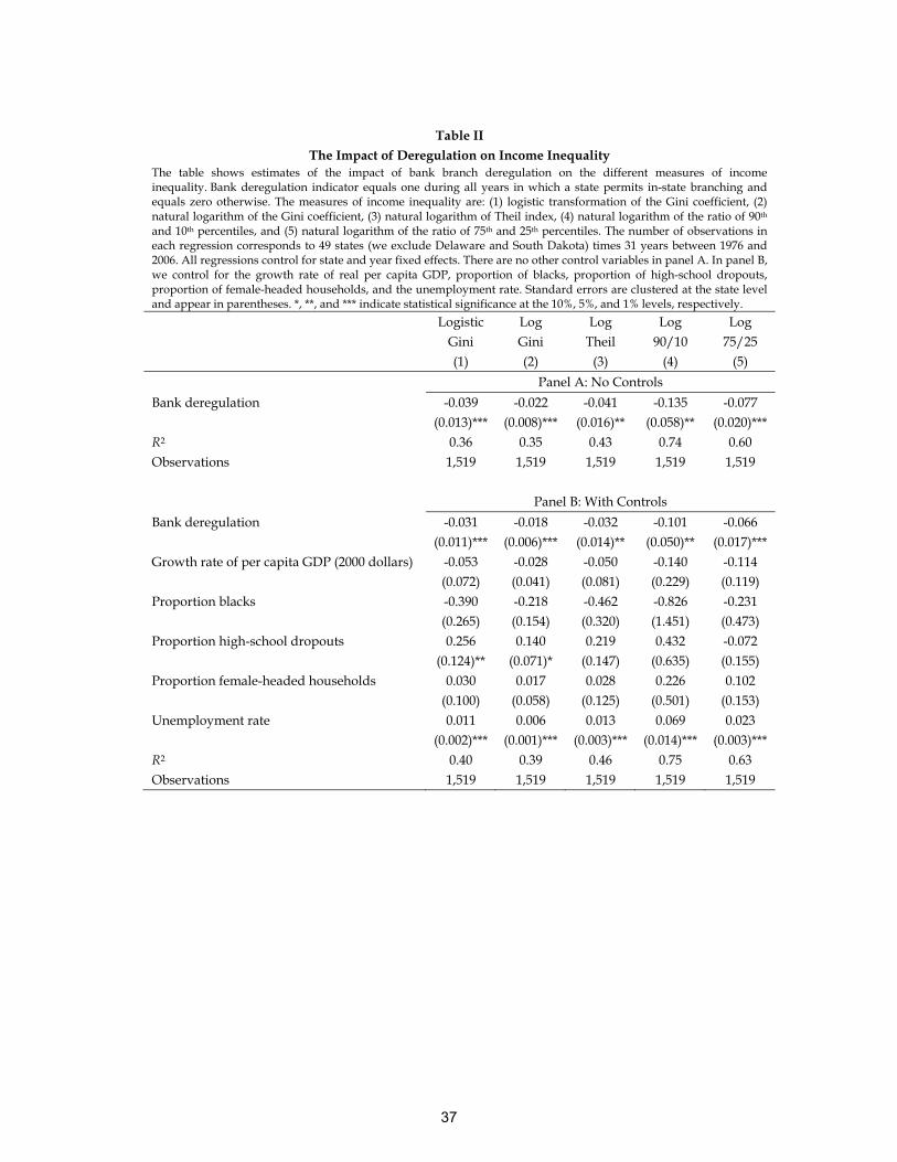
Table II

The Impact of Deregulation on Income Inequality The table shows estimates of the impact of bank branch deregulation on the different measures of income inequality. Bank deregulation indicator equals one during all years in which a state permits in-state branching and equals zero otherwise. The measures of income inequality are: (1) logistic transformation of the Gini coefficient, (2) natural logarithm of the Gini coefficient, (3) natural logarithm of Theil index, (4) natural logarithm of the ratio of 90th and 10th percentiles, and (5) natural logarithm of the ratio of 75th and 25th percentiles. The number of observations in each regression corresponds to 49 states (we exclude Delaware and South Dakota) times 31 years between 1976 and 2006. All regressions control for state and year fixed effects. There are no other control variables in panel A. In panel B, we control for the growth rate of real per capita GDP, proportion of blacks, proportion of high-school dropouts, proportion of female-headed households, and the unemployment rate. Standard errors are clustered at the state level and appear in parentheses. *, **, and *** indicate statistical significance at the 10%, 5%, and 1% levels, respectively.

Logistic Log Log Log Log

Gini Gini Theil 90/10 75/25

(1) (2) (3) (4) (5)

Panel A: No Controls

Bank deregulation -0.039 -0.022 -0.041 -0.135 -0.077

(0.013)*** (0.008)*** (0.016)** (0.058)** (0.020)***

R2 0.36 0.35 0.43 0.74 0.60 Observations 1,519 1,519 1,519 1,519 1,519

Panel B: With Controls

Bank deregulation -0.031 -0.018 -0.032 -0.101 -0.066

(0.011)*** (0.006)*** (0.014)** (0.050)** (0.017)***

Growth rate of per capita GDP (2000 dollars) -0.053 -0.028 -0.050 -0.140 -0.114

(0.072) (0.041) (0.081) (0.229) (0.119)

Proportion blacks -0.390 -0.218 -0.462 -0.826 -0.231

(0.265) (0.154) (0.320) (1.451) (0.473)

Proportion high-school dropouts 0.256 0.140 0.219 0.432 -0.072

(0.124)** (0.071)* (0.147) (0.635) (0.155)

Proportion female-headed households 0.030 0.017 0.028 0.226 0.102

(0.100) (0.058) (0.125) (0.501) (0.153)

Unemployment rate 0.011 0.006 0.013 0.069 0.023

(0.002)*** (0.001)*** (0.003)*** (0.014)*** (0.003)***

R2 0.40 0.39 0.46 0.75 0.63 Observations 1,519 1,519 1,519 1,519 1,519

37

Table III

The Impact of Deregulation on Income Inequality as a Function of Initial State Characteristics

The table presents estimates of the impact of bank deregulation on the logistic transformation of the Gini coefficient of income inequality as a function of initial state characteristics. Bank deregulation equals one during all years in which a state permits in-state branching and equals zero otherwise. All models control for state and year fixed effects. Since we control for state fixed effects the initial state characteristics are dropped from the regressions. Unit banking states are: CO, AR, FL, IL, IA, KS, MN, MO, MT, NE, ND, OK, TX, WI, WV, and WY. Population dispersion equals one divided by population per square mile, which we obtain from the 1960 estimates of U.S. Census Bureau. We use the 1976 values of the share of small banks and small firms in a state, which we obtain from Kroszner and Strahan (1999). These data exclude 12 states that deregulated before 1976. Standard errors are adjusted for state level clustering and appear in parentheses. *, **, and *** indicate statistical significance levels at the 10%, 5%, and 1% levels, respectively. (1) (2) (3) (4)

Bank deregulation -0.022 -0.026 0.026 1.797

(0.014) (0.013)* (0.025) (0.524)***

Deregulation x (unit banking) -0.033

(0.017)*

Deregulation x (initial population dispersion)

-0.313

(0.138)**

Deregulation x (initial share of small banks)

-0.503

(0.189)**

Deregulation x (initial share of small firms)

-2.062

(0.590)***

Linear combination -0.055

(0.017)***

Evaluated at the 25th percentile

-0.029 -0.011 -0.011

(0.013)** (0.016) (0.016)

Evaluated at the 50th percentile

-0.030 -0.029 -0.028

(0.013)** (0.015)* (0.015)*

Evaluated at the 75th percentile

-0.037 -0.043 -0.046

(0.013)*** (0.016)*** (0.015)***

Observations 1,519 1,519 1,147 1,147

38

Table IV

Decomposing the Impact of Deregulation on Income Inequality to Between- and Within-Groups

The table reports the impact of bank branch deregulation on the Theil index of income inequality. Bank deregulation indicator equals one during all years in which a state permits in-state branching and equals zero otherwise. The number of observations in each decomposition is 1,519, corresponding to 49 states (we exclude Delaware and South Dakota) times 31 years between 1976 and 2006. All decompositions control for state and year fixed effects. In panel A, we divide the sample into two mutually exclusive groups: (i) those who are self-employed and (ii) those who work for wages. In panel B we divide the sample of wage workers into two mutually exclusive groups: (i) those with twelve or less years of completed education and (ii) those with thirteen or more years of completed education. In the first column, in both panels, we estimate the overall impact of branch deregulation on the Theil index of inequality using all groups. In the next column, we estimate the impact of deregulation on inequality between the different groups. In the third column, we estimate the impact of deregulation on inequality within the different groups combined. The second and the third columns add up to the first column. In the next columns we estimate the impact of deregulation on income inequality separately within each of the groups. Standard errors are adjusted for state level clustering and appear in parentheses. * and ** indicate statistical significance levels at the 10% and 5% levels, respectively.

Employment Groups:

Panel A: All Workers Total

Between Groups

Within Groups

Self Employed Salaried

Bank deregulation -0.0103 0.0002 -0.0105 -0.0077 -0.0102 (0.0043)** (0.0003) (0.0042)** (0.0074) (0.0042)** Education Groups:

Panel B: Salaried Workers Total

Between Groups

Within Groups

High School or

Less

Some College or

More

Bank deregulation -0.0102 -0.0028 -0.0074 -0.0086 -0.0039

(0.0042)** (0.0011)** (0.0035)** (0.0043)* (0.0038)

39

Table V

The Impact of Deregulation on Earnings Inequality The table shows estimates of the impact of bank branch deregulation on the different measures of earnings inequality. Bank deregulation indicator equals one during all years in which a state permits in-state branching and equals zero otherwise. The measures of earnings inequality are: (1) logistic transformation of the Gini coefficient, (2) natural logarithm of the Gini coefficient, (3) natural logarithm of Theil index, (4) natural logarithm of the ratio of 90th and 10th percentiles, and (5) natural logarithm of the ratio of 75th and 25th percentiles. The number of observations in each regression corresponds to 49 states (we exclude Delaware and South Dakota) times 31 years between 1976 and 2006 times 3 age groups (25-35, 36-45, and 46-54). All regressions control for state and year fixed effects, age fixed effects, age-specific state fixed effects, and age-specific year fixed effects. In panel A, we use total annual earnings of wage and salary workers. In panel B, we use total annual earnings of wage and salary workers, which are conditional on years of completed education. Specifically, we first regress log real annual earnings on six dummies of years of completed education (0-8, 9-11, 12, 13-15, and 16+) and year fixed effects and then calculate measures of inequality based on the residuals. When calculating the residuals we use sampling weights provided by the CPS. Standard errors are clustered at the state level and appear in parentheses. ** and *** indicate statistical significance at the 5% and 1% levels, respectively.

Logistic Log Log Log Log

Gini Gini Theil 90/10 75/25

(1) (2) (3) (4) (5)

Panel A: Unconditional Earnings

Bank deregulation -0.041 -0.025 -0.053 -0.108 -0.054

(0.018)** (0.011)** (0.023)** (0.038)*** (0.020)***

(Bank deregulation) x (Ages 36-45) 0.006 0.004 0.013 0.034 -0.005

(0.015) (0.010) (0.020) (0.036) (0.015)

(Bank deregulation) x (Ages 46-54) 0.011 0.007 0.020 0.034 -0.010

(0.018) (0.012) (0.024) (0.042) (0.018)

R2 0.26 0.26 0.26 0.40 0.39 Observations 4,557 4,557 4,557 4,557 4,557

Panel B: Earnings Conditional on Education

Bank deregulation -0.040 -0.039 -0.083 -0.005 -0.002

(0.015)** (0.015)** (0.031)** (0.002)*** (0.001)**

(Bank deregulation) x (Ages 36-45) 0.004 0.004 0.019 0.001 -0.000

(0.014) (0.014) (0.033) (0.002) (0.001)

(Bank deregulation) x (Ages 46-54) 0.005 0.005 0.016 0.002 -0.001

(0.015) (0.015) (0.034) (0.002) (0.001)

R2 0.50 0.50 0.40 0.48 0.46 Observations 4,557 4,557 4,557 4,557 4,557

40

AL

AR

CO

CT

FL

GA

HI

ILIN

IA

KS

KY

LA

MA

MI

MN

MS

MO MT

NE

NH

NJ

NM

ND

OH

OK

OR

PA

TN

TX

UT

VA

WA

WV

WI

WY

1975

1980

1985

1990

1995

2000

Yea

r of

ban

k d

ere

gula

tion

-.1 -.05 0 .05 .1

Average Gini coefficient prior to bank deregulation

(A)

AL

AR

CO

CT

FL

GA

HI

ILIN

IA

KS

KY

LA

MA

MI

MN

MS

MOMT

NE

NH

NM

ND

OH

OK

OR

PA

TN

TX

UT

VA

WA

WV

WI

WY

1975

1980

1985

1990

1995

2000

Yea

r of

ban

k d

ere

gula

tion

-.02 0 .02 .04

Average change in the Gini coefficient prior to bank deregulation

(B)

Figure 1. Timing of Bank Deregulation and Pre-Existing Income Inequality: Graphical Analysis. Figure (A) shows a scatter plot of the average Gini coefficient of income inequality prior to bank deregulation and the year of bank deregulation. Figure (B) shows a scatter plot of the average change in the Gini coefficient of income inequality prior to bank deregulation and the year of bank deregulation. The t-statistics for the correlations in figures (A) and (B) are 0.20 and -1.16, respectively.

41

-.05

0

.05

.1

.15

Per

cen

tag

e ch

ang

e

5 10 15 20 25 30 35 40 45 50 55 60 65 70 75 80 85 90 95Percentile of income distribution

Significant at 5% Not significant

Figure 2. The Impact of Deregulation on Different Percentiles of Income Distribution. Each bar in the figure represents the estimated impact of bank deregulation on a natural logarithm of a specific percentile of income distribution. Dark bars represent estimates significant at 5% after adjusting the standard errors for clustering. Light bars represent statistically insignificant estimates. Specifically, we report the estimates of γ from 19 separate regressions of the following form:

Y(i)st = α + γDst + As +Bt + εst where Y(i)st is the natural logarithm of ith percentile of income distribution in state s and year t. Dst is a dummy variable which equals to zero prior to bank deregulation and equals to one afterwards. As and Bt are vectors of state and year dummy variables that account for state and year fixed effects, respectively. Each of the 19 regressions has 1,519 observations corresponding to 49 states (we exclude Delaware and South Dakota) times 31 years between 1976 and 2006.

42

-.06

-.04

-.02

0

.02

.04

Per

cen

tag

e ch

ang

e

-10 -5 0 5 10 15Years relative to branch deregulation

Figure 3. The Dynamic Impact of Deregulation on Gini Coefficient of Income Inequality. The figure plots the impact of intrastate bank deregulation on the natural logarithm of the Gini coefficient of income inequality. We consider a 25 year window, spanning from 10 years before deregulation until 15 years after deregulation. The dashed lines represent 95% confidence intervals, adjusted for state-level clustering. Specifically, we report estimated coefficients from the following regression:

log(Gini)st = α + β1D-10st + β2D-9st + … + β25D+15st + As +Bt + εst The D’s equal zero, except as follows: D-j equals one for states in the jth year before deregulation, while D+j equals one for states in the jth year after deregulation. We exclude the year of deregulation, thus estimating the dynamic effect of deregulation on the different percentiles of income distribution relative to the year of deregulation. As and Bt are vectors of state and year dummy variables that account for state and year fixed effects, respectively.

43

-.06

-.03

0

.03

.06

.09

.12

Per

cen

tag

e ch

ang

e in

re

lativ

e r

eal w

age

s

-10 -5 0 5 10 15Years relative to branch deregulation

Figure 4. The Impact of Deregulation on the Relative Wages of Unskilled Workers. The figure shows the dynamic impact of branch deregulation on log real wages of unskilled workers relative to skilled workers. Unskilled workers are those with 12 or less years of completed education. Skilled workers are those with 13 or more years of completed education. The impact of deregulation on relative wages is represented by connected circles; dashed “arms” around the circles represent 95% confidence intervals, adjusted for state level clustering. All estimates are relative to the year of deregulation. Specifically, we report estimated coefficients from the following regression:

r(w)ist = α + β1D-10st + β2D-9st + … + β25D+15st + As +Bt + εst where rist is log real relative wages of unskilled worker i, who resides in states s in year t. Relative wages are obtained as explained in equations (4) and (5). The D’s equal zero, except as follows: D-j equals one for states in the jth year before deregulation, while D+j equals one for states in the jth year after deregulation. We exclude the year of deregulation, thus estimating the dynamic effect of deregulation on the relative wages relative to the year of deregulation. As and Bt are vectors of state and year dummy variables that account for state and year fixed effects, respectively.

44

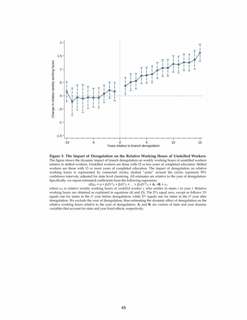
-1.5

-1

-.5

0

.5

1

1.5

2

Cha

nge

in r

ela

tive

we

ekly

wo

rkin

g h

our

s

-10 -5 0 5 10 15Years relative to branch deregulation

Figure 5. The Impact of Deregulation on the Relative Working Hours of Unskilled Workers. The figure shows the dynamic impact of branch deregulation on weekly working hours of unskilled workers relative to skilled workers. Unskilled workers are those with 12 or less years of completed education. Skilled workers are those with 13 or more years of completed education. The impact of deregulation on relative working hours is represented by connected circles; dashed “arms” around the circles represent 95% confidence intervals, adjusted for state level clustering. All estimates are relative to the year of deregulation. Specifically, we report estimated coefficients from the following regression:

r(h)ist = α + β1D-10st + β2D-9st + … + β25D+15st + As +Bt + εst where rist is relative weekly working hours of unskilled worker i, who resides in states s in year t. Relative working hours are obtained as explained in equations (4) and (5). The D’s equal zero, except as follows: D-j equals one for states in the jth year before deregulation, while D+j equals one for states in the jth year after deregulation. We exclude the year of deregulation, thus estimating the dynamic effect of deregulation on the relative working hours relative to the year of deregulation. As and Bt are vectors of state and year dummy variables that account for state and year fixed effects, respectively.

45

-.03

-.02

-.01

0

.01

Pe

rce

nta

ge c

han

ge

-10 -5 0 5 10 15Years relative to branch deregulation

Figure 6. The Impact of Deregulation on Unemployment Rate. The figure shows the dynamic impact of branch deregulation on unemployment rate. The impact of deregulation on unemployment rate is represented by connected circles; dashed “arms” around the circles represent 95% confidence intervals, adjusted for state level clustering. All estimates are relative to the year of deregulation. Specifically, we report estimated coefficients from the following regression:

Log(unemployment)st = α + β1D-10st + β2D-9st + … + β25D+15st + As +Bt + εst where unemploymentst is unemployment rate in state s in year t. The D’s equal zero, except as follows: D-j equals one for states in the jth year before deregulation, while D+j equals one for states in the jth year after deregulation. We exclude the year of deregulation, thus estimating the dynamic effect of deregulation on unemployment rate relative to the year of deregulation. As and Bt are vectors of state and year dummy variables that account for state and year fixed effects, respectively.

46