Bifurcation theory - Alpen-Adria-Universität KlagenfurtPublications... · These parameters...

Christian Pötzsche

Bifurcation theory∗

Lecture NotesSS 2010TU München

July 29, 2011

∗Draft: Corrections are welcome!

2

Christian PötzscheCentre for Mathematical SciencesMunich University of TechnologyBoltzmannstraße 3D-85748 GarchingGermany

[email protected]://www-m12.ma.tum.de/poetzsche

Preface

Mathematical modeling of phenomena in applied sciences like physics, biologyor engineering typically leads to equations depending on one or several param-eters, which are allowed to vary over specified sets (the parameter space or set).These parameters describe how the environment influences a system, and thus,a well-designed system should be robust: This means that small fluctuations inthe parameters do not change its qualitative behavior. However, if the fluctua-tions become larger, the behavior of a system might change in the sense that thenumber or stability property of particular solutions varies. Roughly speaking, theparameters thresholds where such changes occur are called bifurcation values.For a complete understanding of a system it is essential to know these bifurca-tion values, as well as parameter ranges in which there is no essential change.

Let us put these introductory remarks into a more precise framework: Supposethat a given equation

G(x,λ) = 0 (0.0a)

depends on a parameter λ and has a solution (x0,λ0). What can be said about thestructure of the solution set

Sλ := x : G(x,λ) = 0

for parameters λ 6= λ0? The word "structure" can refer to the number of its ele-ments, its topological structure, or properties of its elements (e.g. symmetry orstability). Geometrically one illustrates such changes using the bifurcation dia-gram depicting the set (see Fig. 0.1)

S := (λ, x) : G(x,λ) = 0 .

Continuation methods provide conditions under which Sλ does not changeessentially. This means x0 can be continued along the parameter λ, i.e. there ex-ists a (smooth) unique function x(λ) such that

v

vi Preface

λ

λ1 λ2 λ3

Sλ1

x

Fig. 0.1 Bifurcation diagram of (0.0a)

x(λ0) = x0, Sλ = x(λ)

(see Fig. 0.2(left)). For smooth G the implicit mapping theorem is a well-knowntool to obtain such continuation results. In contrast, bifurcation or branchingmethods describe situations where a unique continuation is not possible, andspecify the structure of the sets Sλ.

Admittedly, until now we have been very vague about the mathematical formof equation (0.0a). In order to tackle this, the following examples illustrate thata surprisingly large number of problems can be cast as (0.0a). The first one ad-dresses the continuation of simple zeros for polynomials:

λλ

x x

λ λ

Sλ

Sλ(λ0, x0)

x(λ)

Fig. 0.2 left: Solution set Sλ does not change under variation of λ. right: Fold bifurcation

Example 0.0.1 (continuation of roots). Let us abbreviate λ := (µ0, . . . ,µm) ∈ Rm+1

for some m ∈N. We are interested in a real polynomial

G(x,λ) :=m∑

n=0µn xn

in x of degree m. Suppose that for an (m +1)-tuple of coefficients λ0 = (µ00, . . . ,µ0

m)the polynomial G(x,λ0) has a simple root x0 ∈R, in particular G(x0,λ0) = 0. Thus,

Preface vii

we can write G(x,λ0) = (x − x0)q(x) with a polynomial q of degree m − 1 andq(x0) 6= 0. Differentiation yields

∂G

∂x(x,λ0) = q(x)+ (x −x0)q ′(x)

and consequently ∂G∂x (x0,λ0) = q(x0) 6= 0. Hence, the implicit mapping theorem im-

plies that there exists an ε> 0 and a smooth function x : Bε(λ0) →R such that

• x(λ0) = x0

• every x(λ), λ ∈ Bε(λ0) ⊆ Rm+1 is a simple root of the polynomial G(x,λ) = 0,which is unique in a neighborhood of x0.

We have shown that simple roots of polynomials depend smoothly on the co-efficients. For roots of higher multiplicity this property needs not to be true.

Example 0.0.2 (fold bifurcation). If the mapping G :R×R→R is given by

G(x,λ) := x2 −λ,

then we immediately obtain (see Fig. 0.2(right))

Sλ :=

;, λ< 0,

0, λ= 0,−pλ,

pλ

, λ> 0.

Obviously, λ= 0 is a bifurcation value in the sense that the number of solutions to(0.0a) changes from 0 for λ < 0, to 1 for λ = 0 and finally to 2 for positive param-eters λ. The pair (0,0) is a so-called fold point. Note that we have ∂G

∂x (0,0) = 0 andtherefore the implicit mapping theorem is not applicable to (0.0a) in (0,0).

Example 0.0.3 (transcritical bifurcation). The so-called logistic mapping definedby the scalar difference equation

xk+1 =λxk (1−xk ) (0.0b)

is a prime example of a discrete dynamical system featuring chaotic behavioron the interval [0,1]. We investigate how the number of equilibria (fixed points)changes under variation of λ. For this purpose we define a mapping G : R×R→ R

by G(x,λ) = λx(1− x)− x and obtain that 0 is a fixed point of (0.0b) resp. a zeroof G(·,λ) for all parameters λ — the trivial branch of fixed points resp. solutions.Moreover, we easily deduce

Sλ :=

0 , λ ∈ 0,1 ,0,1− 1

λ

, λ ∈ (0,4] \ 1

(see Fig. 0.3(left)). Here, the parameters λ = 0 and λ = 1 are bifurcation values inthe sense that the number of fixed points for (0.0b) changes from 1 to 2 under vari-

viii Preface

ation of λ. We have ∂G∂x (x,λ) = λ− 1− 2λx and thus ∂G

∂x (0,0) = ∂G∂x (0,1) = 0; this

means the implicit mapping theorem is not applicable in the points (0,0), (0,1).While a bifurcation from infinity occurs at λ= 0 (the point 1− 1

λ is not defined), forλ= 1 one observes a transcritical bifurcation point (0,1).

It is also possible to interpret the bifurcation value λ= 1 from a dynamical sys-tems perspective. Indeed, the trivial fixed point of (0.0b) looses its asymptotic sta-bility to the fixed point 1− 1

λ .

λ

x

λ = 1

r

λ1

λ1 = 0

Fig. 0.3 left: Transcritical bifurcation. right: Pitchfork bifurcation in the radial component

Example 0.0.4 (pitchfork bifurcation). We consider the planar ordinary differen-tial equation (ODE)

r = r (λ1 − r 2),

θ =λ2(0.0c)

in polar coordinates (r,θ) depending on two parameters λ1,λ2 ∈ R. Due to the de-coupled form of (0.0c) is is clear that the periodic solutions are t 7→ (r0,λ2t +θ0)for any θ0 ∈ [0,2π); here, r0 is a solution of the equation

r (λ1 − r 2) = 0. (0.0d)

Let us focus on the solution structure of the algebraic equation (0.0d) first, and wederive

r ∈R : r (λ1 − r 2) = 0=

0 , λ1 ≤ 0,−

√λ1,0,

√λ1

, λ1 > 0

(see Fig. 0.3(right)). Hence, λ1 = 0 is a bifurcation value for (0.0d) at which thenumber of solutions changes from 1 for λ1 ≤ 0 to 3 for λ1 > 0. This point (0,0) isan example of a pitchfork bifurcation point for (0.0d). This pitchfork bifurcationin the radial component (0.0d) has the following consequences for the dynamicalbehavior of the ordinary differential equation (0.0c):

• In the generic case λ2 6= 0, the trivial solution of (0.0d) bifurcates into a nontriv-

ial∣∣∣ 2πλ2

∣∣∣-periodic solution for λ1 > 0, which does not exist for λ1 ≤ 0. This means

Preface ix

that (0.0c) has a so-called Hopf bifurcation at λ1 = 0. Such Hopf bifurcationscan be interpreted as pitchfork bifurcations in the radial component.

• For λ2 = 0, the trivial solution of (0.0d) bifurcates into a manifold of equilibria(x, y) ∈R2 : x2 + y2 =λ1

for λ1 > 0, which does not exist for λ1 < 0.

Dynamically, the trivial equilibrium looses its asymptotic stability as λ1 increasesthrough the value 0, while the periodic solution (resp. manifold of equilibria) be-comes the global attractor of the system (0.0c) for λ1 > 0.

λ1

x

y

Fig. 0.4 Dynamic bifurcation diagram for a Hopf bifurcation with λ2 < 0

The above Ex. 0.0.4 is qualitatively different from the previous ones, since thebifurcating object was a periodic solution rather than an equilibrium. Only thedecoupled structure of (0.0c) allowed us to determine the bifurcating solution bysolving the algebraic problem (0.0c). For general planar ODEs this is not possi-ble; then, finding a nontrivial periodic solution means to solve a problem in thefunction space of periodic solutions.

Our final example has a more physical background from structural mechan-ics. However, it also requires to solve a differential equation, i.e. an equation in aBanach space.

Example 0.0.5 (Euler bending). We consider an elastic rod of length L > 0, whichhas one end fixed at the origin of the Euclidean plane with coordinates (x, y). Theother end is able to move along the x-axis and is exposed to a force acting along thex-axis. Our further assumptions are as follows:

• The length of the rod does not chance, i.e. it is incompressible.• The rod lies in the (x, y)-plane, i.e. there is not twisting out of the plane.

We will describe the configuration of the rod using the coordinates (x(s), y(s)) indi-cating a point with distance s ∈ [0,L] from the fixed origin (0,0) along the rod. This

x Preface

L

P = 0 P > 0

Fig. 0.5 Bending of an elastic rod. left: No force P = 0. right: Small force P > 0

arclength parametrization yields the relations

x(s) =∫ s

0cosφ(t )d t , y(s) =

∫ s

0sinφ(t )d t for all s ∈ [0,L],

where φ(s) is the angle between the x-axis and the tangent at the rod in the point(x(s), y(s)) (see Fig. 0.6). If P ≥ 0 denotes the applied force, then the Euler-Bernoullitheory of bending yields the relation

−kφ′(s) = P y(s),

where k > 0 is a material constant of the rod. Differentiating this identity implies

(x(s), y(s))

φ(s)

Fig. 0.6 Bending of an elastic rod

the relation −kφ′′(s) = P y ′(s) = P sinφ(s) and thus φ′′(s)+λsinφ(s) = 0 with theparameterλ= P

k . Due to y(0) = y(L) = 0 we arrive at the nonlinear boundary valueproblem

φ′′(s)+λsinφ(s) = 0,

φ′(0) =φ′(L) = 0(0.0e)

and the simplifying assumption sinφ≈φ yields the Sturm-Liouville problemφ′′(s)+λφ(s) = 0,

φ′(0) =φ′(L) = 0.(0.0f)

As the reader might verify, its unique solution is the trivial one, unless for param-eters λ = λk with λk := (

πkL

)2, k ∈ N0, where we have a one-parameter family of

nontrivial solutions φk (s) = γcos(√λk s), γ ∈ R \ 0. Hence, for the linear prob-

lem the trivial solution bifurcates into infinitely many solutions at the bifurcationvalues λk (see Fig. 0.7(left)).

The nonlinear problem (0.0e) can be tackled using bifurcation theory. Thereto,we formulate it via the abstract equation (0.0a) with

Preface xi

λλ

X X

λ1 λ2 λ3 λ1 λ2 λ3

Fig. 0.7 Bending of an elastic rod. left: Solutions to the linear problem (0.0f). right: Solutions tothe nonlinear problem (0.0e)

G(φ,λ) =φ′′+λsinφ;

however, differing form the above examples, now the mapping G : X ×R→ Y oper-ates between the Banach spaces

X := φ ∈C 2[0,L] : φ′(0) =φ′(L) = 0

,

∥∥φ∥∥X := max

s∈[0,L]

|φ(s)|, |φ′(s)|, |φ′′(s)| ,

Y :=C 0[0,L],∥∥φ∥∥

Z := maxs∈[0,L]

|φ(s)|.

The resulting bifurcation diagram illustrating the numbers of solutions to the non-linear boundary value problem (0.0e) is sketched in Fig. 0.7(right).

The above examples indicate a dichotomy in bifurcation theory: Static or an-alytical bifurcation theory as part of nonlinear analysis is primarily interested inthe existence of solutions to (0.0a), i.e. in the topological structure of the set Sλ.Dynamic bifurcation theory originates from dynamical systems theory and addi-tionally investigates stability properties of solutions to differential or differenceequations. In this setting a bifurcation means a change in the phase portrait, i.e.a loss of structural stability.

These notes formed the basis for a weekly 90 minute course at the MunichUniversity of Technology during the summer term 2010. In order to keep thepreliminaries minimal, the first chapter is devoted to differential calculus in Ba-nach spaces and in particular the implicit mapping theorem. In Chapter 2 weessentially restrict to the basics of local analytical bifurcation theory, however ina general setting of abstract parameter dependent equations in Banach spaces.This is motivated by the fact that differential or difference equations are equa-tions in function spaces. In order to investigate not only constant solutions, wehave to consider such parameter-dependent differentiable mappings betweenBanach spaces. Indeed, the fruitfulness of this approach becomes apparent inChapter 3: We investigate the continuation and bifurcation behavior of boundedentire solutions to nonautonomous difference equations. Continuation is possi-

xii Preface

ble, provided exponential dichotomies are given. On the other hand, the lack ofdichotomies allows us to apply our abstract bifurcation results from Chapter 2.

Static bifurcation theory in a more comprehensive way is treated in variousmonographs on nonlinear analysis, like [Zei93, Chapt. 8]. The monograph [Kie04]is exclusively devoted to various aspects bifurcation theory and contains inter-esting applications to PDEs. A further general and advanced approach is given in[CH96]. On the other hand, a variety of textbooks and monographs on dynamicalsystems deal with dynamic bifurcation theory and we only refer to [Kuz04].

München, July 29, 2011 Christian Pötzsche

Contents

Preface . . . . . . . . . . . . . . . . . . . . . . . . . . . . . . . . . . . . . . . . . . . . . . . . . . . . . . . . . . . . v

1 Continuation . . . . . . . . . . . . . . . . . . . . . . . . . . . . . . . . . . . . . . . . . . . . . . . . . . . . . . 11.1 Analysis in Banach spaces . . . . . . . . . . . . . . . . . . . . . . . . . . . . . . . . . . . . . 11.2 Taylor’s theorem . . . . . . . . . . . . . . . . . . . . . . . . . . . . . . . . . . . . . . . . . . . . . . 61.3 Partial derivatives and Nemytskii operators . . . . . . . . . . . . . . . . . . . . . 101.4 The implicit mapping theorem . . . . . . . . . . . . . . . . . . . . . . . . . . . . . . . . . 14

2 Local bifurcation theory . . . . . . . . . . . . . . . . . . . . . . . . . . . . . . . . . . . . . . . . . . . 232.1 Fredholm operators . . . . . . . . . . . . . . . . . . . . . . . . . . . . . . . . . . . . . . . . . . . 252.2 Lyapunov-Schmidt method . . . . . . . . . . . . . . . . . . . . . . . . . . . . . . . . . . . . 262.3 Fold bifurcation . . . . . . . . . . . . . . . . . . . . . . . . . . . . . . . . . . . . . . . . . . . . . . . 282.4 Bifurcation from simple eigenvalues . . . . . . . . . . . . . . . . . . . . . . . . . . . . 32

3 Application: Nonautonomous bifurcations . . . . . . . . . . . . . . . . . . . . . . . . . . 373.1 Nonautonomous difference equations . . . . . . . . . . . . . . . . . . . . . . . . . . 383.2 Exponential dichotomies . . . . . . . . . . . . . . . . . . . . . . . . . . . . . . . . . . . . . . 423.3 Entire solutions and invariant fiber bundles . . . . . . . . . . . . . . . . . . . . . 493.4 Bifurcation of entire solutions . . . . . . . . . . . . . . . . . . . . . . . . . . . . . . . . . . 54

Solutions to the exercises . . . . . . . . . . . . . . . . . . . . . . . . . . . . . . . . . . . . . . . . . . . . . . . 67

References . . . . . . . . . . . . . . . . . . . . . . . . . . . . . . . . . . . . . . . . . . . . . . . . . . . . . . . . . . . . . 77

Index . . . . . . . . . . . . . . . . . . . . . . . . . . . . . . . . . . . . . . . . . . . . . . . . . . . . . . . . . . . . . . . . . . 79

xiii

xiv Contents

Chapter 1

Continuation

Throughout the whole chapter we suppose that X ,Y are Banach spaces equippedwith a respective norm ‖·‖. Moreover, L(X ,Y ) denotes the Banach space ofbounded linear operators equipped with the norm

‖T ‖ := sup‖x‖=1

‖T x‖ .

1.1 Analysis in Banach spaces

The differential calculus for mappings between arbitrary Banach spaces can befound in various classical monographs like [Die69, AMR88, Lan93, Zei93].

As a matter of course, the derivative provides a linear approximation of a givennonlinear mapping and employs it as primary tool to obtain local informationabout nonlinear smooth problems.

Definition 1.1.1 (Fréchet derivative). Let x be an interior point of a setΩ⊆X . A mapping f : Ω → Y is said to be differentiable in x, if there exists aT ∈ L(X ,Y ), a δ> 0 and a mapping r : Bδ(0) →R such that∥∥ f (x +h)− f (x)−T h

∥∥≤ r (h)‖h‖ for all h ∈ Bδ(0)

and limh→0 r (h) = 0. We denote T as (Fréchet) derivative of f in the point xand write D f (x) := T . If Ω is open and D f (x) exists in every x ∈Ω, then themapping D f :Ω→ L(X ,Y ) is called (Fréchet) derivative of f .

Remark 1.1.2. (1) The derivative of a differentiable mapping f is uniquely de-termined (see [Lan93, p. 334]). Furthermore, if f is differentiable at x, then it iscontinuous in x — in fact, it is even Lipschitz continuous. In order to see this, wechoose δ0 > 0 so small that |r (h)| ≤ 1 for all h ∈ Bδ0 (0) and obtain from the triangle

1

2 1 Continuation

inequality that∥∥ f (y)− f (x)∥∥−∥∥D f (x)(y −x)

∥∥≤∥∥ f (y)− f (x)−D f (x)(y −x)

∥∥≤∥∥y −x

∥∥and consequently

∥∥ f (y)− f (x)∥∥≤ (1+

∥∥D f (x)∥∥)

∥∥y −x∥∥ for all y ∈ Bδ0 (x).

(2) If D f : Ω→ L(X ,Y ) is continuous, we say that f is of class C 1, or write f ∈C 1(Ω,Y ). Inductively, one defines higher oder derivatives

Dn+1 f := D(Dn f

), D0 f := f (1.1a)

and the spaces C m(Ω,Y ) of m-times continuously differentiable mappings. It isconvenient to include the space of continuous functions C 0(Ω,Y ) =C (Ω,Y ) and

C∞(Ω,Y ) :=⋂

m∈NC m(Ω,Y ).

(3) The derivative D f (x) of a mapping f :R→ Y at a real x ∈R is an element ofL(R,Y ), which will be identified with Y by virtue of the isomorphism T 7→ T (1).

(4) The derivative D f (x) of a mapping f :Ω→R in a point x ∈Ω is contained inL(X ,R), i.e., it is a linear bounded functional D f (x) ∈Rd . Here, X ′ denotes the dualspace of X . If X is a Hilbert space with inner product ⟨·, ·⟩, we know from the Rieszrepresentation theorem (see [Lan93, p. 104, Thm. 2.1]) that there exists a uniquevector ∇ f (x) ∈ X such that⟨∇ f (x),ξ

⟩= D f (x)ξ for all ξ ∈ X ;

this vector is called the gradient of f in x.

Example 1.1.3. (1) In the finite-dimensional case X =Rn and Y =Rm the deriva-tive is given by the Jacobian

D f (x) =

∂ f1∂x1

(x) . . . ∂ f1∂xn

(x)...

...∂ fm∂x1

(x) . . . ∂ fm∂xn

(x)

∈Rm×n ,

where f1, . . . , fm :Ω→R denote the components of the mapping f .(2) Let T ∈ L(X ,Y ) and y ∈ Y . Every affine linear mapping f : X → Y given

by f (x) := T x + y is continuously differentiable of arbitrary order with derivativesD f (x) = T and Dm f (x) = 0 for m ≥ 2. In particular, constant mappings are differ-entiable with derivative 0.

(3) The mapping f : L(X ) → L(X ), f (x) := x2 is continuously differentiable withderivative D f (x)y := x y + y x for all x, y ∈ L(X ). This can be seen from the relation∥∥ f (x +h)− f (x)−D f (x)h

∥∥=∥∥(x +h)2 −x2 −xh −hx

∥∥=∥∥h2∥∥≤ r (h)‖h‖

for all x,h ∈ X , when we choose the remainder r (h) = ‖h‖.

Linearity, as well as a product and chain rule also hold in our general setting:

1.1 Analysis in Banach spaces 3

Theorem 1.1.4. Let α,β ∈R and x be an interior point of a set Ω⊆ X .

(a) If f , g :Ω→ Y are differentiable in x, then also the sum α f +βg :Ω→ Yis differentiable in x satisfying the sum rule

D(α f +βg

)(x) =αD f (x)+βDg (x).

(b) Let Y1,Y2 be Banach spaces and · : Y1 × Y2 → Y be a bounded bilinearmapping. If f :Ω→ Y1, g :Ω→ Y2 are differentiable in x, then also f · g :Ω→ Y is differentiable in x satisfying the product or Leibnitz rule

D(

f · g)

(x) = D f (x)g (x)+ f (x)Dg (x). (1.1b)

(c) Let Z be a Banach space and Ω′ ⊆ Z . If g : Ω→ Z is differentiable in xand f : Ω′ → Y is differentiable in the interior point g (x) ∈Ω′, then alsothe composition f g :Ω→ Y is differentiable in x fulfilling the chain rule

D(

f g)

(x) = D f (g (x))Dg (x).

Remark 1.1.5. (1) The above formula for the product rule (1.1b) is a brief notationfor D

(f · g

)(x)ξ= D f (x)ξ · g (x)+ f (x) ·Dg (x)ξ for all ξ ∈ X .

(2) Using mathematical induction the above result can be extended as follows:If f , g are of class C m , then also the linear combination α f +βg , the product f · gand the composition f g are m-times continuously differentiable.

Proof. (a) See [Lan93, p. 335].(b) See [Lan93, p. 336].(c) See [Lan93, p. 337]. ut

Example 1.1.6. Suppose X is a Hilbert space with inner product ⟨·, ·⟩.(1) The mapping f : X → R, f (x) := ‖x‖2 is continuously differentiable. We see

this from the relation f (x) = ⟨x, x⟩. Thereto, due to the Cauchy-Schwarz inequality∣∣⟨x, y⟩∣∣≤ ‖x‖

∥∥y∥∥ for all x, y ∈ X we see that ⟨·, ·⟩ : X ×X →R is a bounded bilinear

mapping. Hence, the product rule implies

D f (x)ξ= ⟨ξ, x⟩+⟨x,ξ⟩ = 2⟨x,ξ⟩ for all x,ξ ∈ X (1.1c)

and obviously D f : X → L(X ,R), D f (x) = 2⟨x, ·⟩ is continuous. Moreover, the gra-dient of f is ∇ f (x) = 2x.

(2) The norm mapping ‖·‖ : X → R is continuously differentiable on X \ 0.Thereto, we write n : X →R, n(x) := ‖x‖ and due to the relation ‖x‖ =

√f (x) (with

f given in (1)) it follows from the chain rule

Dn(x)ξ= D f (x)

2√

f (x)ξ= D f (x)

2‖x‖ ξ(1.1c)=

⟨x

‖x‖ ,ξ

⟩for all x 6= 0, ξ ∈ X .

4 1 Continuation

We can conclude the gradient ∇n(x) = x‖x‖ for all x 6= 0.

In order to formulate the mean value theorem for Banach space-valued func-tions we need an appropriate integral notion. Thereto, let [a,b] be a closed inter-val and a < b be reals. A mapping f : [a,b] → X is called step map, if there exists afinite partition

a := t0 ≤ t1 ≤ . . . ≤ tn ≤ tn+1 := b

and vectors vk ∈ X such that f (t ) ≡ vk on (tk , tk+1) for all k ∈ 0, . . . ,n (seeFig. 1.1(left)). The set S([a,b], X ) of step maps forms a linear subspace of allbounded mappings from [a,b] into X . Moreover, the integral of a step map isdefined as

I ba ( f ) :=

n∑k=0

(tk+1 − tk )vk

and defines a bounded linear functional I ba : S([a,b], X ) → X with

∥∥∥I ba f

∥∥∥≤n∑

k=0(tk+1 − tk )‖vk‖ ≤ (b −a)

∥∥ f∥∥∞ . (1.1d)

Thus, the linear extension theorem (see [Lan93, p. 75, Thm. 3.1]) implies thatthere exists a unique and continuous extension

∫ ba of the linear form I b

a to theclosure clS([a,b], X ), which additionally preserves the norm estimate (1.1d). We

denote∫ b

a : clS([a,b], X ) → X as integral and write∫ b

af =

∫ b

af (t )d t .

In particular, one obtains the inclusion C ([a,b], X ) ⊆ clS([a,b], X ).

a b t

f (t )

t1 t2 tn. . .

Ω

x

x +h

Fig. 1.1 left: Integral of a step function. right: Points x, x+h ∈Ω in Thm. 1.1.7 such that the lineconnecting x and x +h is contained in the domain Ω

The following mean value theorem, also known as Lemma of Hadamard, holdsfor domains Ω containing a line connecting two points x and x +h.

1.1 Analysis in Banach spaces 5

Theorem 1.1.7 (mean value theorem). Let Ω⊆ X be open and suppose thatf : Ω→ Y is continuously differentiable. If x,h ∈ X satisfy x + th ∈Ω for allt ∈ [0,1], then

f (x +h)− f (x) =∫ 1

0D f (x + th)h d t =

∫ 1

0D f (x + th)d th.

Proof. See [Lan93, p. 341, Thm. 4.2]. ut

Corollary 1.1.8 (mean value estimate). One has the estimate∥∥ f (x +h)− f (x)∥∥≤ sup

t∈[0,1]

∥∥D f (x + th)∥∥‖h‖ .

Proof. See [Lan93, p. 342, Cor. 4.3]. ut

Corollary 1.1.9. An open setΩ⊆ X is connected if and only if every differen-tiable mapping f :Ω→ Y satisfying the identity D f (x) ≡ 0 on Ω is constant.

Proof. We have to prove two directions:(⇒) Let f : Ω→ Y be a differentiable function vanishing identically on Ω. We

show that f is constant. Given a fixed x0 ∈Ω the preimage

Ω1 := f −1(

f (x0)) =

x ∈Ω : f (x) = f (x0)

is nonempty (one has x0 ∈Ω1). If x ∈Ω1, then the open set Ω contains a convexneighborhood U of x. Hence, the mean value estimate from Cor. 1.1.8 implies∥∥ f (y)− f (x)

∥∥≤ supt∈[0,1]

∥∥D f (x + t (y −x))∥∥∥∥y −x

∥∥= 0

and therefore f (y) = f (x) = f (x0) for all y ∈U . This shows U ⊆Ω1 andΩ1 is open.On the other hand,Ω1 is also closed since f is continuous. Therefore, the com-

plement Ω2 := Ω \Ω1 must be open. If Ω2 is nonempty, then Ω = Ω1∪Ω2 is thedisjoint union of two open nonempty sets. This contradicts the connectedness ofΩ, thus Ω2 =; and Ω=Ω1.

(⇐) Suppose thatΩ is not connected. Then there exist open nonempty disjointsets Ω1,Ω2 ⊆ X with Ω=Ω1 ∪Ω2. With a nonzero vector y ∈ Y we define

6 1 Continuation

f (x) :=

y, x ∈Ω1,

0, x ∈Ω2

and obtain D f (x) ≡ 0 on Ω. However, f is not constant. ut

Exercises

Exercise 1.1.10. Assume that L(X ) is the Banach algebra of all bounded linearendomorphisms on a Banach space X . Show that

(a) the set GL(X ) ⊆ L(X ) of all invertible mappings in L(X ) is open (and nonempty),(b) the mapping f : GL(X ) → L(X ), f (x) = x−1 is differentiable with derivative

D f (x)ξ=−x−1ξx−1 for all x ∈GL(X ), ξ ∈ L(X ).

Exercise 1.1.11. Let X ,Y be Banach spaces,Ω⊆ X be open and L ≥ 0. Prove that adifferentiable mapping f :Ω→ Y satisfying a global Lipschitz condition∥∥ f (x)− f (y)

∥∥≤ L∥∥x − y

∥∥ for all x, y ∈Ω.

fulfills the estimate∥∥D f (x)

∥∥≤ L for all x ∈Ω.Hint: Rem. 1.1.2(1)

Exercise 1.1.12. Let X ,Y be Banach spaces, Ω ⊆ X be open and suppose thatf : Ω→ Y is differentiable in x ∈ Ω and completely continuous.1 Verify that thederivative D f (x) ∈ L(X ,Y ) is a compact2 linear operator.Hint: Proceed indirectly and assume D f (x)B1(0) ⊆ Y is not relatively compact.

1.2 Taylor’s theorem

While the derivative D f of a (nonlinear) mapping f serves as linear substitute,it is sometimes desirable to have better approximations at hand. They involvehigher order derivatives Dn f as recursively defined in (1.1a). Let us recapitulatethe corresponding construction:

Given an openΩ⊆ X we consider a sufficiently smooth mapping f :Ω→ Y . Itsfirst order derivative, say in x0 ∈Ω, is a bounded linear mapping D f (x0) ∈ L(X ,Y ).The second order derivative D2 f (x0) is defined to be the derivative of x 7→ D f (x)in x0, i.e., we have the inclusion D2 f (x0) ∈ L(X ,L(X ,Y )) and inductively

Dn f (x0) ∈ L(. . . ,L

(X ,L(X ,L(X ,Y ))

)).

1 this means f :Ω→ Y is continuous and for each bounded subset B ⊆Ω the image f (B) ⊆Ω isrelatively compact2 a linear operator T ∈ L(X , y) is called compact, if the image T B1(0) ⊆ Y is relatively compact

1.2 Taylor’s theorem 7

This cumbersome notation can be avoided by introducing the following spaces:

Definition 1.2.1. Let n ∈N and X1, . . . , Xn , Y be Banach spaces. A mappingT : X1 × . . .×Xn → Y is called n-linear bounded, if

(i) T is linear in each argument x1 to xn ,(ii) there exists a C ≥ 0 such that the estimate ‖T x1 · · ·xn‖ ≤ C

∏ni=1 ‖xi‖

holds for all x1 ∈ X1, . . . , xn ∈ Xn .

The space of all n-linear bounded mappings is denoted by L(X1, . . . , Xn ,Y ).For X = X1 = . . . = Xn we denote an n-linear bounded mapping T : X n → Yas symmetric, if

T x1 · · ·xn = T xσ(1) · · ·xσ(n) for all x1, . . . , xn ∈ X

holds for every permutation σ : 1, . . . ,n → 1, . . . ,n. The space of all sym-metric n-linear bounded mappings is denoted by Ln(X ,Y ).

Remark 1.2.2. (1) An n-linear mapping is also called multilinear. For a symmetricmultilinear mapping T ∈ Ln(X ,Y ) we often abbreviate

T xn := T x · · ·x︸︷︷︸n-times

and sometimes it is convenient to write L0(X ,Y ) := Y .(2) The space L(X1, . . . , Xn ,Y ) is a Banach space w.r.t. the norm

‖T ‖ := sup‖x1‖,...,‖xn‖≤1

‖T x1 · · ·xn‖

and we consider Ln(X ,Y ) as a subspace of L(X , . . . , X ,Y ).

It is common practice to identify the spaces

L(X ,L(X ,Y )) ∼= L(X , X ,Y ) = L2(X ,Y ), T x1x2 7→ (T x1)x2,

L(X ,L(X ,L(X ,Y ))

)∼= L(X , X , X ,Y ) = L3(X ,Y ), T x1x2x3 7→ ((T x1)x2)x3, . . .

and in this sense the mth derivative is a symmetric multilinear form:

Proposition 1.2.3. Let Ω ⊆ X be open. If f ∈ C m(Ω,Y ), then one hasDn f (x) ∈ Ln(X ,Y ) for all x ∈Ω and 1 ≤ n ≤ m.


Example 1.2.4. (1) Let X = Rd and Y = R. If f : Ω→ R is two-times continuouslydifferentiable in x ∈Ω, then D f (x) ∈ L(Rd ,R) ∼=R1×d with

8 1 Continuation

D f (x)ξ= ⟨∇ f (x),ξ⟩= d∑

i=1

∂ f

∂xi(x)ξi for all ξ ∈Rd .

For the second order derivative D2 f (x) ∈ L2(Rd ,R) we obtain the representation

D2 f (x)ξη= ⟨H(x)ξ,η

⟩= d∑i , j=1

ξi∂2 f

∂xi∂x j(x)η j for all ξ,η ∈Rd

with the Hessian H(x) := ( ∂2 f∂xi ∂x j

(x))

1≤i , j≤d .

(2) For the mapping f :R2 →R2 given by f (x) :=(

a20x21+a11x1x2+a02x2

2

b20x21+b11x1x2+b02x2

2

)we obtain

the derivatives

D f (x)ξ=(2a20x +a11x2 a11x +2a02x2

2b20x +b11x2 b11x +2b02x2

)(ξ1

ξ2

)=

((2a20x +a11x2)ξ1 + (a11x +2a02x2)ξ2

(2b20x +b11x2)ξ1 + (b11x +2b02x2)ξ2

),

D2 f (x)ξη=(2a20ξ1 +a11ξ2 a11ξ1 +2a02ξ2

2b20ξ1 +b11ξ2 b11ξ1 +2b02ξ2

)(η1

η2

)=

((2a20ξ1 +a11ξ2)η1 + (a11ξ1 +2a02ξ2)η2

(2b20ξ1 +b11ξ2)η1 + (b11ξ1 +2b02ξ2)η2

)and Dn f (x) = 0 ∈ Ln(R2,R2) for all x,ξ,η ∈R2, n > 2.

After these preparations we finally arrive at Taylor’s theorem. Note that it re-duces to the mean value Thm. 1.1.7 for C 1-mappings.

Theorem 1.2.5 (Taylor). Let Ω⊆ X be open and suppose that f :Ω→ Y is ofclass C m . If x,h ∈ X satisfy x + th ∈Ω for all t ∈ [0,1], then

f (x +h) =m−1∑n=0

1

n!Dn f (x)hn +Rm(x,h) =

m∑n=0

1

n!Dn f (x)hn + rm(x,h)

with remainders Rm(x,h) = ∫ 10

(1−t )m−1

(m−1)! Dm f (x + th)d thm and rm satisfying

‖rm(x,h)‖ ≤ 1

m!sup

t∈[0,1]

∥∥Dm f (x + th)−Dm f (x)∥∥‖h‖m

and limh→0rm (x,h)‖h‖m = 0.

Proof. See [Lan93, pp. 349–350]. ut

1.2 Taylor’s theorem 9

Exercises

Exercise 1.2.6. Let X be a Banach space and F : X → R be continuously differen-tiable. Suppose there exists an x0 ∈ X and an ε> 0 with

F (x0) ≤ F (x) for all x ∈ Bε(x0),

i.e. x0 is a local minimum of F . Show that DF (x0) = 0!

Exercise 1.2.7 (fundamental lemma in the calculus of variations). Let a < b bereals and f ∈C m[a,b] for some m ∈N0. Show that∫ b

af (t )ψ(t )d t = 0 for all ψ ∈C m

0 [a,b]

implies f (t ) ≡ 0 on [a,b], where C m0 [a,b] :=

ψ ∈C m[a,b] : ψ(a) =ψ(b) = 0.

Hint: Try out the test function ψ(t ) := (a − t )(t −b) f (t )!

Exercise 1.2.8. In the following exercises we will successively discuss a fundamen-tal problem in the calculus of variations — we shall derive the so-called Euler-Lagrange equations. They give a necessary condition for the existence of min-ima (or maxima) for smooth functionals. For this purpose, let a < b be reals,g : [a,b]×R2 →R be continuous and define the functional

F (φ) :=∫ b

ag (t ,φ(t ), φ(t ))d t . (1.2a)

Obviously, the mapping F : C 20 [a,b] → R is well-defined. We furthermore assume

that (t , x1, x2) → g (t , x1, x2) is continuously differentiable and possesses continu-

ous partial derivatives ∂i+ j g

∂xi1∂x

j2

: [a,b]×R2 → R for all 0 ≤ i + j ≤ 2. In Ex. 1.3.6 we

will show that F is continuously differentiable with derivative

DF (φ)ψ=∫ b

a

∂g

∂x1(t ,φ(t ), φ(t ))ψ(t )d t +

∫ b

a

∂g

∂x2(t ,φ(t ), φ(t ))ψ(t )d t (1.2b)

for all φ,ψ ∈C 20 [a,b].

Using this information, prove that ifφ0 ∈C 20 [a,b] is a local minimum of F , then

it satisfies the Euler-Lagrange equations

∂g

∂x1(t ,φ0(t ), φ0(t ))− ∂2g

∂t∂x2(t ,φ0(t ), φ0(t ))− ∂2g

∂x1∂x2(t ,φ0(t ), φ0(t ))φ0(t )

−∂2g

∂x22

(t ,φ0(t ), φ0(t ))φ0(t ) = 0.

Hints:

(1)What does Ex. 1.2.6 mean for the mapping F ?

10 1 Continuation

(2)Apply integration by parts to the second summand in (1.2b) and simplify yourresult such that Ex. 1.2.7 can be applied.

1.3 Partial derivatives and Nemytskii operators

We now suppose that a Banach space X = X1× . . .×Xn is the cartesian product ofn ∈N further Banach spaces Xi equipped with the norm3

‖x‖X := nmaxi=1

‖xi‖Xi, (1.3a)

where xi ∈ Xi are the coordinates of x, i.e., x = (x1, . . . , xn). Moreover, let us restrictto subsets Ω⊆ X of the form Ω=Ω1 × . . .×Ωn with (nonempty) sets Ωi ⊆ Xi .

In this set-up, choose a point x ∈ Ω and let us consider mappings f : Ω→ Ysuch that xi ∈Ωi is an interior point for some 1 ≤ i ≤ n. If the derivative of

f (x1, . . . , xi−1, ·, xi+1, . . . , xn) :Ωi → Y

exists in x, it is denoted by Di f (x) ∈ L(Xi ,Y ) and called partial derivative of fin x w.r.t. the i th variable. Correspondingly, for open Ωi one defines the partialderivatives Di f : Ω→ L(Xi ,Y ), as well as higher order and mixed partial deriva-tives.

Theorem 1.3.1. Let Ωi ⊆ Xi be open for all 1 ≤ i ≤ n and m ∈N. A mappingf :Ω→ Y is of class C m if and only if Di f ∈C m−1(Ω,L(Xi ,Y )) holds for every1 ≤ i ≤ n. In this case,

D f (x)ξ=n∑

i=1Di f (x)ξi for all x ∈Ω, ξ= (ξ1, . . . ,ξn) ∈ X .


In the context of higher order and mixed partial derivatives it is convenientto work with multiindices. A multiindex ν is an n-tuple ν = (ν1, . . . ,νn) ∈Nn

0 and|ν| := ν1 + . . .+νn denotes its length. This said, we often write

Dν f (x) = Dν11 · · ·Dνn

n f (x).

3 on products of Hilbert spaces Xi with inner products (·, ·)Xi it is common to use the innerproduct

(x, y) :=n∑

i=1(xi , yi )Xi for all x, y ∈ X

and the induced norm ‖x‖X :=√∑n

i=1 ‖xi ‖2Xi

1.3 Partial derivatives and Nemytskii operators 11

For sufficiently smooth mappings we obtain that partial derivatives commute:

Theorem 1.3.2 (Schwarz). Let Ωi ⊆ Xi be open for 1 ≤ i ≤ n and m ∈N. If amapping f :Ω→ Y is of class C m , then

Dν11 · · ·Dνn

n f (x) = Dνσ(1)σ(1) · · ·D

νσ(n)σ(n) f (x) for all x ∈Ω, ν ∈Nn

0 , |ν| ≤ m

and all permutations σ : 1, . . . ,n → 1, . . . ,n.

Proof. This follows inductively from [Lan93, p. 355, Thm. 7.3]. ut

Of particular importance for our future Sections dealing with applications areso-called Nemytskii or substitution operators on the spaces

`∞(Ω) :=

(φk )k∈Z : φk ∈Ω and supk∈Z

∣∣φk∣∣<∞

,

`0(Ω) :=

(φk )k∈Z : φk ∈Ω and lim|k|→∞

φk = 0

of bounded resp. limit zero sequences with values in a subsetΩ of a Banach spaceX — when dealing with `0(Ω) it is assumed 0 ∈Ω. In this context we use |·| for thenorm on X , while both sequence spaces will be canonically equipped with thesup-norm ∥∥φ∥∥ := sup

k∈Z|φk |.

Consider mappings fk :Rd ×Λ→Rd , k ∈Z, depending on a parameter λ ∈Λ. Theparameter spaceΛ is assumed to be an open convex subset of a Banach space Y .

Hypothesis 1.3.1. Let m ∈N0 and Λ be open convex. Suppose fk : Rd ×Λ→ Rd ,k ∈Z, are C m-mappings such that the following holds for 0 ≤ j ≤ m:

(a) For all bounded B ⊆Rd one has

supk∈Z

supx∈B

∣∣∣D j fk (x,λ)∣∣∣<∞ for all λ ∈Λ

(well-definedness) and for all λ0 ∈Λ and ε> 0 there exists a δ> 0 with∣∣x − y∣∣< δ ⇒ sup

k∈Z

∣∣∣D j fk (x,λ)−D j fk (y,λ0)∣∣∣< ε (1.3b)

for all x, y ∈Rd and λ ∈ Bδ(λ0) (uniform continuity).(b) We have 0 ∈Rd and the limit relation limk→±∞ fk (0,λ) = 0 for all λ ∈Λ.

The availability of Banach space-valued parameters broadens our range forapplications significantly:

12 1 Continuation

Example 1.3.3. (1) Let P ⊆ Rn be open convex and suppose g : Rd ×P → Rd is aC m-mapping. When interested in the behavior of the recursive equation

xk+1 = g (xk , p) (1.3c)

under parameters p varying in k, we define the parameter space Λ := `∞(P ) asopen convex subset of the Banach space `∞(Rn). The mapping fk : Rd ×Λ→ Rd ,fk (x,λ) := g (x,λk ) fulfills Hyp. 1.3.1(a) — one speaks of parametric perturbations.

(2) The scenario of (1) can be extended as follows: When interested in the be-havior of (1.3c) under varying right-hand sides g , one introduces the parameterspace Λ :=

λ ∈C (Z×Rd ,Rd )| sup(k,x)∈Z×Rp |g (k, x)| <∞and equips it with the

norm ‖λ‖ := sup(k,x)∈Z×Rn |λ(k, x)|. Then the appropriate choice to fit Hyp. 1.3.1(a)

is fk :Rd ×Λ→Rd given by fk (x,λ) :=λ(k, x).

Under the above assumptions we formally introduce various Nemytskii oper-ators derived from the functions fk . They are pointwise defined as

N f (φ,λ)k := fk (φk ,λ), N jf (φ,λ)k := D j fk (φk ,λ),

Nυf (φ,λ)k := Dυ1

1 Dυ22 fk (φk ,λ)

for all k ∈ Z. Here, 0 ≤ j ≤ m and the pair υ = (υ1,υ2) ∈ N20 denotes a multiin-

dex of length |υ| := υ1 +υ2 ≤ m. Finally, for the sake of a convenient notation weabbreviate `∞ = `∞(Rd ) and `0 = `0(Rd ).

Lemma 1.3.4. Under Hyp. 1.3.1(a) the operators N jf : `∞×Λ→ `∞(L j (Rd ×Y ,Rd ))

and Nυf : `∞×Λ→ `∞

(Lυ1 (Rd ,Lυ2 (Y ,Rd ))

)are well-defined and continuous.

Proof. Let λ ∈Λ, φ ∈ `∞ and 0 ≤ j ≤ m be given. Due to Hyp. 1.3.1(a) the deriva-tives D j fk (·,λ) map bounded sets into bounded sets uniformly in k ∈ Z. Thus,

also the sequence (D j fk (φk ,λ))k∈Z is bounded and the operator N jf has values

in `∞(L j (Rd ×Y ,Rd )). In order to establish its continuity, we arbitrarily chooseλ∗ ∈Λ and φ∗ ∈ `∞. For every ε > 0 we know from Hyp. 1.3.1(a) that there existsa δ > 0 such that (1.3b) holds. In particular, for sequences φ ∈ Bδ(φ∗)∩`∞ andλ ∈ Bδ(λ∗) one has ∣∣φk −φ∗

k

∣∣≤ ∥∥φ−φ∗∥∥< δ for all k ∈Z

and therefore∣∣D j fk (φk ,λ)−D j fk (φ∗

k ,λ∗)∣∣ < ε for all k ∈ Z. Passing to the least

upper bound over k in this inequality we arrive at∥∥N j

f (φ,λ)− N jf (φ∗,λ∗)

∥∥ ≤ ε

and this proves the continuity of N jf .

Given υ ∈N20, |υ| ≤ m these properties carry over from the operator N j

f given by

the Frechét derivatives of fk to the operator Nυf defined via partial derivatives. ut

Proposition 1.3.5. Under Hyp. 1.3.1(a) the operator N f : `∞ ×Λ → `∞ is well-defined and m-times continuously differentiable on `∞×Λwith partial derivatives

1.3 Partial derivatives and Nemytskii operators 13

DυN f (φ,λ) = Nυf (φ,λ) for all φ ∈ `∞, λ ∈Λ, |υ| ≤ m. (1.3d)

If also Hyp. 1.3.1(b) is satisfied, then the same holds for N f : `0 ×Λ→ `0.

Proof. It follows from Lemma 1.3.4 with j = 0 that N f : `∞ ×Λ → `∞ is well-

defined. Concerning the smoothness assertion, we only establish D j N f = N jf .

For this, let φ∗ ∈ `∞, λ∗ ∈Λ and φ ∈ `∞, λ ∈ Y sufficiently small that λ∗+λ ∈Λ.For every 0 ≤ j < m we define the real-valued remainder

r j (φ,λ) := suph∈[0,1]

∥∥∥N j+1f (φ∗+hφ,λ∗+hλ)−N j+1

f (φ∗,λ∗)∥∥∥

and the continuity for N j+1f from Lemma 1.3.4 yields lim(φ,λ)→(0,0) r j (φ,λ) = 0.

After these preparations, the mean value Thm. 1.1.7 implies∣∣∣∣D j fk (φ∗k +φk ,λ∗+λ)−D j fk (φ∗

k ,λ)−D j+1 fk (φ∗k ,λ∗)

(φk

λ

)∣∣∣∣≤

∫ 1

0

∣∣∣D j+1 fk (φ∗k +hφk ,λ∗+hλ)−D j+1 fk (φ∗

k ,λ∗)∣∣∣ dh

∣∣∣∣(φk

λ

)∣∣∣∣(1.3a)≤ r j (φ,λ)max

∥∥φ∥∥ , |λ| for all k ∈Z

and passing over to the least upper bound for k ∈Z yields∥∥∥∥N jf (φ∗+φ,λ∗+λ)−N j

f (φ∗,λ∗)−N j+1f (φ∗,λ∗)

(φ

λ

)∥∥∥∥≤ r j (φ,λ)max∥∥φ∥∥ , |λ| .

Sinceφ∗ ∈ `∞,λ∗ ∈Λwere arbitrary, N jf is differentiable on `∞×Λwith derivative

N j+1f and mathematical induction shows that N f is m-times differentiable with

D j N f = N jf for 0 ≤ j ≤ m. Finally, Dm N f is continuous by Lemma 1.3.4.

It remains to show the assertion when N f is defined on `0 ×Λ. Given a se-quence φ∗ ∈ `0, we deduce from Hyp. 1.3.1 that

Cλ := supk∈Z

sups∈[0,1]

∣∣D1 fk (sφ∗k ,λ)

∣∣<∞ for all λ ∈Λ.

Therefore, the mean value estimate from Cor. 1.1.8 yields∣∣ fk (φ∗k ,λ)

∣∣= ∣∣ fk (φ∗k ,λ)− fk (0,λ)

∣∣+ ∣∣ fk (0,λ)∣∣≤Cλ

∣∣φ∗k

∣∣+ ∣∣ fk (0,λ)∣∣ for all λ ∈Λ;

thus, the right-hand side of this estimate tends to 0 as k →±∞. Hence, the Ne-mytskii operator N f : `0 ×Λ→ `0 is well-defined and the corresponding smooth-ness assertions for N f follow as above. ut

As a closing remark we point out that quite similar results also hold for Nemyt-skii operators N f (φ)(t ) := f (t ,φ(t ),λ) between function spaces

14 1 Continuation

BC (R,Ω) :=φ ∈C (R,Ω)| sup

t∈R|φ(t )| <∞

,

BC0(R,Ω) :=φ ∈C (R,Ω)| lim

t→±∞φ(t ) = 0

rather than sequence spaces, provided the function f : R×Ω×Λ→ Rd satisfiesassumptions analogous to Hyp. 1.3.1.

Exercises

Exercise 1.3.6. Let F : C 1[a,b] → R be the integral operator defined previously in(1.2a), where we use the norm∥∥φ∥∥ := sup

t∈[a,b]

|φ(t )|, |φ(t )|on C 1[a,b]. Moreover, suppose the partial derivatives D2g ,D3g : [a,b]×R2 → R ofa continuous function g : [a,b]×R2 → R exist and are continuous. Prove that F iscontinuously differentiable and determine its derivative DF .

Exercise 1.3.7. Given a real γ≥ 0 we define the Banach spaces

Xγ :=φ ∈C [0,∞) : sup

t≥0|φ(t )|e−γt <∞

,

∥∥φ∥∥γ := sup

t≥0|φ(t )|e−γt

and the analytical function f :R→R, f (x) := sin x. Show that the Nemytskii oper-ator F : Xγ → Xγ, F (φ) := sinφ(·) is differentiable for γ= 0. Is F also differentiablefor exponents γ> 0?

1.4 The implicit mapping theorem

The implicit mapping theorem is one of the central pillars in analytical bifurca-tion theory. In order to prove it, some refinements of the contraction mappingprinciple are required. In particular, we need results guaranteeing a smooth de-pendence of fixed points on parameters.

Our first result holds for mappings defined on complete metric spaces Ω, butfor convenience we suppose that Ω is a closed subset of a Banach space X .

Lemma 1.4.1. Let L ∈ [0,1), Ω ⊆ X be closed and Λ be a metric space. If amapping T :Ω×Λ→Ω satisfies

‖T (x,λ)−T (x,λ)‖ ≤ L ‖x − x‖ for all x, x ∈Ω, λ ∈Λ,

1.4 The implicit mapping theorem 15

then the following holds true:

(a) For every λ ∈Λ there exists a unique x∗(λ) ∈Ω with x∗(λ) = T (x∗(λ),λ).(b) The fixed point mapping x∗ :Λ→Ω is continuous, provided T (x, ·) is con-

tinuous for all x ∈Ω.

Proof. See Ex. 1.4.11. ut

Theorem 1.4.2 (uniform contraction principle). Let m ∈ N0, L ∈ [0,1) andΩ⊆ X ,Λ⊆ Y be open. If a mapping T : Ω×Λ→ Ω satisfies T ∈C m(Ω×Λ, X )and

‖T (x,λ)−T (x,λ)‖ ≤ L ‖x − x‖ for all x, x ∈ Ω, λ ∈Λ, (1.4a)

then for every λ ∈Λ there exists a unique x∗(λ) ∈ Ω with x∗(λ) = T (x∗(λ),λ)and the fixed point mapping fulfills x∗ ∈C m(Λ, X ).

Proof. Let λ0 ∈Λ and choose δ> 0 so small that Bδ(λ0) ⊆Λ.(I) From Lemma 1.4.1 we see that there exists a unique fixed point x∗(λ0) ∈Ω

of T (·,λ0) and that x∗ :Λ→ Ω is continuous. For every vector h ∈ Bδ(0) we define∆(h) := x∗(λ0 +h)−x∗(λ0). Indeed, as in the proof of Lemma 1.4.1 one shows

‖∆(h)‖ ≤ 1

1−L

∥∥T (x∗(λ0),λ0 +h)−T (x∗(λ0),λ0)∥∥

and using the mean value estimate from Cor. 1.1.8 that

‖∆(h)‖ ≤ C

1−L‖h‖ for all h ∈ Bδ(0) (1.4b)

with C := supt∈[0,1] ‖D2T (x∗(λ0),λ0 + th)‖. Due to the Lipschitz estimate (1.4a)we know from Ex. 1.1.11 that

‖D1T (x,λ)‖ ≤ L < 1 for all x ∈Ω, λ ∈Λ. (1.4c)

Thus, again Lemma 1.4.1 implies that there is a unique solution T1(λ0) ∈ L(Y , X )to the operator equation

T1 = D1T (x∗(λ0),λ0)T1 +D2T (x∗(λ0),λ0) (1.4d)

and the fixed point mapping T1 :Λ→ L(Y , X ) is continuous.(II) We continue the proof of Thm. 1.4.2 and show the continuous differentia-

bility of the fixed point function x∗ :Λ→ X . Using the mean value Thm. 1.1.7,

∆(h)−T1(λ0)h =

16 1 Continuation

= T (x∗(λ0 +h),λ0)−T (x∗(λ0),λ0)++T (x∗(λ0 +h),λ0 +h)−T (x∗(λ0 +h),λ0)−T1(λ0)h =

(1.4d)= T (x∗(λ0 +h),λ0)−T (x∗(λ0),λ0)−D1T (x∗(λ0),λ0)T1(λ0)h ++T (x∗(λ0 +h),λ0 +h)−T (x∗(λ0 +h),λ0)−D2T (x∗(λ0);λ0)h =

=[∫ 1

0D1T (x∗(λ0)+ t∆(h),λ0)−D1T (x∗(λ0),λ0)d t

]∆(h)+

+[∫ 1

0D2T (x∗(λ0 +h),λ0 + th)−D2T (x∗(λ0),λ0)d t

]h +

+D1T (x∗(λ0),λ0)∆(h)−D1T (x∗(λ0),λ0)T1(λ0)h =

=[∫ 1

0D1T (x∗(λ0)+ t∆(h),λ0)−D1T (x∗(λ0),λ0)d t

]∆(h)+

+[∫ 1


]h +

+D1T (x∗(λ0),λ0)(∆(h)−T1(λ0)h) for all h ∈ Bδ(0)

and from this relation we deduce using (1.4c) that

‖∆(h)−T1(λ0)h‖1 ≤

≤ 1

1−L

∥∥∥∥∫ 1

0D1T (x∗(λ0)+ t∆(h),λ0)−D1T (x∗(λ0),λ0)d t

∥∥∥∥‖∆(h)‖+

+ 1

1−L

∥∥∥∥∫ 1


∥∥∥∥‖h‖ ≤

(1.4b)≤[

C

(1−L)2

∫ 1

0

∥∥D1T (x∗(λ0)+ t∆(h),λ0)−D1T (x∗(λ0),λ0)∥∥ d t+

+ 1

1−L

∫ 1

0

∥∥D2T (x∗(λ0 +h),λ0 + th)−D2T (x∗(λ0),λ0)∥∥ d t

]‖h‖ ≤ r (h)‖h‖ ,

where the remainder r : Bδ(0) →R+0 is given by

r (h) := C

(1−L)2 supt∈[0,1]

∥∥D1T (x∗(λ0)+ t∆(h),λ0)−D1T (x∗(λ0),λ0)∥∥+

+ 1

1−Lsup

t∈[0,1]

∥∥D2T (x∗(λ0 +h),λ0 + th)−D2T (x∗(λ0),λ0)∥∥ .

Hence, it remains to establish the limit relation limh→0 r (h) = 0. However, thisfollows due to the continuity of D1T , D2T and x∗. We have established that x∗

is differentiable in λ0 ∈ Λ with derivative T1(λ0), and from step (I) we see thatT1 :Λ→ L(Y , X ) is also continuous.

(III) The inclusion x∗ ∈C m(Λ, X ) can be shown using mathematical induction.We leave the proof to the interested reader. ut

Now we are in a position to establish the main result in this Chapter 1. Thereto,let Z be a further Banach space and we illustrate this result in Fig. 1.2.


λ0

x0

Ω

λ

x

x∗

Bδ(λ0)

Bε(x0)

Fig. 1.2 Continuation of the solution (x0,λ0) to F (x0,λ0) = z0 by means of the smooth functionx∗ : Bδ(λ0) → Bε(x0)

Theorem 1.4.3 (implicit mapping theorem). Let m ∈N, Ω⊆ X ×Y be openand (x0,λ0) ∈Ω, z0 ∈ Z . If a mapping F ∈C m(Ω, Z ) satisfies

(i) F (x0,λ0) = z0,(ii) D1F (x0,λ0) ∈GL(X , Z ),

then there exist δ> 0, ε> 0 and a C m-function x∗ : Bδ(λ0) → Bε(x0) with thefollowing properties:

(a) x∗(λ0) = x0,(b) F (x,λ) = z0 in Bε(x0)×Bδ(λ0) if and only if x = x∗(λ),(c) Dx∗(λ0) =−D1F (x0,λ0)−1D2F (x0,λ0).

Example 1.4.4. We define three mappings Fn : R× R → R, F1(x,λ) := x2 − λ,F2(x,λ) := x2 −λ2 and F3(x,λ) := x3 −λ. In each case one has Fn(0,0) = 0, but dueto D1Fn(0,0) = 0 the assumption (ii) of Thm. 1.4.3 is violated. We have sketchedthe sets F−1

n (0) in Fig. 1.3. Indeed, the equation Fn(x,λ) = 0 cannot be solved w.r.t.x by a unique and smooth function x∗ over λ.

Remark 1.4.5. (1) It can be shown that Thm. 1.4.3 also holds for m =∞. Moreover,if F is analytic in (x0,λ0) then also x∗ is analytic inλ0 (cf. [Zei93, p. 151, Cor. 4.23]).

(2) The implicit mapping Thm. 1.4.3 is constructive, i.e. the solution mappingx∗ : Bδ(λ0) → Bε(x0) can be computed using a simplified Newton scheme

xn+1(λ) := xn(λ)−D1F (x0,λ0)−1 [F (xn(λ),λ)− z0] for all n ∈N, λ ∈ Bδ(λ0)

18 1 Continuation

x

λ

x

λ

x

λ

n = 1 n = 2 n = 3

Fig. 1.3 Preimage F−1n (0) ⊆R2 for the mappings Fn from Ex. 1.4.4

with initial value x1(λ) :≡ x0 (cf. [Zei93, p. 150–151, Thm. 4.B(b)])

Remark 1.4.6 (continuation method). Of particular importance are parameterspaces Λ ⊆ R. In this situation one deduces from the identity F (x∗(λ),λ) = z0 thatthe function x∗ : Bδ(λ0) → X solves an implicit ordinary differential equation

D1F (x∗(λ),λ)x∗(λ) =−D2F (x∗(λ),λ) (1.4e)

w.r.t. the initial condition x∗(λ0) = x0; one denotes (1.4e) as Davidenko differentialequation. However, instead of approaching (1.4e) directly, the solution branch x∗

can be obtained with a predictor-corrector method (see Fig. 1.4): Choose a smallh 6= 0, define the parameter sequence λn :=λ0 +nh and set n = 0.

• Predictor: Compute ξn+1 := xn +∆ with ∆ ∈ X being the solution to

D1F (xn ,λn)∆=−D2F (xn ,λn)

• Corrector: Solve F (xn+1,λn+1) = z0 for xn+1 with starting value ξn+1.

Increase n and return to the predictor step.

Proof. Let λ ∈Λ. We introduce the mapping T :Ω→ X ,

T (x,λ) := x −D1F (x0,λ0)−1 [F (x,λ)− z0]

and observe that x∗(λ) ∈ X is a fixed point of T (·,λ) if and only if F (x∗(λ),λ) = z0.The mapping T has the same smoothness properties as F and we obtain

D1T (x0,λ0) = id−D1F (x0,λ0)−1D1F (x0,λ0) = 0.

Hence, for continuity reasons there exist δ,ε> 0 with Bε(x0)×Bδ(λ0) ⊆Ω so that‖D1T (x,λ)‖ ≤ 1

2 and

‖T (x,λ)−x0‖ = ‖T (x,λ)−T (x0,λ0)‖ ≤ ε for all x ∈ Bε(x0), λ ∈ Bδ(λ0).


λ

x

λn λn+1

ξn+1

xn+1

xn

Fig. 1.4 Predictor-corrector continuation method with an Euler step as predictor

Thus, T : Bε(x0)×Bδ(λ0) → Bε(x0) is well-defined and fulfills the assumptions ofThm. 1.4.2. It yields a unique fixed point function x∗ : Bδ(λ0) → Bε(x0) for T (·,λ)of class C m , which uniquely solves F (·,λ) = z0 in a vicinity of the point x0, i.e.,F (x∗(λ),λ) ≡ z0 on Bδ(λ0). The assertion (c) follows, if we differentiate this iden-tity using the chain rule in Thm. 1.1.4(c) and set λ=λ0. ut

Let Ω ⊆ X and Ω′ ⊆ Y be open sets. A map f : Ω→ Y is called local C m-diff-eomorphism at x0 ∈Ω, if there exist neighborhoods Ω0 ⊆Ω of x0 and Ω′

0 ⊆Ω′ off (x0) such that f : Ω0 → Ω′

0 is bijective and both f , f −1 are of class C m . Clearly,f :R→R, f (x) = x3 is not a C 1-diffeomorphism at 0.

Theorem 1.4.7 (inverse mapping theorem). Let m ∈N, Ω⊆ X be open andx0 ∈Ω. A mapping f ∈C m(Ω,Y ) is a local C m-diffeomorphism at x0, if andonly if D f (x0) ∈GL(X ,Y ). In the latter case it is

D f −1( f (x0)) = D f (x0)−1. (1.4f)

Example 1.4.8. Let I ⊆R be an open interval and consider an ordinary differentialequation

x = g (x)

20 1 Continuation

with a C 1-right hand side g : Rd → Rd satisfying g (0) = 0. Moreover, we supposethat for every h ∈ BC (I ,Rd ) there exists a unique bounded solution φ : I →Rd of4

x = Dg (0)x +h(t ).

In order to apply Thm. 1.4.7 we abbreviate BC := BC (I ,Rd ), BC 1 := BC 1(I ,Rd ).The interested reader verifies that the mapping f : BC 1 → BC , f (φ) := φ− g (φ(·))is of class C 1 with derivative D f (0)ψ= ψ−Dg (0)ψ at 0. Hence, the invertibility ofD f (0) ∈ L(BC 1,BC ) means that for every h ∈ BC there exists a unique ψ ∈ BC 1

with ψ = Dg (0)ψ+ h, which was our assumption. Then the inverse mappingThm. 1.4.7 is applicable and guarantees that for each inhomogeneity h ∈ BC withsmall norm ‖h‖∞ there exists a unique bounded solution φ to the nonlinear ODE

x = g (x)+h(t ).

Proof. (⇐) We define the C m-mapping F :Ω×Y → Y , F (x,λ) = f (x)−λ. Thanks tothe relations F (x0, f (x0)) = 0 and D1F (x0, f (x0)) = D f (x0) ∈ GL(X ,Y ) we deducefrom the implicit mapping Thm. 1.4.3 the existence of a uniquely determinedC m-function x∗ : Bδ( f (x0)) → Bε(x0) such that F (x∗(λ),λ) ≡ 0, i.e. f (x∗(λ)) = λ

for all points λ ∈ Bδ( f (x0)). Thus, x∗ is the inverse function of f .(⇒) Let f : Ω0 → Ω′

0 be a local C m-diffeomorphism at x0. If we introduceg (y) := f −1(y), then f (g (y)) ≡ y on Ω′

0, g ( f (x)) ≡ x on Ω0 and by the chain rulefrom Thm. 1.1.4(c) it follows

D f (g (y))Dg (y) ≡ idY on Ω′0, Dg ( f (x))D f (x) ≡ idX on Ω0;

for y0 = f (x0) it is D f (x0)Dg (y0) = idY , Dg (y0)D f (x0) = idX and therefore theinclusion D f (x0) ∈GL(X ,Y ). Moreover, we obtain the formula (1.4f). ut

Suppose that N is a closed subspace of X . We say that N is (topologically) com-plemented, if there exists a closed subspace M ⊆ X (the topological complement)such that X = N ⊕M and H : N ×M → X , (x, y) 7→ x + y is a homeomorphism.

Given such a topological splitting X = N ⊕M , there exists a unique projectionP : X → X satisfying R(P ) = N , N (P ) = M ; moreover, P is continuous.

Remark 1.4.9. (1) A closed subspace N is topologically complemented, if it hasfinite dimension or codimension.

(2) Every closed subspace N of a Hilbert space is topologically complemented byvirtue of the orthogonal complement

M⊥ := x ∈ X :

⟨x, y

⟩= 0 for all y ∈ M

.

In case N = spanx1, . . . , xn, the corresponding projection onto N is

4 in case I = R this holds under the assumption that Dg (0) ∈ Rd×d has no eigenvalues on theimaginary axis


P x :=n∑

j=1

⟨x j , x

⟩x j .

Theorem 1.4.10 (surjective implicit mapping theorem). Let m ∈N, Ω⊆ X ,Λ ⊆ Y be open and (x0,λ0) ∈Ω×Λ, z0 ∈ Z . If a mapping F ∈ C m(Ω×Λ, Z )satisfies

(i) F (x0,λ0) = z0,(ii) D1F (x0,λ0) ∈ L(X , Z ) is onto with complemented kernel and projection

operator P ∈ L(X ) onto N (D1F (x0,λ0)),

then there exist ρ > 0, neighborhoods U ⊆ R(P ) of 0, V ⊆ N (P ) of z0 and aunique C m-mapping φ : U ×Bρ(λ0) →V satisfying

F (x0 +ξ+φ(ξ,λ),λ) ≡ z0 on U ×Bρ(λ0).

Proof. For convenience we set X1 := N (D1F (x0,λ0)) and X1 is closed, since thederivative D1F (x0,λ0) is continuous. By our assumptions X1 splits X , i.e. we haveX = R(P )⊕ N (P ) with X1 = R(P ) and the topological complement X2 := N (P ).Note that the restriction L := D1F (x0,λ0)|X2 : X2 → Z is bijective. Indeed, Lη = 0for η ∈ X2 implies η ∈ N (D1F (x0,λ0)) = X1 and thus η= 0, i.e. L is one-to-one.

Now define the C m-mapping G(η,ξ,λ) := F (x0+ξ+η,λ) with arguments ξ ∈ X1,η ∈ X2 satisfying x0 +ξ+η ∈Ω and λ ∈Λ. By assumption we have G(0,0,λ0) = z0

and D1G(0,0,λ) = D1F (x0,λ)|X2 = L ∈ GL(X2, Z ). Consequently, due to the im-plicit mapping Thm. 1.4.3 we can solve the equation G(η,ξ,λ) = z0 for η=φ(ξ,λ)and the claim follows. ut

Exercises

Exercise 1.4.11. Prove Lemma 1.4.1.

Exercise 1.4.12. Let m ∈ N, Λ ⊆ Y be open and suppose A ∈ C m(Λ,L(Cd )). Givenλ0 ∈Λ such that µ0 ∈ C is a simple eigenvalue of A(λ0) with corresponding eigen-vector x0 ∈Cd , show that there exist open neighborhoods Λ0 ⊆Λ of λ0, U ⊆C of µ0

and unique C m-functions µ :Λ0 →U , x :Λ0 →Cd such that

(a) (µ(λ0), x(λ0)) = (µ0, x0),(b) A(λ)x(λ) =µ(λ)x(λ) for all λ ∈Λ0,(c) ‖x(λ)‖ ≡ 1 on Λ0.

Hint: Apply the implicit mapping Thm. 1.4.3 to

F (x,µ;λ) :=(

A(λ)x −µx⟨x, x⟩−1

).

Chapter 2

Local bifurcation theory

In general it is difficult to understand the global solution set of a nonlinear equa-tion. For this reason we retreat to a simpler situation and seek for criteria whena small perturbation guarantees that new solutions are generated near a givenone. In fact, we introduce a parameter in order to describe such perturbationsand consider equations of the form

G(x,λ) = 0. (2.0a)

The generic phenomena are that solutions to (2.0a) vanish, or that new solutionsare generated under varying parameters near a given solution. This is the objectof local "bifurcation" or "branching theory".

In this chapter we introduce several essential tools and results from analyticallocal bifurcation theory for Fredholm operators, like Lyapunov-Schmidt reduc-tion and abstract versions of fold, transcritical and pitchfork bifurcations. Mostof them can be found in standard references (cf. e.g. [CH96, Kie04, Zei93]).

Suppose throughout that X ,Y , Z are real Banach spaces and Ω ⊆ X , Λ ⊆ Ydenote nonempty open neighborhoods of x0 ∈ X , λ ∈ Y in the respective spaces.We deal with C m-mappings G :Ω×Λ→ Z , m ∈N, vanishing at (x0,λ0), i.e.

G(x0,λ0) = 0, (2.0b)

and in the implicit mapping Thm. 1.4.3 we have given a sufficient condition thatthe solution x0 can be continued uniquely for parameters λ 6= λ0. The comple-mentary situation (see Fig. 2.1) is tackled now. Indeed, local bifurcation theoryattempts to describe the preimage G−1(0) in a neighborhood of (x0,λ0).

Definition 2.0.13 (bifurcation point). A pair (x0,λ0) ∈Ω×Λ is called bifur-cation point of (2.0a), if there is a convergent sequence (λn)n∈N in Λ withlimit λ0 and distinct solutions x1

n , x2n ∈Ω, n ∈N, to G(x,λn) = 0 satisfying

23

24 2 Local bifurcation theory

limn→∞x1

n = limn→∞x2

n = x0.

λλ

x x

x0x0

λ1 λ2 λ3λ1 λ2 λ3

Fig. 2.1 Solutions near a given solution branch (λ, x0) for (2.0a) (left) and bifurcation in a linearequation (cf. Ex. 2.0.14) (right)

Example 2.0.14 (eigenvalue problem). If λ0 is a real eigenvalue of A ∈ L(X ), i.e.N (A −λ0 id) 6= 0, then the pair (0,λ0) is a bifurcation point for G(x,λ) := Ax −λx(see Fig. 2.1(right)).

Proposition 2.0.15 (necessary bifurcation condition). If (x0,λ0) ∈Ω×Λ isa bifurcation point of (2.0a), then D1G(x0,λ0) is not invertible.

Proof. Assume the derivative D1G(x0,λ0) is invertible. Then the implicit map-ping Thm. 1.4.3 ensures a unique continuation of x0 for parameters λ 6= λ0, i.e.(x0,λ0) cannot be a bifurcation point. ut

The condition from Prop. 2.0.15 is not sufficient, as demonstrated in

Example 2.0.16. For Ω = Λ = R we see that (0,0) is not a bifurcation point ofG(x,λ) = x3 −λ, although D1G(0,0) = 0.

Remark 2.0.17 (nonlinear eigenvalue problem). Let Z = X , Y =Λ=R, 0 ∈Ω andF ∈C 1(Ω, X ) be a function with F (0) = 0. A nonlinear eigenvalue problem

F (x) =λx (2.0c)

fits in the framework of (2.0a) with G(x,λ) = F (x)−λx. Obviously F (x)−λx = 0 hasthe trivial solution branch (0,λ). If (0,λ) is a bifurcation point, then Prop. 2.0.15ensures λ ∈σ(DF (0)).

2.1 Fredholm operators 25

In case F (x) = Ax, A ∈ L(X ), is linear we have seen that for every eigenvalue λof A the pair (0,λ) is a bifurcation point of (2.0c). Next we will illustrate that fornonlinear mappings F a point λ0 can be an eigenvalue of DF (0) without (0,λ0)being a bifurcation point of (2.0c).

Example 2.0.18. Let Ω= Z =R2 and define the C 1-mapping F :R2 →R2 by

F (x) :=(

x1 +x32

x2 −x31

).

Then DF (0) = id and has λ = 1 as eigenvalue. Yet, (0,1) is not a bifurcation pointof (2.0c). Indeed, let λ ∈ R and suppose x ∈ R2 solves F (x) = λx, which yields theimplication

λ

(x1x2

x1x2

)=

(x1x2 +x4

2x1x2 −x4

1

)⇒ x4

1 +x42 = 0

and therefore x = 0. For this reason the unique solution to (2.0c) is the trivial one.

2.1 Fredholm operators

The essential idea behind Fredholm operators is to mimic the solution propertiesfor linear equations

T x = z (2.1a)

in finite-dimensional spaces. A linear operator T ∈ L(X , Z ) is called Fredholm, if

n := dim N (T ) <∞, r := codimR(T ) <∞

and its Fredholm index indT is defined as n − r . The index is a measure for thesolvability of the equation (2.1a) and in particular invertible operators T are Fred-holm of index 0.

Example 2.1.1. Every linear mapping T :Rn →Rm is Fredholm with

indT = dim N (T )−codimR(T ) = dim N (T )−dimRm +dimR(T ) = n −m.

Example 2.1.2 (shift operators). Let X be the space `∞ of real sequences (φk )k≥0.(1) The left shift operator T : `∞ → `∞, (Tφ)k :=φk+1 satisfies N (T ) = spane1,

R(T ) = `∞ and thus dim N (T ) = 1, codimR(T ) = 0, indT = 1.

(2) The right shift operator T : `∞ → `∞, (Tφ)k :=

0, k = 0

φk−1, k > 0satisfies

N (T ) = 0, codimR(T ) = 1 and consequently indT =−1.

The Fredholm property yields that N (T ), as well as R(T ) split the respectivespace X and Z , i.e. there exist closed subspaces X0 ⊆ X , Z0 ⊆ Z ,

X = N (T )⊕X0, Z = Z0 ⊕R(T ). (2.1b)


The associated projections P : X → N (T ), Q : Z → R(T ) and the complementarylinear subspaces X0, Z0, resp., can be constructed explicitly. To this end,

X ′ := L(X ,R)

denotes the dual space of X , we introduce the duality product⟨

x ′, x⟩

:= x ′(x) forall x ∈ X and the dual operator T ′ ∈ L(Z ′, X ′) of T ∈ L(X , Z ) is defined by⟨

T ′z ′, x⟩= ⟨

z ′,T x⟩

for all x ∈ X , z ′ ∈ Z ′.

We choose a basis x1, . . . , xn of N (T ) and corresponding y ′1, . . . , y ′

n ∈Rd such that⟨y ′

i , x j⟩= δi , j for all 1 ≤ i , j ≤ n

in order to construct a biorthogonal system

y ′i , x j

. Given such linearly indepen-

dent elements xi , by the Hahn-Banach theorem (cf. [Lan93, p. 69, Thm. 1.1]), wecan always find corresponding elements y ′

i for 1 ≤ i ≤ n. Then we define

P x :=n∑

j=1

⟨y ′

j , x⟩

x j ,

and id−P is a projection from X onto X0 = (id−P )X .Also the dual operator T ′ ∈ L(Z ′, X ′) is Fredholm and

dim N (T ′) = codimR(T ), codimR(T ′) = dim N (T )

(see [Zei93, pp. 366–367, Prop. 8.14(4)]). Analogously to the above construction,we choose a basis

x ′

1, . . . , x ′r

of N (T ′), complete it to a biorthogonal system

x ′i , y j

with y j ∈ Z , and set

Q y := y −r∑

i=1

⟨x ′

i , y⟩

yi . (2.1c)

Then id−Q is a projection from X onto Z0 = (id−Q)Z .

Remark 2.1.3. In case X and Z are Hilbert spaces, the Riesz representation the-orem (see [Lan93, p. 104, Thm. 2.1]) allows us to identify them with their dualspaces. Hence, the duality product ⟨·, ·⟩ becomes their inner product.

2.2 Lyapunov-Schmidt method

Let the derivative D1G(x0,λ0) ∈ L(X , Z ) be Fredholm as above. The method of Lya-punov-Schmidt enables us to reduce the possibly infinite-dimensional equation(2.0a) to a finite-dimensional problem. Therefore, it is one of the most importanttools to analyze nonlinear equations in analysis.

2.2 Lyapunov-Schmidt method 27

We write T := D1G(x0,λ0) and obtain spaces X0, Z0 as in (2.1b) with associatedso-called Lyapunov-Schmidt projections P ∈ L(X ), Q ∈ L(Z ). There exist linearlyindependent vectors x1, . . . , xn ∈ X , z1, . . . , zr ∈ Z with

N (T ) = spanx1, . . . , xn , (id−Q)Z0 = spanz1, . . . , zr .

If we decompose x ∈ Ω according to x = x0 + v + w with v ∈ N (T ), w ∈ X0 (see(2.1b)), then the key observation is that (2.0a) is equivalent to the equations

QG(x0 + v +w,λ) = 0, (id−Q)G(x0 + v +w,λ) = 0,

which we are about to solve separately. In this formulation the left equation isinfinite-dimensional and the right equation is finite-dimensional, while the vari-able v ∈ N (T ) is finite-dimensional and w is infinite-dimensional. Using the im-plicit mapping theorem we will solve the infinite-dimensional left equation andget rid of variable w as follows:

Lemma 2.2.1. There exist open convex neighborhoods S ⊆Rn of 0,Λ0 ⊆Λ ofλ0 and a C m-function ϑ : S ×Λ0 → X0 satisfying

QG

(x0 +

n∑i=1

si xi +ϑ(s,λ),λ

)≡ 0 on S ×Λ0 (2.2a)

and ϑ(0,λ0) = 0, D1ϑ(0,λ0) = 0.

Proof. On a neighborhood U ⊆Rn of 0 we define G : X0 ×U ×Λ→ R(Q),

G(w, s,λ) :=QG

(x0 +

n∑i=1

si xi +w,λ

)

and observe D1G(0,0,λ0) = T |X0 ∈ GL(X0,R(Q)) by assumption. Thus, the im-plicit mapping Thm. 1.4.3 yields a solution w =ϑ(s,λ) with a functionϑ satisfying(2.2a) and ϑ(0,λ0) = 0. If we differentiate (2.2a) w.r.t. si and set s = 0, λ = λ0 oneobtains from xi ∈ N (D1G(x0,λ0)) that

0 =QD1G(x0,λ0)[xi +Dsiϑ(0,λ0)] =QD1G(x0,λ0)Dsiϑ(0,λ0).

The inclusion T |X0 ∈ GL(X0,R(Q)) implies Dsiϑ(0,λ0) = 0 for all 1 ≤ i ≤ n andhence D1ϑ(0,λ0) = 0. ut

Summarizing the previous analysis, it remains to solve an r -dimensional sys-tem for n real variables, the so-called bifurcation or branching equation

g (s,λ) = 0, (2.2b)


whose components are given by

r∑j=1

g j (s,λ)z j := [id−Q]G

(x0 +

n∑i=1

si xi +ϑ(s,λ),λ

), (2.2c)

where each g j : S ×Λ0 → R is a C m-function with derivative D1g (0,λ0) = 0. Thelatter relation follows, if we differentiate (2.2c) w.r.t. si and set s = 0, λ=λ0.

This analysis offers three possibilities for the solution behavior of (2.2b) de-pending on the Fredholm index of T = D1G(x0,λ0):

• indT > 0: The equation (2.2b) is an r -dimensional system for n > r variables.Thus, it is underdetermined and will possess a whole family of solutions, i.e.we are in the framework of the surjective implicit mapping Thm. 1.4.10.

• indT = 0: (2.2b) is a n-dimensional equation for n variables.• indT < 0: In this remaining situation, (2.2b) is overdetermined and solutions

might not exist.

2.3 Fold bifurcation

In this subsection we suppose the partial derivative D1G(x0,λ0) ∈ L(X , Z ) is Fred-holm with index 0 and

dim N (D1G(x0,λ0)) = 1; (2.3a)

thus, the implicit mapping Thm. 1.4.3 is not applicable. Nevertheless, we aim todescribe G−1(0) near the pair (x0,λ0) in terms of a solution path or branch. This isa smooth curve γ : U →Ω×Λ satisfying γ(0) = (x0,λ0) and G(γ(s)) ≡ 0 on an openneighborhood U ⊆R of 0.

For this purpose, the Hahn-Banach theorem (cf. [Lan93, p. 69, Thm. 1.1]) yieldsthe existence of a continuous functional µ ∈ Z ′ such that

N (µ) = R(D1G(x0,λ0)). (2.3b)

Referring to (2.1c) we have [id−Q]z = ⟨x ′

1, z⟩

y1 and choose µ := ⟨x ′

1, ·⟩.By virtue of the Lyapunov-Schmidt method from our above Sect. 2.2, the

branching equation (2.2b) reduces to a one-dimensional problem with

g (0,λ0) = 0, D1g (0,λ0) = 0. (2.3c)

Theorem 2.3.1 (abstract fold bifurcation). Let Λ⊆R. If (2.0b), (2.3a) and

g01 :=µ(D2G(x0,λ0)) 6= 0 (2.3d)

2.3 Fold bifurcation 29

hold, then there exist open convex neighborhoods U ⊆R of 0, U1×U2 ⊆Ω×Λof (x0,λ0) and a C m-function γ= (γ1,γ2) : U →U1 ×U2 such that

γ(U ) = (x,λ) ∈U1 ×U2 : G(x,λ) = 0 ,

where γ satisfies γ(0) = (x0,λ0), γ(0) = (x1,0). Moreover, in case m ≥ 2 and

g20 :=µ(D21G(x0,λ0)x2

1) 6= 0,

the pair (x0,λ0) is a bifurcation point of (2.0a), one has γ2(0) =− g20g01

and thefollowing holds (see Fig. 2.2):

(a) If g20/g01 < 0, then #x ∈U1 : G(x,λ) = 0 =

0, λ<λ0,

1, λ=λ0,

2, λ>λ0.

(b) If g20/g01 > 0, then #x ∈U1 : G(x,λ) = 0 =

0, λ>λ0,

1, λ=λ0,

2, λ<λ0.

λλ

x x

λ0 λ0

x0x0

x1

Fig. 2.2 Supercritical (left) and subcritical (right) fold bifurcation

Remark 2.3.2. (1) A solution pair (x0,λ0) ∈Ω×Λ to the equation (2.0a) satisfying(2.3a) and (2.3d) is called (simple) fold or turning point of G.

(2) The situation (a) is called supercritical bifurcation, whereas (b) is denotedas subcritical.

Proof. We use the convenient abbreviation T = D1G(x0,λ0) again. Thanks to ourassumption the bifurcation equation (2.2c) reduces to

g (s,λ) = [id−Q]G (x0 + sx1 +ϑ(s,λ),λ) . (2.3e)


Differentiation w.r.t. λ and R(T ) = R(Q) yields

D2g (0,λ0) = [id−Q] [T D2ϑ(0,λ0)+D2G(x0,λ0)] = [id−Q]D2G(x0,λ0) 6= 0

since otherwise D2G(x0,λ0) ∈ N (id−Q) = R(Q) = R(T ) = N (µ) contradicts ourabove assumption (2.3d). Thus, due to (2.3c) we can apply the implicit mappingThm. 1.4.3 to solve g (s,λ) = 0 yielding a C m-mapping λ∗ : U →R satisfying

g (s,λ∗(s)) ≡ 0, λ∗(0) =λ0, λ∗(0) = 0.

We now define the mapping γ : U → Ω×Λ, γ(s) := (x0 + sx1 +ϑ(s,λ∗(s)),λ∗(s)),which fulfills (cf. Lemma 2.2.1)

γ1(0) = x1 +D1ϑ(0,λ0)+D2ϑ(0,λ0)λ∗(0) = x1, γ2(0) = 0.

Under higher smoothness m ≥ 2 we differentiate G(γ(s)) ≡ 0 on U and obtain

0 ≡ d

d sG(γ(s)) ≡ D1G(γ(s))γ1(s)+D2G(γ(s))γ2(s),

0 = d 2

d s2 G(γ(s))

∣∣∣∣s=0

= [D2

1G(γ(s))γ1(s)+D1D2G(γ(s))γ2(s)]γ1(s)+D1G(γ(s))γ1(s)

+ [D1D2G(γ(s))γ1(s)+D2

2G(γ(s))γ2(s)]γ2(s)+D2G(γ(s))γ2(s)

∣∣s=0

= D21G(x0,λ0)x2

1 +D1G(x0,λ0)γ1(0)+D2G(x0,λ0)γ2(0).

We apply the linear functional µ ∈ Z ′ to the latter equation and arrive at

0 = µ(D21G(x0,λ0)x2

1 +T γ1(0)+D2G(x0,λ0)γ2(0))(2.3b)= µ(D2

1G(x0,λ0)x21)+µ(D2G(x0,λ0))γ2(0)

yielding γ2(0) =− g20g01

. Hence, Taylor’s Thm. 1.2.5 implies γ2(s) =λ0 − g20g01

s2 +o(s3)and the solution set of (2.0a) near (x0,λ0) has the structure claimed. ut

Pseudo-arclength continuation

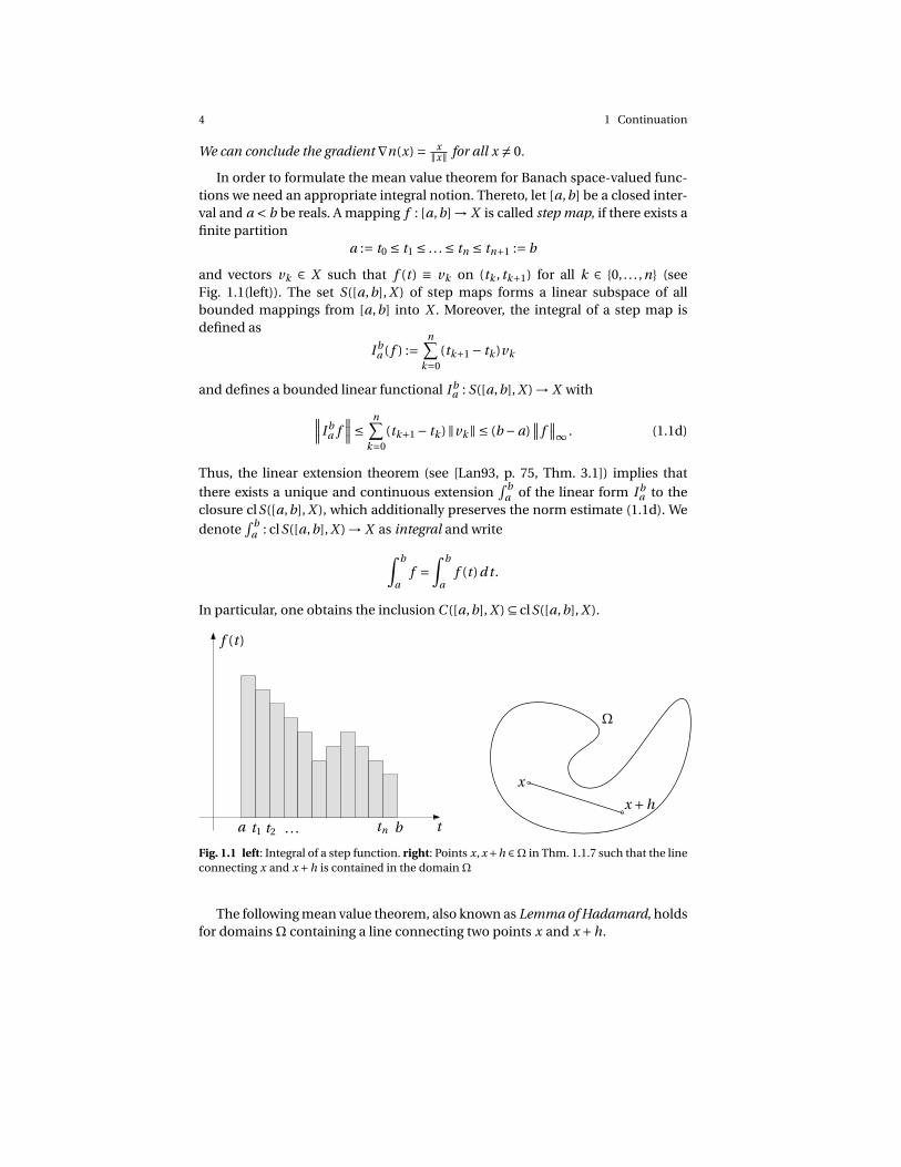
In the following, we describe a numerical method to compute smooth solutionpaths γ : U →Ω×Λ, U an open interval. If we differentiate the identity G(γ(s)) ≡ 0,one obtains

D1G(γ(s))γ1(s)+D2G(γ(s))γ2(s) ≡ 0 on U .

At a fold point (x0,λ0) = γ(s0) one has γ2(s0) = 0 and so γ1(s0) ∈ N (D1G(x0,λ0)).Consequently, D1G(x0,λ0) ∈ L(X , Z ) is not invertible and the continuationmethod described in Rem. 1.4.6 is not applicable.

2.3 Fold bifurcation 31

An alternative approach circumventing this problem is the pseudo-arclengthcontinuation. Thereto we retreat to the finite-dimensional situation X = Z = Rd .A solution path γ is called regular, if rk[D1G(γ(s)),D2G(γ(s))] = d for all s ∈U . Itis not difficult to see that this condition is satisfied, provided

• D1G(γ(s)) ∈GL(Rd ) or• dim N (D1G(γ(s))) = 1 and D2G(γ(s)) 6∈ R

(D1G(γ(s))

).

In particular, a regular solution path can contain fold points.

λ

x

γ(sk)

λk

xk

Pk

γ(sk+1)

γ

Fig. 2.3 Pseudo-arclength continuation

Now suppose that a point (x0,λ0) = γ(s0) on a regular solution path to (2.0a) isgiven. We are interested to find approximations (xk ,λk ) to the solution path γ atthe discrete points sk := s0+hk with a step size h 6= 0. The problem G(γ(sk )) = 0 isunderdetermined, since it consists of d equations for d+1 variables. We thereforecompute the norm-one tangent vector

γ(sk ) := 1‖γ(sk )‖

(γ1(sk )γ2(sk )

)and attach an additional scalar equation

⟨γ1(sk ), x −xk

⟩+ γ2(sk )(λ− λk ) = h,which describes the plane Pk ⊆ Rd ×R perpendicular to the tangent vector γ(sk )with distance h from (xk ,λk ) (see Fig. 2.3). Thus, in order to obtain (xk+1,λk+1)we solve H(x,λ) = 0 with the function

H(x,λ) :=(

G(x,λ)⟨γ1(sk ), x −xk

⟩+ γ2(sk )(λ−λk )−h

).


This can be done using a Newton method with initial value (xk ,λk ) + hγ(sk ).Hence, we obtain a predictor corrector method.

2.4 Bifurcation from simple eigenvalues

Now we deal with bifurcations from known solution branches and strengthen(2.0b) by assuming

G(x0,λ) ≡ 0 on Λ; (2.4a)

we do this w.l.o.g., since any nonconstant solution branch x∗(λ) ∈ Ω for (2.0a)can be transformed to the trivial branch. One replaces G with G(x + x∗(λ),λ)−G(x∗(λ),λ) having the trivial solution for all λ.

In this section we will prove the existence of another solution curve intersect-ing (x0,λ) : λ ∈Λ in the point (x0,λ0). We know such a situation from linear andnonlinear eigenvalue problems as introduced in Ex. 2.0.14 and Rem. 2.0.17.

Due to (2.4a) the function ϑ from Lemma 2.2.1 satisfies the identities

ϑ(0,λ) ≡ 0, D2ϑ(0,λ) ≡ 0 on Λ. (2.4b)

Also for the branching equation (2.2b) we get g (0,λ) ≡ 0 and consequently

D1g (0,λ0) = 0, D2g (0,λ) ≡ 0 on Λ. (2.4c)

Moreover, g allows the representation

g (v,λ) = vh(v,λ) for all v ∈V , λ ∈Λ0

with a C m−1-function h : V ×Λ0 → R satisfying the relation h(0,λ0) = 0. By themean value Thm. 1.1.7 it reads as

h(v,λ) =∫ 1

0D1g (t v,λ)d t .

The following bifurcation result is the celebrated Crandall-Rabinowitz theorem(see [CR71, Thm. 1.7] or [Zei93, p. 383, Thm. 8.A]).

Theorem 2.4.1 (bifurcation from simple eigenvalues). If Λ ⊆ R, m ≥ 2, therelations (2.3a), (2.4a) and the transversality condition

g11 :=µ(D1D2G(x0,λ0)x1) 6= 0 (2.4d)

hold, then (x0,λ0) is a bifurcation point of (2.0a). Precisely, there exist openconvex neighborhoods U ⊆R of 0, U1×U2 ⊆Ω×Λ of (x0,λ0) and a nontrivialC m−1-function γ= (γ1,γ2) : U →U1 ×U2 with

2.4 Bifurcation from simple eigenvalues 33

γ(U ) \ (x0,λ0) = (x,λ) ∈U1 ×U2 : G(x,λ) = 0 and x 6= x0 ,

where γ satisfies γ(0) = (x0,λ0) and γ1(0) = x1.

Remark 2.4.2. (1) The title of Thm. 2.4.1 can be motivated as follows: When deal-ing with nonlinear eigenvalue problems (2.0c), then the assumption (2.3a) meansdim N (DF (x0)−λ0 id) = 1, i.e. λ0 is a simple eigenvalue of DF (x0).

(2) The assumption (2.4a) of a constant solution branch can be avoided, ifone replaces the implicit mapping theorem in the subsequent proof by the Morselemma (cf. [Nir01, pp. 39ff, Chapt. 3]).

(3) In Exercise 2.4.6 we show the necessity of the transversality condition (2.4d).

Proof. Again we abbreviate T = D1G(x0,λ0). We intend to apply the implicit map-ping Thm. 1.4.3 to the scalar equation h(v,λ) = 0 with

h(v,λ) = [id−Q]∫ 1

0D1G (x0 + t v x1 +ϑ(t v,λ),λ) [x1 +D1ϑ(t v,λ)]d t .

In order to check the corresponding assumptions we deduce h(0,λ0) = 0 fromx1 ∈ N (T ) and Lemma 2.2.1. Moreover, it is

D2h(v,λ) = [id−Q]∫ 1

0D2

1G (x0 + t v x1 +ϑ(t v,λ),λ) [x1 +D1ϑ(t v,λ)]D2ϑ(t v,λ)d t

+[id−Q]∫ 1

0D1D2G (x0 + t v x1 +ϑ(t v,λ),λ) [x1 +D1ϑ(t v,λ)]d t

+[id−Q]∫ 1

0D1G (x0 + t v x1 +ϑ(t v,λ),λ)D1D2ϑ(t v,λ)d t

and thus by Lemma 2.2.1 and R(T ) = N (id−Q) it follows from

D2h(0,λ0) = [id−Q][D21G(x0,λ0)x1D2ϑ(0,λ0)+D1D2G(x0,λ0)x1

+T D1D2ϑ(0,λ0)](2.4b)= [id−Q]D1D2G(x0,λ0)x1 6= 0 (2.4e)

due to our assumption g11 6= 0. Consequently, Thm. 1.4.3 yields a C m−1-functionλ∗ : U → R such that h(v,λ∗(v)) ≡ 0 on U and λ∗(0) = λ0, g (v,λ∗(v)) ≡ 0 on U .Hence, the nonconstant solution branch is graph of the curve γ : U → Ω×Λ,γ(s) := (x0 + sx1 +ϑ(s,λ∗(s)),λ∗(s)), which fulfills (cf. Lemma 2.2.1 and (2.4c))

γ1(0) = x1 +D1ϑ(0,λ0)+D2ϑ(0,λ0)λ∗(0) = x1.

This yields our claim. ut

The precise shape of the curve γ(U ) from Thm. 2.4.3 can be obtained usingfurther information on the derivative of γ at 0.


Corollary 2.4.3 (abstract transcritical bifurcation). In case

g20 :=µ(D21G(x0,λ0)x2

1) 6= 0

one has γ2(0) =− g202g11

6= 0 and the following holds (see Fig. 2.4):

#x ∈U1 : G(x,λ) = 0 =

1, λ=λ0,

2, λ 6=λ0.

λλ

x x

λ0 λ0

x0x0

Fig. 2.4 Transcritical bifurcation

Proof. We compute the derivative

D1h(v,λ) =[id−Q]∫ 1

0D2

1G (x0 + t v x1 +ϑ(t v,λ),λ) ·

· [x0 + t x1 +D1ϑ(t v,λ)t ][x1 +D1ϑ(t v,λ)]d t

and thus using Lemma 2.2.1 it follows

D1h(0,λ0) = [id−Q]∫ 1

0D2

1G (x0 +ϑ(0,λ0),λ0) [t x1 +D1ϑ(0,λ0)t ][x1 +D1ϑ(0,λ0)]d t

= [id−Q]∫ 1

0tD2

1G (x0,λ0) x21 d t = 1

2[id−Q]D2

1G (x0,λ0) x21 .

On the other hand, differentiating the identity h(s,λ∗(s)) ≡ 0 implies

D1h(0,λ0)+D2h(0,λ0)λ∗(0) = 0

and thanks to (2.4e) it results γ2(0) = λ∗(0) =−D1h(0,λ0)D2h(0,λ0) =− g20

2g116= 0. This implies

our claim. ut

2.4 Bifurcation from simple eigenvalues 35

If the assumption g20 6= 0 is violated we get the following degenerate situation:

Corollary 2.4.4 (abstract pitchfork bifurcation). In case

µ(D21G(x0,λ0)x2

1) = 0, g30 :=µ(D31G(x0,λ0)x3

1) 6= 0

one has γ2(0) = 0, γ2(0) =− g303g11

and the following holds (see Fig. 2.5):

(a) If g30/g11 < 0, then #x ∈U1 : G(x,λ) = 0 =

1, λ≤λ0,

3, λ>λ0.

(b) If g30/g11 > 0, then #x ∈U1 : G(x,λ) = 0 =

1, λ≥λ0,

3, λ<λ0.

λλ

x x

λ0 λ0

x0x0

Fig. 2.5 Supercritical (left) and subcritical (right) pitchfork bifurcation

Remark 2.4.5. Again, the situation described in (a) is called supercritical bifurca-tion, whereas (b) is denoted as subcritical.

Proof. In case λ∗(0) = 0 the local shape of the curveγ is determined by the secondderivative λ∗(0). In order to compute it, we differentiate h(s,λ∗(s)) ≡ 0 on U twiceand obtain

d 2

d s2 h(s,λ∗(s))

∣∣∣∣s=0

= D21h(0,λ0)+D2h(0,λ0)λ∗(0) = 0,

since we assumed λ∗(0) = − g202g11

= 0. The term D2h(0,λ0) is known and

nonzero by (2.4e), thus λ∗(0) = −D21h(0,λ0)

D2h(0,λ0) . It remains to derive an expression for

D21h(0,λ0). For this purpose, using [id−Q]D1F (x0,λ0) = 0 we compute the higher

order derivatives

D21g (s,λ) =[id−Q]D2

1G(x0 + sx1 +ϑ(s,λ),λ)[x1 +D1ϑ(s,λ)]2


+ [id−Q]D1G(x0 + sx1 +ϑ(s,λ),λ)D21ϑ(s,λ),

D31g (0,λ0) =[id−Q]D3

1G(x0,λ0)x31

+3[id−Q]D21G(x0,λ0)x1D2

1ϑ(0,λ0).

Similarly, to the above this yields λ∗(0) =− g303g11

. ut

Exercises

Exercise 2.4.6. By means of the equation

G(x,λ) =(λx1 −x2 −x3

2λx2 +x3

1

)show that one cannot drop the transversality condition (2.4d) in Thm. 2.4.1.

Chapter 3

Application: Nonautonomous bifurcations

Throughout this chapter, let Λ ⊆ Y be an open and convex subset of a Banachspace Y . Given a continuous mapping f :Rd ×Λ→Rd , an autonomous differenceequation depending on the parameter λ ∈Λ is a recursion of the form

xk+1 = f (xk ,λ). (A)λ

The solutions to (A)λ can be represented using iterates of f (·,λ), namely

f 0(x,λ) := x, f k+1(x,λ) := f ( f k (x,λ),λ) for all k ∈N0, x ∈Rd , λ ∈Λ;

in case f (·,λ) is bijective, we additionally define f k (·,λ) := ( f −k (·,λ))−1 for inte-gers k < 0. Given an initial condition x0 = ξ ∈ Rd the unique forward solution to(A)λ has the representation

xk =φλ(k,ξ) := f k (ξ,λ) for all k ∈N0.

The resulting continuous mapping φλ :N0 ×Rd →Rd has the properties

(a) φλ(0, ·) = id,(b) φλ(k + l , ·) =φλ(k, ·)φλ(l , ·) for all k, l ∈N0, λ ∈Λ (semigroup property)

and φλ is called (discrete) semidynamical system or (discrete) semigroup. In casef (·,λ) is a homeomorphism, the above conditions hold for all k, l ∈ Z and onespeaks of a (discrete) dynamical system or a (discrete) group.

A fixed point of f (·,λ) is called equilibrium for φλ or (A)λ. A central questionin the theory of dynamical is the behavior of equilibria (or more general invariantsets) under varying parameters λ. If we suppose that for a particular parametervalue λ∗ there exists an equilibrium ξ∗ = f (ξ∗,λ∗) of (A)λ∗ , its robustness can bededuced from the implicit mapping Thm. 1.4.3. Indeed, provided f is sufficientlysmooth, we define F :Rd×Λ→Rd by F (x,λ) := f (x,λ)−x and obtain the relationsF (ξ∗,λ∗) = 0, D1F (ξ∗,λ∗) = D1 f (ξ∗,λ∗)− id. The condition 1 6∈ σ(D1 f (ξ∗,λ∗))guarantees that D1F (ξ∗,λ∗) is invertible. Thus, Thm. 1.4.3 implies that there ex-

37

38 3 Application: Nonautonomous bifurcations

ists a smooth mapping λ 7→ ξ(λ) satisfying ξ(λ∗) = ξ∗ and f (ξ(λ),λ) ≡ ξ(λ). Inparticular, each ξ(λ) is a locally unique fixed point of (A)λ.

The above situation becomes more involved (and interesting!), if we replaceour constant parameter λ by a sequence λk varying in (discrete) time k ∈Z. Thenthe difference equation (A)λ becomes nonautonomous and its solution is not asemidynamical system anymore.

3.1 Nonautonomous difference equations

A discrete interval I is the intersection of a real interval with the integers Z; weabbreviate I′ := k ∈ I : k +1 ∈ I and for κ ∈R also

Z+κ :=Z∩ [κ,∞), Z−

κ :=Z∩ (−∞,κ].

We restrict to finite-dimensional spaces Rd , whose norm is denoted by |·|.Given a sequence of mappings fk :Rd ×Λ→Rd , k ∈ I′, a parameter-dependent

nonautonomous difference equation is a recursion

xk+1 = fk (xk ,λ), (D)λ

Λ is denoted its parameter space and fk the right-hand side. For a fixed parameterλ ∈ Λ and a discrete interval J ⊆ I, a solution to (D)λ is a sequence φ = (φk )k∈Jsatisfying the solution identity

φk+1 ≡ fk (φk ,λ) on J′.

An entire solution is defined on the whole interval I. Given an initial time κ ∈ I andan initial value ξ ∈Rd one denotes the relation

xκ = ξ (3.1a)

as initial condition; the pair (D)λ, (3.1a) is an initial value problem. A solutionφ satisfying φκ = ξ is called solution of the initial value problem (D)λ, (3.1a). Aforward solution is a solution defined for times k ≥ κ and a backward solution isdefined dually. Note that forward solutions are determined uniquely and givenby the composition

ϕλ(k;κ,ξ) :=ξ, k = κ,

fk−1(·,λ) · · · fκ(ξ,λ), k > κ;

we denote ϕλ as general solution of (D)λ.

3.1 Nonautonomous difference equations 39

Proposition 3.1.1. Let λ ∈Λ. The general solution ϕλ : (k,κ,ξ) ∈ I× I×Rd :κ≤ k →Rd of (D)λ satisfies

(a) ϕλ(k;k, ·) = id,(b) ϕλ(k;κ, ·) = ϕλ(k; l ,ϕ(l ;κ, ·)) for all κ, l ,k ∈ I, κ ≤ l ≤ k (2-parameter

semigroup property).

If the right-hand sides fk (·,λ), k ∈ I′, in (D)λ are of class C m , m ∈ N0, thenalso ϕλ(k;κ, ·) :Rd →Rd , κ≤ k, is of class C m .

See Fig. 3.1 for an illustration of the 2-parameter semigroup property.

I

κ l k

ϕλ(l ;κ, ·)ϕλ(k; l , ·)

ϕλ(k;κ, ·)

Fig. 3.1 The 2-parameter semigroup property

Remark 3.1.2. (1) If (D)λ is an autonomous difference equation (A)λ with inducedsemigroup φλ, then one has the relation ϕλ(k;κ, ·) =φλ(k −κ, ·) for all κ≤ k.

(2) For C m-right-hand sides fk : Rd ×Λ→ Rd , k ∈ I′, also the general solution(ξ,λ) 7→ϕλ(k;κ,ξ), κ≤ k, is of class C m .

(3) Provided the mappings fk (·,λ) are bijective, the general solution ϕλ can beextended to the set I× I×Rd and the 2-parameter semigroup property holds for allk, l ,κ ∈ I, i.e. becomes a 2-parameter group property. A similar statement holdswith C m-diffeomorphisms.

Proof. See Exercise 3.1.6. ut

Differing from the territory of ordinary differential equations, backward solu-tions for initial value problems to difference equations need not to exist or to beunique. This is illustrated by the trivial

Example 3.1.3. Given an arbitrary ξ ∈R, every sequence (φk )k≥−1,

φk :=ξ, k =−1,

0, k ≥ 0


is a solution to the initial value problem xk+1 = 0, x0 = 0. On the other hand, theinitial value problem xk+1 = 0, x0 = 1 has no solution defined on a discrete intervalof the form Z+

−1.

Next we give two applications for infinite dimensional parameter spaces Λ.

Example 3.1.4 (parametric perturbation). Autonomous difference equations un-der parametric perturbations nicely fit in the above framework. Indeed, consider

xk+1 = g (xk , p)

with right-hand side g :Rd ×P →Rd , where P ⊆ Y is a nonempty open and convexset. Now the parameter p ∈ P is replaced by a sequence (pk )k∈I ∈ `∞(P ) and wearrive at a nonautonomous equation xk+1 = g (xk , pk ). For the parameter spaceΛ = `∞(P ) the mapping fk (x,λ) := g (x, pk ) with λ = (pk )k∈I satisfies Hyp. 1.3.1,provided one has g ∈ C m(Rd ×P,Rd ), the derivatives are uniformly continuous inp ∈ P and map bounded sets into bounded sets.

Example 3.1.5 (varying stepsizes). Let (τk )k∈Z be a strictly increasing sequenceof real numbers mimicking the time steps in a numerical scheme. A rudimentaryapproach to numerically approximate the solutions to ordinary differential equa-tions x = g (t , x) is the explicit Euler method

xk+1 = xk + (τk+1 −τk )g (τk , xk ); (3.1b)

this is a nonautonomous difference equation. In order to formulate (3.1b) in ourabstract set-up, we introduce the space `∞∆ := τ= (τk )k∈Z : (τk+1 −τk )k∈Z ∈ `∞ ofreal sequences. It becomes a Banach space w.r.t. the norm

|τ|∆ := max|τ0| , sup

k∈Z|τk+1 −τk |

.

If we define the evaluation and difference operators

evk : `∞∆ →R, evk τ := τk ,

∆k : `∞∆ →R, ∆kτ := τk+1 −τk ,

resp., then our explicit Euler-scheme (3.1b) can be written in the form (D)λ withright-hand side fk (x,τ) := x +∆kτg (evk τ, x) and parameter space Λ= `∞∆ .

We now retreat to an important class of difference equations, namely linearones. A difference equation is called linear, if it can be represented in the form

xk+1 = Ak xk +bk (3.1c)

with sequences Ak ∈Rd×d and bk ∈Rd for k ∈ I′. In case bk 6≡ 0 one denotes (3.1c)as linear-inhomogeneous and

xk+1 = Ak xk (3.1d)

3.1 Nonautonomous difference equations 41

is called linear-homogeneous. In order to represent the solutions to (3.1c) and(3.1d) we introduce the transition matrix Φ : (k, l ) ∈ I× I : l ≤ k →Rd×d ,

Φ(k, l ) :=

id, k = l ,

Ak−1 · · · Al , k > l .(3.1e)

For constant Ak ≡ A the representationΦ(k, l ) = Ak−l , l ≤ k, holds. The transitionmatrix Φ(·,κ) is a forward solution of the matrix initial value problem

Xk+1 = Ak Xk , Xκ = id

and the general solution to (3.1d) is given by

ϕ(k;κ,ξ) :=Φ(k,κ)ξ for all κ≤ k, ξ ∈Rd . (3.1f)

Equally evident is the linear 2-parameter semigroup property

Φ(k, l )Φ(l ,κ) =Φ(k,κ) for all κ≤ l ≤ k. (3.1g)

Under the assumption that all matrices Ak ∈ Rd×d , k ≤ I , are invertible, one canextend Φ to I× I by complementing (3.1e) with the definition

Φ(k, l ) := A−1k · · · A−1

l−1 for all k < l .

Then the relation (3.1f) holds for all k,κ ∈ I, (3.1g) holds for all k, l ,κ ∈ I and be-comes a linear 2-parameter group property, which implies

Φ(k, l ) =Φ(l ,k)−1 for all k, l ∈ I.

Moreover, it is possible to introduce the adjoint difference equation

xk+1 = (ATk+1)−1xk , (3.1h)

if Ak ∈Rd×d is invertible (and defined) for k ∈ I. Its transition operator reads as

Φ′(k, l ) =Φ(l +1,k +1)T for all k, l ∈ I′. (3.1i)

Exercises

Exercise 3.1.6. Prove Prop. 3.1.1.

Exercise 3.1.7 (variation of constants). Let Ak ∈Rd×d and bk ∈Rd for k ∈ I′. Find aformula for the general solution of the linear-inhomogeneous difference equation(3.1c). Under which assumption there exist backward solutions?

Exercise 3.1.8. Verify the relation (3.1i)!


3.2 Exponential dichotomies

A particular important class are the so-called hyperbolic matrices A ∈ Rd×d resp.hyperbolic difference equations

xk+1 = Axk , (3.2a)

which are characterized by the fact to have no eigenvalues on the unit circle in Caround 0. Their importance is due to the fact that also the perturbed matrix A+Bis hyperbolic, as long as B ∈ Rd×d has a small norm, as well as their prototypicaldynamical behavior:

Indeed, for a hyperbolic matrix A ∈Rd×d one has the spectral decomposition

σ(A) = λ1, . . . ,λn∪ λn+1, . . . ,λm

with integers 0 ≤ n ≤ m ≤ d , and∣∣λ j∣∣< 1 for all 1 ≤ j ≤ n,

∣∣λ j∣∣> 1 for all n < j ≤ m.

Moreover, if Eig j A ⊆ Rd denotes the generalized eigenspace1 corresponding tothe eigenvalue λ j , it is not difficult to deduce the dynamical characterization

V + :=ξ ∈Rd : lim

k→∞Akξ= 0

=

ξ ∈Rd : sup

k≥0

∣∣∣Akξ∣∣∣<∞

=⊕n

j=1 Eig j A,

V − :=ξ ∈Rd : lim

k→∞A−kξ= 0

=

ξ ∈Rd : sup

k≤0

∣∣∣Akξ∣∣∣<∞

=⊕m

j=n+1 Eig j A;

for simplicity we assume that A is invertible. For obvious reasons, V + is called thestable and V − the unstable subspace of (3.2a) (see Fig. 3.2); one has Rd =V −⊕V +.

=

<

Rd

V −

V +

Fig. 3.2 Hyperbolic spectral decomposition for A (left). Stable (green) subspace V + and unsta-ble (red) subspace V −

1 a generalized eigenspace is defined by the relation Eig j A :=⊕dk=1N (A−λ j id)k

3.2 Exponential dichotomies 43

Our next goal is to obtain a similar dynamical characterization for nonauto-nomous difference equations

xk+1 = Ak xk , (L)

where Ak ∈ Rd×d , k ∈ I, is assumed to be a sequence of invertible matrices; thelatter assumption is for the sake of a simple presentation only.

First, we need a counterpart to the invariant subspaces V −,V + ⊆ Rd from theautonomous case. For this it is convenient to introduce the notion of a nonauto-nomous set, which is a subset A ⊆ I×Rd . With this, the k-fiber, k ∈ I, is defined asA (k) :=

ξ ∈Rd : (k,ξ) ∈A.

Definition 3.2.1 (invariant projector). A sequence Pk ∈ Rd×d , k ∈ I, satisfy-ing Pk+1 Ak = Ak Pk for all k ∈ I′ is called an invariant projector of (L).

Corollary 3.2.2. If Pk ∈ Rd×d , k ∈ I, is an invariant projector of (L), thenΦ(k, l )Pl = PkΦ(k, l ) for all k, l ∈ I and the nonautonomous sets

V + :=

(κ,ξ) ∈ I×Rd : ξ ∈ R(Pκ)

, V − :=

(κ,ξ) ∈ I×Rd : ξ ∈ N (Pκ)

are invariant, i.e. V ±(k) =Φ(k,κ)V ±(κ) for all κ,k ∈Z.

Proof. The first claimed relation that Pk and Φ(k, l ) commute in the above senseeasily follows by mathematical induction. Given a pair (κ,ξ) ∈ V + we obtain

Φ(k,κ)ξ=Φ(k,κ)Pκξ= PkΦ(k,κ)ξ for all k ∈ I

and thus Φ(k,κ)ξ ∈ R(Pk ) = V +(k). The claim for V − follows analogously. ut

As demonstrated in Exercise 3.2.11 the k-dependent eigenvalues of Ak are ofno use in stability theory. However, the following notion is more fruitful:

Definition 3.2.3 (exponential dichotomy). A linear difference equation (L)is said to have an exponential dichotomy (ED for short) on I, if there existsan invariant projector Pk ∈Rd×d and reals 0 <α< 1 <β, K ≥ 1 so that

|Φ(k, l )Pl | ≤ Kαk−l for all l ≤ k,

|Φ(k, l )[id−Pl ]| ≤ Kβk−l for all k ≤ l .

Remark 3.2.4. (1) The dichotomy spectrum of (L) is the set


I

κ l k

Rd

Φ(l ,κ)

Φ(k, l )

R(Pκ)

R(Pk)

N (Pκ)

N (Pk)

Fig. 3.3 Geometric interpretation of an exponential dichotomy: The stable and unstable sub-space V + and V − from the autonomous situation (3.2a) are replaced by the respective fiberbundles V + and V −

Σ(A) := γ> 0 : xk+1 = γ−1 Ak xk does not have an ED

.

For autonomous equations (3.2a) one has Σ= |λ| : λ ∈σ(A).(2) In case (L) has an ED, then the nonautonomous sets V + and V − from

Cor. 3.2.2 satisfy the Whitney sum2

V +⊕V − = I×Rd

and are called stable resp. unstable vector bundle. This terminology is motivatedby the following

Proposition 3.2.5 (dynamical characterization of V ±). Suppose a linear dif-ference equation (L) has an ED on I.

(a) If I is unbounded above, then V + = (κ,ξ) ∈ I×Rd : supκ≤k |Φ(k,κ)ξ| <∞

.(b) If I is unbounded below, then V − =

(κ,ξ) ∈ I×Rd : supκ≥k |Φ(k,κ)ξ| <∞.

Proof. Let κ ∈ I.(a) We have to show two inclusions. Given ξ ∈ V +(κ) one has

|Φ(k,κ)ξ| = |Φ(k,κ)Pκξ| ≤ Kαk−κ |ξ| ≤ K |ξ| for all κ≤ k

and thus Φ(·,κ)ξ is bounded. Conversely, if the forward solution of (L) starting in(κ,ξ) ∈ I×Rd is bounded, there exists a real C > 0 such that

|Φ(k,κ)ξ| ≤C for all κ≤ k

and we obtain from Cor. 3.2.2 that

2 this means one has fiberwise V +(k)⊕V −(k) =Rd for all k ∈ I


|[id−Pκ]ξ| ≤ |Φ(κ,k)[id−Pk ]| |Φ(k,κ)ξ| ≤ Kβκ−k |Φ(k,κ)ξ| ≤C Kβκ−k

for all κ≤ k and in the limit k →∞ we obtain [id−Pκ]ξ= 0, i.e. ξ ∈ R(Pκ).(b) follows similarly. ut

Corollary 3.2.6.(a) If I is unbounded above, then (L) has exactly one solu-tion bounded on I in V −, namely the trivial one, and V + is uniquely de-termined.

(b) If I is unbounded below, then (L) has exactly one solution bounded on I inV +, namely the trivial one, and V − is uniquely determined.

(c) For I= Z the unique bounded entire solution of (L) is the trivial one andthe invariant projector Pk is uniquely determined.

Proof. Let κ ∈ I.(a) If φ is a bounded solution of (L) with φκ ∈ V −(κ), then Prop. 3.2.5 guaran-

tees φκ ∈ V +(κ)∩ V −(κ), which yields φκ = 0. Now suppose that (L) also has anED on I with an invariant projector Qk , k ∈ I, and stable vector bundle V +

Q . Sincethe dynamical characterization from Prop. 3.2.5 is independent of the projector,we get V + = V +

Q .(b) follows analogously.(c) The first assertion is an immediate consequence of (a) and (b). If (L) has

an ED on Z with another invariant projector Qk , we deduce from (a) and (b) thatV ± = V ±

Q , which means R(Pκ) = R(Qκ) and N (Pκ) = N (Qκ). This, however, impliesPκ =Qκ for all κ ∈Z. ut

Now we are in a position to treat inhomogeneous difference equation

xk+1 = Ak xk +bk , (3.2b)

where Ak ∈ Rd×d , k ∈ I′, is assumed to be a sequence of invertible matrices andbk ∈ I′. If Pk , k ∈ I, is an invariant projector for (L) we define the Green’s function

ΓP (k, l ) :=Φ(k, l )Pl , l ≤ k,

−Φ(k, l )[id−Pl ], k < l .

Proposition 3.2.7 (inhomogeneous perturbation on semiaxes). Supposethat (L) has an ED on I and κ ∈Z, b ∈ `∞.

(a) If I = Z+κ , then for every ξ ∈ Rd there exist a unique solution φ∗ ∈ `∞ to

(3.2b) satisfying Pκφ∗κ = Pκξ.

(b) If I = Z−κ , then for every ξ ∈ Rd there exist a unique solution φ∗ ∈ `∞ to

(3.2b) satisfying [id−Pκ]φ∗κ = [id−Pκ]ξ.


Proof. Letκ ∈Z and ξ ∈Rd be arbitrary. First, it is not difficult to verify the relation

ΓP (k +1, l ) = AkΓP (k, l )+δk,l−1 id. (3.2c)

(a) We formally define the sequence

φ∗k :=Φ(k,κ)Pκξ+

∞∑n=κ

ΓP (k,n +1)bn for all κ≤ k

and from the geometric series we obtain the estimate

∣∣φ∗k

∣∣ ≤ |Φ(k,κ)Pκ| |Pκξ|+∞∑

n=κ|ΓP (k,n +1)| |bn |

≤ Kαk−κ |Pκξ|+k−1∑n=κ

|Φ(k,n +1)Pn+1| |bn |+∞∑

n=k

|Φ(k,n +1)[id−Pn+1]| |bn |

≤ Kαk−κ |Pκξ|+Kk−1∑n=κ

αk−n−1 |bn |+K∞∑

n=kβk−n−1 |bn |

≤ K |Pκξ|+(

K

1−α + K

β−1

)supn≥κ

|bn | for all κ≤ k.

Hence, φ∗ is well-defined and in particular bounded. Moreover, we obtain thesolution identity

φ∗k+1 = Φ(k +1,κ)Pκξ+

∞∑n=κ

ΓP (k +1,n +1)bn

(3.2c)= AkΦ(k,κ)Pκξ+∞∑

n=κ

[AkΓP (k,n +1)+δk,n id

]bn = Akφ

∗k +bk for all κ≤ k,

as well as the relation

Pκφ∗κ = PκΦ(κ,κ)Pκξ+Pκ

∞∑n=κ

ΓP (κ,n +1)bn

= Pκξ−Pκ∞∑

n=κΦ(κ,n +1)[id−Pn+1]bn

= Pκξ−∞∑

n=κΦ(κ,n +1)Pn+1[id−Pn+1]bn = Pκξ.

Finally, letψ∗ be another bounded solution of (3.2b) satisfying Pκψ∗κ = Pκξ. Then

the difference δ :=φ∗−ψ∗ is a bounded solution of the linear homogenous equa-tion (L) satisfying Pκδκ = Pκ[φ∗

κ−ψ∗κ] = Pκξ−Pκξ= 0, which means δκ ∈ V −(κ).

We conclude from Cor. 3.2.6(a) that δ= 0, i.e. φ∗ =ψ∗.(b) Analogously using Cor. 3.2.6(b) one shows that

φ∗k :=Φ(k,κ)[id−Pκ]ξ+

κ−1∑n=−∞

ΓP (k,n +1)bn for all k ≤ κ


is the desired bounded backward solution. ut

Proposition 3.2.8 (inhomogeneous perturbation on Z). One has:

(a) If (L) has an ED on Z, then for every inhomogeneity b ∈ `∞ there exists aunique bounded solution to (3.2b).

(b) If supk∈Z |Ak | <∞, then also the converse to (a) holds true.

Proof. (a) We formally define the sequence

φ∗k :=

∑n∈Z

ΓP (k,n +1)bn for all k ∈Z (3.2d)

and using the geometric series we obtain the estimate

∣∣φk∣∣ ≤ k−1∑

n=−∞|ΓP (k,n +1)| |bn |+

∞∑n=k

|ΓP (k,n +1)| |bn |

=k−1∑

n=−∞|Φ(k,n +1)Pn+1| |bn |+

∞∑n=k

|Φ(k,n +1)[id−Pn+1]| |bn |

≤ Kk−1∑

n=−∞αk−n−1 |bn |+K

∞∑n=k

βk−n−1 |bn | ≤(

K

1−α + K

β−1

)supn∈Z

|bn |

for all k ∈Z. Therefore, φ∗ is well-defined and bounded. In addition, due to

φ∗k+1 =

∑n∈Z

ΓP (k +1,n +1)bn

(3.2c)=∑

n∈Z

[AkΓP (k,n +1)+δk,n id

]bn = Akφ

∗k +bk for all k ∈Z

it satisfies the solution identity for (3.2b). If ψ∗ denotes another bounded entiresolution to (3.2b), the difference δ :=ψ∗−φ∗ is a bounded entire solution of (L)and Cor. 3.2.6(c) implies δ= 0. Hence, ψ∗ is uniquely determined.

(b) is more involved and uses the closed graph theorem. A proof can be foundin [Hen81, p. 230, Thm. 7.6.5]. ut

Proposition 3.2.9 (`∞-roughness on Z). If (L) has an ED on I, then thereexists a δ> 0, such that also the perturbed difference equation

xk+1 = [Ak +Bk ] xk

has an ED on I, provided Bk ∈Rd×d , k ∈ I′, satisfies supk∈I′ |Bk | ≤ δ.


Proof. We only give a proof under the assumptions I=Z and supk∈Z |Ak | <∞ andrefer to [Pal88] for the general case.

We define the operator (L Aφ)k := φk+1 − Akφk for all k ∈ Z and easily see thatL A : `∞ → `∞ is linear and bounded. Moreover, thanks to Prop. 3.2.8(a) it is in-vertible. Referring to Exercise 1.1.10(a) the set GL(`∞) is open and consequentlyevery operator in a neighborhood of L A is invertible. In particular, there exists aδ> 0 such that also the inclusion L A+B ∈ L(`∞) holds, if ‖L A+B −L A‖ ≤ δ. Due toour assumption one actually has

‖L A+B −L A‖ = sup‖φ‖=1

∥∥(L A+B −L A)φ∥∥= sup

‖φ‖=1supk∈Z

∣∣Bkφk∣∣≤ sup

‖φ‖=1supk∈Z

|Bk |∥∥φ∥∥≤ δ

and the proof is established. ut

Exercises

Exercise 3.2.10. Suppose that P,Q ∈ L(X ) are bounded projections on a Banachspace X and show that

(a) id−P is also a projection and N (id−P ) = R(P ), R(id−P ) = N (P ),(b) N (P ) and R(P ) are closed subspaces of X with R(P )⊕N (P ) = X ,(c) R(P ) = R(Q) and N (P ) = N (Q) implies P =Q.

Exercise 3.2.11. Consider the nonautonomous difference equation (L) with the2-periodic coefficient matrix

Ak := 1

8

(0 9+7(−1)k

9−7(−1)k 0

)for all k ∈Z.

Show that (L) is unstable, i.e. has an unbounded solution, although the eigenval-ues of Ak have moduli less than 1.Hint: For ξ,η ∈R investigate the sequences

φk :=

(2−2kξ,2kη) for k even,(2kη,2−2kξ) for k odd.

Exercise 3.2.12. Assume A ∈ Rd×d has no eigenvalue of absolute value 1. Showthat the linear autonomous difference equation (3.2a) has an ED on Z. What canbe said about the invariant projectors Pk and the growth rates α?Hint: Transform A to Jordan canonical form!

Exercise 3.2.13. Suppose that (L) admits an exponential dichotomy on I with α

and invariant projector Pk . Show that also the adjoint equation (3.1h) has an ex-ponential dichotomy on J= k −1 ∈Z : k ∈ I with α and projector id−P T

k+1.

3.3 Entire solutions and invariant fiber bundles 49

3.3 Entire solutions and invariant fiber bundles

Now we return to a general nonlinear difference equation

xk+1 = fk (xk ,λ) (D)λ

with C m-smooth right-hand side fk : Rd ×Λ→ Rd , k ∈ I′, m ∈N, and general so-lution ϕλ. It allows the following abstract characterization

Theorem 3.3.1. Let λ ∈Λ. A sequence φ= (φk )k∈I solves the difference equa-tion (D)λ if and only if the relation

G(φ,λ) = 0

holds with G(φ,λ) = Sφ−N f (φ,λ), the shift operator (Sφ) := φk+1 and theNemytskii operator N f from Section 1.3.

Remark 3.3.2. Solutions defined on discrete intervals bounded above are bettercharacterized using the operator G(φ,λ)k =φk − fk−1(φk−1,λ).

Proof. By the solution identity 0 ≡ φk+1 − fk (φk ,λ) ≡ (Sφ)k −N f (φ,λ)k on I′ theproof is evident. ut

For a fixed parameter λ∗ ∈Λ we consider the so-called variational equation

xk+1 = D1 fk (φ∗k ,λ∗)xk (3.3a)

along a fixed reference sequence φ∗ = (φ∗k )k∈I. Typically, φ∗ is a solution to the

difference equation (D)λ∗ , like for instance an equilibrium or a periodic solution.Such a sequence is said to be hyperbolic, if (3.3a) has an ED on I. We define thedichotomy spectrum of φ∗ (see Rem. 3.2.4(1)) by

Σ(φ∗) :=Σ(A) with Ak := D1 fk (φ∗k ,λ∗)

and φ∗ is hyperbolic, precisely if 1 6∈Σ(φ∗).Now we have finally collected the preparations in order to deduce a nonauto-

nomous and discrete version of the Poincaré continuation lemma (see, for in-stance, [Ama95, p. 384, Thm. (25.2)]). It deals with the question, under whichconditions a bounded solutionφ∗ of the nonlinear difference equation (D)λ∗ per-sists, when the parameter λ is varied near λ∗ (see Fig. 3.4).

Theorem 3.3.3 (hyperbolic solutions on Z). Let λ∗ ∈ Λ, I = Z and supposefk satisfies Hyp. 1.3.1(a). If ` = `∞ and φ∗ ∈ ` is an entire solution of (D)λ∗such that


1 6∈Σ(φ∗),

then there exist ρ,ε> 0 and a C m-function φ : Bρ(λ∗) → Bε(φ∗) ⊆ ` with:

(a) φ(λ∗) =φ∗,(b) φ(λ) is the unique bounded entire solution of (D)λ in Bε(φ∗)×Bρ(λ∗),(c) φ(λ) is hyperbolic.

If also Hyp. 1.3.1(b) is satisfied, then the same holds with `= `0.

I

κ l k

Rd

R(Pκ)

R(Pk)

N (Pκ)

N (Pk)

φ∗κ

φ∗l

φ∗kφ(λ)κ

φ(λ)l

φ(λ)k

Fig. 3.4 Persistence of an entire solution φ∗ to (D)λ∗ as an entire solution φ(λ) to (D)λ undervariation of λ

Proof. (a) and (b) In case `= `∞ we use the implicit mapping Thm. 1.4.3 to solve

G(ψ,λ) = 0 for (ψ,λ) ∈ `∞×Λ.

Above all, note that G : `∞ ×Λ → `∞ is well-defined due to Prop. 1.3.5. Sinceφ∗ is a solution of (D)λ∗ we know from Thm. 3.3.1 that G(φ∗,λ∗) = 0 holds andwe have to show that the partial derivative D1G(φ∗,λ∗) ∈ L(`∞), which exists byProp. 1.3.5, is a toplinear isomorphism. We have the identity

D1G(φ∗,λ∗)φ= Sφ−N (1,0)f (φ∗,λ∗)φ. (3.3b)

Due to 1 6∈Σ(φ∗) and the resulting ED of (3.3a) onZwe deduce from Prop. 3.2.8(a)that D1G(φ∗,λ∗) is invertible and Thm. 1.4.3 yields the existence of a ρ > 0 and ofa unique C m-function φ : Bρ(λ∗) → `∞ such that G(φ(λ),λ) ≡ 0 on Bρ(λ∗).

(c) It remains to show the hyperbolicity of φ(λ). To establish this, note that thevariational difference equation xk+1 = D1 fk (φ(λ)k ,λ)xk can be written as

xk+1 = D1 fk (φ∗k ,λ∗)xk +

[D1 fk (φ(λ)k ,λ)−D1 fk (φ∗

k ,λ∗)]

xk . (3.3c)

Note that (3.3a) has an ED onZ. The continuity ofφ and D1 fk guarantees that forsufficiently small ρ > 0 one has

3.3 Entire solutions and invariant fiber bundles 51∣∣D1 fk (φ(λ)k ,λ)−D1 fk (φ∗k ,λ∗)

∣∣< δ for all k ∈Z, λ ∈ Bρ(λ∗),

with the δ > 0 from Prop. 3.2.9. Hence, this result implies that also (3.3c) admitsan ED on Z. Thus, φ(λ) is hyperbolic.

Now assume also Hyp. 1.3.1(b) and that φ∗ ∈ `0 holds. Then the above argu-ments including Prop. 3.2.8 remain true, when `∞ is replaced by `0. ut

Due to the differentiable dependence of the perturbed solution φ(λ) on theparameter λ ∈ Bρ(λ∗), one can approximate φ(λ) using a finite Taylor series inλ. Here, a phenomenon typical for nonautonomous equations occurs: Algebraicproblems in an autonomous setting become dynamical problems, i.e., instead ofsolving algebraic equations, one has to find bounded solutions of a nonautono-mous difference equation: As a result of Taylor’s Thm. 1.2.5 we can write

φ(λ) =φ∗+m∑

n=1

1

n!Dnφ(λ∗)(λ−λ∗)(n) +Rm(λ) (3.3d)

with coefficients Dnφ(λ∗) ∈ Ln(Y ,Rd ) and a remainder Rm satisfying the limitrelation limλ→0

Rm (λ)|λ|m = 0. For 1 ≤ n ≤ m we apply the higher order chain rule

(see [PR05, Lemma 4.1] for a reference in our notation) to the solution identityφ(λ)k+1 ≡ fk (φ(λ)k ,λ) on Bρ(λ∗) for all k ∈Z. This yields the relation

Dnφ(λ)k+1 y1 · . . . · yn = D1 fk (φ(λ)k ,λ)Dnφ(λ)k y1 · . . . · yn

+n∑

j=2

∑(N1,...,N j )∈P<

j (l )

D j fk (φ(λ)k ,λ)g #N1k (λ)yN1 · · ·g

#N j

k (λ)yN j

for all y1, . . . , yn ∈ Y , where we have abbreviated g #N1k (λ) := d #N1 (φ(λ)k ,λ)

dλ#N1. Setting

λ = λ∗ in this relation yields that the Taylor coefficients Dnφ(λ∗) ∈ Ln(Y ,`∞) ∼=`∞(Ln(Y ,Rd )) fulfill the linearly inhomogeneous difference equation

Xk+1 = D1 fk (φ∗k ,λ∗)Xk +Hn(k) (I )n

in Ln(Y ,Rd ), where the inhomogeneity Hn :Z→ Ln(Y ,Rd ) reads as

Hn(k)y1 · . . . · yn :=n∑

j=2

∑(N1,...,N j )∈P<

j (l )

D j fk (φ∗k ,λ∗)g #N1

k (λ∗)yN1 · · ·g#N j

k (λ∗)yN j ,

and in particular H1(k) = D2 fk (φ∗k ,λ∗). Using these preparations we can deduce

Corollary 3.3.4. The coefficients Dnφ(λ∗) :Z→ Ln(Y ,Rd ), 1 ≤ n ≤ m, in theTaylor expansion (3.3d) can be determined recursively from the Lyapunov-Perron sums


Dnφ(λ∗)k =∑l∈Z

ΓP (k, l +1)Hn(l ) for all 1 ≤ n ≤ m,

where ΓP is the Green’s function associated to (3.3a).

Proof. We prove the assertion by mathematical induction. For n = 1 the in-homogeneity H1 is bounded due to Hyp. 1.3.1(a). Since we want to approx-imate bounded solutions φ(λ) to equation (D)λ, it is reasonable to look forthe Taylor coefficient Dφ(λ∗) as bounded entire solution of (I )1. Arguing as inProp. 3.2.8, the ED of (3.3a) guarantees that the linear inhomogeneous equation(I )1 has a unique entire bounded solution which, thanks to (3.2d), is given by theLyapunov-Perron sum Dφ(λ∗)k =∑

l∈ZΓP (k, l +1)H1(l ).In the induction step n → n + 1 we see from the induction hypothesis that

the sequences Dφ(λ∗), . . . ,Dnφ(λ∗) are bounded, which implies that also Hn+1

is a bounded sequence. Therefore, due to the above argument, the linear equa-tions (I )n+1 has a unique bounded solution given by a Lyapunov-Perron sum asclaimed in our corollary. ut

The situation of Thm. 3.3.3 changes for one-sided time, where hyperbolic so-lutions are embedded in, and persist as, families of solutions parametrized overthe stable resp. unstable vector bundle associated with the linearization (3.3a).

Theorem 3.3.5 (hyperbolic solutions on semiaxes). Let λ∗ ∈ Λ, κ ∈ Z andsuppose fk satisfies Hyp. 1.3.1(a). If `= `∞ and φ∗ ∈ ` solves (D)λ∗ on Iwith

1 6∈Σ(φ∗) and associated invariant projector Pk , (3.3e)

then there exist δ,ρ > 0 such that:

(a) For I=Z+κ there is a unique ψ+ : Bρ(0,λ∗) ⊆ R(Pκ)×Λ→ Bδ(φ∗) ⊆ `∞,

(b) for I=Z−κ there is a unique ψ− : Bρ(0,λ∗) ⊆ N (Pκ)×Λ→ Bδ(φ∗) ⊆ `∞,

where ψ± are of class C m and for all (ξ,λ) ∈ Bρ(0,λ∗) one has:

(c) ψ±(0,λ∗) =φ∗,(d) ψ±(ξ,λ) is a hyperbolic solution of equation (D)λ.

If also Hyp. 1.3.1(b) is satisfied, then the same holds with `= `0.

Proof. We present the proof only for `∞ and set L := D1G(φ∗,λ∗).Let I=Z+

κ . Since (3.3a) admits an ED on Z+κ we deduce from Prop. 3.2.7(a) that

the derivative D1G(φ∗,λ∗) ∈ L(`∞) is onto. Moreover, thanks to Prop. 3.2.5(a) ithas the finite-dimensional kernel

N (D1G(φ∗,λ∗)) = Φ(·,κ)ξ : ξ ∈ V +(κ)

∼= R(Pκ),

3.3 Entire solutions and invariant fiber bundles 53

which is complemented, i.e., `∞ = N (L)⊕Z with a closed subspace Z ⊆ `∞. Thusthe claims (a) and (c) follow from the surjective implicit mapping Thm. 1.4.10applied to G(φ∗,λ∗) = 0. The hyperbolicity of ψ+(ξ,λ) follows as in Thm. 3.3.3(c)using Prop. 3.2.9, which establishes the assertion (d).

The case I=Z−κ follows dually using Prop. 3.2.7(b) and 3.2.5(b). ut

We close this section with a short and elegant proof of a nonautonomous sta-ble/unstable manifold theorem, which we denote as invariant fiber bundles. Forthis, let I be a discrete unbounded interval and φ∗ = (φ∗

k )k∈I be a bounded solu-tion of (D)λ∗ , λ∗ ∈Λ. Then the respective nonautonomous sets defined as

S ±λ

:=

(κ,ξ) ∈ I×Rd : ϕλ(k;κ,ξ)−φ∗k −−−−−→

k→±∞0

are denoted as stable resp. unstable set of φ∗. Locally they are given as graphsof C m-mappings over the stable resp. unstable vector bundle V + and V − of theassociated variational equation (3.3a):

Corollary 3.3.6 (invariant fiber bundles). If φ∗ ∈ `∞ is a solution of (D)λ∗on I satisfying (3.3e), then there exist ε,ρ > 0 such that:

(a) In case I is unbounded above, for every κ ∈ I there is a unique C m-functions+κ : Bρ(0,λ∗) ⊆ R(Pκ)×Λ→ N (Pκ) so that the fibers of S +

λfulfill

S +λ (κ)∩Bε(φ∗

κ) =φ∗κ+ξ+ s+κ (ξ,λ) ∈Rd : ξ ∈ Bρ(0) ⊆ R(Pκ)

,

(b) in case I is unbounded below, for every κ ∈ I there is a unique C m-functions−κ : Bρ(0,λ∗) ⊆ N (Pκ)×Λ→ R(Pκ) so that the fibers of S −

λfulfill

S −λ (κ)∩Bε(φ∗

κ) =φ∗κ+ξ+ s+κ (ξ,λ) ∈Rd : ξ ∈ Bρ(0) ⊆ N (Pκ)

for all λ ∈ Bρ(λ∗) (see Fig. 3.5).

Proof. We consider the difference equation of perturbed motion

xk+1 = fk (xk +φ∗k ,λ)− fk (φ∗

k ,λ) (3.3f)

which admits the trivial solution on I for all λ ∈Λ. Moreover, it satisfies Hyp. 1.3.1and we choose κ ∈ I.

(a) For Z+κ the above Thm. 3.3.5(a) applies to (3.3f). This implies

S +λ (κ)∩Bε(φ∗

κ) =φ∗κ+ψ+(ξ,λ)κ ∈Rd : ξ ∈ Bρ(0) ⊆ R(Pκ)


I

κ l k

Rd

R(Pκ)

R(Pk)

N (Pκ)N (Pk)

φ∗κ

φ∗l

φ∗k

S −λ

(k)

S +λ

(k)

Fig. 3.5 Perturbed stable invariant fiber bundle S +λ

and unstable invariant fiber bundle S −λ

asgraphs over the stable resp. unstable vector bundle V + and V −

and the surjective implicit mapping Thm. 1.4.10 yields that solutions of (3.3f) de-caying to 0 in forward time, start inψ(ξ,λ)κ = ξ+φ(ξ,λ)κ with a C m-functionφ(·)κhaving values in N (Pκ). Then the assertion follows with s+κ (ξ,λ) :=φ(ξ,λ)κ.

(b) follows along the same lines with Thm. 3.3.5(b). ut

Exercises

Exercise 3.3.7. Let α,β,λ ∈ R with |α| 6= 1 and |β| < 1. Determine all entirebounded solutions of the autonomous difference equation

xk+1 =αxk +λ.

Do these entire bounded solutions also solve the nonautonomous equation

xk+1 =αxk +λβ|k|?

Can you illustrate Thm. 3.3.3 using the present example for an appropriate valueof λ∗ and explicitly compute the sequence φ(λ)?

3.4 Bifurcation of entire solutions

We assume for a parameter λ=λ∗ ∈Λ the nonautonomous difference equation

xk+1 = fk (xk ,λ) (D)λ

in Rd has a bounded entire reference solution φ∗ = φ(λ∗). We say that (D)λ un-dergoes a bifurcation at λ = λ∗ along φ∗, or φ∗ bifurcates at λ∗, if there exists aconvergent sequence of parameters (λn)n∈N in Λ with limit λ∗ so that (D)λn has

3.4 Bifurcation of entire solutions 55

two distinct bounded entire solutions φ1(λn),φ2(λn) satisfying

limn→∞φ

1(λn) = limn→∞φ

2(λn) =φ∗.

Given a parameter space Λ ⊆ R, one speaks of a subcritical or a supercritical bi-furcation, if the sequence (λn)n∈N can be chosen according toλn <λ∗ orλn >λ∗,respectively. In other words, the pair (φ∗,λ∗) is a bifurcation or branching pointof the abstract nonlinear equation

G(φ,λ) = 0 (3.4a)

in `∞ from Thm. 3.3.1 in the sense of Def. 2.0.13. From Prop. 2.0.15 we obtain

Proposition 3.4.1. Let λ∗ ∈ Λ and suppose Hyp. 1.3.1(a) holds. If an entiresolution φ∗ ∈ `∞ of (D)λ∗ bifurcates at λ∗, then φ∗ is nonhyperbolic.

Proof. We suppose 1 6∈Σ(φ∗) and our Thm. 3.3.3 guarantees that neighborhoodsΛ0 ⊆ Λ for λ∗, U ⊆ `∞ for φ∗ exist, so that (D)λ has a unique entire solutionφ(λ) ∈U for λ ∈Λ0. Consequently, φ∗ cannot bifurcate at λ∗. ut

Hence, in order to obtain bifurcation results for entire solutions, we have to as-sume weaker concepts than an exponential dichotomy on the whole integer axis.One possibility, namely dichotomies on both semiaxes, will be discussed now.

Hypothesis 3.4.1. Let n,r ∈ N, κ ∈ Z, λ∗ ∈ Λ be given, suppose (D)λ∗ admits anentire solution φ∗ ∈ `∞ whose variational equation (3.3a) admits an ED both onZ+κ and Z−

κ with respective projectors P+k and P−

k satisfying

R(P+κ )∩N (P−

κ ) = spanξ1, . . . ,ξn , (R(P+κ )+N (P−

κ ))⊥ = spanξ′1, . . . ,ξ′r

and linearly independent vectors ξ1, . . . ,ξn ∈ Rd , resp. ξ′1, . . . ,ξ′r ∈ Rd . Moreover,we choose η1, . . . ,ηr ∈Rd , resp. η′1, . . . ,η′n ∈Rd such that⟨

η′i ,ξ j⟩= δi , j for 1 ≤ i , j ≤ n,

⟨ξ′i ,η j

⟩= δi , j for 1 ≤ i , j ≤ r. (3.4b)

Remark 3.4.2. (1) We have orthogonality⟨ξ′i ,ξ j

⟩= 0 for 1 ≤ i ≤ n, 1 ≤ j ≤ r .(2) In order to satisfy Hyp. 3.4.1 it is necessary to require d > 1 and the conditions

n,r ∈ N demand P+κ 6= id, P−

κ 6= 0 and P+κ 6= 0, P−

κ 6= id. The existence of an ED onZ+κ with nontrivial unstable vector bundle yields the solution φ∗ is unstable.

Next we apply the Fredholm theory from Sect. 2.1 to the difference operator

L : `→ `, (Lφ)k :=φk+1 −D1 fk (φ∗k ,λ∗)φk , (3.4c)

where ` denotes either `∞ or `0. Due to the boundedness of φ∗ and Hyp. 1.3.1(a)the operator L is well-defined and bounded. So is the dual operator


(L′ψ)k :=ψk+1 −D1 fk+1(φ∗k+1,λ∗)−Tψk .

Lemma 3.4.3. If Hyp. 1.3.1(a), 3.4.1 hold, then the linear operator L : ` → ` isFredholm of index n − r and

N (L) = spanΦλ∗ (·,κ)ξ1, . . . ,Φλ∗ (·,κ)ξn ,

N (L′) = spanΦλ∗ (κ, ·+1)T ξ′1, . . . ,Φλ∗ (κ, ·+1)T ξ′r

, (3.4d)

where Φλ∗ (·,κ)ξi , 1 ≤ i ≤ n, resp. Φλ∗ (κ, ·+1)T ξ′j , 1 ≤ j ≤ r , are linearly indepen-

dent.

Proof. (I) Let ξ ∈ R(P+κ )∩N (P−

κ ) and Prop. 3.2.5 ensures Φλ∗ (·,κ)ξ ∈ N (L). More-over, the mapping ξ 7→Φ(·,κ)ξ is an isomorphism and thus

dim N (L) = dimR(P+κ )∩N (P−

κ ) = n.

(II) Thanks to Exercise 3.2.13 we know that also the adjoint equation (3.1h)admits EDs onZ−

κ−1,Z+κ−1 with respective projectors (id−P−

k+1)T and (id−P+k+1)T .

An application of Prop. 3.2.5 yields that η 7→Φ′λ∗ (·,κ−1)η is an isomorphism from

R(id−P+κ )T ∩N (id−P−

κ )T = R(P+κ )⊥∩N (P−

κ )⊥ = (R(P+κ )+N (P−

κ ))⊥

onto N (L′). This guarantees the relation (see [Zei93, p. 366, Prop. 8.14(4)])

codimR(L) = dim N (L′) = codimR(P+κ )+N (P−

κ ) = r

and consequently L ∈ L(`) is Fredholm with index n − r . ut

Lemma 3.4.4. If Hyp. 1.3.1(a), 3.4.1 hold, then the mappings P,Q ∈ L(`),

P x :=n∑

i=1

⟨η′i , xκ

⟩Φλ∗ (·,κ)ξi , Qx := x −Eκ

r∑i=1

∑j∈Z

⟨Φλ∗ (κ, j +1)T ξ′i , x j

⟩ηi

are bounded projections onto N (L) and R(L), resp., where Eκ :Rd → ` reads as

(Eκξ)k := δk,κξ.

Proof. Following the procedure given in Sect. 2.1 we introduce a bilinear form

⟨·, ·⟩ : `β×`→R,⟨φ′,ψ

⟩:=

∑j∈Z

⟨φ′

j ,ψ j

⟩, (3.4e)

where `β is the β-dual of `, i.e. the set of all sequences φ′ = (φ′j ) j∈Z in Rd such

that⟨φ′, ·⟩ defines a continuous linear form on the sequence space `. Now, from

Lemma 3.4.3 we know that the linearly independent vectors φi :=Φλ∗ (·,κ)ξi in `span the kernel N (L). Thus, if we define sequences ψ′

i ∈ `β by ψ′i := δ·,κη′i our as-

sumption (3.4b) implies⟨ψ′

i ,φ j⟩= ⟨

ψ′i ,κ,φ j

κ

⟩= ⟨

η′i ,ξ j⟩= δi , j and

ψ′

i ,φ j

forms


a biorthogonal system. Then

P x :=n∑

i=1

⟨ψ′

i , x⟩φi =

n∑i=1

⟨η′i , xκ

⟩φi =

n∑i=1

⟨η′i , xκ

⟩Φλ∗ (·,κ)ξi

is a projection P ∈ L(`) onto N (L). Defining sequences φ′i ∈ `β, ψi ∈ ` by

φ′i :=Φλ∗ (κ, ·)T ξ′i , ψi := Eκηi for all 1 ≤ i ≤ r

we obtain from (3.4b) that⟨φ′

i ,ψ j⟩ = ⟨

ξ′i ,η j⟩ = δi , j ; thus, also

φ′

i ,ψ j

forms abiorthogonal system. In addition, we define a projection id−Q ∈ L(`) given by

(id−Q)y :=r∑

i=1

⟨φ′

i , y⟩ψi = Eκ

r∑i=1

∑j∈Z

⟨Φλ∗ (κ, j +1)T ξ′i , y j

⟩ηi ,

whose complementary projection Q maps onto R(L). ut

At this point it is possible to obtain the explicit form of the branching equation(2.2b) in our particular situation. However, since there is no need to do so forour further applications, we leave this task to the interested reader. We ratherintroduce certain functionals:

Lemma 3.4.5. If Hyp. 1.3.1(a), 3.4.1 hold, then the linear functionals

µi : `→R, µi (φ) :=∑j∈Z

⟨Φλ∗ (κ, j +1)T ξ′i ,φ j

⟩for all 1 ≤ i ≤ r

are continuous with∣∣µi

∣∣≤ K 1+α1−α

∣∣ξ′i ∣∣ and one has R(L) =⋂ri=1 N (µi ).

Proof. The vectors ξ′i ∈Rd from Hyp. 3.4.1 satisfy

ξ′i ∈ (R(P−κ )+N (P+

κ ))⊥ = R((id−P+κ )T )∩N (id−P−

κ )T )

and thus, using the assumed dichotomy estimates, we estimate µi (φ) as follows

∣∣µi (φ)∣∣≤ κ−1∑

j=−∞

∣∣⟨Φλ∗ (κ, j +1)T P−κ ξ

′i ,φ j

⟩∣∣+ ∞∑j=κ

∣∣⟨Φλ∗ (κ, j +1)T (id−P+κ )ξ′i ,φ j

⟩∣∣≤

κ−1∑j=−∞

∣∣∣Φλ∗ (κ, j +1)P−j+1

∣∣∣ ∣∣ξ′i ∣∣ ∣∣φ j∣∣+ ∞∑

j=κ

∣∣∣Φλ∗ (κ, j +1)(id−P+j+1)

∣∣∣ ∣∣ξ′i ∣∣ ∣∣φ j∣∣

≤ K∣∣ξ′i ∣∣∥∥φ∥∥(

κ−1∑j=−∞

ακ− j−1 +∞∑

j=κα j+1−κ

)for all 1 ≤ i ≤ r.

This implies the given bound for∣∣µi

∣∣. From Lemma 3.4.3 we get that the operatorL is Fredholm and [Zei93, p. 366, Prop. 8.14(2)] guarantees the equivalences

φ ∈ R(L) ⇔ φ ∈ N (L′)⊥ ⇔ ⟨ψ′,φ

⟩= 0 for all ψ′ ∈ N (L′)


(3.4d)⇔ ⟨Φλ∗ (κ, ·+1)T ξ′i ,φ

⟩= 0 for all 1 ≤ i ≤ r

⇔∑j∈Z

⟨Φλ∗ (κ, j +1)T ξ′i ,φ j

⟩= 0 for all 1 ≤ i ≤ r

⇔ µi (φ) = 0 for all 1 ≤ i ≤ r ⇔φ ∈r⋂

i=1N (µi ),

which leads to our assertion. ut

We sometimes retreat to the following simplification:

Hypothesis 3.4.2. Let fk (0,λ) ≡ 0 on Z×Λ.

Remark 3.4.6. Obviously, Hyp. 3.4.2 implies Hyp. 1.3.1(b) and since the trivial so-lution branch consists of sequences in `0, it is reasonable to search in `0 (insteadof `∞) for bifurcating solutions of (D)λ, i.e. we are interested in the branching ofsolutions heteroclinic to 0.

At this point we apply the abstract bifurcation results of Sect. 2.3 to (3.4a). Wefirst address the simple situation of linear difference equations:

Example 3.4.7 (linear homogeneous equation). Suppose that α ∈ (−1,1) and γ

are fixed nonzero reals. We consider the linear homogeneous difference equation

xk+1 = fk (xk ,λ) :=(

bk 0λγ ck

)xk (3.4f)

depending on a parameter λ ∈Rwith asymptotically constant sequences

bk :=α−1, k < 0,

α, k ≥ 0,ck :=

α, k < 0,

α−1, k ≥ 0.(3.4g)

It is easily seen that equation (3.4f) fulfills Hyp. 1.3.1, 3.4.2 and we set κ= 0,φ∗ = 0,λ∗ = 0. Furthermore, we deduce that also Hyp. 3.4.1 holds with n = r = 1 and theinvariant projectors P+

k ≡ (1 00 0

)and P−

k ≡ (0 00 1

). This yields

R(P+0 )∩N (P−

0 ) =R(10

), R(P+

0 )+N (P−0 ) =R

(10

)and we can choose the vectors ξ1 =

(10

), ξ′1 =

(01

). After these observations the linear

functional µ1 : `0 →R from Lemma 3.4.5 computes as

µ1(φ) =∑j∈Z

⟨ξ′1Φ0(0, j +1)T ,φ j

⟩=

−2∑j=−∞

⟨ξ′1Φ0(0, j +1)T ,φ j

⟩+⟨ξ′1,φ−1

⟩+ ∞∑j=0

⟨ξ′1Φ0(0, j +1)T ,φ j

⟩=

∑j∈Z

α| j+1|φ2j , (3.4h)


where φ= (φ1,φ2) ∈ `0.In order to illustrate a possible bifurcation scenario, we exploit the simple tri-

angular structure of (3.4f) and compute its general solutionϕλ(·;0,η) for arbitraryinitial values η ∈R2. For the first component ϕ1

λwe obtain that

ϕ1λ(k;0,η) =α|k|η1 for all k ∈Z, η ∈R2 (3.4i)

and thus ϕ1λ

(·;0,η) ∈ `0. The second component can be tackled using the variationof constants formula (cf. Exercise 3.1.7). Before doing this, for later use we establishthe following elementary summation formulas

k−1∑n=0

αmn

αk−n−1=αα

mk −α−k

αm+1 −1for all m ∈N0, k ∈N,

−1∑n=k

αk−n−1

αmn =αm α−mk −αk

αm+1 −1for all m ∈N0, k < 0.

(3.4j)

Then the second component of ϕλ reads as

ϕ2λ(k;0,η) =α−|k|η2 +λγ

∑k−1n=0

1αk−n−1α

nη1, k ≥ 0,

−∑−1n=k α

k−n−1α−nη1, k < 0

and together with (3.4j) we arrive at the asymptotic relation

ϕ2λ(k;0,η) =

α−k

(η2 − λαγ

α2−1η1

)+o(1), k →∞,

αk(η2 + λαγ

α2−1η1

)+o(1), k →−∞.

Consequently, forλ 6= 0 the inclusionϕλ(·;0,η) ∈ `0 holds if and only if η2 = λαγ

α2−1η1

and η2 =− λαγ

α2−1η1, i.e. η= (0,0). In conclusion, 0 is the unique homoclinic solution

to (3.4f) for λ 6= 0, while in case λ= 0 the trivial solution φ∗ = 0 is embedded into awhole 1-parameter family of homoclinic solutions sΦ0(·,0)ξ1 (see Fig. 3.6 (left)).

Λ

λ < λ∗

λ = λ∗

λ > λ∗

R2

R2

R2

Λ

λ < λ∗

λ = λ∗

λ > λ∗

R2

R2

R2

Fig. 3.6 Left: Initial values η ∈ R2 yielding a homoclinic solution ϕλ(·;0,η) of (3.4f) for differentparameter values λ.Right: Initial values η ∈R2 yielding a bounded solutionϕλ(·;0,η) of (3.4k) for different parametervalues λ


Remark 3.4.8 (bifurcation diagrams). Do not understand Figs. 3.6, 3.7 and 3.8as bifurcation diagrams, i.e. subset of Λ×` indicating bounded solutions to (D)λ.Indeed, they are subsets of Λ×R2 indicating initial values η yielding bounded orhomoclinic solutions ϕλ(·;0,η) to the respective difference equations treated in theExamples 3.4.7, 3.4.10, 3.4.14 and 3.4.16.

Specific results for nonlinear problems can be obtained for index 0 Fredholmoperators with 1-dimensional kernel. For our first result we need not to impose atrivial solution branch as in Hyp. 3.4.2.

Theorem 3.4.9 (fold bifurcation). Let Λ⊆R and suppose that Hyp. 1.3.1(a),3.4.1 hold with n = r = 1. If `= `∞ and

g01 :=∑j∈Z

⟨Φλ∗ (κ, j +1)T ξ′1,D2 f j (φ∗

j ,λ∗)⟩6= 0,

then there exists a ρ > 0, open convex neighborhoods U ⊆ `∞ of φ∗, Λ0 ⊆Λ

of λ∗ and C m-functions φ : (−ρ,ρ) →U , λ : (−ρ,ρ) →Λ0 such that

(a) φ(0) =φ∗, λ(0) =λ∗ and φ(0) =Φλ∗ (·,κ)ξ1, λ(0) = 0,(b) each φ(s) is an entire solution of (D)λ(s) in `.

Moreover, in case m ≥ 2 and under the additional assumption

g20 :=∑j∈Z

⟨Φλ∗ (κ, j +1)T ξ′1,D2

1 f j (φ∗j ,λ∗)[Φλ∗ ( j ,κ)ξ1]2

⟩6= 0,

the solution φ∗ ∈ ` of (D)λ∗ bifurcates at λ∗, one has λ(0) = − g20g01

and thefollowing holds locally in U ×Λ0:

(c) Subcritical case: If g20/g01 > 0, then (D)λ has no entire solution in `∞

for λ > λ∗, φ∗ is the unique entire solution of (D)λ∗ in `∞ and (D)λ hasexactly two entire bounded solutions for λ<λ∗; they are in `.

(d) Supercritical case: If g20/g01 < 0, then (D)λ has no entire solution in `∞

for λ < λ∗, φ∗ is the unique entire solution of (D)λ∗ in `∞ and (D)λ hasexactly two entire bounded solutions for λ>λ∗; they are in `.

If Hyp. 1.3.1 to 3.4.1 are satisfied, then the same holds with `= `0.

Proof. Our strategy is to apply the abstract Thm. 2.3.1 with x1 = Φλ∗ (·,κ)ξ1 to(3.4a). By Thm. 3.3.1(a) the mapping G : `∞ ×Λ → `∞ is of class C m and wehave G(φ∗,λ∗) = 0. With the functional µ = µ1 from Lemma 3.4.5 we calculate−µ(D2G(φ∗,λ∗)) = g01 and Thm. 2.3.1 guarantees a solution curve γ= (γ1,γ2) for(3.4a); we define φ := γ1 and λ := γ2. For at least C 2-smooth right-hand sides fk

we also get −µ(D21G(x0,λ0)x2

1) = g20 and the claim follows in case `= `∞. Yet, un-der additionally Hyp. 1.3.1(b) the above arguments also apply to G : `0 ×Λ→ `0

and the bounded bifurcating solutions are actually in `0. ut


Example 3.4.10 (inhomogeneous equations). Let α ∈ (−1,1) and γ,δ be fixednonzero reals. We initially consider the linear inhomogeneous difference equation

xk+1 = fk (xk ,λ) :=(bk 00 ck

)xk +λ

(0γ

)(3.4k)

depending on a bifurcation parameterλ ∈R and sequences bk ,ck defined in (3.4g).As in the previous Ex. 3.4.7 we see that (3.4k) fulfills Hyp. 1.3.1(a) and 3.4.1 withκ = 0, φ∗ = 0, λ∗ = 0 and ξ1 = (

10

). Moreover, due to D2 f j (0,0) ≡ ( 0

γ

)one obtains

from (3.4h) that

g01 =∑j∈Z

α| j+1|γ= γ1+α1−α 6= 0.

A detailed picture follows using the general solution ϕλ(·;0,η) of (3.4k). Its firstcomponentϕ1

λis given by (3.4i), while the second component follows from the vari-

ation of constants formula (cf. Exercise 3.1.7). Using the relations (3.4j) one deduces

ϕ2λ(k;0,η) =

α−k

(η2 − λαγ

α−1

)+O(1), k →∞,

αk(η2 + λγ

α−1

)+O(1), k →−∞,

and so the inclusion ϕλ(·;0,η) ∈ `∞ holds if and only if both conditions η2 = λαγα−1

and η2 =− λγα−1 are satisfied. This, however, is not possible unless λ= 0. In conclu-

sion, there exists no bounded entire solution of (3.4k) for λ 6= 0, while there is a1-parameter family of bounded solutions in case λ = 0. In the terminology intro-duced in Thm. 3.4.9 this means φ(s) = sΦ0(·,0)ξ1 = s

(α|·|0

)and λ(s) ≡ 0 for all s ∈R.

Also the zero solution to (3.4k) bifurcates at λ= 0.It is understood that the linear equation (3.4k) does not fulfill the condition

g20 6= 0 yielding a fold. In fact, the situation becomes more interesting, if we con-sider the following nonlinear perturbation of (3.4k) defined as

xk+1 = fk (xk ,λ) :=(bk 00 ck

)xk +δ

(0

(x1k )2

)+λ

(0γ

)(3.4l)

with xk = (x1k , x2

k ). Our hypotheses Hyp. 1.3.1(a) and 3.4.1 are fulfilled with the

data given above. Moreover, the relation D21 f j (0,0)ζ2 = ( 0

2δζ21

)for all j ∈ Z, ζ ∈ R2

and (3.4h) ensure

g20 = 2δα+α2

1−α3 6= 0.

Hence, Thm. 3.4.9 shows that the zero solution to (3.4l) has a fold bifurcation atλ= 0. Due to g20

g01= δ

γ2α

1+α+α2 it is subcritical forαδγ > 0 and supercritical forαδ

γ < 0.We are able to verify this statement explicitly using the general solution

ϕλ(·;0,η) to (3.4l). Its first component ϕ1λ

has been computed in (3.4i), while thevariation of constants formula (cf. Exercise 3.1.7) and (3.4j) can be used to deducethe asymptotic representation


ϕ2λ(k;0,η) =

α−k

(η2 − δα

α3−1η2

1 −λαγα−1

)+O(1), k →∞,

αk(η2 + δα2

α3−1η2

1 +λγα−1

)+O(1), k →−∞.

Therefore, the sequence ϕλ(·;0,η) is bounded if and only if η2 = δαα3−1

η21 +

λαγα−1 and

η2 = − δα2

α3−1η2

1 −λγα−1 holds, i.e. η2

1 = −α2+α+1α

γδλ, η2 = γλ. From the first relation

we see that there exist two bounded solutions, if αδγλ< 0, the trivial solution is the

unique bounded solution for λ= 0 and there are no bounded solutions for αδγλ>

0. This perfectly corresponds to the above fold bifurcation pattern deduced fromThm. 3.4.9 and we refer to Fig. 3.7 (left) for an illustration.

The method of explicit solutions can also be applied to the nonlinear equation

xk+1 = fk (xk ,λ) :=(bk 00 ck

)xk +δ

(0

(x1k )3

)+λ

(0γ

), (3.4m)

where the condition g20 6= 0 is violated. However, using the variation of constantsformula (cf. Exercise 3.1.7) and (3.4j) we can show that the crucial second compo-nent of the general solution ϕλ(·;0,η) for (3.4m) fulfills

ϕ2λ(k;0,η) =

α−k

(η2 − δα

α4−1η3

1 −λαγα−1

)+O(1), k →∞,

αk(η2 + δα3

α4−1η3

1 +λγα−1

)+O(1), k →−∞.

Since the first component is given in (3.4i), we see that ϕλ(·;0,η) is bounded if and

only if η2 = δαα4−1

η31 +

λαγα−1 and η2 =− δα3

α4−1η3

1 −λγα−1 , which in turn is equivalent to

η1 = 3

√− (α+1)2

α

γ

δλ, η2 =

α2 +α+1

α2 +1γλ.

Hence, these particular initial values η ∈ R2 given by the cusp shaped curve de-picted in Fig. 3.7 (right) lead to bounded entire solutions of (3.4m). As opposed tothe linear equation (3.4k), note that the trivial solution of (3.4m) does not bifur-cate at λ= 0.

Now we return to the situation under Hyp. 3.4.2, where (D)λ has a trivial so-lution branch. Since smoothness of G and Fredholm properties of its derivativeL are independent of the space ` = `∞ or ` = `0, one can apply the abstract bi-furcation criteria from Sect. 2.3 twice. This yields uniqueness of the bifurcatingsolutions in the large sequence space `∞ and existence in the smaller space `0.

Theorem 3.4.11 (bifurcation from known solutions). Let Λ⊆ R and m ≥ 2.If Hyp. 1.3.1, 3.4.1 and 3.4.2 hold with n = r = 1,φ∗ = 0 and the transversalitycondition


Λ

λ < λ∗

λ = λ∗

λ > λ∗

R2

R2

R2

Λ

λ < λ∗

λ = λ∗

λ > λ∗

R2

R2

R2

Fig. 3.7 Left (supercritical fold): Initial values η ∈ R2 yielding a bounded solution ϕλ(·;0,η) of(3.4l) for different parameter values λ.Right (cusp): Initial values η ∈ R2 yielding a bounded solution ϕλ(·;0,η) of (3.4m) for differentparameter values λ

g11 :=∑j∈Z

⟨Φλ∗ (κ, j +1)T ξ′1,D1D2 f j (0,λ∗)Φλ∗ ( j ,κ)ξ1

⟩ 6= 0 (3.4n)

is satisfied, then the trivial solution of a difference equation (D)λ bifurcatesat λ∗. In particular, there exists a ρ > 0, open convex neighborhoods U ⊆ `∞of 0, Λ0 ⊆Λ of λ∗ and C m−1-functions φ : (−ρ,ρ) →U , λ : (−ρ,ρ) →Λ0 with

(a) φ(0) = 0, λ(0) =λ∗ and φ(0) =Φλ∗ (·,κ)ξ1,(b) eachφ(s) is the unique bounded nontrivial solution of (D)λ(s); it is homo-

clinic to 0.

Proof. We will apply Thm. 2.4.1 to the map G : `×Λ→ `. First, our assumptionsimply the trivial solution branch G(0,λ) ≡ 0 on Λ. By Lemma 3.4.3 the kernelN (L) is spanned by the sequence Φλ∗ (·,κ)ξ1 ∈ `0 and so the transversality condi-tion (3.4n) guarantees µ(D1D2G(0,λ∗)Φλ∗ (·,κ)ξ1) 6= 0 with the functional µ = µ1

from Lemma 3.4.5. Consequently, for ` = `∞ our Thm. 2.4.1 guarantees a non-trivial solution curve γ = (γ1,γ2) for (3.4a), we set φ := γ1, λ := γ2 and each φ(s)is a bounded entire solution of (D)λ. Since the above argument is independent,whether one chooses `= `0 or `= `∞, it is possible to take U as a neighborhoodin the large space `∞ and to verify φ(s) as solution in the smaller space `0. ut

Example 3.4.12 (linear homogeneous equation). We illustrate Thm. 3.4.11 bymeans of the linear equation (3.4f) under the assumptions of Ex. 3.4.7. One has

D1D2 f j (0,0)Φ0( j ,0)ξ1 =(

0 0γ 0

)Φ0( j ,0)ξ1 = γ

(0α| j |

)for all j ∈Z

and we consequently arrive at

∑j∈Z

⟨Φ0(0, j +1)T ξ′1,D1D2 f j (0,0)Φ0( j ,0)ξ1

⟩= γ ∑j∈Z

α| j+1|α| j | = 2γα

1−α2 6= 0.


Thus, Thm. 3.4.11 shows that the trivial solution bifurcates at λ= 0.

Corollary 3.4.13 (transcritical bifurcation). Under the additional assump-tion

g20 :=∑j∈Z

⟨Φλ∗ (κ, j +1)T ξ′1,D2

1 f j (0,λ∗)[Φλ∗ ( j ,κ)ξ1]2⟩ 6= 0

one has λ(0) = − g202g11

and the following holds locally in U ×Λ0: A difference

equation (D)λ has a unique nontrivial entire bounded solutionφλ forλ 6=λ∗

and 0 is the unique entire bounded solution of (D)λ∗ ; moreover, φλ ∈ `0.

Proof. Thanks to g20 =−µ(D21F (0,λ∗)[Φλ∗ (·,κ)ξ1]2) 6= 0 the claim is immediately

implied by Thm. 2.4.3. ut

Example 3.4.14. Let α ∈ (−1,1) and γ,δ be fixed nonzero reals. We consider thenonlinear difference equation

xk+1 = fk (xk ,λ) :=(

bk 0λγ ck

)xk +δ

(0

(x1k )2

)(3.4o)

depending on a bifurcation parameterλ ∈R and sequences bk ,ck defined in (3.4g).As in our previous examples we see that Hyp. 1.3.1, 3.4.1, 3.4.2 hold with κ = 0,φ∗ = 0, λ∗ = 0 and

g11 =2γα

1−α2 6= 0, g20 = 2δα+α2

1−α3 6= 0.

Hence, we are able to employ Cor. 3.4.13 in order to see that the trivial solution of(3.4o) has a transcritical bifurcation at λ= 0.

Again, we can describe this bifurcation quantitatively. While the first compo-nent of the general solutionϕλ(·;0,η) given by (3.4i) is homoclinic, the second com-ponent fulfills

ϕ2λ(k;0,η) =

α−k

(η2 − δα

α3−1η2

1 −λαγ

α2−1η1

)+o(1), k →∞,

αk(η2 + δα2

α3−1η2

1 +λαγ

α2−1η1

)+o(1), k →−∞;

in conclusion, from this we see that ϕλ(·;0,η) is bounded if and only if η= (0,0) or

η1 =−2α2 +α+1

(α+1)2

γ

δλ, η2 =−2

α(α2 +α+1)

(α+1)4

γ2

δλ2.

Hence, besides the zero solution we have a unique nontrivial entire solution pass-ing through the initial point η = (η1,η2) at time k = 0 for λ 6= 0. This means thebifurcation pattern sketched in Fig. 3.8 (left) holds.


Λ

λ < λ∗

λ = λ∗

λ > λ∗

R2

R2

R2

Λ

λ < λ∗

λ = λ∗

λ > λ∗

R2

R2

R2

Fig. 3.8 Left (transcritical): Initial values η ∈ R2 yielding a homoclinic solution ϕλ(·;0,η) of(3.4o) for different parameter values λ.Right (supercritical pitchfork): Initial values η ∈ R2 yielding a homoclinic solution ϕλ(·;0,η) of(3.4p) for different parameter values λ

Corollary 3.4.15 (pitchfork bifurcation). For m ≥ 3 and under the addi-tional assumptions∑

j∈Z

⟨Φλ∗ (κ, j +1)T ξ′1,D2

1 f j (0,λ∗)[Φλ∗ ( j ,κ)ξ1]2⟩= 0,

g30 :=∑j∈Z

⟨Φλ∗ (κ, j +1)T ξ′1,D3

1 f j (0,λ∗)[Φλ∗ ( j ,κ)ξ1]3⟩ 6= 0

one has λ(0) = 0, λ(0) =− g303g11

and the following holds locally in U ×Λ0:

(c) Subcritical case: If g30/g11 > 0, then the unique entire bounded solutionof (D)λ is the trivial one for λ ≥ λ∗ and (D)λ has exactly two nontrivialentire solutions for λ<λ∗; both are homoclinic to 0.

(d) Supercritical case: If g30/g11 < 0, then the unique entire bounded solutionof (D)λ is the trivial one for λ ≤ λ∗ and (D)λ has exactly two nontrivialentire solutions for λ>λ∗; both are homoclinic to 0.

Proof. Our assumptions imply µ(D21F (0,λ∗)[Φλ∗ (·,κ)ξ1]2) = 0 and the condition

g30 =−µ(D31F (0,λ∗)[Φλ∗ (·,κ)ξ1]3) 6= 0 holds. So Thm. 2.4.4 yields the claim. ut

Example 3.4.16. Let us again suppose that α ∈ (−1,1) and γ,δ are fixed nonzeroreals. Here, we consider the nonlinear difference equation

xk+1 = fk (xk ,λ) :=(

bk 0λγ ck

)xk +δ

(0

(x1k )3

)(3.4p)

depending on a bifurcation parameter λ ∈ R and the bk ,ck defined in (3.4g). Asin our above Ex. 3.4.14 the assumptions of Cor. 3.4.15 are fulfilled with κ = 0,φ∗ = 0 and λ∗ = 0. The transversality condition reads as g11 = 2αγ

1−α2 6= 0. Moreover,

D21 f j (0,0) ≡ 0 on Z implies g20 = 0, whereas the relation D3

1 f j (0,0)ζ3 = ( 06δζ3

1

)for

all j ∈ Z, ζ ∈ R2 and (3.4h) leads to g30 = 6δ α1−α2 6= 0; having this at our disposal,


we arrive at the crucial quotient g30g11

= 3δγ . By Cor. 3.4.15 one deduces a subcrit-ical (supercritical) pitchfork bifurcation of the trivial solution to (3.4p) at λ = 0,provided δ

γ > 0 (resp. δγ < 0).Anew we will illustrate this result using the general solution ϕλ(·;0,η) to (3.4p).

As above, the first component is given by (3.4i) and the sums (3.4j) help us to com-pute for the second component that

ϕ2λ(k;0,η) =

α−k

(η2 − δα

α4−1η3

1 −λαγ

α2−1η1

)+o(1), k →∞,

αk(η2 + δα3

α4−1η3

1 +λαγ

α2−1η1

)+o(1), k →−∞.

This asymptotic representation shows us that ϕλ(·;0,η) ∈ `0 holds if and only if

η= 0 or η21 =−2γδλ and η2 =−2 α

α4−1(δα2+4λγ+δ)γ2

δ2 λ2. Hence, we have a correspon-dence to the pitchfork bifurcation described in Cor. 3.4.15. An illustration is givenin Fig. 3.8 (right).

Solutions to the exercises

Solutions to Chapter 1

Exercise 1.1.10

(a) Clearly GL(X ) is nonempty, since id ∈ GL(X ). In order to show that GL(X ) isopen, we proceed as follows: Let A ∈GL(X ) and choose B ∈ L(X ) so small that‖B‖ < 1

‖A−1‖ . Then we obtain∥∥A−1B

∥∥ ≤∥∥A−1

∥∥‖B‖ < 1 and the Neumann se-

ries guarantees the inclusion id+A−1B ∈GL(X ). This implies

A+B = A(id+A−1B

) ∈GL(X )

and we conclude that GL(X ) is open.(b) Let x ∈GL(X ) and choose h ∈ L(X ) so small that

∥∥x−1h∥∥< 1 and x+h ∈GL(X ).

Using the Neumann series (cf. [Lan93, p. 74, Thm. 2.1]) this yields the relation

(x +h)−1 −x−1 +x−1hx−1 = [(id+x−1h)−1 − id+x−1h

]x−1 =

∞∑k=2

(−x−1h)k x−1

and consequently using the remainder in the geometric series

∥∥(x +h)−1 −x−1 +x−1hx−1∥∥≤∥∥x−1∥∥∥∥∥∥∥ ∞∑

k=2(−x−1h)k

∥∥∥∥∥≤∥∥x−1∥∥ ∥∥x−1h

∥∥2

1−∥∥x−1h

∥∥≤ r (h)‖h‖

with r (h) := ‖x−1‖3‖h‖1−‖x−1h‖ . Due to limh→0 r (h) = 0 this implies the claim.

Exercise 1.1.11Let ε > 0 and x ∈ Ω. Due to the differentiability of f : Ω → Y there exists a

δ= δ(ε) > 0 with∥∥ f (x +h)− f (x)−D f (x)h

∥∥≤ ε‖h‖ for all h ∈ Bδ(0), and∥∥D f (x)h∥∥ ≤

∥∥ f (x +h)− f (x)∥∥+∥∥−(

f (x +h)− f (x)−D f (x)h)∥∥

67

68 Solutions to the exercises

≤ (L+ε)‖h‖ for all h ∈ Bδ(0).

Setting z := h‖h‖X

implies∥∥D f (x)z

∥∥≤ L+ε for all z ∈ ∂B1(0) and thus∥∥D f (x)∥∥= sup

‖z‖=1

∥∥D f (x)z∥∥≤ L+ε for all x ∈Ω.

Since ε> 0 was arbitrary, this gives the assertion.

Exercise 1.1.12For the sake of a brief notation we define T := D f (x). We follow the hint and

assume T B1(0) ⊆ Y is not relatively compact. Hence, there exists a sequence(xn)n∈N in B1(0) and an ε > 0 such that ‖T xn −T xm‖ ≥ ε for all m 6= n. Since fis differentiable in x ∈Ω, there is a δ ∈ (0,1) such that∥∥ f (x +h)− f (x)−T h

∥∥≤ ε3 ‖h‖ for all h ∈ Bδ(0)

and the triangle inequality implies∥∥ f (x +δxn)− f (x +δxm)∥∥≥δ‖T xn −T xm‖−

∥∥ f (x +δxn)− f (x)−δT xn∥∥

−∥∥ f (x +δxm)− f (x)−δT xm

∥∥≥δε− δε

3− δε

3= δε

3for all m 6= n.

This ensures that ( f (x +δxn))n∈N has no convergent subsequence.On the other hand, for small δ> 0 we have the inclusion x+δxn ∈Ω, n ∈N, and

B := x +δxn : n ∈N is bounded. Therefore, since f is assumed to be completelycontinuous, the image f (B) ⊆ Y is relatively compact, i.e. every sequence in f (B)has a convergent subsequence. This is a contraction.

Exercise 1.2.6Since F : X →R is of class C 1, we obtain from Taylor’s Thm. 1.2.5 that

F (x0 +h)−F (x0) = DF (x0)h + r1(x0,h) for all h ∈ Bε(x0).

In particular, for unit vectors ξ ∈ X with ‖ξ‖ = 1 and δ ∈ (0,ε) one has

0 ≤ F (x0 ±δξ)−F (x0) =±δDF (x0)ξ+ r1(x0,±δξ).

Division by δ> 0 implies 0 ≤±DF (x0)ξ+ r1(x0,±δξ)δ and in the limit δ 0, by prop-

erties of the remainder r1, we obtain 0 ≤±DF (x0)ξ for all unit vectors ξ ∈ X . Thisimplies DF (x0) = 0.

Exercise 1.2.7Referring to the hint we choose the test functionψ(t ) := (a−t )(t−b) f (t ), which

is obviously contained in C 20 [a,b]. Moreover, (a − t )(t −b) > 0 for t ∈ (a,b) and by

assumption this implies

Solutions to the exercises 69

0 =∫ b

af (t )ψ(t )d t =

∫ b

a(a − t )(t −b)︸︷︷︸

>0

f (t )2︸︷︷︸≥0

d t .

Since the integral over a nonnegative continuous function vanishes, we havef (t ) ≡ 0 on (a,b) and due to continuity of f it follows f (t ) ≡ 0 on [a,b].

Exercise 1.2.8We apply Exercise 1.2.6 with X =C 2

0 [a,b] to the functional F . Thus, since φ0 isa local minimum of F , one has

0 = DF (φ0)ψ=∫ b

a

∂g

∂x1ψ+

∫ b

a

∂g

∂x2ψ′

and integration by parts yields

0 =∫ b

a

∂g

∂x1ψ+ ∂g

∂x2ψ

∣∣∣∣b

a−

∫ b

aψ

d

d t

∂g

∂x2=

∫ b

a

(∂g

∂x1− d

d t

∂g

∂x2

)ψ for all ψ ∈C 2

0 [a,b].

Now we are in a position to apply the fundamental lemma in the calculus of vari-ations from Exercise 1.2.7, and deduce using the chain rule

0 = ∂g

∂x1(t ,φ0(t ),φ′

0(t ))− d

d t

∂g

∂x2(t ,φ0(t ),φ′

0(t ))

= ∂g

∂x1(t ,φ0(t ),φ′

0(t ))− ∂2g

∂t∂x2(t ,φ0(t ),φ′

0(t ))− ∂2g

∂x1∂x2(t ,φ0(t ),φ′

0(t ))φ′0(t )

− ∂2g

∂x22

(t ,φ0(t ),φ′0(t ))φ′′

0 (t );

these are the Euler-Lagrange equations.

Exercise 1.3.6Choose arbitrary functions φ,ψ ∈ C 1[a,b] and we claim that the derivative of

F : C 1[a,b] →R reads as

DF (φ)ψ=∫ b

aD(2,3)g (t ,φ(t ), φ(t ))

(ψ(t )ψ(t )

)d t .

Indeed, using the mean value Thm. 1.1.7 one has the relation∣∣F (φ+ψ)−F (φ)−DF (φ)ψ∣∣

=∣∣∣∣∫ b

ag (t ,φ(t )+ψ(t ), φ(t )+ ψ(t ))− g (t ,φ(t ), φ(t ))−D(2,3)g (t ,φ(t ), φ(t ))

(ψ(t )ψ(t )

)d t

∣∣∣∣=

∣∣∣∣∫ b

a

∫ 1

0

(D(2,3)g (t ,φ(t )+hψ(t ), φ(t )+hψ(t ))−D(2,3)g (t ,φ(t ), φ(t ))

)(ψ(t )ψ(t )

)dhd t

∣∣∣∣≤

∫ b

a

∫ 1

0

∣∣D(2,3)g (t ,φ(t )+hψ(t ), φ(t )+hψ(t ))−D(2,3)g (t ,φ(t ), φ(t ))∣∣ dhd t


· supt∈[a,b]

max|ψ(t )|, |ψ(t )|

≤∫ b

asup

h∈[0,1]

∣∣D(2,3)g (t ,φ(t )+hψ(t ), φ(t )+hψ(t ))−D(2,3)g (t ,φ(t ), φ(t ))∣∣ d t

·∥∥ψ∥∥

C 20 [a,b]

≤ supt∈[a,b]

suph∈[0,1]

∣∣D(2,3)g (t ,φ(t )+hψ(t ), φ(t )+hψ(t ))−D(2,3)g (t ,φ(t ), φ(t ))∣∣

·(b −a)∥∥ψ∥∥

C 20 [a,b]

≤ (b −a)r (ψ)∥∥ψ∥∥

C 20 [a,b] .

It is not difficult to see that the remainder

r (ψ) := supt∈[a,b]

suph∈[0,1]

∣∣D(2,3)g (t ,φ(t )+hψ(t ), φ(t )+hψ(t ))−D(2,3)g (t ,φ(t ), φ(t ))∣∣

fulfills the limit relation limψ→0 r (ψ) = 0.

Exercise 1.3.7Given γ ∈Rwe subdivide the proof into several steps.(I) Claim: For reals δ≥ γ one has the continuous embedding Xγ ,→ Xδ.

For every function φ ∈ Xγ it is∣∣φ(t )∣∣e−δt = e(γ−δ)t︸︷︷︸

≤1

∣∣φ(t )∣∣e−γt ≤

∥∥φ∥∥γ for all t ≥ 0

and by passing over to the supremum over t ≥ 0 followsφ ∈ Xγ with∥∥φ∥∥

δ ≤∥∥φ∥∥

γ.(II) Claim: For reals δ≥ γ the mapping F : Xγ→ Xδ is well-defined.

Let φ ∈ Xγ. Thanks to the mean value estimate from Cor. 1.1.8 one has∣∣F (φ)(t )∣∣e−δt =

∣∣sinφ(t )− sin0∣∣e−δt ≤ e(γ−δ)t︸︷︷︸

≤1

∣∣φ(t )∣∣e−γt =

∥∥φ∥∥γ for all t ≥ 0

and consequently F (φ) ∈ Xδ.(III) Claim: For reals max

γ,2γ

≤ δ the mapping F : Xγ → Xδ is differentiablewith derivative DF : Xγ→ L(Xγ, Xδ) given by [DF (φ)ψ](t ) = cosφ(t )ψ(t ).Let φ,φ0 ∈ X0. From the mean value Thm. 1.1.7 we deduce∣∣F (φ0 +φ)(t )−F (φ0)(t )− [DF (φ0)φ](t )

∣∣e−δt

=∣∣sin(φ0(t )+φ(t ))− sin(φ0(t ))−cosφ0(t )φ(t )

∣∣e−δt

=∣∣∣∣∫ 1

0

[cos(φ0(t )+hφ(t ))−cosφ0(t )

]φ(t )dh

∣∣∣∣e−δt

≤ maxh∈[0,1]

∣∣cos(φ0(t )+hφ(t ))−cosφ0(t )∣∣e(γ−δ)t ∣∣φ(t )

∣∣e−γt ,

since the cosine function has global Lipschitz constant 1, it results

Solutions to the exercises 71∣∣F (φ0 +φ)(t )−F (φ0)(t )− [DF (φ0)φ](t )∣∣e−δt ≤ max

h∈[0,1]

∣∣hφ(t )∣∣e(γ−δ)t ∥∥φ∥∥

γ

and by assumption (note that 2γ≤ δ implies γ−δ≤−γ)∣∣F (φ0 +φ)(t )−F (φ0)(t )− [DF (φ0)φ](t )∣∣e−δt ≤

∣∣φ(t )∣∣e−γt ∥∥φ∥∥

γ ≤∥∥φ∥∥2

γ

for all t ≥ 0. Passing to the least upper bound over t ≥ 0 yields the desired estimate∥∥F (φ0 +φ)−F (φ0)−DF (φ0)φ∥∥δ ≤ R(φ)

∥∥φ∥∥γ

with the remainder R(φ) =∥∥φ∥∥

γ satisfying limφ→0 R(φ) = 0 in Xγ.(IV) Claim: For γ> 0 the mapping F : Xγ→ Xγ is not differentiable.

We proceed indirectly and suppose that F : Xγ→ Xγ is differentiable with deriva-tive A : Xγ → L(Xγ). In particular, F is differentiable in φ0 ∈ Xγ and this meansthere exists a representation

∥∥F (φ0 +φ)−F (φ0)− A(φ0)φ∥∥γ ≤ r (φ)

∥∥φ∥∥γ with a re-

mainder satisfying limφ→0 r (φ) = 0 in Xγ. We set δ = 2γ and thanks to γ > 0 it ismax

γ,2γ

≤ δ yielding

∥∥F (φ0 +φ)−F (φ0)− A(φ0)φ∥∥δ

(I )≤∥∥F (φ0 +φ)−F (φ0)− A(φ0)φ

∥∥γ ≤ r (φ)

∥∥φ∥∥γ .

From step (III) we know that F : Xγ → Xδ is differentiable in φ0 with derivativeDF (φ0) and the uniqueness of the derivative yields

A(φ0)φ= DF (φ0)φ= cosφ0(·)φ(·) for all φ ∈ Xγ.

Now we define φ0(t ) := eγt and the sequence φn := 1nφ. Obviously, φ0 ∈ Xγ with∥∥φ0

∥∥γ = 1 and therefore limn→∞φn = 0 in Xγ. Due to γ> 0 the instants

t nk := ln(nkπ)1/γ

are positive for all k,n ∈ N, we obtain φ0(t nk ) = πkn, φn(t n

k ) = πk and conse-quently the estimate∥∥F (φ0 +φn)−F (φ0)−DF (φ0)φn

∥∥γ

= supt≥0

∣∣sin(φ0(t )+φn(t ))− sin(φ0(t ))−cosφ0(t )φn(t )∣∣e−γt

≥ supk∈N

∣∣sin(φ0(t nk )+φn(t n

k ))− sin(φ0(t nk ))−cosφ0(t n

k )φn(t nk )

∣∣e−γt nk

= supk∈N

|cos(πkn)πk| 1

knπ= 1

nfor all n ∈N.

From this relation we can conclude the estimate

1 ≤ n∥∥F (φ0 +φn)−F (φ0)−DF (φ0)φn

∥∥γ ≤ nr (φn)

∥∥φn∥∥γ = r (φn) for all n ∈N,

which yields a contradiction in the limit n →∞, since limn→∞ r (φn) = 0.


Exercise 1.4.11Let λ,λ0 ∈ Λ. For each fixed λ ∈ Λ the mapping T (·,λ) : Ω→ Ω is a contrac-

tion with constant L ∈ [0,1) on the complete set Ω and the contraction mappingprinciple yields a unique fixed point x∗(λ) ∈Ω. From this we deduce∥∥x∗(λ)−x∗(λ0)

∥∥=∥∥T (x∗(λ),λ)−T (x∗(λ0),λ0)

∥∥≤

∥∥T (x∗(λ),λ)−T (x∗(λ0),λ)∥∥+∥∥T (x∗(λ0),λ)−T (x∗(λ0),λ0)

∥∥≤ L

∥∥x∗(λ)−x∗(λ0)∥∥+∥∥T (x∗(λ0),λ)−T (x∗(λ0),λ0)

∥∥and consequently

∥∥x∗(λ)−x∗(λ0)∥∥≤ 1

1−L

∥∥T (x∗(λ0),λ)−T (x∗(λ0),λ0)∥∥−−−−→λ→λ0

0.

Thus, the fixed point mapping x∗ :Λ→Ω is continuous.

Exercise 1.4.12W.l.o.g. we can assume that ‖x0‖ = 1. In order to apply the implicit mapping

Thm. 1.4.3 we define the C m-mapping F :Cd ×C×Λ→Cd ×C by

F (x,µ;λ) :=(

A(λ)x −µx⟨x, x⟩−1

).

We observe the relations F (x0,µ0;λ0) = (A(λ0)x0 −µ0x0,‖x0‖2 − 1) = (0,0) andmoreover (see Ex. 1.1.6(1))

D(1,2)F (x0,µ0;λ0)

(xµ

)=

(A(λ0)−µ0 id −x0

2⟨·, x0⟩ 0

)(xµ

)=

(A(λ0)x −µ0x −µx0

2⟨x, x0⟩)

for all x ∈Cd , µ ∈C. Thus, the relation D(1,2)F (x0,µ0;λ0)( xµ

)= (00

)is equivalent to

[A(λ0)−µ0 id]x =µx0 ∈ N , x ∈ N⊥, (3.4q)

where we have abbreviated N := N (A(λ0)−µ0 id) = spanx0. Since µ0 is a simpleeigenvalue of A(λ0), the subspace N reduces A(λ0)−µ0 id, i.e.,

[A(λ0)−µ0 id]N ⊆ N , [A(λ0)−µ0 id]N⊥ ⊆ N⊥

and thus [A(λ0)−µ0 id]x ∈ N ∩N⊥ = 0. Therefore, it is x ∈ N , the right relation in(3.4q) guarantees x = 0 and with the left relation in (3.4q) we getµ= 0. This allowsus to conclude N (D(1,2)F (x0,µ0;λ0)) = (0,0) and D(1,2)F (x0,µ0;λ0) ∈GL(Cd ×C).

The implicit mapping Thm. 1.4.3 implies C m-functions x(λ),µ(λ) such thatF (x(λ),µ(λ);λ) ≡ 0 and consequently the claim.



Exercise 2.4.6We show that the equation G(x,λ) = 0 satisfies the assumptions of Thm. 2.4.1

with X = R2, Λ = R, x0 = (0,0), λ0 = 0, except the transversality condition (2.4d).For this purpose, we obtain

D1G(x,λ) =(λ −1−3x2

23x2

1 λ

), T := D1G(0,0) =

(0 −10 0

),

and therefore N (T ) = spanx1, R(T ) = N (T T ) = span

x ′1

with

x1 :=(10

), x ′

1 :=(01

).

Hence, dim N (T ) = codimR(T ) = 1 and we choose the functional µ : R2 → R asµ(x) = ⟨

x ′1, x

⟩= x2 (second component of x). This implies

µ (D1D2G(0,0)x1) =µ((

10

))= 0

and the transversality condition is violated.On the other hand, the equation G(x,λ) = 0 implies

λx1x2 −x22 −x4

2 = 0, λx1x2 +x41 = 0

and if we subtract these two equations from each other, one arrives at x22 + x4

2 +x4

1 = 0, thus x = 0. This means that the only solution to G(x,λ) = 0 is the trivialone and no bifurcation can occur.


Exercise 3.1.6Let κ, l ,k ∈ Iwith κ≤ l ≤ k and ξ ∈Rd .By definition, the general solution satisfies ϕλ(κ;κ,ξ) = ξ. Moreover, both se-

quencesϕλ(·;κ,ξ) andϕλ(·; l ,ϕλ(l ;κ,ξ)) solve (D)λ and fulfill the initial conditionxl =ϕ(l ;κ,ξ). Thus, by uniqueness of forward solutions both sequences agree.

Finally, if the right-hand sides fk (·,λ) : Rd → Rd are of class C m , then also thecomposition ϕλ(k;κ, ·) = fk−1 · · · fκ is C m by the chain rule.

Exercise 3.1.7Let an initial value ξ ∈Rd and κ,k ∈ I be given.Claim: The general solution of (3.1c) is given by the variation of constants


ϕ(k;κ,ξ) =Φ(k,κ)ξ+k−1∑j=κ

Φ(k, j +1)b j for all κ≤ k.

Proof: We obtain ϕ(κ;κ,ξ) = ξ and

ϕ(k +1;κ,ξ) =Φ(k +1,κ)ξ+k∑

j=κΦ(k +1, j +1)b j

= AkΦ(k,κ)ξ+k−1∑j=κ

Φ(k +1, j +1)b j +Φ(k +1,k +1)bk

= AkΦ(k,κ)ξ+ Ak

k−1∑j=κ

Φ(k, j +1)b j +Φ(k +1,k +1)bk

= Akϕ(k;κ,ξ)+bk for all κ≤ k,

which is the solution identity for (3.1c).Claim: If the matrices Ak ∈Rd×d are invertible, then general backward solution

of (3.1c) is given by the variation of constants formula in backward time

ϕ(k;κ,ξ) =Φ(k,κ)ξ−κ∑

j=k+1Φ(k, j )b j−1 for all k ≤ κ.

Proof: Again, we get ϕ(κ;κ,ξ) = ξ and

ϕ(k +1;κ,ξ) =Φ(k +1,κ)ξ−κ∑

j=k+2Φ(k +1, j )b j−1

= AkΦ(k,κ)ξ−κ∑

j=k+2Φ(k +1, j )b j−1 −Φ(k +1,k +1)bk +bk

= AkΦ(k,κ)ξ−κ∑

j=k+1Φ(k +1, j )b j−1 +bk

= AkΦ(k,κ)ξ− Ak

κ∑j=k+1

Φ(k, j )b j−1 +bk = Akϕ(k;κ,ξ)+bk

for all k ≤ κ, which is the solution identity for (3.1c).

Exercise 3.1.8Let l ∈ I′. We show that Φ′(·, l ) is a solution of the adjoint difference equation

Xk+1 = (ATk+1)−1Xk in Rd×d satisfying the initial condition Xκ = id. Indeed, one

has Φ′(l , l ) =Φ(l +1, l +1)T = id and

Φ′(k +1, l ) =Φ(l +1,k +2)T = [Φ(l +1,k +1)Φ(k +1,k +2)]T = [Φ(l +1,k +1)A−1

k+1

]T

= (ATk+1)−1Φ(l +1,k +1)T = (AT

k+1)−1Φ′(k, l ) for all k, l ∈ I′.


Due to the uniqueness of solutions (note that Ak is invertible) the claimed rela-tion (3.1i) follows.

References

[Ama95] H. Amann, Gewöhnliche Differentialgleichungen, de Gruyter Lehrbuch, Walter DeGruyter, Berlin-New York, 1995.

[AMR88] R.H. Abraham, J.E. Marsden, and T. Ratiu, Manifolds, tensor analysis, and applica-tions, Applied Mathematical Sciences, vol. 75, Springer, Berlin etc., 1988.

[CH96] S.-N. Chow and J.K. Hale, Methods of bifurcation theory, Grundlehren der mathema-tischen Wissenschaften, vol. 251, Springer, Berlin etc., 1996.

[CR71] M.G. Crandall and P.H. Rabinowitz, Bifurcation from simple eigenvalues, J. Funct. Anal.8 (1971), 321–340.

[Die69] J. Dieudonné, Foundations of modern analysis, Academic Press, New York, 1969.[Hen81] D. Henry, Geometric theory of semilinear parabolic equations, Lect. Notes Math., vol.

840, Springer, Berlin etc., 1981.[Kie04] H. Kielhöfer, Bifurcation theory: An introduction with applications to PDEs, Applied

Mathematical Sciences, vol. 156, Springer, New York, etc., 2004.[Kuz04] Y.A. Kuznetsow, Elements of applied bifurcation theory, 3rd ed., Applied Mathematical

Sciences, vol. 112, Springer, Berlin etc., 2004.[Lan93] S. Lang, Real and functional analysis, Graduate Texts in Mathematics, vol. 142,

Springer, Berlin etc., 1993.[Nir01] L. Nirenberg, Topics in nonlinear functional analysis., Courant Lecture Notes in Math-

ematics, vol. 6, American Mathematical Society, Providence, RI, 2001.[Pal88] K.J. Palmer, Exponential dichotomies, the shadowing lemma and transversal homo-

clinic points, Dynamics Reported (U. Kirchgraber and H.-O. Walther, eds.), vol. 1, B.G.Teubner/John Wiley & Sons, Stuttgart/Chichester etc., 1988, pp. 265–306.

[PR05] C. Pötzsche and M. Rasmussen, Taylor approximation of invariant fiber bundles fornonautonomous difference equations, Nonlin. Analysis (TMA) 60 (2005), no. 7, 1303–1330.

[Zei93] E. Zeidler, Nonlinear functional analysis and its applications I (Fixed-points theorems),Springer, Berlin etc., 1993.

77

Index

bifurcationfold, viifrom infinity, viiiHopf, ixpitchfork, viiisubcritical, 29, 35supercritical, 29, 35transcritical, vii

bifurcation diagram, vbifurcation point, 23

fold, viipitchfork, viiitranscritical, viii

bifurcation value, v

chain rule, 3complement

orthogonal, 21topological, 21

complementedtopologically, 21

completely continuous, 6continuation

pseudo-arclength, 31continuation method, 18

Davidenko differential equation, 19derivative

Fréchet, 1partial, 10

dichotomy spectrum, 44diffeomorphism, 20difference equation

adjoint, 41autonomous, 37hyperbolic, 42linear, 40

linear-homogeneous, 41linear-inhomogeneous, 40nonautonomous, 38

differentiable, 1dual operator, 26dual space, 2, 26dynamical system

discrete, 37

equilibrium, 37Euler method, 40Euler-Lagrange equations, 9exponential dichotomy, 43

fiber bundleinvariant, 53

fold point, 29Fredholm index, 25Fredholm operator, 25fundamental lemma in the calculus of

variations, 9

general solution, 38gradient, 2Green’s function, 45group

discrete, 37group property

2-parameter, 39, 41

Hessian, 8

initial condition, 38initial time, 38initial value, 38initial value problem, 38integral, 4

79

80 Index

intervaldiscrete, 38

iterates, 37

Jacobian, 2

Leibnitz rule, 3Lemma of Hadamard, 5length

of a multiindex, 11logistic mapping, viiLyapunov-Perron sum, 52

mappingn-linear bounded, 7

symmetric, 7matrix

hyperbolic, 42multiindex, 11, 12

length, 12multilinear, 7

Nemytskii operator, 11

operatorNemytskii, 12

derivatives, 12

parameter set, vparameter space, v, 38parametric perturbation, 12predictor-corrector method, 19product rule, 3projection

Lyapunov-Schmidt, 27projector

invariant, 43

right-hand side, 38

semidynamical systemdiscrete, 37

semigroupdiscrete, 37

semigroup property, 372-parameter, 39

linear, 41set

nonautonomous, 43solution

backward, 38entire, 38forward, 38identity, 38of a difference equation, 38of an initial value problem, 38

solution branch, 28solution path, 28

regular, 31stable set, 53step map, 4subspace

stable, 42unstable, 42

substitution operator, 11sum rule, 3

transition matrix, 41transversality condition, 32trivial branch, viiturning point, 29

unstable set, 53

variational equation, 49vector bundle

stable, 44unstable, 44

Whitney sum, 44

Bifurcation theory - Alpen-Adria-Universität KlagenfurtPublications... · These parameters...

Documents

Transcript of Bifurcation theory - Alpen-Adria-Universität KlagenfurtPublications... · These parameters...