J. Non-Newtonian Fluid Mech. 141 (2007) 1–17

Bifurcation phenomena in viscoelastic flows through asymmetric 1:4 expansion

Gerardo N. Rocha a, Robert J. Poole b, Paulo J. Oliveira a,∗a Unidade Materiais Texteis e Papeleiros, Departamento de Engenharia Electromecanica, Universidade da Beira Interior, 6201-001 Covilha, Portugal

b Department of Engineering, Mechanical Engineering, University of Liverpool, Brownlow Hill, Liverpool L69 3GH, UK

Received 12 May 2006; received in revised form 26 July 2006; accepted 22 August 2006

Abstract

In this work we present an investigation of viscoelastic flow in a planar sudden expansion with expansion ratio D/d = 4. We apply the modifiedFENE–CR constitutive model based on the non-linear finite extensibility dumbbells (FENE) model. The governing equations were solved using afinite volume method with the high-resolution CUBISTA scheme utilised for the discretisation of the convective terms in the stress and momentumequations. Our interest here is to investigate two-dimensional steady-state solutions where, above a critical Reynolds number, stable asymmetric flowstates are known to occur. We report a systematic parametric investigation, clarifying the roles of Reynolds number (0.01 < Re < 100), Weissenbergnumber (0 < We < 100) and the solvent viscosity ratio (0.3 <β < 1). For most simulations the extensibility parameter of the FENE model was keptconstant, at a value L2 = 100, but some exploration of its effect in the range 100–500 shows a rather minor influence. The results given compriseflow patterns, streamlines and vortex sizes and intensities, and pressure and velocity distributions along the centreline (i.e. y = 0). For the Newtoniancase, in agreement with previous studies, a bifurcation to asymmetric flow was observed for Reynolds numbers greater than about 36. In contrastviscoelasticity was found to stabilise the flow; setting β = 0.5 and We = 2 as typical values, resulted in symmetric flow up to a Reynolds number of

about 46. We analyse these two cases in particular detail.© 2006 Elsevier B.V. All rights reserved.

K ENE

1

ibeflemTfscIef

r

eost1ebc(f

flc

0d

eywords: Planar symmetric expansion; Asymmetric flow; Viscoelastic fluid; F

. Introduction

Numerical simulation of viscoelastic flows has been usedncreasingly for the analysis and understanding of fluidehaviour in a variety of processes of both industrial and sci-ntific interest. From a fundamental point of view, viscoelasticuid flow through ducts with abrupt change of cross-section,ither expansions or contractions, are important as they highlightany of the unusual phenomena brought about by elasticity.hese phenomena include complex recirculation patterns, not

ound with Newtonian fluids, vortex enhancement or suppres-ion, the possibility of unsteady flow due to elastic instabilities,omplex stress behaviour near geometrical singular points, etc.

n addition, expansion and contraction geometries are relevant inngineering applications, particularly in the process industries,or example the channel feeding an extrusion die is unavoidably

∗ Corresponding author. Tel.: +351 275 329 946; fax: +351 275 329 972.E-mail addresses: gerardorocha@portugalmail.pt (G.N. Rocha),

obpoole@liv.ac.uk (R.J. Poole), pjpo@ubi.pt (P.J. Oliveira).

wvtmitca

377-0257/$ – see front matter © 2006 Elsevier B.V. All rights reserved.oi:10.1016/j.jnnfm.2006.08.008

–CR model; FENE–MCR model; Finite volume method

ndowed with such localised perturbations in cross-section inrder to achieve the desired extruded shape. A survey of thepecialised literature shows that contraction flows of viscoelas-ic liquids have received a great deal of attention during the past0–15 years, but studies (both numerical and experimental) ofxpansion flows are rather scarce. Given the rich fluid dynamicehaviour that has been observed in viscoelastic fluid flow inontractions, referred to above, this is perhaps not surprisingsee the many examples in the book of Boger and Walters [1]or example).

Of the few papers that have investigated viscoelastic fluidow through expansions they are, in the main, concerned withreeping flow conditions (i.e. vanishing Re). The numericalorks of Darwish et al. [4] and Missirlis et al. [5] both use a finiteolume technique to simulate viscoelastic fluid flow through awo-dimensional 1:4 plane sudden expansion using the UCM

odel for Re = 0.1. Missirlis et al. [5] show that vortex activ-

ty is suppressed with increasing Deborah number (defined byhe ratio between the characteristic time of the deformation pro-ess being observed and the characteristic time of the material)nd that, as the Deborah number is increased beyond a critical

2 tonian

vrat(otvva

Afirbttniae[edflteo5c

flflbsctflns

ihRn

tefldbtnttbpilm

iRcecaNeoN

2

mc

G.N. Rocha et al. / J. Non-New

alue of 3.0, the recirculation zone is completely eliminated. Theelated works of Townsend and Walters [6] and Baloch et al. [7]re also worthy of mention. Both works used the linear form ofhe PTT model in an attempt to simulate the flow visualisationsshown originally in Townsend and Walters [6]) for the flowf two polymer solutions (polyacrylamide and xanthan gum)hrough both quasi two- and three-dimensional expansions. Theisualisations clearly show the reduction in recirculation for theiscoelastic fluids, and the simulations are in good qualitativegreement with these visualisations.

For Newtonian fluids, as is well-known (first documented inbbott and Kline [8]), above a critical Reynolds number the floweld downstream of the expansion exhibits a stable asymmet-ic flow state. The critical Reynolds number at which the flowecomes asymmetric is dependent on the expansion ratio (i.e.he ratio of the downstream to upstream channel heights) and, forhree-dimensional flows, the aspect ratio (i.e. the ratio of chan-el width to inlet channel or step height). Indeed the asymmetrys completely absent for expansion ratios less than 1.5. Thissymmetry has been observed in both experimental (Cherdront al. [9], Durst et al. [10] for example) and numerical (Drikakis2], Battaglia et al. [3]) investigations. Drikakis conducted anxtensive study on the effect of expansion ratio and was able toemonstrate that the critical Reynolds number for asymmetricow to occur decreases with increasing Reynolds number. For

he 1:4 expansion he obtained a critical Re of 35.3. For the samexpansion ratio Battaglia et al. obtained a slightly higher valuef 35.8. In the current study, as we discuss in detail in Section.1, we obtained a critical Reynolds number Recr = 36, in verylose agreement with these studies.

Oliveira [11] was the first author to investigate viscoelasticuid flow at high enough Reynolds numbers for asymmetricow to be observed. Using the modified FENE–CR model theehaviour of viscoelastic fluids in a 1:3 planar sudden expan-ion was studied. At low Reynolds number, Oliveira was able toonfirm the results of previous studies: namely the effect of elas-

icity is to reduce both the degree and magnitude of recirculatinguid downstream of the expansion compared with the Newto-ian case. At high Reynolds numbers, although the asymmetrytill occurred, the effect of elasticity was seen to be a stabil-

rpst

Fig. 1. Sudden expansion flow geometry including schemat

Fluid Mech. 141 (2007) 1–17

sing one, i.e. the bifurcation to asymmetry flow occurred atigher Reynolds numbers for the viscoelastic cases. The criticaleynolds number was seen to be dependent on the Weissenbergumber and the β and L2 parameters of the FENE–CR model.

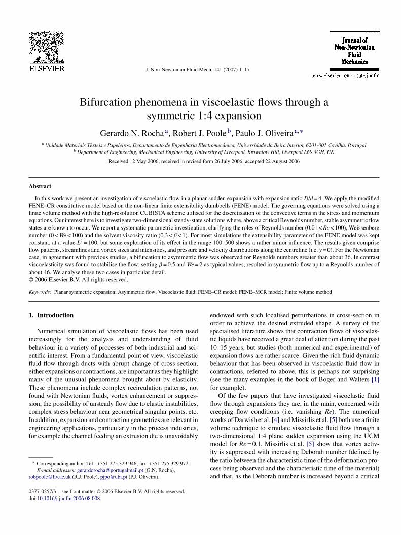
In the current study we present a systematic numerical inves-igation of the flow of a FENE–MCR liquid in a planar suddenxpansion of expansion ratio 4. The basic elements of laminarow, with moderate inertia, Re O(50) say, through a planar sud-en expansion are illustrated in Fig. 1. The flow progresses fromeing fully developed at a plane some distance L1 upstream fromhe expansion to being fully developed in the downstream chan-el at a distance L2 from the expansion plane. The exact shape ofhe recirculation regions may be concave or convex with respecto the expansion corner, depending if the flow is dominatedy viscous or inertial forces, respectively. The purpose of theresent work is to provide quantitative data of benchmark qual-ty for the flow through a 1:4 planar expansion of viscoelasticiquids obeying the constant viscosity FENE–MCR constitutive

odel.The main objectives of the present study are: (i) to exam-

ne the possible effects of each non-dimensional parameter (i.e.e, We and β) of the FENE–MCR model upon the flow andompare with the results of Oliveira [11] for a planar suddenxpansion of lower expansion ratio of 1:3; (ii) to investigate theritical Reynolds number of the symmetry-breaking bifurcationnd flow asymmetries occurring in plane sudden expansions forewtonian and viscoelastic fluids; (iii) to analyse the effect of

lasticity on the flow field; (iv) to show the variation of profilesf the velocity, stress and pressure along the centreline for theewtonian and viscoelastic cases.

. Conservation and constitutive equations

In the present work we consider the two-dimensional isother-al flow of an incompressible liquid flowing from a straight

hannel of height d to a larger channel of height D = 4d, cor-

esponding to an expansion ratio D/d = 4. In consequence, therocess generates a complex flow exhibiting regions of stronghearing near the walls and uniaxial planar extension alonghe centreline. The upstream channel where the cross-section

ic of expected flow patterns for moderate Re (O(50)).

onian

aslffl

a

∇

ρ

wcDttn

wt

τ

vc

epbcnv

τ

w

f

remE

∇τ

asiCsfFap

(TCtImRsHfidv

w

•

•

••

3

teitrtcu(lri

tssngfr

ioicvta

G.N. Rocha et al. / J. Non-Newt

verage velocity is U, has a length of L1 = 20d and the down-tream channel a length L2 = 50d, as show in Fig. 1. Theseengths are required for the establishment of a clear region ofully developed flow upstream of the expansion, and completeow redevelopment downstream of it.

This problem is governed by the usual equations of continuitynd motion, which can be written as [12]:

· u = 0 (1)

Du

Dt= −∇p+ ∇ · τtot (2)

here u is the local velocity vector, ρ the fluid density (assumedonstant), p the pressure, τtot the total extra stress tensor, and( )/Dt = ∂( )/∂t + u·�( ) is the substantial derivative, or deriva-

ive following the motion. For a homogeneous polymeric solu-ion the extra stress can be decomposed by the sum of a Newto-ian solvent and a polymeric solute contribution (τtot = τs + τ).

The Newtonian solvent component is expressed in Eq. (3),here the solvent viscosity ηs is constant, �uT the transpose of

he velocity gradient, and D is the rate-of-strain tensor.

s = ηs(∇u + ∇uT) ≡ 2ηsD (3)

When the fluid is viscoelastic (i.e. it presents simultaneouslyiscous and elastic properties), the problem is considerably moreomplicated compared to the Newtonian case.

In the current study we use a modified form of the finitextensibility non-linear dumbbells (FENE [13]) model, valid forolymeric materials, the so-called FENE–CR model, proposedy Chilcott and Rallison [14]. The FENE–CR model predictsonstant shear viscosity, η0 = ηp + ηs, shear-thinning of the firstormal-stress difference coefficient and bounded elongationaliscosity (proportional to L2) and is given by:

+ λ

f (τ)∇τ = 2ηpD (4)

ith the stretch function f(τ) expressed by:

(τ) = L2 + (λ/ηp)tr(τ)

L2 − 3(5)

In the previous equations, tr is the trace operator, λ a constantelaxation time, ηp the polymer viscosity (constant) and L2 is thextensibility parameter that measures the size of the polymerolecule in relation to its equilibrium size. The symbol ‘�’ inq. (4) is used to denote Oldroyd’s upper convected derivate:

= Dτ

Dt− τ · ∇u − ∇uT · τ (6)

nd the superscript ‘T’ in Eq. (6) denotes the transpose of a ten-or. In the current study an additional simplification is embodiedn Eq. (4), compared with the original FENE–CR equation ofhilcott and Rallison [14], in that the term D(1/f)/Dt is con-

idered to be negligible. This model is denoted FENE–MCR,

or modified Chilcott–Rallison model. The FENE–CR andENE–MCR models are identical in simple steady-state flowsnd the only difference between the two models occurs in com-lex transient flows, where the effect of the neglected term

cead

Fluid Mech. 141 (2007) 1–17 3

u·�(1/f)) can be important only in strong convective flows.he FENE–MCR model has been used in previous works byoates et al. [15] in a numerical study of axisymmetric contrac-

ion flow and more recently by the related study of Oliveira [11].n other works Oliveira has shown that results from those twoodels are virtually undistinguishable in complex flows at loweynolds numbers and since we wanted to compare the present

imulations with those of [11] we decided to use the MCR model.owever, some calculations were undertaken with the unmodi-ed CR model (Eq. (4), with the f(τ) function inside the Oldroyderivative) which lead essentially to the same results, with onlyery minor quantitative deviations with increasing Re.

The relevant non-dimensional parameters to be varied in thisork are:

L2, the extensibility parameter of the FENE–CR model (basevalue fixed at L2 = 100);β = ηs/η0, the solvent viscosity ratio, where the global shearviscosity is η0 = ηs + ηp (constant);Re = ρUd/η0, the Reynolds number;We = λU/d, the Weissenberg number.

. Numerical method

As mentioned previously, the numerical method applied inhis work is the finite volume method (FVM). The governingquations (Eqs. (1), (2), (4) and (5)) are discretised in space byntegration over the set of control volumes forming the computa-ional mesh, and in time over a small time step,�t. This processesults in systems of linearised algebraic equations for the equa-ions of mass and momentum conservation jointly with theonstitutive equation. In these equations all variables are eval-ated and stored in the central position of the control volumescells) and the computational mesh applied for the present simu-ations is orthogonal. As a consequence, special procedures areequired to ensure the pressure/velocity coupling and the veloc-ty/stress coupling (following the Oliveira et al. method [16]).

For the calculation of the convective terms in both the consti-utive Eq. (4) and the momentum Eq. (2) we use a high-resolutioncheme called CUBISTA [17], with third-order accuracy inpace for smooth flow, and having simultaneously both highumerical precision and good characteristics of iterative conver-ence. The CUBISTA scheme is implemented explicitly, exceptor the part corresponding to upwind fluxes which are incorpo-ated implicitly through the coefficients.

The constitutive and the momentum conservation equationsn discretised form are solved using a modified algorithm basedn the SIMPLE algorithm developed by Patankar and Spald-ng [18] that allows, through an iterative process of pressureorrection, to guarantee the coupling of velocity and pressure,erifying the continuity equation. The presence of the consti-utive equation for the viscoelastic fluid requires some minorlterations to the original SIMPLE method, which are mainly

oncerned with the calculation of pressure from the continuityquation. Two new steps are introduced in the initial part of thelgorithm to account for the stress equation; this procedure isocumented in detail elsewhere [16].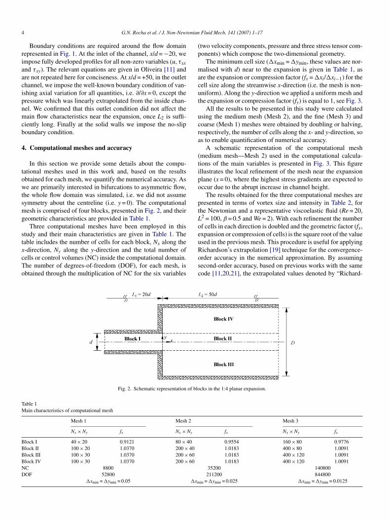

4 tonian

riaacipnmcb

4

towtsmg

stxcTo

(p

macut

ucra

(tipo

ptLoeu

TM

BBBBND

G.N. Rocha et al. / J. Non-New

Boundary conditions are required around the flow domainepresented in Fig. 1. At the inlet of the channel, x/d = −20, wempose fully developed profiles for all non-zero variables (u, τxx

nd τxy). The relevant equations are given in Oliveira [11] andre not repeated here for conciseness. At x/d = +50, in the outlethannel, we impose the well-known boundary condition of van-shing axial variation for all quantities, i.e. ∂/∂x = 0, except theressure which was linearly extrapolated from the inside chan-el. We confirmed that this outlet condition did not affect theain flow characteristics near the expansion, once L2 is suffi-

iently long. Finally at the solid walls we impose the no-slipoundary condition.

. Computational meshes and accuracy

In this section we provide some details about the compu-ational meshes used in this work and, based on the resultsbtained for each mesh, we quantify the numerical accuracy. Ase are primarily interested in bifurcations to asymmetric flow,

he whole flow domain was simulated, i.e. we did not assumeymmetry about the centreline (i.e. y = 0). The computationalesh is comprised of four blocks, presented in Fig. 2, and their

eometric characteristics are provided in Table 1.Three computational meshes have been employed in this

tudy and their main characteristics are given in Table 1. Theable includes the number of cells for each block, Nx along the

-direction, Ny along the y-direction and the total number ofells or control volumes (NC) inside the computational domain.he number of degrees-of-freedom (DOF), for each mesh, isbtained through the multiplication of NC for the six variables

Rosc

Fig. 2. Schematic representation of blo

able 1ain characteristics of computational mesh

Mesh 1 Mesh 2

Nx × Ny fx Nx × Ny

lock I 40 × 20 0.9121 80 × 40lock II 100 × 20 1.0370 200 × 40lock III 100 × 30 1.0370 200 × 60lock IV 100 × 30 1.0370 200 × 60C 8800OF 52800

�xmin =�ymin = 0.05 �xm

Fluid Mech. 141 (2007) 1–17

two velocity components, pressure and three stress tensor com-onents) which compose the two-dimensional geometry.

The minimum cell size (�xmin =�ymin, these values are nor-alised with d) near to the expansion is given in Table 1, as

re the expansion or compression factor (fx =�xi/�xi−1) for theell size along the streamwise x-direction (i.e. the mesh is non-niform). Along the y-direction we applied a uniform mesh andhe expansion or compression factor (fy) is equal to 1, see Fig. 3.

All the results to be presented in this study were calculatedsing the medium mesh (Mesh 2), and the fine (Mesh 3) andoarse (Mesh 1) meshes were obtained by doubling or halving,espectively, the number of cells along the x- and y-direction, sos to enable quantification of numerical accuracy.

A schematic representation of the computational meshmedium mesh—Mesh 2) used in the computational calcula-ions of the main variables is presented in Fig. 3. This figurellustrates the local refinement of the mesh near the expansionlane (x = 0), where the highest stress gradients are expected toccur due to the abrupt increase in channel height.

The results obtained for the three computational meshes areresented in terms of vortex size and intensity in Table 2, forhe Newtonian and a representative viscoelastic fluid (Re = 20,2 = 100, β = 0.5 and We = 2). With each refinement the numberf cells in each direction is doubled and the geometric factor (fx,xpansion or compression of cells) is the square root of the valuesed in the previous mesh. This procedure is useful for applying

ichardson’s extrapolation [19] technique for the convergence-rder accuracy in the numerical approximation. By assumingecond-order accuracy, based on previous works with the sameode [11,20,21], the extrapolated values denoted by “Richard-

cks in the 1:4 planar expansion.

Mesh 3

fx Nx × Ny fx

0.9554 160 × 80 0.97761.0183 400 × 80 1.00911.0183 400 × 120 1.00911.0183 400 × 120 1.0091

35200 140800211200 844800

in =�ymin = 0.025 �xmin =�ymin = 0.0125

G.N. Rocha et al. / J. Non-Newtonian Fluid Mech. 141 (2007) 1–17 5

he com

s(

rt0fltTefir

vawvchm

5

p

TE

(

(

W

eborotttaaoltctqtirwt

Fig. 3. Zoomed view of the medium mesh used in t

on’s extrapolation” are given in Table 2, for the vortices sizesXr) and intensities (ψr).

The discretisation errors on Mesh 2 (our base mesh for theemaining results) are also given in the previous table. It can seenhat the discretisation errors for the recirculation size are below.15% for the Newtonian fluid and 1.4% for the viscoelasticuid, while errors in recirculation intensity are below 0.7% for

he Newtonian fluid and 10.3% for the FENE–MCR simulations.he errors in ψr are much higher than errors in Xr because thevaluation of ψr requires integration of the resulting velocityelds and this integration tends to lower the accuracy of theesults (see Alves et al. [20]).

Thus, in general, the uncertainty in our directly calculatedalues is around 1–2% and the stress fields, in particular, whichre so important for the correct prediction of viscoelastic flows,ere observed to converge well with mesh refinement. For theiscoelastic case in Table 2 (i.e. part (b)) a detailed view ofontour plots of τxx predicted on the three meshes, not shownere for conciseness, confirms that the results of the two finereshes are almost coincident.

. Results and discussion

In this section we present and discuss our results and, from theoint of view of their practical utility, they may be classified as

able 2ffect of mesh refinement for Re = 20

Xr ψr (×10−2)

a) Newtonian caseMesh 1 3.6281 6.5039Mesh 2 3.6307 6.5487Mesh 3 3.6349 6.5827Richardson’s extrapolation 3.6363 6.5940Discretisation error (%) 0.15 0.69

b) Viscoelastic caseMesh 1 2.0684 2.2307Mesh 2 2.1562 2.6163Mesh 3 2.1787 2.8421Richardson’s extrapolation 2.1862 2.9174Discretisation error (%) 1.37 10.32

e = 2, β = 0.5 and L2 = 100.

a1so

5

niDrnrbwaiai

putational calculation (−2 ≤ x ≤ 10; −2 ≤ y ≤ 2).

ither qualitative or quantitative results. The qualitative results toe given essentially comprise streamline plots, an effective wayf illustrating the effect of inertia, elasticity and solvent viscosityatio on the degree of recirculation and observing the existence,r not, of asymmetric flow. In addition the main contribution ofhe work is however the quantitative analysis, which comprisesables and figures for the size and intensity of the corner vor-ex, stress distributions, velocity profiles and the pressure droplong the centreline. Our numerical values for the Newtoniannd viscoelastic fluid flows are also compared with the resultsbtained by Oliveira [11] for a planar sudden expansion with aower expansion ratio of 3. Firstly we document our results forhe Newtonian case with the main purpose of validating the cal-ulations. An equivalent validation could not be undertaken forhe viscoelastic simulations because we could not find an ade-uate data set in the literature for comparison. Next we considerhe viscoelastic case, for which we study the effects of elastic-ty, polymer concentration and inertia. In the current work L2

emains constant, at value of L2 = 100, in accordance with theork of Remmelgas et al. [22]. Section 5.2.3 discusses briefly

he influence of extensibility, in the range L2 = 100–500.All calculations presented in this work were conducted using

Pentium® IV personal computer with 3.0 GHz clock speed and024 MB random access memory. The computational time waseen to increase almost linearly with the mesh density (numberf cells).

.1. Results for the Newtonian case (validation)

In Fig. 4 we compare our predicted bifurcation results with theumerical values obtained in the work of Drikakis [2]. Follow-ng Drikakis we find it useful to define the parameter DX, whereX = (Xr1 − Xr2), to quantify the existence, or not, of asymmet-

ic flow. The parameter DX is zero for a symmetric flow andon-zero, with opposite signs, for the two possible asymmet-ic flow states after the critical Reynolds number. The upperranch in Fig. 4 corresponds to flow attaching first to the upperall and, conversely, the lower branch corresponds to the flow

ttaching to the lower wall. Drikakis analysed Newtonian flown several expansion ratios, imposing fully-developed conditionst inlet and defining the Reynolds number using the maximumnlet velocity (U0 = 1.5U) and height of the inlet channel (d).

6 G.N. Rocha et al. / J. Non-Newtonian

Fa

Waas

snb

TP

R

1

rt

w[laRtPTccfltNetv

aN1awest

ig. 4. Comparison of the bifurcation parameter DX between our simulationsnd the results of Drikakis [2] results for the Newtonian fluid.

e have reprocessed his results so the definitions used in Fig. 4re consistent with ours. Our results are, in the main, in goodgreement with the results of Drikakis except for a discernableystematic difference for Re > 45.

Our predicted results for a Newtonian fluid are also pre-

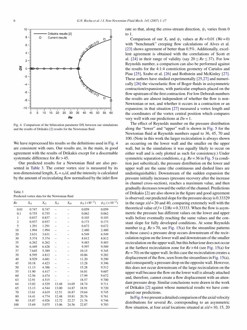
ented in Table 3. The corner vortex size is measured by itson-dimensional length, Xr = xr/d, and the intensity is calculatedy the amount of recirculating flow normalised by the inlet flow

able 3redicted vortex data for the Newtonian fluid

e Xr1 Xr2 Xr3 Xr4 ψrl (×l0−2) ψr2 (×10−2)

0.01 0.747 0.747 – – 0.059 0.0590.1 0.755 0.755 – – 0.062 0.0621 0.837 0.837 – – 0.103 0.1032 0.937 0.937 – – 0.173 0.1735 1.291 1.291 – – 0.672 0.672

10 1.994 1.994 – – 2.480 2.48020 3.631 3.631 – – 6.549 6.54930 5.374 5.374 – – 8.812 8.81235 6.262 6.262 – – 9.483 9.48336 6.449 6.428 – – 9.597 9.58937 7.645 5.389 – – 10.15 9.34539 8.595 4.812 – – 10.86 9.28240 8.929 4.681 – – 11.20 9.29045 10.18 4.423 – – 13.28 9.39650 11.13 4.386 – – 15.28 9.51255 11.90 4.417 – – 16.81 9.60760 12.56 4.474 – – 17.99 9.67263 12.91 4.515 – – 18.57 9.70064 13.02 4.529 13.48 14.05 18.74 9.71165 13.13 4.544 13.00 14.87 18.91 9.72070 13.61 4.619 12.51 16.87 19.64 9.74580 14.41 4.774 12.48 19.81 20.76 9.76190 15.07 4.926 12.72 22.27 21.76 9.74600 15.69 5.075 13.06 24.56 22.87 9.703

uupigoiitmwsnicraRdatuadop

dfl

Fluid Mech. 141 (2007) 1–17

ate so that, along the cross-stream direction, ψr varies from 0o 1.

Comparison of our Xr and ψr values at Re = 0.01 (We = 0)ith “benchmark” creeping flow calculations of Alves et al.

23] shows agreement of better than 0.5%. Additionally, excel-ent agreement is obtained with the correlations of Scott etl. [24] in their range of validity (say 20 ≤ Re ≤ 37). For loweynolds number, a comparison can also be performed against

he results for the 4:1:4 constriction geometry of Cartalos andiau [25], Szabo et al. [26] and Rothstein and McKinley [27].hese authors have studied experimentally [25,27] and numeri-ally [26] the viscoelastic flow of Boger fluids in axisymmetricontraction/expansions, with particular emphasis placed on theow upstream of the first contraction. For low Deborah numbers

he results are almost independent of whether the flow is non-ewtonian or not, and whether it occurs in a contraction or an

xpansion; in that situation [27] measured a vortex length andhe coordinates of the vortex central position which comparesery well with our predictions at De = 1.

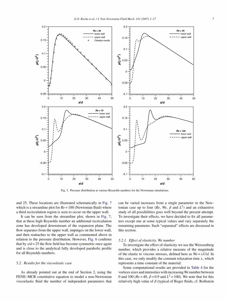
The effect of Reynolds number on the pressure distributionlong the “lower” and “upper” wall is shown in Fig. 5 for theewtonian fluid at Reynolds numbers equal to 36, 45, 70 and00. (Note in this work the larger recirculation is always showns occurring on the lower wall and the smaller on the upperall, but in the simulations it was equally likely to occur on

ither wall and is only plotted as such for consistency.) Underymmetric separation conditions, e.g. Re = 36 in Fig. 5 (a condi-ion just subcritical), the pressure distribution on the lower andpper wall are the same (the continuous and dashed lines arendistinguishable). Downstream of the sudden expansion theressure initially increases (pressure recovery after the increasen channel cross-section), reaches a maximum value, and thenradually decreases toward the outlet of the channel. Predictionsf Drikakis [2] are also shown in the figure and good agreements observed; our predicted slope for the pressure decay is 0.33329n the range x/d = 20 and 40, comparing extremely well with theheoretical value of f = 12/Re = 0.33333. When the flow is asym-

etric the pressure has different values on the lower and upperalls before eventually reaching the same values and the con-

tant slope for fully developed conditions. At some Reynoldsumber (e.g. Re > 70, see Fig. 15(a) for the streamline patternsn these cases) a pressure drop occurs downstream of the recir-ulation region on the lower wall and downstream of the smallerecirculation on the upper wall, but this behaviour does not occurt the farthest recirculation zone for Re > 64 (see Fig. 15(a) fore = 70) on the upper wall. In this case the recirculation creates aisplacement of the flow, seen from the streamlines in Fig. 15(a),nd consequently a pressure drop on the opposite wall. However,his does not occur downstream of the large recirculation on thepper wall because the flow on the lower wall is already attachednd, therefore, cannot create a flow displacement with an atten-ant pressure drop. Similar conclusions were drawn in the workf Drikakis [2] against whose numerical results we have com-

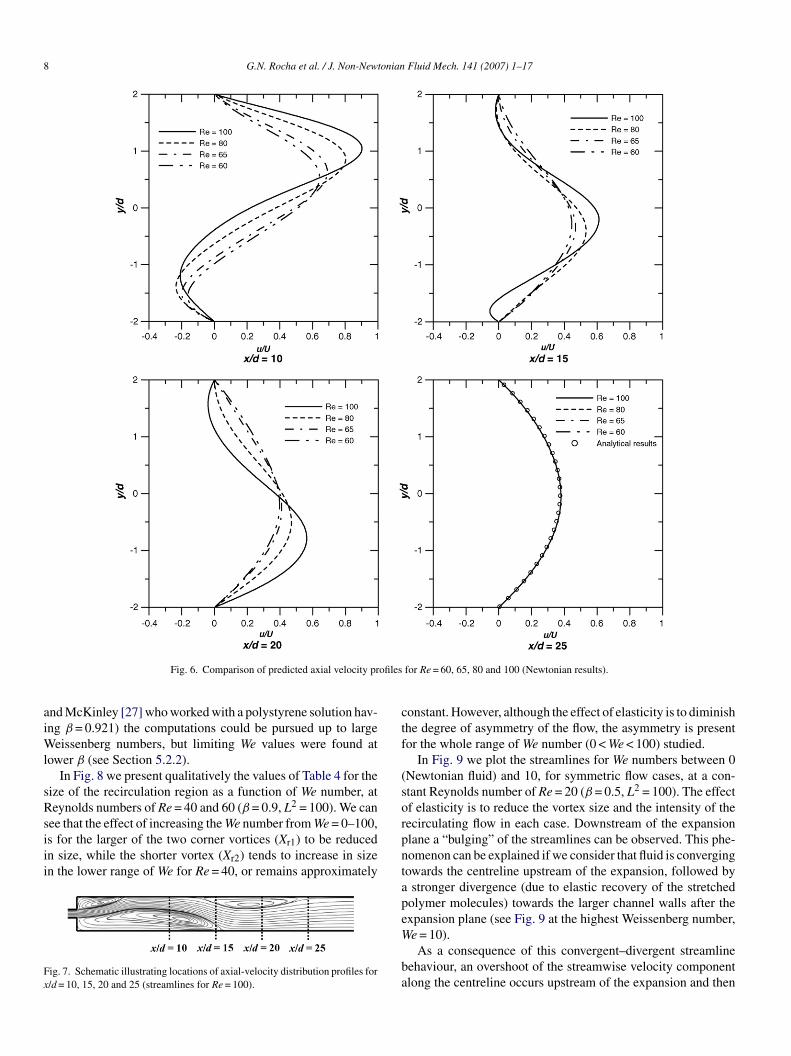
ared our predictions.

In Fig. 6 we present a detailed comparison of the axial velocityistributions for several Re, corresponding to an asymmetricow situation, at four axial locations situated at x/d = 10, 15, 20

G.N. Rocha et al. / J. Non-Newtonian Fluid Mech. 141 (2007) 1–17 7

nolds

awa

tzflartaf

5

Fv

ctsTtrt

5

notr

Fig. 5. Pressure distribution at various Rey

nd 25. These locations are illustrated schematically in Fig. 7hich is a streamline plot for Re = 100 (Newtonian fluid) wherethird recirculation region is seen to occur on the upper wall.

It can be seen from the streamline plot, shown in Fig. 7,hat at these high Reynolds number an additional recirculationone has developed downstream of the expansion plane. Theow separates from the upper wall, impinges on the lower wall,nd then reattaches to the upper wall as commented above inelation to the pressure distribution. However, Fig. 6 confirmshat by x/d = 25 the flow field has become symmetric once againnd is close to the analytical fully developed parabolic profileor all Reynolds numbers.

.2. Results for the viscoelastic case

As already pointed out at the end of Section 2, using theENE–MCR constitutive equation to model a non-Newtonianiscoelastic fluid the number of independent parameters that

v0r

numbers for the Newtonian simulations.

an be varied increases from a single parameter in the New-onian case up to four (Re, We, β and L2) and an exhaustivetudy of all possibilities goes well beyond the present attempt.o investigate their effects, we have decided to fix all parame-

ers except one at some typical values and vary separately theemaining parameter. Such “separated” effects are discussed inhis section.

.2.1. Effect of elasticity, We numberTo investigate the effect of elasticity we use the Weissenberg

umber, which provides a relative measure of the magnitudef the elastic to viscous stresses, defined here as We = λU/d. Inhis case, we only modify the constant relaxation time λ, whichepresents a time constant of the material.

Some computational results are provided in Table 4 for theortices sizes and intensities with increasing We number betweenand 100 (Re = 40, β = 0.9 and L2 = 100). We note that for this

elatively high value of β (typical of Boger fluids, cf. Rothstein

8 G.N. Rocha et al. / J. Non-Newtonian Fluid Mech. 141 (2007) 1–17

ofiles

aiWl

sRsiii

Fx

ctf

(so

Fig. 6. Comparison of predicted axial velocity pr

nd McKinley [27] who worked with a polystyrene solution hav-ng β = 0.921) the computations could be pursued up to large

eissenberg numbers, but limiting We values were found atower β (see Section 5.2.2).

In Fig. 8 we present qualitatively the values of Table 4 for theize of the recirculation region as a function of We number, ateynolds numbers of Re = 40 and 60 (β = 0.9, L2 = 100). We can

ee that the effect of increasing the We number from We = 0–100,s for the larger of the two corner vortices (Xr1) to be reducedn size, while the shorter vortex (Xr2) tends to increase in sizen the lower range of We for Re = 40, or remains approximately

ig. 7. Schematic illustrating locations of axial-velocity distribution profiles for/d = 10, 15, 20 and 25 (streamlines for Re = 100).

rpntapeW

ba

for Re = 60, 65, 80 and 100 (Newtonian results).

onstant. However, although the effect of elasticity is to diminishhe degree of asymmetry of the flow, the asymmetry is presentor the whole range of We number (0 < We < 100) studied.

In Fig. 9 we plot the streamlines for We numbers between 0Newtonian fluid) and 10, for symmetric flow cases, at a con-tant Reynolds number of Re = 20 (β = 0.5, L2 = 100). The effectf elasticity is to reduce the vortex size and the intensity of theecirculating flow in each case. Downstream of the expansionlane a “bulging” of the streamlines can be observed. This phe-omenon can be explained if we consider that fluid is convergingowards the centreline upstream of the expansion, followed bystronger divergence (due to elastic recovery of the stretched

olymer molecules) towards the larger channel walls after thexpansion plane (see Fig. 9 at the highest Weissenberg number,

e = 10).As a consequence of this convergent–divergent streamline

ehaviour, an overshoot of the streamwise velocity componentlong the centreline occurs upstream of the expansion and then

G.N. Rocha et al. / J. Non-Newtonian Fluid Mech. 141 (2007) 1–17 9

symm

afLaestisstint(

flfaTntt

Fbi

Fig. 8. Effect of Weissenberg number on the size of the two a

n undershoot occurs downstream. This behaviour is shown,or the particular case of Re = 20 and We = 0 and 10 (β = 0.5,2 = 100), in Fig. 10 where it is clear that the fluid accelerationlong the centreline is concentrated in a small region just at thentrance to the expansion (x ≈ 0), while the region of divergingtreamlines is distributed over a longer distance downstream ofhe expansion plane. The effect becomes more pronounced withncreasing We, but is also dependent on the Reynolds number, ashown in Fig. 11 for We = 2 and We = 4. From this figure, whichhows the variation of these velocity over and undershoots alonghe centreline with Re, it is clear that the overshoot of veloc-

ty near the expansion plane increases with increasing elasticityumber (E = λη0/ρd2 = (1 −β)We/Re) and that the undershoot inhe diverging streamlines zone reaches a maximum at a given E≈0.08–0.10). A nice and definite explanation for this “diverging

Ttid

Fig. 9. Streamlines at various We numbe

etric vortices (L2 = 100, β = 0.9): (a) Re = 40 and (b) Re = 60.

ow behaviour” was recently put forth by Alves and Poole [28]or the contraction flow case, but the same mechanism should bet work for the sudden expansion case under consideration here.heir analysis demonstrated that inertia (through the Reynoldsumbers) is not necessary for diverging flow to be observed:herefore the phenomenon should not be directly controlled byhe elasticity number.

A peculiar feature in the vortex size variation with We seen inig. 8 for the lower Re value (Re = 40) is worth discussing hereecause it is an elastic effect that was, in fact, already presentn the work of Oliveira [11] (see his Fig. 8) but went unnoticed.

here is a slight, but distinct, dip in the size of the smallest vor-

ex (Xr2) at We = 45 (Re = 40 ⇒ E ≈ 0.1), with an ensuing slightncrease of Xr1. In order to clarify the origin of such a small, butiscernable ‘kink’ in the variation of Xr, we plot the streamlines

rs (Re = 20, L2 = 100, and β = 0.5).

10 G.N. Rocha et al. / J. Non-Newtonian Fluid Mech. 141 (2007) 1–17

Table 4Predicted vortex data for the viscoelastic fluid/Effect of elasticity through We,for Re = 40, β = 0.9 and L2 = 100

We Xr1 Xr2 ψr1 (×10−2) ψr2 (×10−2)

0 8.93 4.68 11.20 9.291 8.44 4.96 10.50 9.052 8.10 5.09 10.28 8.983 7.99 5.02 10.30 8.924 7.96 4.92 10.38 8.855 7.95 4.84 10.45 8.78

10 7.90 4.62 10.60 8.5215 7.85 4.54 10.59 8.4020 7.83 4.49 10.55 8.3630 7.82 4.43 10.49 8.5040 7.83 4.36 10.44 8.7850 7.91 4.20 10.16 9.6660 7.92 4.27 10.11 9.8070 7.92 4.28 10.10 9.9180 7.93 4.28 10.10 9.92

1

f(avsWias

5

tt

FRL

90 7.93 4.28 10.10 9.9200 7.93 4.28 10.10 9.92

or the Re of interest in Fig. 12. It appears that for We ≥ 45E ≥ 0.11) the shape of the smaller vortex near the wall changesbruptly from an elongated shape, typical of the Newtonianortex (cf. We = 0), to a more strongly convex shape, with theeparation streamline now intersecting the wall at a right angle.e hypothesise that this elastic retraction of the smaller vortex

s related to the “diverging streamlines” phenomenon discussedbove. For Re = 60 (We = 2, β = 0.9, E = (1 – 0.9) × 2/60 = 0.003)uch a perturbation in vortex size is absent, as seen in Fig. 8(b).

.2.2. Effect of concentration, βThe β parameter measures the ratio of solvent viscosity to

otal shear viscosity. For the present study we varied β from 1.0o 0.3, at fixed Re = 40, We = 2 and L2 = 100.

ig. 10. Variation of streamwise velocity component along the centerline fore = 20 at We = 0 (Newtonian fluid) and We = 10 (viscoelastic fluid, β = 0.5 and2 = 100).

Fb(

oi

t

TPβ

β

10000000

ig. 11. Variation of the velocity overshoot and undershoot with Reynolds num-er for two Weissenberg numbers (L2 = 100): (a) We = 2 (β = 0.5 and 0.8) andb) We = 4 (β = 0.5).

The numerical results of the present parametric study, in terms

f vortex size and intensity, are given in Table 5 and qualitativelyllustrated in Fig. 13.

Analysing Fig. 13 we can see that for a decreasing β ratiohe flow is stabilized until a stable symmetrical state exists

able 5redicted vortex data for the viscoelastic fluid/Effect of concentration parameter, for We = 2, Re = 40 and L2 = 100

Xr1 Xr2 ψr1 (×10−2) ψr2 (×10−2)

.0 8.929 4.681 11.20 9.290

.9 8.101 5.086 10.28 8.983

.8 6.644 6.129 9.189 8.967

.7 5.993 6.059 8.601 8.639

.6 5.659 5.693 8.158 8.178

.5 5.319 5.336 7.662 7.671

.4 4.979 4.989 7.035 7.041

.3 4.651 4.659 6.321 6.325

G.N. Rocha et al. / J. Non-Newtonian Fluid Mech. 141 (2007) 1–17 11

L2 = 1

frhrttd

rna

Fig. 12. Vortex shapes at increasing Weissenberg number (β = 0.9 and

or values of β≤ 0.8, at Re = 40, while the flow is asymmet-ic for β > 0.8. It is clear that the Newtonian flow (β = 1.0)as the largest asymmetry and this asymmetry is somewhat

educed with a small introduction of elasticity in the fluid,hrough the β parameter, and it is completely attenuated whenhe concentration is further increased. Following the practice ofefining the Weissenberg number based on a Maxwell model

tise

00) and constant Reynolds number (Re = 40). Note change at We = 45.

elaxation time (that is, λ0 =ψ1/2η0, where ψ1 is the firstormal-stress coefficient), the influence of β can be seen asn elastic effect provided we use We′ = We(1 −β) to define

he Weissenberg number. For β = 1 we have We′ = 0 and nonfluence of viscoelasticity is expected; for β < 1, with progres-ively lower values, We′ increases implying higher levels oflasticity.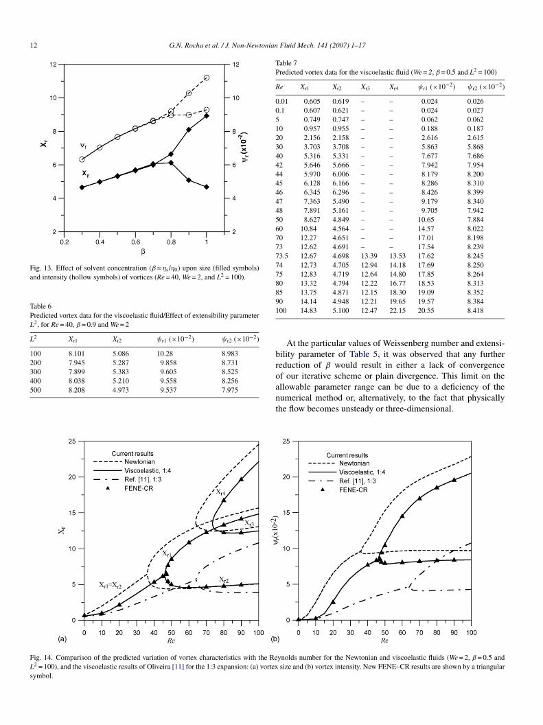

12 G.N. Rocha et al. / J. Non-Newtonian Fluid Mech. 141 (2007) 1–17

Fig. 13. Effect of solvent concentration (β = ηs/η0) upon size (filled symbols)and intensity (hollow symbols) of vortices (Re = 40, We = 2, and L2 = 100).

Table 6Predicted vortex data for the viscoelastic fluid/Effect of extensibility parameterL2, for Re = 40, β = 0.9 and We = 2

L2 Xr1 Xr2 ψr1 (×10−2) ψr2 (×10−2)

100 8.101 5.086 10.28 8.983200 7.945 5.287 9.858 8.731345

Table 7Predicted vortex data for the viscoelastic fluid (We = 2, β = 0.5 and L2 = 100)

Re Xr1 Xr2 Xr3 Xr4 ψr1 (×10−2) ψr2 (×10−2)

0.01 0.605 0.619 – – 0.024 0.0260.1 0.607 0.621 – – 0.024 0.0275 0.749 0.747 – – 0.062 0.06210 0.957 0.955 – – 0.188 0.18720 2.156 2.158 – – 2.616 2.61530 3.703 3.708 – – 5.863 5.86840 5.316 5.331 – – 7.677 7.68642 5.646 5.666 – – 7.942 7.95444 5.970 6.006 – – 8.179 8.20045 6.128 6.166 – – 8.286 8.31046 6.345 6.296 – – 8.426 8.39947 7.363 5.490 – – 9.179 8.34048 7.891 5.161 – – 9.705 7.94250 8.627 4.849 – – 10.65 7.88460 10.84 4.564 – – 14.57 8.02270 12.27 4.651 – – 17.01 8.19873 12.62 4.691 – – 17.54 8.23973.5 12.67 4.698 13.39 13.53 17.62 8.24574 12.73 4.705 12.94 14.18 17.69 8.25075 12.83 4.719 12.64 14.80 17.85 8.26480 13.32 4.794 12.22 16.77 18.53 8.31385 13.75 4.871 12.15 18.30 19.09 8.35291

br

FLs

00 7.899 5.383 9.605 8.52500 8.038 5.210 9.558 8.25600 8.208 4.973 9.537 7.975

oant

ig. 14. Comparison of the predicted variation of vortex characteristics with the Re2 = 100), and the viscoelastic results of Oliveira [11] for the 1:3 expansion: (a) vortexymbol.

0 14.14 4.948 12.21 19.65 19.57 8.38400 14.83 5.100 12.47 22.15 20.55 8.418

At the particular values of Weissenberg number and extensi-ility parameter of Table 5, it was observed that any furthereduction of β would result in either a lack of convergence

f our iterative scheme or plain divergence. This limit on thellowable parameter range can be due to a deficiency of theumerical method or, alternatively, to the fact that physicallyhe flow becomes unsteady or three-dimensional.

ynolds number for the Newtonian and viscoelastic fluids (We = 2, β = 0.5 andsize and (b) vortex intensity. New FENE–CR results are shown by a triangular

onian

5

dmI

c

G.N. Rocha et al. / J. Non-Newt

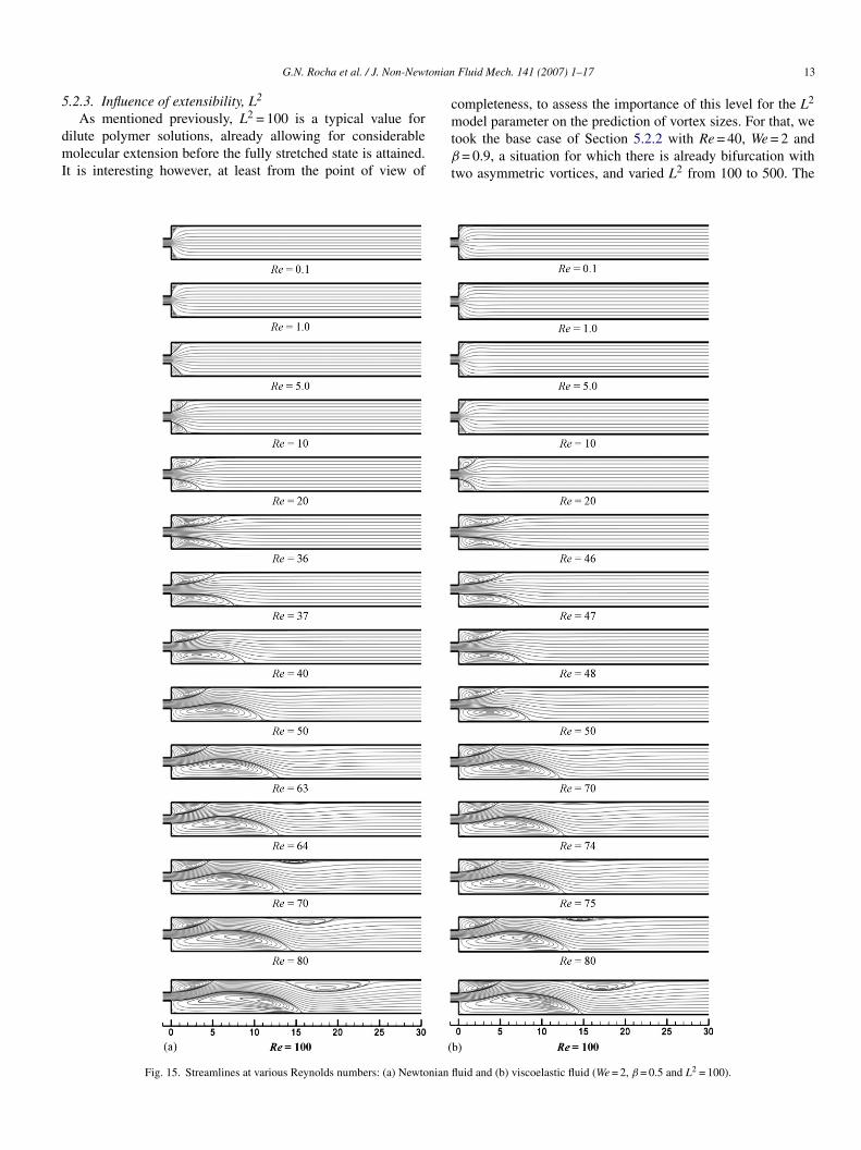
.2.3. Influence of extensibility, L2

As mentioned previously, L2 = 100 is a typical value forilute polymer solutions, already allowing for considerableolecular extension before the fully stretched state is attained.

t is interesting however, at least from the point of view of

mtβ

t

Fig. 15. Streamlines at various Reynolds numbers: (a) Newtonian fl

Fluid Mech. 141 (2007) 1–17 13

ompleteness, to assess the importance of this level for the L2

odel parameter on the prediction of vortex sizes. For that, weook the base case of Section 5.2.2 with Re = 40, We = 2 and= 0.9, a situation for which there is already bifurcation with

wo asymmetric vortices, and varied L2 from 100 to 500. The

uid and (b) viscoelastic fluid (We = 2, β = 0.5 and L2 = 100).

14 G.N. Rocha et al. / J. Non-Newtonian

Fa

cfoeL

5

aasR

vf

popcruwFrflraiiflac

Fssalaue

ig. 16. Bifurcation diagrams for Newtonian and viscoelastic (We = 2, β = 0.5nd L2 = 100) flows in a 1:4 planar expansion.

orresponding vortex size and intensity barely varied as seenrom Table 6, with a systematic small decrease of the intensityf both vortices, as expected from an increase in extensionallasticity. In conclusion, the influence of L2 on the flow, when2 is larger than 100, appears to be minimal.

.2.4. Effect of inertia, Re numberIn this section we present the results concerned with the vari-

tion of Reynolds number, for typical values L2 = 100, We = 2nd a moderate concentration β = 0.5. A Reynolds number mea-ures the ratio between the viscous and inertial forces. At highe values the flow is dominated by inertial forces and for low Re

fa

a

Fig. 17. Non-dimensional contour lines for the first normal-stress differenc

Fluid Mech. 141 (2007) 1–17

alues the flow is dominated by viscous forces and the inertialorces are less significant.

Our numerical data are provided in Table 7 and the values arelotted in Fig. 14(a), which shows the variation of the lengthsf the upper and lower vortices downstream of the expansionlane with Reynolds number and in Fig. 14(b), which shows theorresponding recirculation intensities. At very low Re, someather small differences are seen in Table 7 between the val-es of the two, nominally identical, vortex sizes but they areithin the numerical uncertainty (≈0.2–2.0%) of our results.or a Reynolds number up to a critical value (Recr = 46) the flowemains steady and symmetric, while for higher Re number theow is still steady but asymmetric with a larger and a smallerecirculation. For Re above 73.5 a further recirculation regionppears on either wall. In Fig. 15 we plot the streamlines for var-ous Reynolds numbers to highlight these effects. Additionally,n Fig. 14 we include the results of [11] for a similar viscoelasticuid model in a 1:3 expansion to illustrate the effects broughtbout by a reduction in expansion ratio: essentially a delayedritical bifurcation point and smaller and less intense vortices.

Another issue is whether the modification introduced in theENE–CR model (MCR against CR, cf. Section 2) producesignificant differences. The triangular symbols in Fig. 14 corre-pond to test calculations performed with the actual CR modelnd it may be concluded that minimal differences are seen forow to moderate Re, up to and around the bifurcation point,nd the discrepancies remain small at higher Re. Previous sim-lations with inertialess flows showed the two models to yieldssentially the same results. Thus, the conclusions drawn here

or the FENE–MCR model can, in general, be extended to thectual CR version of the FENE model.

In Fig. 16 we show the “bifurcation” plot (i.e. the vari-tion of the DX parameter with Re) for the viscoelastic

es (N1) with increasing We numbers (Re = 20, β = 0.5 and L2 = 100).

G.N. Rocha et al. / J. Non-Newtonian Fluid Mech. 141 (2007) 1–17 15

τxy) w

lfl

suRTovuo

stifl

ls

Fig. 18. Non-dimensional contour lines for the shear stress (

iquid, and compare to the equivalent data for the Newtonianuid.

From our results we can conclude that the transition from aymmetric to an asymmetric state is delayed to higher Re val-es by elasticity, specifically from Recr = 36 (Newtonian case) toecr = 46 (viscoelastic case) for this parameter set (see Fig. 14).he effect of elasticity is therefore a stabilizing factor for the

ccurrence of bifurcation, under steady flow conditions. Theortex sizes and intensities are smaller for the viscoelastic liq-id when compared with the Newtonian fluid. This effect isbserved for the whole range of Re, from 0 to 100, and can be

2

ca

Fig. 19. (a and b) Normal-stress profile τxx and τyy, along the centreline

ith increasing We numbers (Re = 20, β = 0.5 and L2 = 100).

een in Fig. 15(a and b) which shows the streamline plots forhe Newtonian and viscoelastic fluid, respectively. In this figuret is also possible to appreciate the phenomenon of ‘diverging’ow commented upon above.

In Figs. 17 and 18 we present the non-dimensional contourines for the first normal-stress differences (N1 = τxx − τyy) andhear stress (τxy), with increasing Weissenberg number (We = 0,

, 5 and 10) for Re = 20 (β = 0.5 and L2 = 100).

Globally these figures illustrate the higher level of stress con-entration for the viscoelastic fluid, both in respect of the normalnd shear components. The stress profiles are still symmetric,

(y = 0), for the viscoelastic fluid (Re = 20, β = 0.5 and L2 = 100).

16 G.N. Rocha et al. / J. Non-Newtonian Fluid Mech. 141 (2007) 1–17

iscoel

dcdoptagd

τ

bacss(tatnutdto

icoetlopA

isccsd

6

dsacmw(cre7srflt(oln

ii

Fig. 20. Pressure distribution along the centreline for the Newtonian and v

emonstrating that for the low Re numbers cases shown the bifur-ation phenomenon is not sensed by the stress field. Anotheretail is the displacement of the maximum stress downstreamf the expansion (see Fig. 17 for We = 2). The convective termsresent in the stress equations tend to sweep the stresses alonghe flow direction even if the Reynolds number is kept constants is the situation for the cases shown. Lastly, we can see theradual stress concentration near to the expansion corner as theegree of elasticity increases.

In Fig. 19 we plot the variation of the normal stresses τxx andyy along the centreline (i.e. y = 0), at several Weissenberg num-ers (We = 0, 1, 2 and 5) for the viscoelastic fluid (Re = 20,β = 0.5nd L2 = 100). The normal stresses are non-dimensionalised by aonvective scale,ρ * U2 and for the viscoelastic cases the stresseshown correspond to the polymeric contribution only. We canee a gradual increase of the maximum transverse normal-stressτyy > 0), and the location of this maximum value moves fur-her downstream with increasing elasticity. This behaviour is

consequence of a history (or memory) effect in the consti-utive equation. The τyy contribution is dominant in the firstormal-stress term (i.e. N1 = τxx − τyy) calculation and the val-es obtained from the stress components in Fig. 19 correspondo the elliptic region of maximum negative first normal-stressifferences seen in the contours of Fig. 17, thus explaining theendency for the lateral bulging of a fluid element seen previ-usly (Figs. 9 and 15).

In Fig. 20 we investigate the influence of viscoelasticity andnertia on the pressure distribution along the centreline of thehannel (y = 0) for the Newtonian and viscoelastic cases. A mem-ry effect in the fluid can again be observed downstream of thexpansion plane as a continuation of the pressure decrease forhe viscoelastic liquid. Indeed, for this type of fluid we can see a

ower minimum pressure, occurring slightly further downstreamf the expansion compared with the Newtonian fluid, for whichressure recovery starts immediately at the expansion plane.dditionally the pressure recovery, after the expansion zone,

fewn

astic fluids (We = 20, β = 0.5 and L2 = 100), at: (a) Re = 20 and (b) Re = 50.

s lower for the viscoelastic fluid, i.e. there is an enhanced pres-ure drop for the viscoelastic cases compared to the Newtonianase. This is an interesting result because for the correspondingontraction flow geometry, the predictions of several similar con-titutive models have consistently exhibited a reduced pressurerop for viscoelastic fluids (see Alves et al. [23] for example).

. Conclusions

Numerical simulations were conducted for flow in a two-imensional channel with a 1:4 sudden symmetric expansion. Aymmetry-breaking bifurcation was found for both Newtoniannd viscoelastic fluids, at different Reynolds numbers in eachase, and represents the transition from a symmetric to an asym-etric flow. The critical Reynolds numbers at the bifurcationere Recr = 36 and 46 for the Newtonian and viscoelastic fluids

L2 = 100, We = 2 andβ = 0.5), respectively. It was shown that theritical Reynolds number decreased with increasing expansionatio, compared with the work of Oliveira [11] for a 1:3 suddenxpansion. At higher Reynolds numbers, Re higher than 64 or3.5 for the Newtonian and viscoelastic liquid, respectively, aecond bifurcation point is observed and a further recirculationegions on the “upper” wall. This effect was not observed forows in the 1:3 expansion for Re < 100. Comparing the New-

onian and viscoelastic fluid simulations the effect of elasticitymeasured by the Weissenberg number) tends to delay the onsetf the bifurcation, and the vortex length and intensity are alwaysower for the viscoelastic fluid when compared with the Newto-ian case.

Similar conclusions can be drawn when the actual CR models used instead of its modified version, which is mostly employedn this investigation. A comparison between these two versions

or the constant viscosity FENE fluid shows almost no differ-nces at low Re, up to and above the critical bifurcation point,ith no systematic deviation for the CR at higher Reynoldsumbers.

onian

iaewlfsea

A

Ft

R

[

[

[

[

[

[

[

[

[

[

[

[

[

[

[

[

[

G.N. Rocha et al. / J. Non-Newt

It was seen that the inertial forces, through the Re number,ncrease the length and intensity of the vortex for both Newtoniannd viscoelastic fluids. In particular for the viscoelastic fluids theffect of Re was inhibited in a lower range (say Re = 0 − 10), inhich the vortex size and intensity are unaffected by inertia, fol-

owed by the inertial range that parallels the Newtonian tendencyor vortex enhancement. Finally, the polymer concentration waseen to have a very strong effect and for β > 0.8, at Re = 40 forxample, the flow was asymmetric but for lower values of β thesymmetry was completely removed.

cknowledgement

The authors would like to thank the financial support byundacao para a Ciencia e a Tecnologia (FCT), Portugal, through

he projects POCTI/EQU/37699/2001 and BD/22644/2005.

eferences

[1] D.V. Boger, K. Walters, Rheological Phenomena in Focus, Rheology Series,vol. 4, Elsevier, 1993.

[2] D. Drikakis, Bifurcation phenomena in incompressible sudden expansionflows, Phys. Fluids 9 (1997) 76–86.

[3] F. Battaglia, S.J. Tavener, A.K. Kulkarni, C.L. Merkle, Bifurcation of lowReynolds number flows in symmetric channels, AIAA J. 35 (1997) 99–105.

[4] M.S. Darwish, J.R. Whiteman, M.J. Bevis, Numerical modelling of vis-coelastic liquids using a finite-volume method, J. Non-Newtonian FluidMech. 45 (1992) 311–337.

[5] K.A. Missirlis, D. Assimacopoulos, E. Mitsoulis, A finite volume approachin the simulation of viscoelastic expansion flows, J. Non-Newtonian FluidMech. 78 (1998) 91–118.

[6] P. Townsend, K. Walters, Expansion flows of non-Newtonian liquids,Chem. Eng. Sci. 49 (1994) 749–763.

[7] A. Baloch, P. Townsend, M.F. Webster, On vortex development in vis-coelastic expansion and contraction flows, J. Non-Newtonian Fluid Mech.65 (1996) 133–149.

[8] D.E. Abbott, S.J. Kline, Experimental investigation of subsonic turbulentflow over single and double backward facing steps, J. Basic Eng. 84 (1962)317–325.

[9] W. Cherdron, F. Durst, J.H. Whitelaw, Asymmetric flows and instabilities in

symmetric ducts with sudden expansions, J. Fluid Mech. 84 (1978) 13–31.

10] F. Durst, J.C.F. Pereira, C. Tropea, The plane symmetric sudden-expansionflow at low Reynolds numbers, J. Fluid Mech. 248 (1993) 567–581.

11] P.J. Oliveira, Asymmetric flows of viscoelastic fluids in symmetric planarexpansion geometries, J. Non-Newtonian Fluid Mech. 114 (2003) 33–63.

[

[

Fluid Mech. 141 (2007) 1–17 17

12] R.B. Bird, R.C. Armstrong, O. Hassager, Dynamics of Polymeric Liquids.Fluid Dynamics, vol. 1, John Wiley & Sons, New York, 1977.

13] R.B. Bird, C.F. Curtiss, R.C. Armstrong, O. Hassager, Dynamics of Poly-meric Liquids. Kinetic Theory, vol. 2, John Wiley & Sons, New York,1987.

14] M.D. Chilcott, J.M. Rallison, Creeping flow of dilute polymer solutions pastcylinders and spheres, J. Non-Newtonian Fluid Mech. 29 (1988) 381–432.

15] P.J. Coates, R.C. Armstrong, R.A. Brown, Calculation of steady-stateviscoelastic flow through axisymmetric contractions with the EEME for-mulation, J. Non-Newtonian Fluid Mech. 42 (1992) 141–188.

16] P.J. Oliveira, F.T. Pinho, G.A. Pinto, Numerical simulation of non-linearelastic flows with a general collocated finite-volume method, J. Non-Newtonian Fluid Mech. 79 (1998) 1–43.

17] M.A. Alves, P.J. Oliveira, F.T. Pinho, A convergent and universally boundedinterpolation scheme for the treatment of advection, Int. J. Numer. MethodsFluids 41 (2003) 47–75.

18] S.V. Patankar, D.B. Spalding, Calculation procedure for heat, mass andmomentum transfer in three-dimensional parabolic flows, Int. J. Heat MassTransfer 25 (1972) 17–87.

19] L.F. Richardson, The approximate arithmetical solution by finite differ-ences of physical problems involving differential equations, with an appli-cation to the stresses in a masonry dam, Trans. R. Soc. Lond. 210 (1910)307–357.

20] M.A. Alves, F.T. Pinho, P.J. Oliveira, Effect of a high-resolution dif-ferencing scheme on finite-volume predictions of viscoelastic flows, J.Non-Newtonian Fluid Mech. 93 (2000) 287–314.

21] P.J. Oliveira, Method for time-dependent simulations of viscoelastic flows:vortex shedding behind cylinder, J. Non-Newtonian Fluid Mech. 101 (2001)113–137.

22] J. Remmelgas, P. Singh, L.G. Leal, Computational studies of nonlinear elas-tic dumbbell models of Boger fluids in a cross-slot flow, J. Non-NewtonianFluid Mech. 88 (1999) 31–61.

23] M.A. Alves, P.J. Oliveira, F.T. Pinho, Benchmark solutions for the flow ofOldroyd-B and PTT fluids in planar contractions, J. Non-Newtonian FluidMech. 110 (2003) 45–75.

24] P.S. Scott, F.A. Mirza, J. Vlachopoulos, A finite element analysis of laminarflows through planar and axisymmetric abrupt expansions, Comput. Fluids14 (1986) 423–432.

25] U. Cartalos, J.M. Piau, Creeping flow regimes of low concentration polymersolutions in thick solvents through an orifice die, J. Non-Newtonian FluidMech. 45 (1992) 231–285.

26] P. Szabo, J.M. Rallison, E.J. Hinch, Start-up flow of a FENE-fluid througha 4:1:4 constriction in atube, J. Non-Newtonian Fluid Mech. 72 (1997)73–86.

27] J.P. Rothstein, G.H. McKinley, Extensional flow of a polystyreneBoger fluid through a 4:1:4 axisymmetric contraction/expansion, J. Non-Newtonian Fluid Mech. 86 (1999) 61–88.

28] M.A. Alves, R.J. Poole, Divergent flow in contractions, Under review Jour-nal of non-Newtonian Fluid Mechanics (2006).