Bifurcation analysis of a normal form for excitable

media: Are stable dynamical alternans on a ring

possible?

Georg A. Gottwald

School of Mathematics & Statistics, University of Sydney,

NSW 2006, Australia.

gottwald@maths.usyd.edu.au

dedicated to Lorenz Kramer;

remembering and missing his enthusiasm and creative mind.

Abstract

We present a bifurcation analysis of a normal form for travelling waves in one-dimensionalexcitable media. The normal form which has been recently proposed on phenomenologicalgrounds is given in form of a differential delay equation. The normal form exhibits a symme-try preserving Hopf bifurcation which may coalesce with a saddle-node in a Bogdanov-Takenspoint, and a symmetry breaking spatially inhomogeneous pitchfork bifurcation. We studyhere the Hopf bifurcation for the propagation of a single pulse in a ring by means of a cen-ter manifold reduction, and for a wave train by means of a multiscale analysis leading to areal Ginzburg-Landau equation as the corresponding amplitude equation. Both, the centermanifold reduction and the multiscale analysis show that the Hopf bifurcation is always sub-critical independent of the parameters. This may have links to cardiac alternans which haveso far been believed to be stable oscillations emanating from a supercritical bifurcation. Wediscuss the implications for cardiac alternans and revisit the instability in some excitablemedia where the oscillations had been believed to be stable. In particular, we show thatour condition for the onset of the Hopf bifurcation coincides with the well known restitutioncondition for cardiac alternans.

PACS: 87.19.Hh, 02.30.KsMCS: 37L10, 35K57

Keywords: Excitable media, pattern formation, center manifold reduction, delay-differentialequation, cardiac dynamics, alternans.

1

Excitable media are abundant in nature. Examples range from small scale systems

such as intracellular calcium waves to large scale systems such as cardiac tissue.

There exists a plethora of models describing excitable media, each of those par-

ticular to the microscopic details of the underlying biological, chemical or physical

system. However, excitable media have certain features which are common to all

these systems. In a recent paper we introduced a normal form for travelling waves

in one-dimensional excitable media which contains all bifurcations occurring in ex-

citable media. The normal form consists of a delay-differential equation and is ap-

plicable to systems which are close to the saddle-node bifurcation of the traveling

wave. Although the normal form has so far only been proposed on phenomeno-

logical grounds and has not yet been rigorously derived, its parameters could be

successfully fitted to some real excitable media with good quantitative agreement.

In this work we perform a bifurcation analysis of the occurring Hopf bifurcation.

This may have important consequences for cardiac dynamics and the understanding

of arrhythmias, in particular of alternans. Alternans describe the scenario in car-

diac tissue whereby action potential durations are alternating periodically between

short and long periods. There is an increased interest in alternans because they are

believed to trigger spiral wave breakup in cardiac tissue and to be a precursor to

ventricular fibrillation. So far these alternans were believed to be stable. However

within the normal form we show that the Hopf bifurcation is actually subcritical

suggesting that the resulting oscillations may be unstable.

1 Introduction

Examples of excitable media are frequently found in biological and chemical systems. Prominentexamples are cardiac and neural tissue [1, 2], slime mold colonies in a starving environment [3]and intracellular calcium waves [4]. There are two defining features of excitable media whichare crucial to enable effective signal transmission in biological systems such as cardiac or neuraltissue: threshold behaviour and relaxation to a stable rest state. The threshold behaviour as-sures that only for large enough stimuli a signal is produced whereas small perturbation decayimmediately. For super-threshold perturbations a signal will decay only after a long excursion– called action potential in the context of cardiac dynamics – back to its stable rest state. Thisrelaxation allows for repeated stimulation which is essential for wave propagation in cardiac andneural tissue.Typical solutions in one-dimensional excitable media are wave trains. The wavelength L canrange from L = ∞ corresponding to an isolated pulse to a minimal value Lc below which prop-agation fails. Besides wave trains rotating spiral waves may form in two dimensional excitablemedia, and scroll waves in three dimensional excitable media [5, 6, 7, 8, 9]. In the context ofcardiac excitable media propagation failure of these solutions is often linked to clinical situa-tions. In particular the break-up of spiral waves has been associated with pathological cardiacarrhythmias [10]. Spiral waves may be created in cardiac tissue when wave trains propagatethrough inhomogeneities of the cardiac tissue. A reentrant spiral may move around an anatomi-cal obstacle or around a region of partially or totally inexcitable tissue. Once created they drivethe heart at a rate much faster than normal sinus rhythm and cause tachycardia. If these spiralwaves then subsequently breakup into multiple drifting and meandering spirals and disintegrateinto a disorganized state, fibrillation may occur with a possible fatal result for the patient, es-

1

pecially when occurring in the ventricles. It is therefore of great interest to understand thetransition from one reentrant spiral to the disorganized collection of complex reentrant path-ways. Rather than investigating the full two-dimensional problem of spiral wave break-up whichwould include interactions of numerous wave arms, one can study some aspects of spiral wavebreakup by looking at a one-dimensional slice of a spiral i.e. at a one-dimensional wave train[11]. A pulse circulating around a one-dimensional ring constitutes the simplest model for aspiral rotating around an anatomical obstacle. Such models concentrate solely on the dynamicsclose to the anatomical obstacle and ignore the influence of the dynamics of the spiral arms.

Experimentally this problem has been studied since the beginning of the last century. In [13]the circulation of an electrical pulse around a ring-shaped piece of atrial cardiac tissue froma tortoise heart was investigated as a model for reentrant activity. Recently, the experimentsin [14] investigated the dynamics of pulse circulation around a ring-shaped piece of myocardialtissue from a dog heart. Remarkably, it was found that oscillations of the circulation period ofthe pulse occurred leading to conduction block and subsequent termination of reentry.

This indicates that a one-dimensional oscillatory instability, named alternans, may be the mech-anism triggering spiral wave breakup [15, 11, 16, 17, 18]. This instability occurs when thecirculation time of the pulse around the ring is below a certain specific threshold. Below thisthreshold alternans arise and action potential durations are alternating periodically betweenshort and long periods. We make here the distinction between alternans which are mediatedby external periodic stimulations [19, 20, 21, 22, 23, 24, 25, 26, 27] and alternans which havea purely dynamical origin. We call the latter ones dynamical alternans. It is these dynamicalalternans with which this paper is concerned with. We will analyze dynamical alternans usinga normal form proposed in [28] for travelling waves in one-dimensional excitable media. Thestability of dynamical alternans will be determined by a center manifold theory and by multiplescale analysis. Typically oscillatory instabilities arise in one-dimensional media via Hopf bifur-cations. These Hopf bifurcations may be supercritical resulting in sustained stable oscillations orsubcritical leading to a collapse of the oscillations and possibly of the pulse solution. Alternansare widely believed to originate via a supercritical bifurcation [11, 17, 29, 30]. This believe isbased on numerical simulations of certain models for cardiac dynamics. However we note thatthe above mentioned experiments [13, 14] show that the occurrence of oscillations leads to asubsequent termination of the pulse, which is not suggestive of a supercritical bifurcation.

Our main result for a single pulse and for a wave train in a ring is that in the framework ofour normal form alternans arise as a subcritical Hopf bifurcation. This result is in contrast tothe common belief that alternans are stable oscillations. We corroborate our result by numeri-cal simulations of a model for cardiac tissue in which previous numerical simulations suggestedthe occurrence of stable oscillations. We will see that previous numerical experiments have notbeen performed sufficiently long to reveal the subcritical character of the Hopf bifurcation. Thesubcritical character is in agreement with the above mentioned experiments [13, 14] and mayexplain why alternans often trigger spiral wave breakup and are associated with cardiac failures.The normal form describes excitable media in parameter regions where the system is close to thesaddle-node of the travelling wave. This is the case for models such as the FitzHugh-Nagumomodel [31], and is typically the case when the Hopf bifurcation occurs close to the saddle-nodebifurcation of the isolated pulse. In particular the normal form is valid for those classes ofexcitable media (or parameter regions of a particular excitable medium) where the activator

2

0

0.25

0.5

0.75

0 50 100 150 200

u, v

x

Figure 1: Plot of the activator u (continuous line) and the inhibitor v (dashed line) for the mod-ified Barkley system (70) showing how the activator u weakly interacts with the exponentiallydecaying tail of the inhibitor v. The parameters are a = 0.22, us = 0.1, ǫ = 0.03755. The ringlength is L = 245 which is close to the critical value Lc for the saddle-node bifurcation.

weakly interacts with the preceding inhibitor which exponentially decays towards the homoge-neous rest state. However for other models such as the model by Echebarria and Karma [21]there exist parameter regions where upon decreasing the length of the ring the pulse solutionis driven away from the solitary pulse solution and does not weakly interact with the inhibitor.Our normal form cannot describe these oscillations and we present numerical simulations whereoscillations are indeed stable in Section 5.3.

Recently we have constructed a normal form for travelling waves in one-dimensional excitablemedia which takes the form of a delay differential equation [28] (see (1) and (3)). The construc-tion is based on the well-known observation that the interaction of a pulse with the inhibitor ofthe preceding pulse modifies the generic saddle-node bifurcation of an isolated pulse. In Fig. 1we illustrate this scenario for a modified Barkley model [32]. The normal form exhibits a richbifurcation behaviour which we could verify by numerically simulating partial differential equa-tion models of excitable media. Besides the well known saddle-node bifurcations for isolatedpulses and for periodic wave trains the normal form also exhibits a Hopf bifurcation and asymmetry breaking, spatially inhomogeneous pitchfork bifurcation. Moreover, the normal formshows that the saddle-node and the Hopf bifurcation are an unfolding of a Bogdanov-Takenspoint as previously suggested in [33, 34]. The Hopf bifurcation is found to occur before thesaddle-node bifurcation for a single pulse in a ring. For a wave train consisting of several pulsesin a ring, the Hopf- and the saddle-node bifurcations occur after the symmetry breaking pitch-fork bifurcation in which every second pulse dies. We could verify these scenarios in numericalsimulations of a modified Barkley-model [32] and the FitzHugh-Nagumo equations [31]. Thenormal form provides a unified framework to study all possible bifurcations of travelling wavesin one-dimensional excitable media.We were able to determine the parameters of the normal form from numerical simulations ofthe modified Barkley model [32, 34]. Using these numerically determined parameters we showedexcellent agreement between the normal form and the full partial differential equation. Wequantitatively described the Hopf bifurcation and the inhomogeneous pitchfork bifurcation withthe normal form. Moreover, we were able to quantify the Bogdanov-Takens bifurcation.

3

Whereas the subcritical character of the pitchfork bifurcation had been established in [28], adetailed analysis of the Hopf bifurcation was missing. For example, an interesting question iswhether the Hopf bifurcation is sub-critical (as numerically observed for the parameters chosenin [28] for the modified Barkley model), or whether it is possible to observe sustained stableoscillations. This has important implications for cardiac alternans as described above. In thispaper we will analyze the Hopf bifurcation of the normal form in detail. We derive a normal formfor the Hopf bifurcation which allows us to determine the stability of the bifurcating solutionsclose to criticality.

Before we embark on the analytical investigation of the Hopf bifurcation and the implicationsfor cardiac dynamics, we state that all conclusions drawn obviously depend on the validity ofthe normal form. So far the proposed normal form which we briefly review in Section 2 hasnot been rigorously derived for any excitable medium. However, we point out that in [28] wehave shown good quantitative agreement with some real excitable media. We will discuss thelimitations of our approach in more detail in Section 5.

In Section 2 we recall the normal form and some of its properties. In Section 3 we perform acenter manifold reduction of the normal form to describe the character of the Hopf bifurcationfor a single pulse in a ring. In Section 4 we look at the case where a pseudo continuum ofmodes undergo a Hopf bifurcation and derive in a multiple scale analysis a Ginzburg-Landauequation which allows us to study the stability of the Hopf bifurcation of a wave train. Thepaper concludes with Section 5 where we present results from numerical simulations, discussthe implications of our analysis to cardiac dynamics and make connections to previous studieson alternans. In particular, we show that our condition for the onset of the Hopf bifurcationcoincides with the well known restitution condition for cardiac alternans.

2 A normal form

In [28] we introduced a normal form for a single pulse on a periodic domain with length L

∂tX = −µ − gX2 − β(γ + X(t − τ) + γ1X(t)) , (1)

where

β = β0 exp (−κτ) , (2)

for positive β, κ, γ and γ1. Here X(t) may be for example the difference of the amplitude orthe velocity of a pulse to its respective value at the saddle-node. The terms proportional to βincorporate finite domain effects associated with the activator of an excitable medium runninginto its own inhibitor with speed c0 after the temporal delay τ = (L−ν)/c0 where ν is the finitewidth of the pulse. Note that for β = 0 (i.e. for the isolated pulse with τ → ∞) we recover thegeneric saddle-node bifurcation which is well known for excitable media. Numerical simulationsof excitable media show that the bifurcations of a single propagating pulse in a ring are differentfrom the bifurcations of a wave train consisting of several distinct pulses. In the case of a wavetrain with finite wave length where a pulse may run into the inhibitor created by its precedingpulse, we showed that it was sufficient to consider two alternating populations of pulses X and

4

Y . We derived the following extension

∂tX = −µ − gX2 − β(γ + Y (t − τ) + γ1X(t))

∂tY = −µ − gY 2 − β(γ + X(t − τ) + γ1Y (t)) . (3)

To avoid confusion we state that we use the term normal form here in two different contexts.Equations (1) and (3) are coined “normal form” as they are an attempt to describe the behaviourof travelling waves in generic one-dimensional excitable media. However, these normal formsexhibit a rather rich bifurcation behaviour. We will focus in Section 3 on the solution behaviourclose to criticality. In that context we will speak of “normal forms” in the sense of bifurcationtheory.

2.1 Properties of the normal form

2.1.1 Saddle-node bifurcation

Equation (1) supports the following stationary solutions

X1,2 =1

2g[−β(1 + γ1) ±

√

β2(1 + γ1)2 − 4g(µ + βγ)] . (4)

It is readily seen that the upper solution branch is stable whereas the lower one is unstable [28].The two solutions coalesce in a saddle-node bifurcation with

XSN = −β

2g(1 + γ1) at µSN =

β2

4g(1 + γ1)

2 − βγ . (5)

One expects the parameter β, which describes the coupling to the inhibitor, to be small (see[28]). This implies µSN < 0, indicating that the saddle-node of a single pulse or of a periodicwave train on a finite ring occurs at smaller values of the bifurcation parameter µ than for theisolated pulse. Hence, the bifurcation is shifted to the left when compared to the isolated pulse(see Figure 2).

Besides this stationary saddle node bifurcation the normal form (1) also contains a Hopf bifur-cation.

2.1.2 Hopf bifurcation

Linearization of the normal form around the homogeneous solution X with respect to smallperturbations of the form δX exp λt with λ = σ + iω yields

λ + 2gX + βγ1 + βe−λτ = 0 . (6)

Besides the stationary saddle-node bifurcation (5) for λ = 0, the linearization (6) also revealsthe existence of a Hopf bifurcation for λ = iω. We readily find from (6)

ω = β sin ωτ (7)

XH = −β

2g(cos ωτ + γ1) . (8)

5

µ

XHH

SN

Figure 2: Sketch of the bifurcation diagram for a single pulse in a ring showing a stationarysaddle-node bifurcation (SN) and a subcritical Hopf bifurcation (HH).

The first equation (7) allows us to formulate a necessary condition for the existence of a Hopfbifurcation

βτ > 1 ,

i.e. if the coupling is strong enough and the pulse feels the presence of the inhibitor of thepreceding pulse sufficiently strongly. The Hopf bifurcation occurs in parameter space before thesaddle-node bifurcation and bifurcates from the upper stable branch X1 of (4) as is readily seenby observing XH ≥ XSN , independent of the value of β. Hence we may equate XH = X1 andsolve for the bifurcation parameter. Setting µH = µSN − δµ we find

δµ =β2

4g(1 − cos ωτ)2 . (9)

The saddle-node bifurcation coalesces with the Hopf bifurcation in a codimension-2 Bogdanov-Takens point. At the Bogdanov-Takens point with µH = µSN we have ωτ = 0 and ω = 0, i.e.the period of the oscillation goes to infinity. The amplitude at the Bogdanov-Takens point isreadily determined by comparison of (5) with (8) for ωτ = 0. From (7) we infer that this occursat βτ = 1. We note that if βτ is large enough there can be arbitrary many solutions ωl of (7).We will discuss this scenario in Section 4.

In Figure 2 we show a schematic bifurcation diagram with the saddle-node bifurcation andthe subcritical Hopf bifurcation for a single pulse in a ring.

2.1.3 Spatially inhomogeneous pitchfork bifurcation

When a group of several pulses in a ring is numerically simulated one observes that this wave traingroup does not undergo a symmetry preserving Hopf bifurcation on increasing the refractoriness,but instead develops a symmetry breaking, spatially inhomogeneous instability whereby everysecond pulse dies.

The normal form (3) is able to predicted and quantitatively describe this scenario [28]. Thesystem (3) for wave trains supports two types of solutions. Besides the homogeneous solution(4), Xh = Yh = X1, which may undergo a saddle-node bifurcation as described by (5), there

6

exists another stationary solution, an alternating mode Xa and Ya, with

Xa = −Ya +β

g(1 − γ1) . (10)

Associated with this alternating solution is a pitchfork bifurcation at

µPF =1

4

β2(1 + γ1)2

g−

β2

g− βγ = µSN −

β2

g≤ µSN , (11)

when

XPF = YPF =β

2g(1 − γ1) . (12)

The pitchfork bifurcation sets in before the saddle-node bifurcation as can be readily seen from(11).

The upper branch of the homogeneous solution Xh given by (4) at the pitchfork bifurcationpoint µPF coincides with (12). Hence as the Hopf bifurcation, the pitchfork bifurcation branchesoff the upper branch of the homogeneous solution. The pitchfork bifurcation is always subcriticalbecause there are no solutions Xa possible for µ > µPF . No bifurcation theory is needed todetermine the subcritical character of the pitchfork bifurcation.

The stability of the homogeneous solution X = Y = Xh = Yh is determined by linearization.We study perturbations X = Xh + x exp λt and Y = Xh + y exp λt, and obtain as a conditionfor nontrivial solutions x and y

(λ + 2gXh + βγ1) = ±βe−λτ . (13)

The upper sign denotes an antisymmetric mode x = −y whereas the lower sign denotes a sym-metric mode x = y. Stationary bifurcations are characterized by λ = 0, and in this case thesymmetric mode coincides with the saddle-node bifurcation (5) and the antisymmetric modeterminates at the pitchfork bifurcation (12).

As for the case of a single pulse in a ring, non-stationary Hopf bifurcations are possible if λ = iωfor wave trains. We obtain from (13)

ω = ∓β sinωτ (14)

and

Xh =β

2g(± cos ωτ − γ1) . (15)

We consider only the symmetric case (the lower signs) which reproduces our results (7) and(8) for the symmetry preserving Hopf bifurcation. The antisymmetric case does not allow fora single-valued positive ω. For ωτ → 0 the onset of the Hopf bifurcation moves towards thesaddle-node (5) and coalesces with it at βτ = 1 in a Bogdanov-Takens point as described inSection 2.1. For ωτ → π the Hopf bifurcation moves towards the pitchfork bifurcation with alimiting value of Xh = β(1 − γ1)/(2g) = XPF in a codimension-2 bifurcation. At the point ofcoalescence the Hopf bifurcation has a period T = 2τ which corresponds exactly to the inhomo-geneous pitchfork bifurcation with p = π whereby every second pulse dies. For values ωτ ∈ [0, π)

7

X

PF

µ

SN

HH

Figure 3: Sketch of the bifurcation diagram for a wave train in a ring showing a stationarysaddle-node bifurcation (SN) and a subcritical pitchfork bifurcation (PF). In between these twobifurcations is also a Hopf bifurcation (HH).

the Hopf bifurcation always sets in after the pitchfork bifurcation. Hence for wave trains onecan see only a Hopf bifurcation of the steady solution at the point where the Hopf bifurcationcollides with the pitchfork bifurcation.

This allows us to sketch the full bifurcation scenario for a wave train in a periodic ring asdepicted in Figure 3. In the subsequent sections we study the bifurcations of the steady-statesolution (4).

3 Bifurcation analysis of the Hopf bifurcation for a single pulse

In this Section we study the direction and the stability of the Hopf bifurcation. In excitablemedia the Hopf bifurcation is a result of stronger and stronger coupling of the activator withits own inhibitor. Upon reducing the length of a ring for fixed excitability, or reducing theexcitability for a fixed ring length, a single pulse will feel the tail of its own inhibitor createdduring its previous passage through the ring. In a wave train each pulse will feel the tail of theinhibitor of its neighbour in front. In the context of our normal form (1) the increasing couplingtranslates into an increase of βτ . Upon increasing βτ from βτ = 1 up to a critical value ofβτ ≈ 7.789 we have only one solution ω = ω0 of the characteristic equation (7); see Fig. 6.We will study now the dynamics for this case. The case of arbitrary many solutions when oneencounters a pseudo-continuum of frequencies will be discussed further down in Section 4.

The theory of bifurcation analysis for delay-differential equations is well developed [35, 36, 37,38]. For example, in [38] a formula for the coefficients of the normal form for a Hopf bifurcationis given explicitly. However, we found that the theory of delay differential equations is not aswell known amongst scientists as its age may suggest. We find it therefore instructive to performthe calculations explicitly and lead the reader through the calculations.

To study the direction of the Hopf bifurcation we have to determine the sign of dσ/dµ at the

8

bifurcation point µH . From (6) we infer

dλ

dµ= −

2g

1 − βτe−λτ

dX

dµ.

Using (9) we find from (4)

dX

dµ |µH

= −1

β(1 − cos ωτ),

and subsequently

dσ

dµ |µH

=2g

β

1

(1 − βτ cos ωτ)

1

(1 − βτ cos ωτ)2 + β2τ2 sin2 ωτ> 0 , (16)

which implies that the stationary solution looses stability with increasing values of the bifurca-tion parameter µ.

We now study the character of the Hopf bifurcation and derive the normal form for a Hopfbifurcation from (1). In order to do that we first transform the normal form (1) into standardform by subtracting the stationary solution (4) according to X = X + x where X = X1. Weobtain

∂tx = −2gXx − β(x(t − τ) + γ1x(t)) − gx2 , (17)

with the stationary solution being now x(t) = 0. We will employ a center manifold reductionfor this equation to describe the dynamics close to criticality. Center manifold theory is well-established for maps, ordinary differential equations and partial differential equations. However,although known for some time [35, 36, 37], it is not well known how to formulate an essentiallyinfinite dimensional delay differential equation such as (1) into a form such that center manifoldreduction can be applied. For ordinary differential equations, for example, the application ofcenter manifold theory is a straight-forward expansion of the state vectors in critical eigenmodes.The problem for delay differential equations is their inherent infinite dimensional character. Aninitial condition x(θ) = x0(θ) for −τ ≤ θ ≤ 0 is mapped onto a finite dimensional space; inthe case of (17) onto a 1-dimensional space. Lacking uniqueness of solutions is one obstaclewhich prohibits a straightforward application of center manifold reduction. The trick out ofthis dilemma is to reformulate the problem as a mapping from an infinite-dimensional space ofdifferentiable functions defined on the interval [−τ, 0], which we denote as C = C[[−τ, 0]; R] (i.e.x0(θ) ∈ C), onto itself. This allows us to employ the well established and understood centermanifold reduction for mappings. These ideas go back to Hale [36, 35]. We found well writtenexamples of center manifold reductions to be examined in [39, 40, 41]. In essence, the historyof a state vector x(t) ∈ R is folded to a single element of an extended state space xt(θ) ∈ C. Inorder to achieve this we define xt(θ) ∈ C as

xt(θ) = x(t + θ) for − τ ≤ θ ≤ 0 .

The time-evolution for x(t) ∈ R (17) needs to be reexpressed in terms of propagators andoperators acting on elements of the extended state space xt(θ) ∈ C which can be done by writing

d

dtxt(θ) = A[xt](θ) =

{

ddθ

xt(θ) if −τ ≤ θ < 0F [xt] if θ = 0

(18)

9

For −τ ≤ θ < 0 we used the invariance condition dx(t + θ)/dt = dx(t + θ)/dθ. For θ = 0 we cansplit the operator F into a linear part L and a nonlinear part N and reformulate the right-handside of (17) as

F [xt] = L[xt] + N [xt] , (19)

where

L[xt] =

∫

0

−τ

dθw1(θ)xt(θ) with w1(θ) = −(2gX + βγ1)δ(θ) − βδ(θ + τ) (20)

and

N [xt] =

∫

0

−τ

dθ1dθ2w2(θ1, θ2)xt(θ1)xt(θ2) with w2(θ1, θ2) = −gδ(θ1)δ(θ2) , (21)

where δ(θ) denotes the Dirac δ-function. Once xt(θ) is computed via solving (18), one mayconvert back to x(t) by

x(t) =

∫

0

−τ

dθδ(θ)xt(θ) .

3.1 Linear eigenvalue problem

We now linearize (18) around the stationary solution xt(θ) = 0 to obtain

d

dtξt(θ) = AL[ξt](θ) =

{

ddθ

ξt(θ) if −τ ≤ θ < 0L[ξt] if θ = 0

(22)

The linear eigenvalue problem (22) can be solved using the ansatz

ξt(θ) = eλtΦ(θ) for − τ ≤ θ ≤ 0 .

On the interval −τ ≤ θ < 0 we obtain

λΦ(θ) =d

dθΦ(θ) ,

which is solved by

Φ(θ) = eλθΦ(0) . (23)

Plugging the solution (23) into (22) we can now evaluate the θ = 0-part of (22) to obtain againthe characteristic equation (6). We recall the transcendental characteristic equation as

λ + 2gX + βγ1 + βe−λτ = 0 . (24)

Since in general the linear operator AL is not selfadjoint, we need to consider the correspondingadjoint eigenvalue problem on the dual extended state space C† = C†[[0, τ ]; R]. The dual problem

is given by backward evolution for t ≤ 0, i.e. x†t(s) = x−t(−s) for 0 ≤ s ≤ τ . The adjoint problem

can be formally written as

d

dtξ†t (s) = −A†

L[ξt](s) .

10

To provide an explicit form of the dual operator AL we need to define an inner product. Itturns out that the normal scalar product used for ordinary differential equations is not capableof respecting the memory effects of delay-differential equations. The following inner product isused

〈Ψ†,Φ〉 = Ψ†(0)Φ(0) −

∫

0

−τ

dθ

∫ θ

0

dsΨ†(s − θ)w1(θ)Φ(s) . (25)

The adjoint operator is then explicitly given as

A†L[ξt](s) =

{

− dds

ξ†t (s) if 0 < s ≤ τ

L†[ξ†t ] if s = 0(26)

where

L†[ξ†t ] =

∫ τ

0

dsw1(−s)ξ†t (s) . (27)

The adjoint eigenvalue problem (26) is now solved using the ansatz

ξ†t (s) = e−λtΨ†(s) for 0 < s ≤ τ .

On the interval 0 < s ≤ τ we obtain

−λΨ†(s) =d

ds؆(s) ,

which is solved by

Ψ†(s) = e−λsΨ†(0) . (28)

Plugging the solution (28) into (27) we can now evaluate the s = 0-part of (26) to obtain againthe characteristic equation (24). Note that the two solutions (23) and (28) for the eigenvalueproblem and its dual can be transformed into each other by simple time-reversal θ → −s.Since the transcendental equation has two solutions with vanishing real part σ = 0, i.e. λ = ±iωwith ω given by (7), we have two solutions of the linear eigenvalue problem (22) and its associated

adjoint problem (26). We denote them as Φ1,2 and Ψ†1,2 respectively. The bilinear form (25) was

constructed in order to assure biorthogonality of the eigenfunctions. Defining the eigenfunctionsas

Φ1(θ) = eiωθ Φ2(θ) = e−iωθ (29)

Ψ†1(s) = νe−iωs Ψ†

2(s) = ν⋆eiωs (30)

with the normalization constant

ν =1

1 − βτe−iωτ, (31)

we have 〈Ψ†i ,Φj〉 = δij with i, j = 1, 2 and δij being the Kronecker symbol.

11

ω τcos( )

β τ

ω

βτ

τcos( )

0

4

8

12

16

20

-0.5 0 0.5 1

Figure 4: (a): Stability diagram for the equilibrium solution (4). We also impose βτ ≥ 0.The region within the bold lines is stable. Crossing the upper boundary corresponds to a Hopfbifurcation. (b): Hopf line obtained by numerical simulations of the modified Barkley model(70) with a = 0.22 and us = 0.1 and D = 3, [32, 34]. (Note that each point corresponds todifferent values of ǫ and L). The numerical results of the partial differential equations could befitted to the normal form (1) to obtain the parameters β0 and τ , see Ref. [28]. The continuousline is the same Hopfline as in (a).

3.2 Center-manifold theory

For the nonlinear theory we need properties for the linear operator A developed in [36, 37].We summarize properties of the transcendental characteristic equation (6): (i) A has a purepoint spectrum, (ii) the real part of the eigenvalues is bounded from above, and (iii) defininga = τ{2gX + βγ1} and b = βτ all eigenvalues of A have negative real part if and only if (1.)a > −1, (2.) a + b > 0 and (3.) b < ζ sin ζ − a cos ζ where ζ is the root of ζ = −a tan ζ with0 < ζ < π for a 6= 0 and ζ = π/2 if a = 0. These conditions can be translated for our particularcase (24) using a = −βτ cos(ωτ). Condition (1) translates into βτ cos(ωτ) < 1; condition (2)into cos(ωτ) < 1 and condition (3) defines a parameterized stability boundary βτ < ζ/ sin(ζ)and cos(ωτ) > cos(ζ) with 0 < ζ < π. This last condition defines the line in βτ -cos(ωτ) spacewhere the Hopf bifurcation occurs. In particular we have βτ ≥ 1 and a coalescence with thesaddle node at cos(ωτ) = 1 with βτ = 1 at the Bogdanov-Takens point. In Figure 4 we showthe stability region. We note that care has to be taken in interpreting the diagram in terms ofthe parameter τ because β = β(τ) according to (2). In the limit τ → ∞ we have βτ → 0. Notethat stable solutions may exist for βτ ≥ 1.

In [36, 37] it is shown that under these circumstances one may perform center manifoldreduction. In particular we can decompose xt(θ) into slow modes associated with the eigenvaluesλ = ±iω and fast modes which correspond to modes with negative real part of the eigenvalues.Center manifold theory says that the fast modes are slaved to the slow modes and can beexpressed in terms of the slow modes. We therefore write

xt(θ) = z(t)Φ1(θ) + z⋆(t)Φ2(θ) + h(z, z⋆) , (32)

where z(t) ∈ C and its complex conjugate z⋆(t) are the time-dependent amplitudes of the slowmodes Φ1,2(θ) and h(z, z⋆) is the remaining fast component written as a function of the slow am-plitudes. The function h(z, z⋆) is called the center manifold. The expansion (32) is resemblant of

12

center-manifold theory for partial differential equations where θ would be the spatial coordinate,and the expansion would be an expansion of critical spatial eigenmodes. The connection betweendelay differential equations and partial differential equations will be explored further in Section 4.

We require the fast modes, and hence the center manifold, to lie in the spectral complement ofthe centre space spanned by Φ(θ); we therefore have the constraint

〈Ψ†j, h(z, z⋆)〉 = 0 j = 1, 2 .

This implies for the slow amplitudes

z(t) = 〈Ψ†1(θ), xt(θ)〉 and z⋆(t) = 〈Ψ†

2(θ), xt(θ)〉 . (33)

We use a near-identity transformation for the center manifold h and express it as a power seriesin z and z⋆. The center manifold is tangential to the manifold spanned by the slow modes whichimplies the ansatz

h(z, z⋆) =1

2

(

h20(θ)z2 + 2h11(θ)zz⋆ + h02(θ)z⋆2)

+ O(|z|3) . (34)

Since xt(θ) is real we have h02(θ) = h⋆20(θ). Since the normal form for a Hopf bifurcation only

involves cubic terms, we only need to consider quadratic terms in the equation for h (37). Thecubic terms will then be generated via N [xt](θ = 0) in the equations for z and z⋆ (see below,(35) and (36)).

We will derive now ordinary differential equations for the slow amplitudes z and z⋆ whichdescribe the dynamics on the slow manifold. The theory of center manifolds tells us that thefull dynamics of (17) is well approximated by the slow dynamics [42]. The derivative of (33)with respect to time t is given by

z = 〈Ψ†1, xt〉

= iω〈Ψ†1, xt〉 + 〈Ψ†

1,N [xt]〉|θ=0

= iωz + Ψ†1(0)N [xt](θ = 0)

= iωz + νN [xt](θ = 0) (35)

z⋆ = −iωz⋆ + ν⋆N [xt](θ = 0) (36)

h = xt − zΦ1(θ) − z⋆Φ2(θ)

= ALxt + N [xt] − iωzΦ1(θ) + iωz⋆Φ2(θ) −N [xt](θ = 0){νΦ1(θ) + ν⋆Φ2(θ)}

= ALh + N [xt] − {νΦ1(θ) + ν⋆Φ2(θ)}N [xt](θ = 0) , (37)

where the dot denotes a time derivative. Note that N [xt] 6= 0 only for θ = 0 which can bewritten as N [xt](θ = 0) = N [zΦ1 + z⋆Φ2 + h(z, z⋆)](θ = 0). Using (34) we have therefore

N [xt](θ = 0) = −gx2t (θ = 0)

= −g(zΦ1 + z⋆Φ2 + h)2|θ=0

= −g(z2 + z⋆2 + 2|z|2

+ h20(0)z3 + (h20(0) + 2h11(0))|z|

2z + (h02(0) + 2h11(0))|z|2z⋆ + h02(0)z

⋆3)

+O(z4, z⋆4) . (38)

13

Using the definition of AL and N [xt] we can evaluate the evolution equation (18) by differenti-ating the center manifold (34) with respect to time, equate with (37), and obtain

h = iωh20(θ)z2 − iωh02(θ)z⋆2 = −2R[νeiωθ]N [xt](θ = 0) +

{

ddθ

h(θ) if −τ ≤ θ < 0H[z, z⋆;h] if θ = 0

(39)

where

H[z, z⋆;h] = −(2gX + βγ1)h(0) − βh(−τ) + N [xt](θ = 0) . (40)

Here R denotes the real part.Comparison of powers of z and z⋆ yields differential equations for hij for the part with −τ ≤ θ < 0with an associated boundary value problem coming from a comparison of powers of z and z⋆

from the θ = 0 part. We summarize

h′20 = 2iωh20 − 4gR[νeiωθ ] (41)

h′02 = −2iωh02 − 4gR[νeiωθ ] (42)

h′11 = −4gR[νiωθ] , (43)

and the boundary conditions are given by

(iω − βe−iωτ )h20(0) + βh20(−τ) = 2g(2R[ν] − 1) (44)

(−iω − βeiωτ )h02(0) + βh02(−τ) = 2g(2R[ν] − 1) (45)

(−iω − βe−iωτ )h11(0) + βh11(−τ) = 2g(2R[ν] − 1) . (46)

Note that the nonlinearity enters the differential equation in form of an inhomogeneity. Theordinary differential equations (41)-(43) can be solved by variations of constants

h20(θ) = H20e2iωθ − 2i

g

ω

(

νeiωθ +1

3ν⋆e−iωθ

)

(47)

h02(θ) = H02e−2iωθ + 2i

g

ω

(

ν⋆e−iωθ +1

3νeiωθ

)

(48)

h11(θ) = H11 + 2ig

ω

(

νeiωθ − ν⋆e−iωθ)

. (49)

The constants of integrations H20 = H⋆02 and H11 can be determined using the boundary condi-

tions (44)–(46). We obtain

H20 = −2g

iω − βe−iωτ + βe−2iωτ(50)

H11 = −2g

−iω − βe−iωτ + β. (51)

Note that H11 = −2g/(β − β cos(ωτ)) = H⋆11. By means of transformations [43] equation (35)

can be transformed into the standard form for a normal form for Hopf bifurcations

z = iωz + c|z|2z . (52)

The quadratic terms appearing in (35) can be eliminated by the near-identity transformationz → z + η20z

2 + η11|z|2 + η02z

⋆2 using η20 = igν/ω, η11 = −2igν/ω and η02 = −igν/3ω. Note

14

600

500

400

300

200

3

100

02.521.510.5

ωτ

R[c]

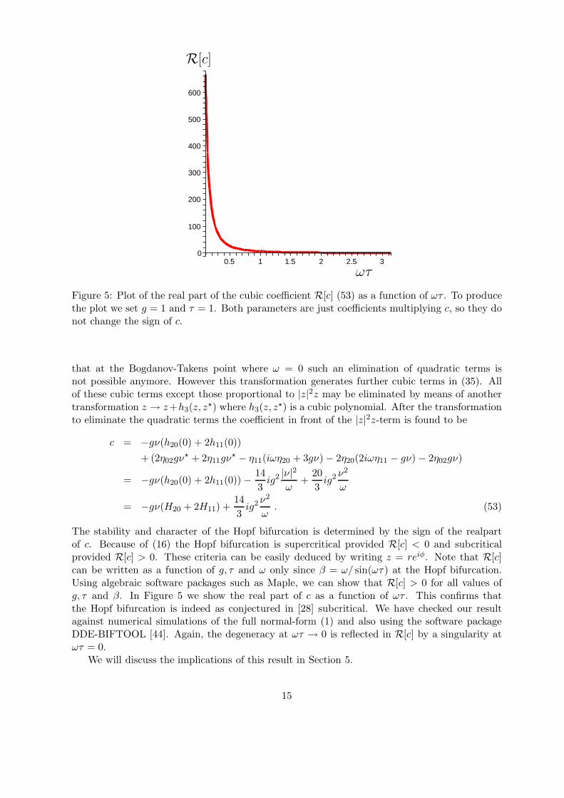
Figure 5: Plot of the real part of the cubic coefficient R[c] (53) as a function of ωτ . To producethe plot we set g = 1 and τ = 1. Both parameters are just coefficients multiplying c, so they donot change the sign of c.

that at the Bogdanov-Takens point where ω = 0 such an elimination of quadratic terms isnot possible anymore. However this transformation generates further cubic terms in (35). Allof these cubic terms except those proportional to |z|2z may be eliminated by means of anothertransformation z → z+h3(z, z⋆) where h3(z, z⋆) is a cubic polynomial. After the transformationto eliminate the quadratic terms the coefficient in front of the |z|2z-term is found to be

c = −gν(h20(0) + 2h11(0))

+ (2η02gν⋆ + 2η11gν⋆ − η11(iωη20 + 3gν) − 2η20(2iωη11 − gν) − 2η02gν)

= −gν(h20(0) + 2h11(0)) −14

3ig2 |ν|

2

ω+

20

3ig2 ν2

ω

= −gν(H20 + 2H11) +14

3ig2 ν2

ω. (53)

The stability and character of the Hopf bifurcation is determined by the sign of the realpartof c. Because of (16) the Hopf bifurcation is supercritical provided R[c] < 0 and subcriticalprovided R[c] > 0. These criteria can be easily deduced by writing z = reiφ. Note that R[c]can be written as a function of g, τ and ω only since β = ω/ sin(ωτ) at the Hopf bifurcation.Using algebraic software packages such as Maple, we can show that R[c] > 0 for all values ofg, τ and β. In Figure 5 we show the real part of c as a function of ωτ . This confirms thatthe Hopf bifurcation is indeed as conjectured in [28] subcritical. We have checked our resultagainst numerical simulations of the full normal-form (1) and also using the software packageDDE-BIFTOOL [44]. Again, the degeneracy at ωτ → 0 is reflected in R[c] by a singularity atωτ = 0.

We will discuss the implications of this result in Section 5.

15

-2

-1

0

1

2

sin(ω

τ),

ωτ/(

βτ)

ωτ0 π 2π 3π 4π

Figure 6: Illustration of the solutions and number of solutions of the implicit equation (54) forω. Green curve: βτ = 0.1, no Hopf bifurcation; light blue curve: βτ = 5, Hopf bifurcation withone marginal mode; dark blue curve: βτ = 143, Hopf bifurcation with finitely many marginalmodes; pink curve: βτ = ∞, Hopf bifurcation with infinitely many marginal modes.

4 The limit of large delay times: The Hopf bifurcation for wave

trains

In the previous Section we have described the Hopf bifurcation for small ωτ when there is onlyone marginal mode. This describes the behaviour of a single pulse on a ring. In this Sectionwe will pursue the case of large delay times when a pseudo-continuum of critical Hopf modesoccurs. We will derive a Ginzburg-Landau equation as an amplitude equation describing near-threshold behaviour of such a pseudo-continuum. The connection between amplitude equationsand delay-differential equations has long been known [45, 46, 47, 48, 49, 50]. The cross-overfrom a finite-dimensional center-manifold to an infinite-dimensional amplitude equation can bebest viewed when looking at the Hopf condition (7)

ω = β sin ωτ . (54)

For βτ > 7.789 there are at least two solutions of (54) for ω. This equation has arbitrary manysolutions ωk for βτ → ∞ and we obtain a pseudo-continuum in an interval with lower closedboundary at ωτ and upper boundary ωτ = π. At the singular limit ωτ = π there are countablyinfinitely many eigenvalues ωkτ = kπ. An illustration is given in Fig. 6. Note that the upperboundary ωτ = π corresponds to the coalescence of the Hopf bifurcation with the pitchforkbifurcation in the case of several pulses on a ring (see Section 2).

All these solutions are marginal and would have to be included in the ansatz (32). Note thatfor excitable media where β = β0 exp(−κτ) (see (2)) this limit cannot be achieved by simplyletting τ → ∞. The function βτ has a maximum at τ = 1/κ. So in order to have βτ → ∞one can either have β0 → ∞ which seems unphysical or κ → 0 with τ → ∞ to keep κτ finite.Hence the limit βτ → ∞ applies to media with a very slowly decaying inhibitor in a very largedomain. Large domain instabilities are known from certain excitable reaction diffusion systems

16

in the context of autocatalytic oxidation of CO to CO2 on platinum [51, 52, 53].

The case ωτ ≈ π is important for single pulses in a ring and for wave trains. Firstly, it describesthe case for a single pulse when a continuum of modes becomes unstable to a Hopf bifurcation.But more importantly it describes the case of a wave train with distinct members when thepitchfork bifurcation coalesces with the Hopf bifurcation. The point of coalescence is at µPF

given by (11) and with amplitude given by (12) which we recall

XPF =β

2g(1 − γ1) .

At this point of coalescence the Hopf frequency is in resonance with the spatial instability inwhich every second pulse dies. At µPF the two equations (3) describing the alternating modesin a wave train collapse to the single equation for one pulse (1) (see also Fig. 3). This Sectionwill investigate whether the coalescence of the subcritical pitchfork bifurcation with the Hopfbifurcation may produce stable oscillations.

We will perform a multiple scale analysis of the normal form (1) along the lines of [48]. We willobtain at third order an evolution equation for the amplitude as a solvability condition whichdescribes the dynamics close to the Hopf bifurcation. We consider the case of large delay timesτ and introduce a small parameter ǫ = 1/τ . To capture the dynamics close to the point ofcoalescence we introduce a slow time scale

s = ǫt ,

and rewrite the normal form (1) in terms of the slow variable as

ǫ∂sX = −µ − gX2 − β(γ + X(s − 1) + γ1X) . (55)

We expand the scalar field X(s) as

X = xPF + ǫx1 + ǫ2x2 + ǫ3x3 + · · · .

Using the generic scaling the bifurcation parameter can be written as

µ = µPF + ǫ2∆µ + · · · .

A Taylor expansion of (54) around ωτ = π yields at first order ωτ = βτ(π −ωτ) which for largeτ (small ǫ) we may write as

ωτ = π(1 −1

βτ+

1

(βτ)2) = π(1 −

1

βǫ +

1

β2ǫ2) . (56)

This suggests a multiple time scaling

∂s = ∂s0+ ǫ∂s1

+ ǫ2∂s2+ · · · .

Close to the bifurcation point critical slowing down occurs which allows us to expand the delayterm for large delays as

X(s − 1) = e−∂sX(s) (57)

≈

[

1 − ǫ∂s1+ ǫ2

(

1

2∂s1s1

− ∂s2

)]

e−∂s0X(s) . (58)

17

At lowest order, O(1), we obtain the equation determining xPF . At the next order we obtain

Lx1 = 0 , (59)

with the linear operator

L = β[

1 + e−∂s0

]

.

Equation (59) is solved by

x1(s0, s1, s2) = z(s1, s2)eiπs0 + z(s1, s2)e

−iπs0 , (60)

with complex amplitude z and its complex conjugate z. Note that on the fast time scale t wewould have x1(t) = z exp(iωt) + c.c. with ωτ = π, which, of course, is the Hopf mode at onset.

At the next order, O(ǫ2), we obtain

Lx2 = −∆µ − gx21 − ∂s0

x1 + β∂s1e−∂s0x1 . (61)

The right-hand side involves terms proportional to exp(±iπs0), which are resonant with thehomogeneous solution of Lx2 = 0. We therefore impose the solvability condition

∂s0x1 − β∂s1

e−∂s0x1 = 0 ,

which using (59) reads as

∂s1x1 +

1

β∂s0

x1 = 0 . (62)

In terms of the complex amplitude z using (60) this reads as

∂s1z +

1

βiπz = 0 . (63)

This amounts to the time scale iωτ ≈ τ∂t ≈ ∂s0+ ǫ∂s1

= iπ − iǫπ/β = iπ(1 − 1/(βτ)) whichcorresponds to our scaling (56) at first order. Provided (63) is satisfied we can readily solve (61)by solving for each appearing harmonic, and find

x2 = −1

2β

[

∆µ + 2g|z|2 + gz2e2iπs0 + gz2e−2iπs0

]

= −1

2β

[

∆µ + gx21

]

, (64)

where we used (59).At the next order, O(ǫ3), we obtain the desired evolution equation as a solvability condition. AtO(ǫ3) we obtain

Lx3 = −∂s0x2 + β∂s1

e−∂s0 x2 − ∂s1x1 − 2gx1x2 −

1

2β∂s1s1

e−∂s0x1 + β∂s2e−∂s0 x1

= −∂s0x2 + β∂s1

e−∂s0 x2 − ∂s1x1 − 2gx1x2 +

1

2β∂s1s1

x1 − β∂s2x1 . (65)

18

Again resonant terms proportional to exp(±iπs0) are eliminated by imposing a solvability con-dition which upon using the expressions for x2 yields the desired amplitude equation

∂s2x1 −

1

β2∂s0

x1 =g

β2∆µ x1 +

1

2β2∂s0s0

x1 +g2

β2x3

1 . (66)

This is the well-studied real Ginzburg-Landau equation [54]. The time-like variable is the slowtime scale s2 and the space-like variable the faster time scale s0 which is O(τ). As in the finitedimensional case studied in Section 3 the Hopf bifurcation is clearly subcritical since the realpart of the coefficient in front of the cubic term in (66) is positive for all parameter values. Hencethe coalescence of the Hopf bifurcation and the pitchfork bifurcation cannot lead to stable os-cillations. We have shown that wave trains also undergo unstable oscillations in the frameworkof the normal form (1).

The usefulness of the spatio-temporal view point for delay differential equations as expressedhere in the Ginzburg-Landau equation (66) has been pointed out [45, 46, 48, 50]. However theGinzburg-Landau equation (66) may be cast into a finite dimensional system which emphasizesthe underlying multiple scale analysis. We start by rewriting (66) as an equation for the complexamplitude z. One can explicitly express s0-derivatives and obtain the following finite dimensionalsystem

∂s2z − iπ

1

β2z =

g

β2

(

∆µ −π2

2g

)

z + 3g2

β2|z|2z . (67)

The time-scaling on the left hand-side is as expected from our initial linearization and expansionof the frequency (56). We have in total

iωτ ≈ τ∂t = ∂s ≈ ∂s0+ ǫ∂s1

+ ǫ2∂s2= iπ

(

1 −1

βτ+

1

(βτ)2

)

,

which corresponds to (56). This illustrates the multiple-scale character of our analysis wherethe nonlinear term may be interpreted as a frequency correction [55]. The correction term tothe linear term on the right-hand side of (67) shows that the onset is retarded on the very slowtime scale s2.

In [21] a real Ginzburg-Landau equation was derived for paced excitable media with an addi-tional integral term modeling the pacing. It would be interesting to see whether the thereinderived amplitude equation can be derived in a multiple scale analysis along the lines of thismultiple scale analysis.

5 Summary and Discussion

We have explored the Hopf bifurcations of a single pulse and of a wave train in a ring of excitablemedium. We have found that for the phenomenological normal form (1) the Hopf bifurcationfor a single pulse on a ring and for a wave train on a ring is always subcritical independent onthe equation parameters.

19

Hopf bifurcations in excitable media had been previously studied. Besides numerical investi-gations of the Barkley model [33], the modified Barkley model [34], the Beeler-Reuter model[56, 57, 11, 29, 30, 58], the Noble-model [59, 17, 29] and the Karma-model [17], where a Hopfbifurcation has been reported, there have been many theoretical attempts to quantify this bi-furcation for a single-pulse on a ring. Interest has risen recently in the Hopf bifurcation in thecontext of cardiac dynamics because it is believed to be a precursor of propagation failure ofpulses on a ring. The Hopf bifurcation has been related to a phenomenon in cardiac excitablemedia which goes under the name of alternans. Alternans describe the scenario whereby actionpotential durations are alternating periodically between short and long periods. The interestin alternans has risen as they are believed to trigger spiral wave breakup in cardiac tissue andventricular fibrillation [15, 11, 17, 16, 18].

Our results may shed a new light on what may be called alternans. The occurrence of alter-nans in clinical situations is often followed by spiral wave breakup and ventricular fibrillation[15, 11, 16, 17, 18]. The subcritical character of the Hopf bifurcation gives a simple and straight-forward explanation for this phenomenon. Moreover, if the system length L is slowly varied,long transients may be observed of apparently stable oscillations (see Figure 7 and Figure 8).Depending on whether the system length is below or above the critical length LH the oscillationswill relax towards the homogeneous state or the instability will lead to wave breakup. However,even for the case of relaxation towards the stable homogeneous solution, these oscillations maylead to wave breakup upon further reduction of the system length, because of the subcriticalcharacter of the Hopf bifurcations. This illustrates the diagnostic importance of cardiac alter-nans.

5.1 Limitations and range of validity of our results

Strictly speaking, our result that the Hopf bifurcation is subcritical for the normal form (1)cannot be taken as a prove that alternans are unstable for all excitable media. The normal form(1) is only valid for a certain class of excitable media. In particular it describes the situation inwhich an activator weakly interacts with the inhibitor of the preceding exponentially decayinginhibitor. Moreover, the normal form has only been phenomenologically derived in [28]. Ofcourse, unless a rigorous derivation of the normal form (1) has been provided the results pre-sented here may serve as nothing more than a guidance in interpreting alternans in real cardiacsystems or more complex ionic models of excitable media, and may alert scientists to checkresults on stability of oscillations more carefully.

Several simplifications have been made to obtain the normal form (1) in [28]. For example, thetime delay τ = L/c0 is treated as constant. This is obviously not correct for Hopf bifurcations.However, the inclusion of γ1 (which is essential in the quantitative description of the Hopf bi-furcation) allows for velocity dependent effects. Guided by the success of the normal form toquantitatively describe a certain class of excitable media and by numerical experiments we arehopeful that our result may help interpreting experiments and numerical simulations.

In Section 5.3 we will discuss a particular model for cardiac dynamics in which for certain pa-rameter values the assumptions for the derivation of our normal form are violated. For theseparameter values stable oscillations may occur. However even for systems which are described

20

by the normal form (1) a word of caution is appropriate. If the oscillatory solutions bifurcatingfrom the stationary solution are unstable as we have proven here, the unstable Hopf branch couldin principle fold back and restabilize. Our analysis does not include such secondary bifurcations.Another scenario which we cannot exclude based on our analysis is that the unstable branchmay be a basin of attraction for a stable oscillatory solution far away from the homogeneoussolution. However, our numerical simulations do not hint towards such scenarios.From an observational perspective the relevance of the subcritical instability for spiral wavebreakup is a matter of the time scale of the instability. The time scale associated with thesubcritical Hopf bifurcation may be very long as seen in Fig. 9. This time scale becomes shorterthe further the perturbation in the bifurcation parameter is from its value at the correspondingstable stationary pulse solution. In any case, if the parameter is kept fixed above the criticalvalue, the instability will eventually develop unless the life time of a reentrant spiral is less thanthe time scale of the instability. For clinical applications one would need to estimate the timescale of a reentrant spiral and compare it with the time scale of the instability. Such estimateshowever are not meaningful for simple models such as the Barkley model.

Our definition of alternans is restricted to non-paced pulses on a ring. If the excitable media ispaced, the subcritical character of the Hopf bifurcation is not guaranteed anymore, and thereis no a priori reason why stable alternans cannot occur. Indeed, in periodically stimulatedexcitable media stable alternans have been reported [60, 61, 19, 20, 21, 23, 24]. A non-pacedsingle pulse on a ring is a simple model for a reentrant spiral moving around an anatomicalobstacle or around a region of partially or totally inexcitable tissue. As such it ignores thedynamics of the spiral away from the obstacle. An extension would be to look at a transversalone-dimensional slice through a spiral and consider wave trains and instabilities of such wavetrains.

5.2 Relation to the restitution condition

Since the pioneering work [12] alternans have been related to a period-doubling bifurcation.This work has rediscovered the results by [15], which had hardly been noticed by the scientificcommunity until then. In there it was proposed that the bifurcation can be described by aone-dimensional return map relating the action potential duration (APD) to the previous re-covery time, or diastolic interval (DI), which is the time between the end of a pulse to the nextexcitation. A period-doubling bifurcation was found if the slope of the so called restitution curvewhich relates the APD to the DI, exceeds one. A critical account on the predictive nature ofthe restitution curve for period-doubling bifurcations is given in [62, 23]. In [29] the instabilitywas analyzed by reducing the partial differential equation describing the excitable media to adiscrete map via a reduction to a free-boundary problem. In [34] the Hopf bifurcation couldbe described by means of a reduced set of ordinary-differential equations using a collective co-ordinate approach. In [11, 30, 58, 26] the bifurcation was linked to an instability of a singleintegro-delay equation. The condition for instability given by this approach states - as in someprevious studies involving one-dimensional return maps - that the slope of the restitution curveneeds to be greater than one. However, as evidenced in experiments [63, 64] and in theoreticalstudies [62, 23, 65, 66, 67] alternans do not necessarily occur when the slope of the restitutioncurve is greater than one. In our work we have a different criterion for alternans (which weinterpret now as unstable periodic oscillations). Our necessary condition for the occurrence ofalternans, βτ > 1, does not involve the restitution curve but involves the coupling strength and

21

the wave length. Moreover, in Fig. 4(b) we can see that for our normal form pulses can be stablefor values of βτ ≫ 1 in accordance with the above mentioned experiments and numerical studies.

In the following we will show how our necessary condition for the onset of instability βτ > 1can be related to the restitution condition, that the onset of instability is given when the slopeof the restitution curve exceeds 1.

Close to the saddle node the Hopf frequency is ωτ ≈ 0. We introduce a small parameter δ ≪ 1and write close at the saddle node

X = XSN + δx ,

where XSN is given by (5). The generic scaling close to the saddle node implies that we maywrite µ = µSN + δ2∆µ. Using the critical slowing down at the saddle node and the fact thatωτ ≈ 0 we may approximate the normal form (1) to describe the temporal change of X at sometime t and at some later time t + τ .

δxn+1 − δxn

τ= −µSN − δ2∆µ − g(XSN + δxn)2 − β(γ + XSN + γ1XSN + δxn−1 + γ1δxn) .

Here xn = x(tn) and xn+1 = x(tn + τ). Neglecting terms of O(δ2) and using the definition ofthe saddle node (5) we end up with

xn+1 − (1 + βτ)xn + βτxn−1 = 0 .

This equation has either the solution xn = 1 which corresponds to the stable steady solutiondescribed by X1 of (4), or

xn = (βτ)nx0 ,

which implies the map

xn = βτxn−1 . (68)

Close to the saddle node the amplitude of the activator xn correlates well with the APD, and wefind that βτ > 1 is exactly the restitution condition whereby the slope of the restitution curvehas to be larger than one.

Our model contains the restitution condition as a limiting case when the Hopf bifurcation occursclose to the saddle node. However, as seen in Fig. 4 βτ may be larger than one but still thesystem supports stable pulses. These corrections to the restitution conditions are captured byour model. Moreover, the normal form is able to determine the frequency at onset.

We note that the parameter γ1 does not enter the restitution condition; it is not needed for theexistence of a Hopf bifurcation (cf. (7) and (8)). However, as pointed out in [28] quantitativeagreement with numerical simulations is only given if γ1 is included. In [28] the inclusion of theγ1-term takes into account the velocity dependent modifications of the bifurcation behaviour:large-amplitude pulses have a higher velocity than low-amplitude ones. A larger pulse will there-fore run further into the inhibitor generated by its predecessor. Velocity restitution curves havebeen studied in [65] to allow for a modification of the restitution condition derived in [30] for a

22

single pulse in a ring. The normal form incorporates naturally these velocity dependent terms.

For a recent numerical study on the validity of the restitution condition the reader is referred to[67]. In this work the stability of certain excitable media is investigated by means of numericalcontinuation methods which allows a precise identification of the onset of oscillations. At theonset of alternans the restitution curve was determined. It was found that the restitution con-dition failed for three out of four cases for pulses in a one-dimensional ring. Our result suggeststhat the restitution condition may be a good indicator for the onset of alternans close to thesaddle node.

5.3 Numerical simulations

In the context of alternans the Hopf bifurcation had been described as a supercritical bifurcation[11, 17, 29, 30] and not as we have found here as a subcritical bifurcation (although at the sametime their occurrence had been related to wave breakup [29]). We therefore revisit some of theprevious numerical studies. In [17] the following two-variable model was proposed

ǫ∂tE = ǫ2∂xxE − E +

[

A −

(

n

nB

)M]

(1 − tanh(E − 3))E2

2

∂tn = θ(E − 1) − n , (69)

as a model for action potential propagation in cardiac tissue. Here θ(x) is the Heaviside stepfunction. This model incorporates essential features of electrophysiological cardiac models. Forthe parameters A = 1.5415, ǫ = 0.009, M = 30 and nB = 0.525 a supercritical Hopf bifurcationwas reported upon diminishing the system length L. We integrate this model using a pseu-dospectral Crank-Nicolson method where the nonlinearity is treated with an Adams-Bashforthscheme. We use a timestep of dt = 0.00001 and 4096 spatial grid points. A Hopf bifurcationoccurs around L = 0.215. To approach the Hopf bifurcation we created a stable pulse for somelarge system length, and subsequently diminished the system length L. In Figure 7 we show thatfor these parameters the bifurcation is actually subcritical. The subcritical character has notbeen recognized before - probably because of insufficiently short integration times. For systemlength L just above the critical length the oscillations can appear stable for a very long time(see Figure 8) before they settle down to the homogeneous solution.

Indeed, as already stated in our paper [28], the number of oscillations may be rather largewhen the instability is weak. In Figure 9 we show such a case for the maximal amplitude of theactivator u for the modified Barkley model

∂tu = D∂xxu + u(1 − u)(u − us − v)

∂tv = ǫ (u − a v) , (70)

which is a reparameterized version of a model introduced by Barkley [32]. It is clearly seen thatthe oscillations can appear stable for a very long time and many oscillations (in this case morethan 500 oscillations) which has lead scientists to the false conclusion that the Hopf bifurcationis supercritical.

The normal forms (1) or (3) were derived for situations in which the activator weakly interactswith the tail of the preceding inhibitor which exponentially decays towards the homogeneous rest

23

0

1

2

3

4

0 10 20 30 40 50 60 70

E

t

2.5

3

3.5

4

0 5 10 15 20 25

E

t

Figure 7: Temporal behaviour of the maximal amplitude Emax of the activator E for model (69)just above the subcritical Hopf bifurcation. The parameters are A = 1.5415, ǫ = 0.009, M = 30and nB = 0.525 and L = 0.215. The inlet shows the behaviour at L = 0.210.

3.61

3.62

3.63

3.64

0 5 10

E

t

3.61

3.62

3.63

3.64

0 50 100 150 200

E

t

Figure 8: Temporal behaviour of the maximal amplitude Emax of the activator E for model (69).The system length is just below the Hopf bifurcation with L = 0.22; the other parameters are asin Figure 7. (a): The oscillations appear to be stable over some time. (b): Same parameters as in(a) but longer integration time. The apparent stability has to be accounted for by insufficientlylong integration times. The solution adjusts to the homogeneous solution. Note the long timescales which contain hundreds of oscillations.

24

0.835

0.84

0 4000 8000 12000 16000

u

t

Figure 9: Temporal behaviour of the maximal amplitude umax of the activator u for model (70)just above the subcritical Hopf bifurcation. The parameters are a = 0.22, us = 0.1, ǫ = 0.03755and L = 246. The oscillations appear stable for a very long time but will eventually either dampout and attain a constant non-zero value in the case, when L is larger than the critical LH atwhich the Hopf bifurcation occurs, or in the case L < LH the pulse will collapse as depicted inFigure 7 confirming the subcritical character of the Hopf bifurcation.

state. Then one can describe the influence of the tail of the preceding inhibitor as a perturbationto the generic saddle node of the isolated pulse. The models discussed so far all fall into thiscategory. A different model was introduced by Echebarria and Karma in [21] which as we willsee below for certain parameter regions does not fall into this class of model but supports stableoscillations. Originally the model was studied for a paced strand but recently has also beenstudied in a ring geometry [68]. It has been argued in [68] in the framework of amplitudeequations that the nature of the bifurcation for the ring dynamics, whether supercritical orsubcritical, is determined by the action potential duration restitution curve for a propagatedpulse. In the following we study numerically the Hopf bifurcation for this model in a ringgeometry. This will illustrate the range of validity for our normal form and the conclusionswhich may be drawn with respect to the stability of cardiac alternans. The model consists ofthe standard cable equation

∂tV = D∂xxV −Iion

Cm, (71)

where Iion models the membrane current and Cm is the capacity of the membrane. In [21] thefollowing form for the membrane current was proposed

Iion

Cm

=1

τ0

(

S + (1 − S)V

Vc

)

−1

τa

hS , (72)

with a switch function

S =1

2

(

1 + tanh(V − Vc

ǫ)

)

. (73)

The gate variable h evolves according to

dh

dt=

1 − S − h

τm(1 − S) + τpS. (74)

25

0

0.05

0.1

0.15

0 10000 20000 30000

0.16335

0.16355

0.16375

2000 4000 6000

V

V

t

t

Figure 10: Temporal behaviour of the maximal amplitude Vmax of the activator V for model(71)-(74). The parameters are τ0 = 150, τa = 26, τm = 60, τp = 12, Vc = 0.1, D = 0.00025and ǫ = 0.005. The main figure is obtained for L = 1.11 which is slightly above the subcriticalHopf bifurcation confirming the subcritical character of the Hopf bifurcation. The inset is forL = 1.1175 which is slightly below the bifurcation point.

0X

time

Figure 11: Space-time plot of stable oscillations occurring at τa = 6 with L = 4.8 for the model(71)-(74). The other parameters are as in Fig. 10. Stable oscillations are found for a range ofring lengths L.

The stable homogeneous rest state is at V = 0 and h = 1; however for small τa a second sta-ble focus may arise. For details on the physiological interpretations of the model the reader isreferred to [21, 68]. For the numerical integration we use again a semi-implicit pseudospectralCrank-Nicolson method where the nonlinearity is treated with an Adams-Bashforth scheme. Weuse a timestep of dt = 0.01 and 1024 spatial grid points. In Fig. 10 we show an example for asubcritical Hopf bifurcation in this model consistent with our theory. However, for sufficientlysmall τa a supercritical Hopf bifurcation arises upon decreasing the ring length L. In Fig. 11we present a space-time plot for such a situation of stable oscillations. Whereas the subcriticalcase is consistent with our theory we now have to understand why for small τa stable oscillationsoccur. In order to do so it is helpful to look at the spatial profiles of the activator and the in-hibitor close to the Hopf bifurcation which are presented in Fig. 12. In the left figure we see theactivator V and the inhibitor 1−h for the case of a subcritical Hopf bifurcation as seen in Fig. 10.The figure is similar to Fig. 1 for the modified Barkley model. The activator weakly interacts

26

0

0.5

1

0 0.25 0.5 0.75 1

V , h

x 0

0.5

1

0 1 2 3 4

V , h

x

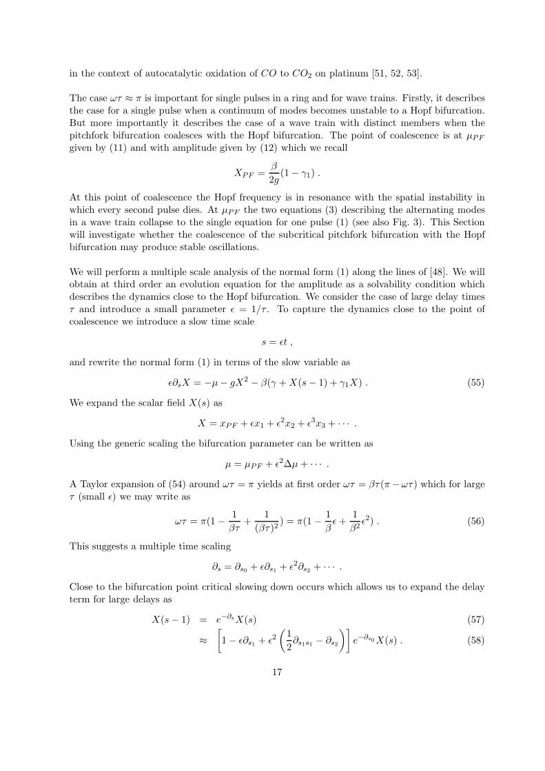
Figure 12: Plot of the activator V (continuous line) and the inhibitor h (dashed line) for thesystem (71)-(74). We plot here 1 − h rather than h to have the homogeneous rest state atu = 0 and 1 − h = 0. Parameters are τ0 = 150, τm = 60, τp = 12, Vc = 0.1, D = 0.00025 andǫ = 0.005. Left: The activator runs into the exponentially decaying tail of the inhibitor whichdecays towards the rest state 1 − h = 0. This is similar to the behaviour in Fig. 1. Parametersare τa = 26 with L = 1.11. This scenario is well described by the normal form. Right: Theactivator does not interact with the exponentially decaying tail corresponding to the rest statebut rather with the metastable state defined by h = 0. Parameters are τa = 6 with L = 4.8.This case cannot be captured by the normal form.

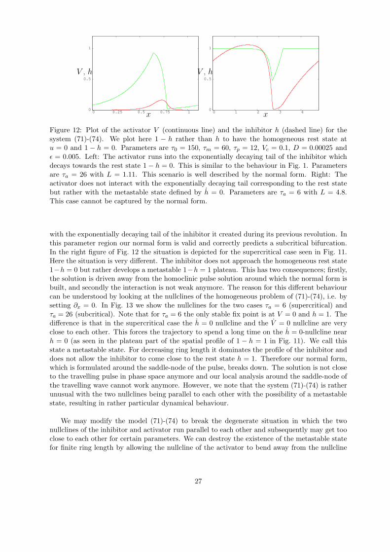
with the exponentially decaying tail of the inhibitor it created during its previous revolution. Inthis parameter region our normal form is valid and correctly predicts a subcritical bifurcation.In the right figure of Fig. 12 the situation is depicted for the supercritical case seen in Fig. 11.Here the situation is very different. The inhibitor does not approach the homogeneous rest state1−h = 0 but rather develops a metastable 1−h = 1 plateau. This has two consequences; firstly,the solution is driven away from the homoclinic pulse solution around which the normal form isbuilt, and secondly the interaction is not weak anymore. The reason for this different behaviourcan be understood by looking at the nullclines of the homogeneous problem of (71)-(74), i.e. bysetting ∂x = 0. In Fig. 13 we show the nullclines for the two cases τa = 6 (supercritical) andτa = 26 (subcritical). Note that for τa = 6 the only stable fix point is at V = 0 and h = 1. Thedifference is that in the supercritical case the h = 0 nullcline and the V = 0 nullcline are veryclose to each other. This forces the trajectory to spend a long time on the h = 0-nullcline nearh = 0 (as seen in the plateau part of the spatial profile of 1 − h = 1 in Fig. 11). We call thisstate a metastable state. For decreasing ring length it dominates the profile of the inhibitor anddoes not allow the inhibitor to come close to the rest state h = 1. Therefore our normal form,which is formulated around the saddle-node of the pulse, breaks down. The solution is not closeto the travelling pulse in phase space anymore and our local analysis around the saddle-node ofthe travelling wave cannot work anymore. However, we note that the system (71)-(74) is ratherunusual with the two nullclines being parallel to each other with the possibility of a metastablestate, resulting in rather particular dynamical behaviour.

We may modify the model (71)-(74) to break the degenerate situation in which the twonullclines of the inhibitor and activator run parallel to each other and subsequently may get tooclose to each other for certain parameters. We can destroy the existence of the metastable statefor finite ring length by allowing the nullcline of the activator to bend away from the nullcline

27

0 0.05 0.1 0.15 0.20

0.5

1

V

h

0 0.05 0.1 0.15 0.20

0.5

1

V

h

0 0.05 0.1 0.15 0.20

0.5

1

V

h

Figure 13: Nullclines for the system (71)-(74). The dark lines denote the V = 0 nullclines andthe grey lines the h = 0 nullclines. Parameters are τ0 = 150, τm = 60, τp = 12, Vc = 0.1 andǫ = 0.005, and for all cases only one stable fix point exists at V = 0 and h = 1. Left: Thesubcritical case with τa = 26. Middle: The supercritical case with τa = 6. Note the closenessof the nullclines for large V . Right: Nullclines for the modified equation (75) which breaks thenear degeneracy of the nullclines observed in the middle figure. Here τa = 6 and τl = 3.

of the inhibitor if we, for example, consider the following modification of the membrane current

Iion

Cm

=1

τ0

(

S + (1 − S)V

Vc

)

+1

τl

V 2 −1

τa

hS , (75)

with some sufficiently small τl. Then we are again in the situation where the rest state V = 0 andh = 1 dominates the dynamics upon decreasing the ring length L. The nullclines are shown inFig. 13. We confirmed that for τl = 3 the Hopf bifurcation is indeed subcritical, consistent withour theoretical result. We note that the actual value of τl is not important for the existence ofsubcritical bifurcation but rather that a sufficiently small τl breaks the geometric structure of thedegenerate nullclines and allows the activator nullcline to bend away from the inhibitor nullcline.The model (71)-(74) illustrates for which class of excitable media our normal form is applicableand for which systems we may draw conclusions on the stability of dynamical alternans in a ring.

Acknowledgements I would like to thank Sebastian Hermann for helping with the DDE-BIFTOOL software, and Martin Wechselberger for fruitful discussions. I gratefully acknowledgesupport by the Australian Research Council, DP0452147 and DP0667065.

References

[1] A.T. Winfree, When Time Breaks Down (Princeton University Press, 1987).

[2] J.M. Davidenko, A.M. Pertsov, R. Salomonsz, W. Baxter and J. Jalife, Stationary and

drifting spiral waves of excitation in isolated cardiac muscle, Nature 335, 349–351 (1992).

[3] F. Siegert and C. Weijer, Analysis of optical density wave propagation and cell movement

in the cellular slime mold dictyostelium discoideum, Physica 49D, 224–232 (1991).

[4] M. D. Berridge, P. Lipp and M. J. Bootman, The versality and universality of calcium

signalling, Nature Reviews Molecular Cell Biology 1, 11–21 (2000).

28

[5] A. T. Winfree, Spiral Waves of Chemical Activity, Science 175, 634–636 (1972).

[6] A. T. Winfree, Stable particle-like solutions to the nonlinear wave equations of the three-

dimensional excitable media, SIAM. Rev. 32, 1–53 (1990).

[7] A. T. Winfree, Electrical Turbulence in Three-Dimensional Heart Muscle, Science 266,1003–1006 (1994).

[8] D. Margerit and D. Barkley, Selection of twisted scroll waves in three-dimensional excitable

media, Phys. Rev. Lett. 86, 175–178 (2001).

[9] D. Margerit and D. Barkley, Cookbook asymptotics for spiral and scroll waves in excitable

media, Chaos 12, 636–649 (2002).

[10] see review articles in the focus issue Chaos 8, 1 (1998).

[11] M. Courtemanche, L. Glass and J. P. Keener, Instabilities of a propagating pulse in a ring

of excitable media, Phys. Rev. Lett. 70, 2182–2185 (1993).

[12] M. R. Guevara, G. Ward, A. Shrier and L. Glass, Electrical alternans and period-doubling

bifurcations, In: ”IEEE Computers in Cardiology”, IEEE Computer Society, Silver Spring,167–170 (1984).

[13] G. R. Mines, On circulating excitations in heart muscles and their possible relation to

tachycardia and fibrillation, Trans. Roy. Soc. Can. 4, 43–53 (1914).

[14] L. H. Frame and M. B. Simson, Oscillations of conduction, action potential duration, and

refractoriness, Circulation 78, 1277–1287 (1988).

[15] J.B. Nolasco and R.W. Dahlen, A graphic method for the study of alternation in cardiac

action potentials, J. Appl. Physiol. 25, 191–196 (1968).

[16] A. Karma, Electrical alternans and spiral wave breakup in cardiac tissue, Chaos 4, 461–472(1994).

[17] A. Karma, Spiral breakup in model equations of action potential propagation in cardiac

tissue, Phys. Rev. Lett. 71, 1103–1106 (1993).

[18] F. H. Fenton, E. M. Cherry, H. M. Hastings and S. J. Evans, Multiple mechanisms of spiral

wave breakup in a model of cardiac electrical activity, Chaos 12, 852–891 (2002).

[19] H. M. Hastings, F. H. Fenton, S. J. Evans, O. Hotomaroglu, J. Geetha, K. Gittelson,J. Nilson and A. Garfinkel, Alternans and the onset of ventricular fibrillation, Phys. Rev. E62, 4043–4048 (2000).

[20] H. Arce, A. Lopez and M. R. Guevara, Triggered alternans in an ionic model of ischemic

cardiac ventricular muscle, Chaos 12, 807–818 (2002).

[21] B. Echebarria and A. Karma, Instability and spatiotemporal dynamics of alternans in paced

cardiac dynamics, Phys. Rev. Lett. 88, 208101-1–208101-4 (2002).

[22] B. Echebarria and A. Karma, Spatiotemporal control of cardiac alternans, Chaos 12, 923–930 (2002).

29

[23] J. J. Fox, E. Bodenschatz and R. F. Gilmour, Period-doubling instability and memory in

cardiac tissue, Phys. Rev. Lett. 89, 1381011–1381014 (2002).

[24] H. Henry and W. -J. Rappel, Dynamics of conduction blocks in a model of paced cardiac

tissue, Phys. Rev. E 71, 051911-1–051911-7 (2005).

[25] A. Vinet, Memory and bistability in a one-dimensional loop of model cardiac cells,J. Syst. Biol. 7, 451–473 (1999).

[26] P. Comtois and A. Vinet, Stability and bifurcation in an integral-delay model of cardiac

reentry including spatial coupling in repolarization, Phys. Rev. E 68, 051903 (2003).

[27] P. Comtois and A. Vinet, Multistability of reentrant rhythms in an ionic model of a two-

dimensional annulus of cardiac tissue, Phys. Rev. E 72, 051927 (2005).

[28] G. A. Gottwald and L. Kramer, A normal form for excitable media, Chaos 16, 013122(2006).

[29] A. Karma, H. Levine and X. Zou, Theory of pulse instabilities in electrophysiological models

of excitable tissues, Physica D 73, 113–127 (1994).

[30] M. Courtemanche, L. Glass and J. P. Keener, A delay equation representation of pulse

circulation on a ring in excitable media, SIAM J. Appl. Math. 56, 119–142 (1996).

[31] R. FitzHugh, Impulses and physiological states in theoretical models of nerve membranes,Biophys. J. 1, 445–466 (1961); J. Nagumo, S. Arimoto and S. Yoshizawa, An active pulse

transmission line simulating 1214-nerve axons, Proc. IRE 50, 2061–2070 (1962).

[32] D. Barkley, A model for fast computer simulation of waves in excitable media, Physica 49D,61–70 (1991).

[33] M. Knees, L. S. Tuckerman and D. Barkley, Symmetry-breaking bifurcations in one-

dimensional excitable media, Phys. Rev. A 46, 5054–5062 (1992).

[34] G. A. Gottwald and L. Kramer, On propagation failure in 1 and 2 dimensional excitable

media, Chaos 14, 855–863 (2004).

[35] N. Krasovskii, Stability of motion, Stanford University Press (1963).

[36] J. K. Hale, Theory of Functional Differential Equations, Springer-Verlag, New-York, (1977).

[37] J. K. Hale and S. M. Verduyn Lunel, Introduction to Functional Differential Equations,Springer-Verlag, New-York, (1993).

[38] O. Diekmann, S. A. van Gils, S. M. Verduyn Lunel and H. O. Walther, Delay equations,Appl. Math. Sci. 110, Springer-Verlag, New-York, (1995).

[39] W. Wischert, A. Wunderlin, A. Pelster, M. Olivier and J. Groslambert, Delay-induced

instabilities in nonlinear feedback systems, Phys. Rev. E 49, 203–219 (1994).

[40] B. F. Redmond, V. G. LeBlanc and A. Longtin, Bifurcation analysis of a class of first-order

nonlinear delay-differential equations with reflectional symmetry, Physica D 166, 131–146(2002).

30

[41] J. Sieber and B. Krauskopf, Bifurcation analysis of an inverted pendulum with delayed

feedback control near a triple-zero eigenvalue singularity, Nonlinearity 17, 85–103 (2004).

[42] J. Carr, Application of the center manifold theory, volume 35 of Applied Math. Sci. Springer-Verlag, (1981).

[43] S. Wiggins, Introduction to Applied Nonlinear Dynamical Systems and Chaos, Springer–Verlag, New York, (1990)

[44] K. Engelborghs, T. Luzyanina and G. Samaey, DDE-BIFTOOL v. 2.00 user manual: a

Matlab package for bifurcation analysis of delay differential equations, Technical ReportTW-330, Department of Computer Science, K. U. Leuven, Leuven, Belgium, 2001.

[45] G. Giacomelli and A. Politi, Relationship between delayed and spatially extended dynamical

systems Phys. Rev. Lett. 76, 2686–2689 (1996).

[46] G. Giacomelli and A. Politi, Multiple scale analysis of delayed dynamical systems, PhysicaD 117, 26–42 (1998).

[47] M. Schanz and A. Pelster, Analytical and numerical investigations of the phase-locked loop

with time delay, Phys. Rev. E 67, 056205 (2003).

[48] M. Nizette, Front dynamics in a delayed-feedback system with external forcing, Physica D183, 220–244 (2003).

[49] A. Amann, E. Scholl and W. Just, Some basic remarks on eigenmode expansions of time-

delay dynamics, Physica A 373, 191–202 (2006).

[50] M. Wolfrum and S. Yanchuk, Eckhaus instability in systems with large delay,Phys. Rev. Lett. 96, 220201 (2006).

[51] M. G. Zimmermann, S. O. Firle, M. A. Natiello, M. Hildebrand, M. Eiswirth, M. Bar,A. K. Bangia and I. G. Kevrekidis, Pulse bifurcation and transition to spatiotemporal chaos

in an excitable reaction-diffusion model, Physica D 110, 92–104 (1997).

[52] J. Krishnan, I. G. Kevrekidis, M. Or-Guil, M. G. Zimmermann and M. Bar, Numerical

bifurcation and stability analysis of solitary pulses in an excitable reaction-diffusion model,Comput. Methods Appl. Eng. 170, 253–275 (1999).

[53] M. Or-Guil, J. Krishnan, I. G. Kevrekidis and M. Bar, Pulse bifurcations and instabilities

in an excitable medium: Computations in finite ring domains. Phys. Rev. E 64, 046212(2001).

[54] I. S. Aranson and L. Kramer, The world of the Complex Ginzburg-Landau Equation,Rev. Mod. Phys. 74, 99–143 (2002).

[55] F. Verhulst, Nonlinear Differential Equations and Dynamical Systems, Springer-Verlag,New York, (2000).

[56] G. W. Beeler and H. Reuter, Reconstruction of the action potential of ventricular myocardial

fibers, J. Physiol. 268, 177–210 (1977).

31

[57] W. Quan and Y. Rudy, Unidirectional block and reentry of cardiac excitation: a model

study, Circ. Res. 66, 367–382 (1990).

[58] A. Vinet, Quasiperiodic circus movement in a loop model of cardiac tissue: Multistability

and low dimensional equivalence, Ann. Biomed. Eng. 28, 704–720 (2000).

[59] D. Noble, A modification of the Hodgkin-Huxley equations applicable to Purkinje fibre action

and pacemaker potentials, J. Physiol. 160, 317–352 (1962).

[60] M. R. Guevara, L. Glass and A. Shrier, Phase locking, period-doubling bifurcations, and

irregular dynamics in periodically stimulated cardiac cells, Science 214, 1350–1353 (1981).

[61] T. J. Lewis and M. R. Guevara, Chaotic dynamics in an ionic model of the propagated

cardiac action potential, J. Theor. Biol. 146, 407–432 (1990).

[62] F. H. Fenton, S. J. Evans and H. M. Hastings, Memory in an excitable medium: a mech-

anism for spiral wave breakup in the low-excitability limit, Phys. Rev. Lett. 83, 3964–3967(1999).

[63] G. M. Hall, S. Bahar and D. J. Gauthier, Prevalence of Rate-Dependent Behaviors in

Cardiac Muscle, Phys. Rev. Lett. 82, 2995–2998 (1999).

[64] I. Banville and R. A. Gray, Effect of action potential duration and conduction velocity resti-

tution and their spatial dispersion on alternans and the stability of arrhythmias, J. Cardio-vasc. Electrophysiolog. 13, 1141–1149 (2002).

[65] E. Cytrynbaum and J. P. Keener, Stability conditions for the traveling pulse: modifying the

restitution hypothesis, Chaos 12, 788–799 (2002).

[66] E. M. Cherry and F. H. Fenton, Suppression of alternans and conduction blocks despite

steep APD restitution: electrotonic, memory, and conduction velocity restitution effects,Am. J. Physiol. Heart Circ. Physiolog. 286, H2322-H2341 (2004).

[67] S. Bauer, G. Roder and M. Bar, Alternans and the influence of ionic channel modifications:

Cardiac three-dimensional and one-dimensional numerical bifurcation analysis, Chaos 17,015104 (2007).

[68] B. Echebarria and A. Karma, Amplitude equation approach to spatial dynamics of cardiac

alternans, Phys. Rev. E 76, 051911 (2007).

32