Bifrequency and bispectrum maps: a new look at multirate ... · Bifrequency and Bispectrum Maps: A...

IEEE TRANSACTIONS ON SIGNAL PROCESSING, VOL. 48, NO. 3, MARCH 2000 723

Bifrequency and Bispectrum Maps: A New Look atMultirate Systems with Stochastic Inputs

Sony Akkarakaran and P. P. Vaidyanathan, Fellow, IEEE

Abstract—In multirate digital signal processing, we often en-counter decimators, interpolators, and complicated interconnec-tions of these with LTI filters. We also encounter cyclo-wide-sensestationary (CWSS) processes and linear periodically time-varying(LPTV) systems. It is often necessary to understand the effectsof multirate systems on the statistical properties of their inputsignals. Some of these issues have been addressed earlier. Forexample, it has been shown that a necessary and sufficientcondition for the output of an -fold interpolation filter to bewide sense stationary (WSS) for all WSS inputs is that the filterhave an alias-free ( ) support. However, several questions of thisnature remain unanswered. For example, what is the necessaryand sufficient condition on a pair (or more generally abank) ofinterpolation filters so that their outputs are jointly WSS (JWSS)for all jointly WSS inputs? What is the condition if only the sumof their outputs is required to be WSS? When is the output of anLPTV system (for example a uniform filter-bank) WSS for all WSSinputs? Some of these questions may appear to be simple general-izations of the above-mentioned result for a single interpolationfilter. However, the frequency domain approaches that proved thisresult are quite difficult to generalize to answer these questions.The purpose of this paper is to provide these answers usinganalysis based on bifrequency maps and bispectra. These toolsare two-dimensional (2-D) Fourier transforms that characterizeall linear time-varying (LTV) systems and nonstationary randomprocesses, respectively. We show that the questions raised abovecan be addressed elegantly and in a geometrically insightful wayusing these tools. We also derive a bifrequency characterizationof lossless LTV systems. This may potentially lead to an increasedunderstanding of these systems.

I. INTRODUCTION

M ULTIRATE systems contain interconnections ofdecimators, interpolators, and LTI filters. Linear peri-

odically time-varying (LPTV) systems and cyclo-wide-sensestationary (CWSS) random processes occur frequently inmultirate processing [1], [7], [13], [15]. It is often requiredto analyze the effects of multirate systems on the statistics oftheir input. Some analysis of this kind has been carried outin [1], where a necessary and sufficient condition is derivedfor the output of an -fold interpolation filter to be WSS forall WSS inputs. The condition is that the filter should havean alias-free( ) support. However, many questions remain

Manuscript received May 20, 1998; revised September 13, 1999. This worksupported in part by the National Science Foundation under Grant MIP 0703755and the Office of Naval Research under Grant N00014-99-1-1002. The associateeditor coordinating the review of this paper and approving it for publication wasDr. Hitoshi Kiya.

The authors are with the Department of Electrical Engineering, CaliforniaInstitute of Technology, Pasadena, CA 91125 USA (e-mail: [email protected]).

Publisher Item Identifier S 1053-587X(00)01548-8.

unanswered. For example, what is the generalization of thiscondition for the case of multi-input multi-output (MIMO)systems with WSS vector inputs? What is the condition if wehave a general LPTV system instead of the interpolation filter?

This paper addresses issues of this kind. We show that thealias-free ( ) condition mentioned above, as well as many ofthe other results of [1], can be obtained in an elegant and geo-metrically insightful manner using bifrequency and bispectrumanalysis. The bifrequency map [2], [3] gives a complete descrip-tion of a general linear time-varying (LTV) system. For non-stationary vector random processes, the autocorrelation matrixis a function of two indices. Its two-dimensional (2-D) Fouriertransform, which we shall call the bispectrum matrix (or simplybispectrum for scalar processes) gives a complete description ofthe second-order statistics of the process. These tools have notoften been used to analyze multirate systems because they aresometimes too general for the purpose. However, they greatlysimplify the analysis of the issues raised above and in the ab-stract. Thus, the bifrequency and bispectrum “domain” is thenatural domain for addressing questions of this nature. The anal-ysis of [1] based on pseudocirculant power spectral density (psd)matrices would prove to be inordinately complicated for thispurpose. We also point out a necessary and sufficient bifre-quency characterization of the lossless LTV systems describedin [5] and [6]. The condition is somewhat more general than thatof [5] and [6] and may potentially give additional insights intothese systems.

A. Previous Work

For a general continuous-time nonstationary scalar randomprocess, the autocorrelation function depends on two “time”variables. Many properties of its 2-D Fourier transform can befound in [4] and [8]. These 2-D Fourier transforms are repeat-edly referred to in this paper and are calledbispectrafor conve-nience. The term bispectrum has also been used in the literatureon higher order spectral analysis [9] to denote the 2-D Fouriertransform of thethird-order statisticsof the random process.Thus, this second definition is totally different from what wemean here, and we will make no further reference to worksbased on it. Thebifrequencyfunction for general scalar LTVsystems has been defined in [3] for continuous-time and in [2]for discrete-time systems. Bifrequency maps are used in [10] fordesign of multirate filters and LPTV systems. They are used in[2, ch. 3] to obtain beautiful geometric insights into the oper-ation of basic multirate building blocks with deterministic in-puts; however, in this case, the results could also be obtainedusing other methods such as polyphase matrices. Stochastic in-puts have, however, not been considered in [2].

1053-587X/00$10.00 © 2000 IEEE

724 IEEE TRANSACTIONS ON SIGNAL PROCESSING, VOL. 48, NO. 3, MARCH 2000

CWSS processes arise naturally in our analysis. Such pro-cesses have been observed and studied by a number of authors.For example, Gardner discusses continuous-time CWSS pro-cesses in signal processing and communications applications[11], [12] using a tool called the cyclic spectrum, which is some-what different from the bispectrum. The cyclic spectral densitymatrix is used for discrete time CWSS processes by Ohno andSakai in [13] and [14], and several results have been established.If the CWSS( ) process is passed through modulators pro-viding frequency shifts of andthe results are then passed separately through ideal lowpass fil-ters of bandwidth , then the vector consisting of theresulting outputs is WSS [14], and the cyclic spectral densitymatrix is the psd matrix of this vector. The-fold blocked ver-sion(Section II) of the CWSS( ) scalar process is also a WSSvector process, and its psd matrix is related to the cyclic spectraldensity matrix by the Gladyshev’s relation [14].

In [14], the cyclic spectral density matrix is computed for(discrete time) periodic AR processes and for the output of afilterbank. It is shown that if the FB is alias-free, its output isWSS for all WSS inputs. The cyclic spectrum is used in [13]to numerically optimize filterbanks to minimize the reconstruc-tion error after some subbands are dropped. In [15] and [16],Petersohnet al.have presented a matrix calculus description ofmultirate systems. It is used to compute the spectra of outputsignal and noise in systems such as cascaded multirate filtersand fractional decimation circuits. It is also used to derive anefficient polyphase structure for fractional decimation. Theseearlier works have not considered more complex situations in-volving vectorCWSS processes. They have also not consideredthe conditions for stationarity of the output of more complicatedsystems like vector interpolation filters. While the present paperwas in the final stages of preparation, the very recent reference[17] also came to our attention. This reference deals with theproperties of higher order spectra in the context of multirate pro-cessing.

B. Outline of the Paper

Section II provides a review of the basic definitions and prop-erties of stationary and cyclostationary discrete random pro-cesses. Section III is a review of the basic properties of bifre-quency maps and bispectra, which we will need for our anal-ysis. Section IV examines the effect of elementary multiratebuilding blocks such as decimators and expanders on the bis-pectra of their random process inputs. These results are thenused in the later sections to analyze more complicated multiratesystems. Section V considers vector interpolation filters, whichupsample the input vector process and pass the result througha MIMO transfer matrix. We find the necessary and sufficientcondition on this transfer matrix so that the output is WSS forall WSS inputs. Section VI considers general LPTV scalar sys-tems. In particular, we show that the only rational LPTV sys-tems that produce WSS output for all WSS inputs are rationalLTI systems, exponential LPTV modulators, and cascades ofthese. These results are applied to other multirate systems suchas principal component filterbanks in Section VII. We also pointout the bifrequency characterization of lossless LTV systems de-scribed in [5] and [6].

Fig. 1. Blocking.

II. NOTATIONS AND PRELIMINARIES

A. Notations

Superscripts and denote the complex conjugate andmatrix (or vector) transpose, respectively, whereas superscriptdagger denotes the conjugate transpose. Boldface letters areused for matrices and vectors. The element of a matrix

is denoted by Lower-case letters are used for 1-Dand 2-D discrete sequences, whereas upper-case letters are usedfor 1-D and 2-D Fourier transforms. and , respectively, de-note the set of integers and that of real numbers. The space ofall finite norm -component vector sequences is denoted by

[The norm of a vector sequence is defined as] The DFT matrix of order

is denoted by Decimators, expanders, and other multiratebuilding blocks have their standard definitions and symbols infigures, which can be found, for example, in [18].

B. Preliminaries

Multirate systems contain decimators and expanders in addi-tion to LTI systems. Therefore, their study involves the study oflinear periodically time-varying (LPTV) systems and “blockedversions” of scalar systems. Stationary random processes, whenpassed through LPTV systems, become cyclostationary. Sincethese ideas occur frequently later, we begin by defining them.A central theme of this paper is to study the effect of multiratesystems on the statistics of random process inputs. All randomprocesses are assumed to be zero mean since the effect of a linearsystem on the mean can easily be analyzed.

1) Blocking: Fig. 1(a) shows a scalar linear systemwith input and output Fig. 1(b) shows

the -fold blocked version of this system. The vectoris said to

be the -fold blocked version of , and similarly,is the blocked version of the output Conversely, iscalled the -fold unblocked version of The -input

-output system of Fig. 1(b) is said to be the -foldblocked version of the scalar systemof Fig. 1(a). If islinear, so is Further, is LTI if and only if is LTI

AKKARAKARAN AND VAIDYANATHAN: BIFREQUENCY AND BISPECTRUM MAPS 725

with a pseudocirculant transfer matrix (defined in [1]).isLPTV( (defined in Section III-B) iff is LTI.

2) Cyclostationarity: Given a vector random processdefine its autocorrelation sequence as

If this is periodic in with period forall integers , we say that is CWSS( , i.e. wide sensecyclostationary with period If , then is widesense stationary (WSS), and is independentof In this case, the-transform of is called the powerspectrum (psd) matrix of the process.

3) Joint Cyclostationarity:Two vector processes andare said to be jointly CWSS() [JCWSS( )] if the vector

is CWSS( . It can be shown that a vector process

is CWSS( ) iff all pairs of its component scalar processes areJCWSS( ). If JCWSS( ) is synonymous with jointlyWSS (JWSS).

4) Blocking of CWSS Processes:Let be scalarrandom processes with respective-fold blocked versions

and Then, is CWSS( ) iffis WSS. In addition, is WSS iff is WSS withpseudocirculant psd matrix. Last, are JCWSS( iff

and are JWSS.To motivate how processes with properties as defined above

appear in multirate systems, note, for example, that upsamplinga WSS vector process (i.e., upsampling each component) bygives a CWSS( vector process. Another example is a multi-stage implementation of an interpolation filter, i.e., a repeatedcascade of an expander and a filter. This kind of cascade alsooccurs in nonuniform tree-structured filterbanks. This gives riseto processes that are CWSS with larger and larger periods.

III. B ASIC PROPERTIES OFBIFREQUENCIES ANDBISPECTRA

In order to describe the time-varying systems and nonsta-tionary processes that are invariably encountered in the studyof multirate systems, we now review the bifrequency and bis-pectrum descriptions.

A. General LTV Systems and Bifrequency Maps

A MIMO LTV system [2] with input and outputis fully specified by the time-domain relation

(1)Here, is called theGreen’s functionand is perfectlygeneral. The function is the time-varying impulse re-sponse that is useful only if the input and output rates are equal[2]. These are related as The LTVsystem is also fully specified by the bifrequency function

(2)

The system input–output relation in the frequency domain is

(3)

Fig. 2. General representation of scalar LPTV(L) systems.

An example of an LTV system is the (scalar) modulator definedby the input-output relation It has a bifre-quency map [2], where

is the Fourier transform of A generalization iswhat may be called a “rational” LTV system, i.e., one that isrealizable by a linear difference equation with time-varying co-efficients. Thus, it is characterized by

and can be shown tohave bifrequency map

(4)

where is the Fourier transform of forThis expression clearly brings out the

fact that the system is characterized by the transferfunctions

Cascading two LTV systems with Green’s functionsand bifrequencies (in that order) givesa new LTV system with Green’s function and bifre-quency given by

(5)

(6)

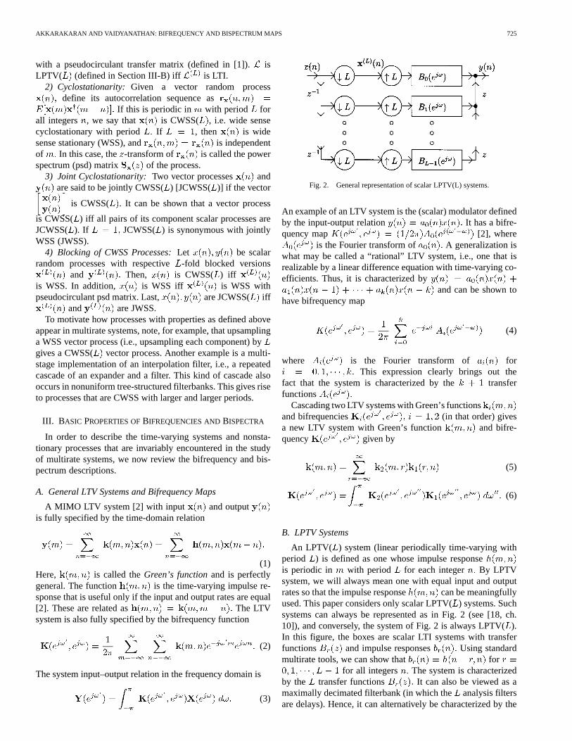
B. LPTV Systems

An LPTV( ) system (linear periodically time-varying withperiod ) is defined as one whose impulse responseis periodic in with period for each integer By LPTVsystem, we will always mean one with equal input and outputrates so that the impulse response can be meaningfullyused. This paper considers only scalar LPTV() systems. Suchsystems can always be represented as in Fig. 2 (see [18, ch.10]), and conversely, the system of Fig. 2 is always LPTV().In this figure, the boxes are scalar LTI systems with transferfunctions and impulse responses Using standardmultirate tools, we can show that for

for all integers The system is characterizedby the transfer functions It can also be viewed as amaximally decimated filterbank (in which theanalysis filtersare delays). Hence, it can alternatively be characterized by the


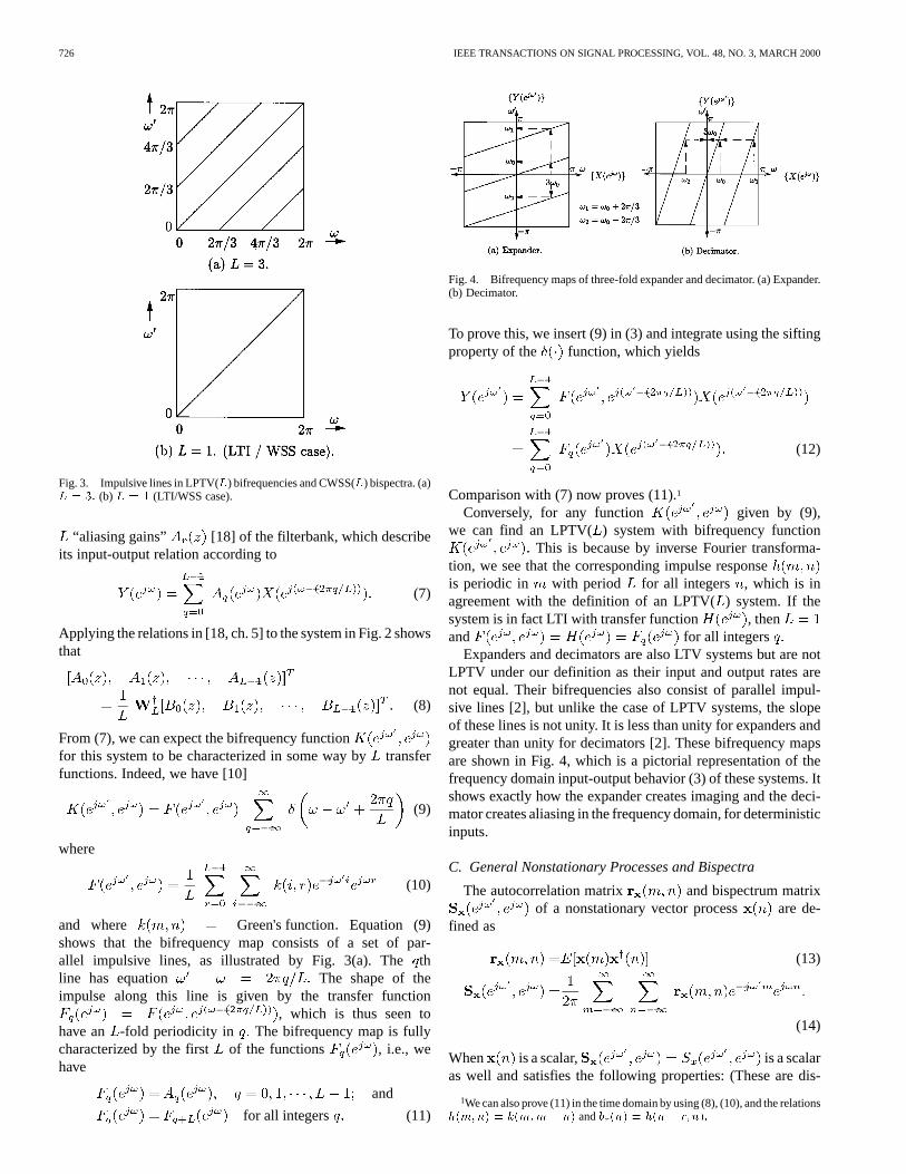
Fig. 3. Impulsive lines in LPTV(L) bifrequencies and CWSS(L) bispectra. (a)L = 3: (b) L = 1 (LTI/WSS case).

“aliasing gains” [18] of the filterbank, which describeits input-output relation according to

(7)

Applying the relations in [18, ch. 5] to the system in Fig. 2 showsthat

(8)

From (7), we can expect the bifrequency functionfor this system to be characterized in some way bytransferfunctions. Indeed, we have [10]

(9)

where

(10)

and where Green's function Equation (9)shows that the bifrequency map consists of a set of par-allel impulsive lines, as illustrated by Fig. 3(a). Thethline has equation The shape of theimpulse along this line is given by the transfer function

, which is thus seen tohave an -fold periodicity in The bifrequency map is fullycharacterized by the first of the functions , i.e., wehave

and

for all integers (11)

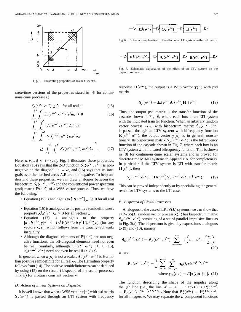
Fig. 4. Bifrequency maps of three-fold expander and decimator. (a) Expander.(b) Decimator.

To prove this, we insert (9) in (3) and integrate using the siftingproperty of the function, which yields

(12)

Comparison with (7) now proves (11).1

Conversely, for any function given by (9),we can find an LPTV( ) system with bifrequency function

This is because by inverse Fourier transforma-tion, we see that the corresponding impulse responseis periodic in with period for all integers , which is inagreement with the definition of an LPTV() system. If thesystem is in fact LTI with transfer function , thenand for all integers

Expanders and decimators are also LTV systems but are notLPTV under our definition as their input and output rates arenot equal. Their bifrequencies also consist of parallel impul-sive lines [2], but unlike the case of LPTV systems, the slopeof these lines is not unity. It is less than unity for expanders andgreater than unity for decimators [2]. These bifrequency mapsare shown in Fig. 4, which is a pictorial representation of thefrequency domain input-output behavior (3) of these systems. Itshows exactly how the expander creates imaging and the deci-mator creates aliasing in the frequency domain, for deterministicinputs.

C. General Nonstationary Processes and Bispectra

The autocorrelation matrix and bispectrum matrixof a nonstationary vector process are de-

fined as

(13)

(14)

When is a scalar, is a scalaras well and satisfies the following properties: (These are dis-

1We can also prove (11) in the time domain by using (8), (10), and the relationsh(m;n) = k(m;m� n) andb (n) = h(n � r; n):


Fig. 5. Illustrating properties of scalar bispectra.

crete-time versions of the properties stated in [4] for contin-uous-time processes.)

for all real (15)

(16)

(17)

Here, Fig. 5 illustrates these properties.Equation (15) says that the 2-D function is non-negative on the diagonal , and (16) says that its inte-grals over the hatched areas A,B are non-negative. To help un-derstand these properties, we can draw analogies between thebispectrum and the conventional power spectrum(psd) matrix of a WSS vector process. Thus, we havethe following.

• Equation (15) is analogous to for all real.

• Equation (16) is analogous to the positive semidefinitenessproperty for all vectors

• Equation (17) is analogous to the property(for any

vectors , which follows from the Cauchy–Schwartzinequality.

• Although the diagonal elements of are non-neg-ative functions, the off-diagonal elements need not evenbe real. Similarly, although (15),

need not even be real if

In general, when is not a scalar, is Hermi-tian positive semidefinite for all real. The Hermitian propertyfollows from (14). The positive semidefiniteness can be deducedby using (15) on the (scalar) bispectra of the scalar processes

for arbitrary constant vectors

D. Action of Linear Systems on Bispectra

It is well known that when a WSS vector with psd matrixis passed through an LTI system with frequency

Fig. 6. Schematic explanation of the effect of an LTI system on the psd matrix.

Fig. 7. Schematic explanation of the effect of an LTV system on thebispectrum matrix.

response , the output is a WSS vector with psdmatrix

(18)

Thus, the output psd matrix is the transfer function of thecascade shown in Fig. 6, where each box is an LTI systemwith the indicated transfer function. When an arbitrary randomvector process with bispectrum matrixis passed through an LTV system with bifrequency function

, the output vector is, in general, nonsta-tionary. Its bispectrum matrix is the bifrequencyfunction of the cascade shown in Fig. 7, where each box is anLTV system with indicated bifrequency function. This is shownin [8] for continuous-time scalar systems and is proved fordiscrete-time MIMO systems in Appendix A, for completeness.In particular if the LTV system is LTI with transfer matrix

, then

(19)

This can be proved independently or by specializing the generalresult for LTV systems to the LTI case.

E. Bispectra of CWSS Processes

Analogous to the case of LPTV() systems, we can show thata CWSS( ) random vector process has bispectrum matrix

consisting of a set of parallel impulsive lines asin Fig. 3(a). The bispectrum is given by expressions analogousto (9) and (10), namely

(20)where

where (21)

The function describing the shape of the impulse alongthe th line (i.e., the line ) is

Note thatfor all integers We may separate the component functions


that characterize the bispectrumand rewrite (20) as

(22)

From the discussion following (17), is Hermitian pos-itive-semidefinite for all real . In the special case when isWSS, , and equals the conventional psd matrixof Thus, for a WSS process with psd matrix ,the bispectrum matrix has a plot as shown in Fig. 3(b) and isgiven by

(23)

IV. A NALYSIS OF BASIC MULTIRATE BUILDING BLOCKS

This section examines the effect of basic blocks such asdecimators and expanders on the bispectrum of their stochasticinput. Some of the results will be used in the later sections toanalyze more complicated systems. Note that decimating/up-sampling of a vector means performing that operation on eachof its components.

A. Expanders, Decimators, and the Blocking Mechanism

1) Expanders:Let be a vector process obtained by-fold upsampling of the process , i.e.,

whenever is an integerotherwise.

Then, we conclude that has autocorrelation sequencethat is obtained by upsampling the autocorrela-

tion sequence of by the diagonal matrix

Thus, if and are, respectively, thebispectrum matrices of and , we have

whenever are both integersotherwise

(24)

(25)

It is well known (see Fig. 4(a) [2]) that an expander createsimaging in the frequency domain for deterministic inputs. Re-lation (25) shows that it also creates imaging in thebispectrumdomainfor arbitrary stochastic inputs(not necessarily WSS).This is shown in Fig. 8. This observation will be very useful inlater sections.

2) Decimators: Let the vector process be obtained bydecimating by , i.e., Then, the autocorre-lation sequence of is obtained by decimating that of ,i.e.,

(26)

Fig. 8. Effect of an expander on the bispectrum of a nonstationary process.

Fig. 9. Effect of a decimator on the bispectrum of a nonstationary process.

Hence, the bispectrum matrices of and are related as

(27)

Thus, the decimator creates aliasing in thebispectrum domain(Fig. 9) forstochastic inputs(possibly nonstationary), just as itcreates aliasing in the frequency domain (Fig. 4(b) [2]) for de-terministic inputs. In Fig. 9, the light shade represents the regionof support of the original bispectrum and that of its stretched-outversion (after passage through the expander). The dark–shadedareas in the output bispectrum represent overlap with shiftedcopies of the stretched version.

3) Blocking: Consider a scalar process and its -foldblocked version These are related as in Fig. 1.Thus, using (19), (25), and (27), we find that their bispectra arerelated as

(28)


and

(29)

These equations can be used to prove certain results on blockingof CWSS processes (see Section IV-B).

B. Preliminary Results

Many of the more elementary results of [1], some of whichare stated in Section II, can now be easily proved from the abovediscussion. Further, this proof technique generalizes these re-sults directly to the case of vector inputs, unlike the techniquesof [1].

• -fold upsampling of a WSS vector process gives aCWSS( ) vector process. To see this, note that thebispectrum of the WSS process has impulse lines sepa-rated by a vertical spacing of [see Fig. 3(b)]. Due tothe bispectrum domain imaging created by the expander(Fig. 8), this spacing is “compressed” to Therefore,the output has a CWSS() bispectrum as in Fig. 3(a).Note that the expander output cannot be CWSS() for

(unless the input is identically zero), i.e.,is the“fundamental period” of cyclostationarity of the output.

• -fold decimation of a CWSS() vector processgives a process that, in general, is CWSS(), where

gcd To prove this, note that the inputbispectrum is as in Fig. 3(a), with impulses along the lines

Due to the bispectrumdomain aliasing created by the decimator [which is shownin Fig. 9 and by (27)], the decimator output has impulsesalong the lines

or equivalently (30)

for (31)

where gcd These lines certainly form asubset of the set of lines

in a CWSS( ) bispectrum, and hence, the output isCWSS( ).

• A scalar process is CWSS() iff its -fold blocked ver-sion is a WSS vector. More generally, a scalar process isCWSS( ) iff its -fold blocked version is CWSS().This can be shown from (28) and (29).

V. VECTORINTERPOLATION FILTERS

This and the remaining sections analyze more complicatedinterconnections of the basic multirate building blocks of thelast section. We derive necessary and sufficient conditions fortheir outputs to be WSS for all WSS inputs. The central themein these analyses is that the multirate system fed with WSS inputcreates CWSS output by somehow adding more lines in the bis-pectrum (which is usually due to the presence of an expander).The aim is tofind the conditions under which the extra lines

Fig. 10. General vector interpolation filter.

Fig. 11. Synthesis filter bank—a special case of Fig. 10.

Fig. 12. Scalar interpolation filter—a special case of Fig. 10.

can be suppressed. The geometric insights obtained by lookingat the bispectra are exploited to find the conditions elegantly.

This section examines the-fold vector interpolation filter,which is shown in Fig. 10. This system upsamples the-com-ponent input vector by and passes the result through aMIMO LTI system with transfer matrix In gen-eral, and could be arbitrary positive integers unrelated toeach other . Fig. 11 shows the synthesis section of an

channel uniform filterbank with upsampling factor This isa special vector interpolation filter where , i.e.,is a row vector. If the vector is considered to be output inFig. 11, we get another special case where , andis square and diagonal. Finally, if in Fig. 10, we getthe usual scalar interpolation filter of Fig. 12.

For the special case of the scalar interpolation filter, [1] showsthat the output is WSS for all WSS inputs if andonly if the LTI filter has an alias-free () support. Theproof is based on the fact that a scalar process is WSS iff itsblocked versions are WSS with pseudocirculant psd matrices.This proof is quite involved and does not give any indicationabout the corresponding result for the general system of Fig. 10.This section provides a greatly simplified proof of this resultusing bispectrum analysis. We show that the new proof extendswithout much additional effort to the general case of Fig. 10.

A. MIMO Alias-free ( ) Systems

In order to state the main result on vector interpolation fil-ters, we need to define MIMO alias-free () transfer matrices.


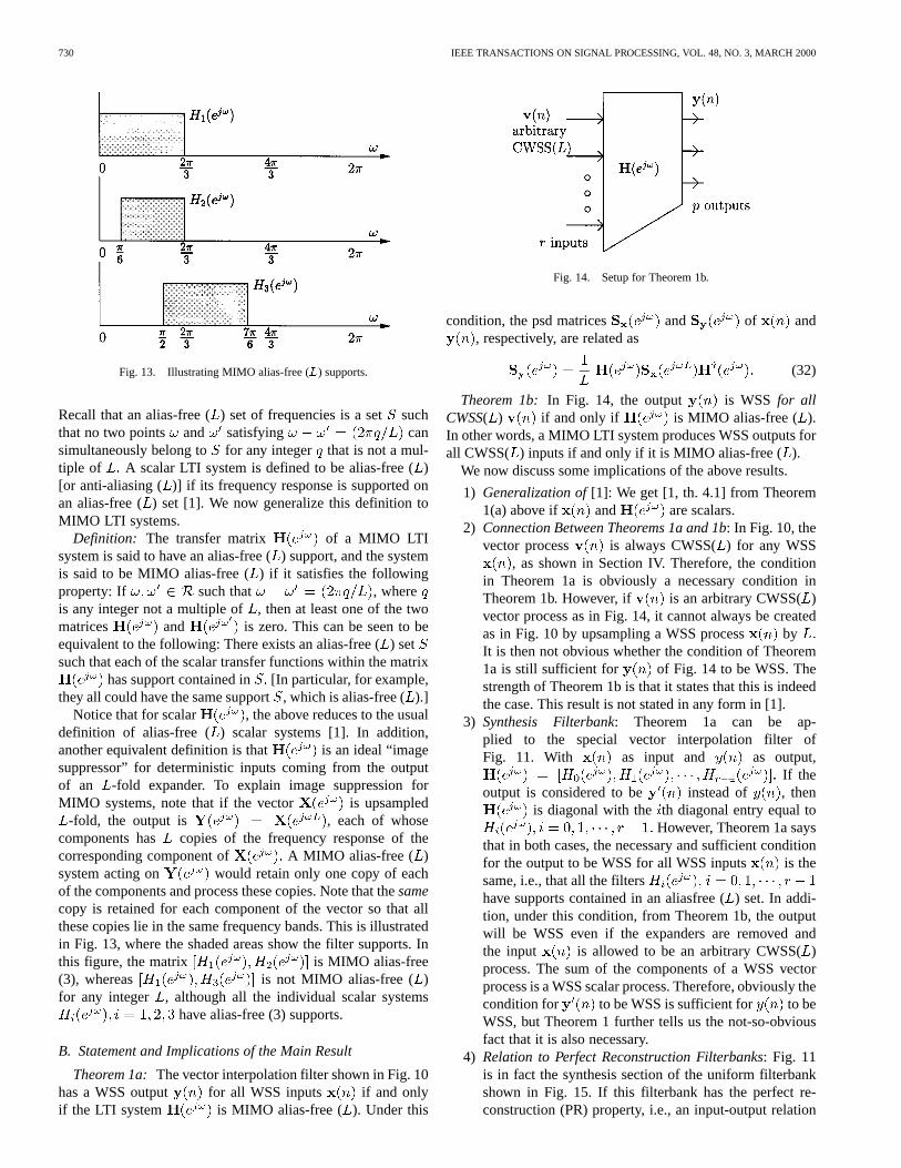
Fig. 13. Illustrating MIMO alias-free (L) supports.

Recall that an alias-free () set of frequencies is a set suchthat no two points and satisfying cansimultaneously belong to for any integer that is not a mul-tiple of A scalar LTI system is defined to be alias-free ()[or anti-aliasing ( )] if its frequency response is supported onan alias-free ( ) set [1]. We now generalize this definition toMIMO LTI systems.

Definition: The transfer matrix of a MIMO LTIsystem is said to have an alias-free () support, and the systemis said to be MIMO alias-free () if it satisfies the followingproperty: If such that , whereis any integer not a multiple of , then at least one of the twomatrices and is zero. This can be seen to beequivalent to the following: There exists an alias-free () setsuch that each of the scalar transfer functions within the matrix

has support contained in [In particular, for example,they all could have the same support, which is alias-free ().]

Notice that for scalar , the above reduces to the usualdefinition of alias-free ( ) scalar systems [1]. In addition,another equivalent definition is that is an ideal “imagesuppressor” for deterministic inputs coming from the outputof an -fold expander. To explain image suppression forMIMO systems, note that if the vector is upsampled

-fold, the output is , each of whosecomponents has copies of the frequency response of thecorresponding component of A MIMO alias-free ( )system acting on would retain only one copy of eachof the components and process these copies. Note that thesamecopy is retained for each component of the vector so that allthese copies lie in the same frequency bands. This is illustratedin Fig. 13, where the shaded areas show the filter supports. Inthis figure, the matrix is MIMO alias-free(3), whereas is not MIMO alias-free ( )for any integer , although all the individual scalar systems

have alias-free (3) supports.

B. Statement and Implications of the Main Result

Theorem 1a:The vector interpolation filter shown in Fig. 10has a WSS output for all WSS inputs if and onlyif the LTI system is MIMO alias-free ( ). Under this

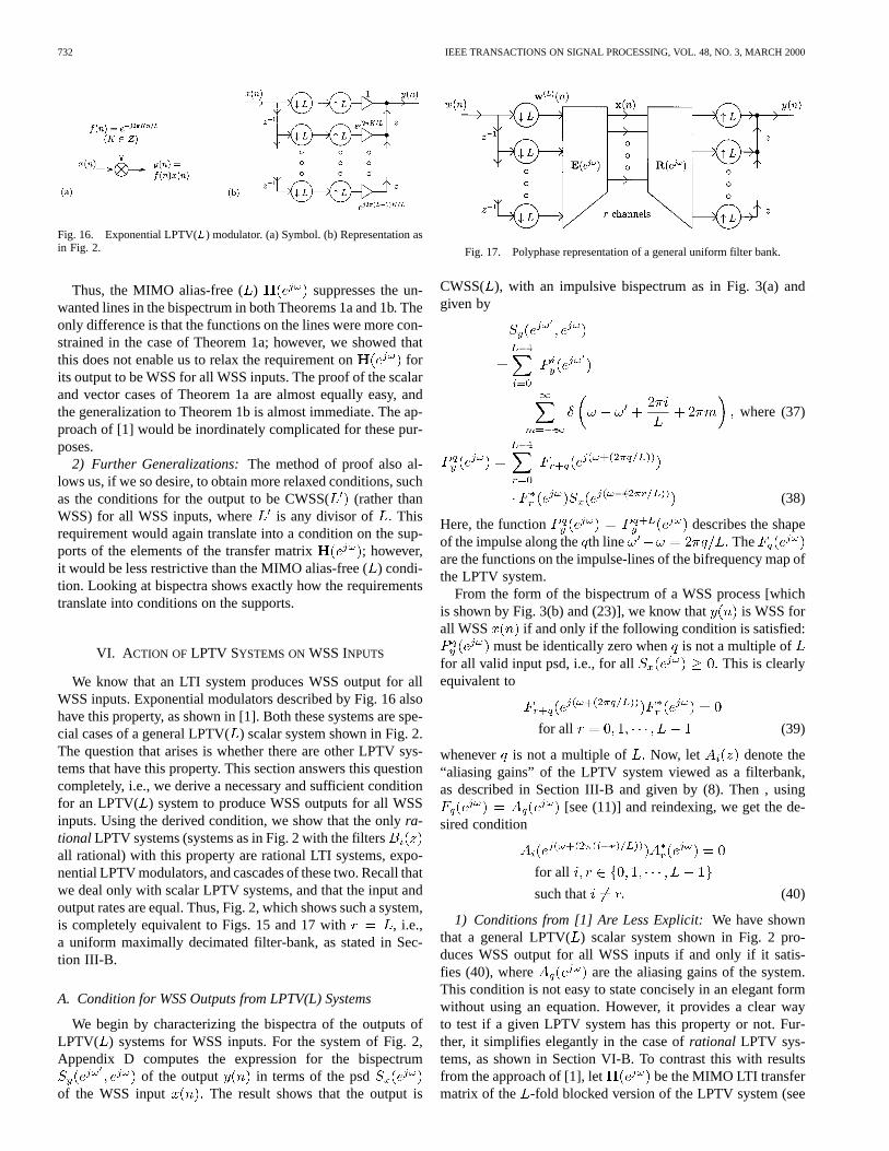
Fig. 14. Setup for Theorem 1b.

condition, the psd matrices and of and, respectively, are related as

(32)

Theorem 1b: In Fig. 14, the output is WSS for allCWSS( ) if and only if is MIMO alias-free ( ).In other words, a MIMO LTI system produces WSS outputs forall CWSS( ) inputs if and only if it is MIMO alias-free ( ).

We now discuss some implications of the above results.

1) Generalization of[1]: We get [1, th. 4.1] from Theorem1(a) above if and are scalars.

2) Connection Between Theorems 1a and 1b: In Fig. 10, thevector process is always CWSS() for any WSS

, as shown in Section IV. Therefore, the conditionin Theorem 1a is obviously a necessary condition inTheorem 1b. However, if is an arbitrary CWSS()vector process as in Fig. 14, it cannot always be createdas in Fig. 10 by upsampling a WSS process byIt is then not obvious whether the condition of Theorem1a is still sufficient for of Fig. 14 to be WSS. Thestrength of Theorem 1b is that it states that this is indeedthe case. This result is not stated in any form in [1].

3) Synthesis Filterbank: Theorem 1a can be ap-plied to the special vector interpolation filter ofFig. 11. With as input and as output,

If theoutput is considered to be instead of , then

is diagonal with theth diagonal entry equal toHowever, Theorem 1a says

that in both cases, the necessary and sufficient conditionfor the output to be WSS for all WSS inputs is thesame, i.e., that all the filtershave supports contained in an aliasfree () set. In addi-tion, under this condition, from Theorem 1b, the outputwill be WSS even if the expanders are removed andthe input is allowed to be an arbitrary CWSS()process. The sum of the components of a WSS vectorprocess is a WSS scalar process. Therefore, obviously thecondition for to be WSS is sufficient for to beWSS, but Theorem 1 further tells us the not-so-obviousfact that it is also necessary.

4) Relation to Perfect Reconstruction Filterbanks: Fig. 11is in fact the synthesis section of the uniform filterbankshown in Fig. 15. If this filterbank has the perfect re-construction (PR) property, i.e., an input-output relation


Fig. 15. General uniform filter bank.

, then clearly, the output is WSSfor all WSS inputs However, in this case, the syn-thesis filters cannot satisfy the MIMO alias-freecondition of Theorem 1 because that would imply thatall output sequences have Fourier transformwith an alias-free ( ) support (violating the PR prop-erty). This apparent conflict with Theorem 1 is resolvedby noting that it is only thefilterbank input that isallowed to be arbitrary. The input vector to thesyn-thesis sectionof the filterbank in Fig. 15 isnot an arbi-trary WSS vector process as required by Theorem 1; it isconstrained by the analysis section of the PR filterbank.The nature of this constraint is analyzed in detail in Ap-pendix B. A question arising from this is the following:What are the conditions under which is WSS for allWSS in Fig. 15? This is answered in Section VI. Inaddition, note that for PR, it is necessary that Thecase where cannot give PR and is considered inSection VII.

5) Joint Stationarity Properties: Theorem 1 allows us to an-swer questions on joint stationarity. For example, we canobtain the condition on a pair of-fold scalar interpola-tion filters for their outputs to be jointly stationary for allpairs of jointly stationary inputs. This situation is equiv-alent to that of Fig. 11 with From [1], a necessarycondition is that each filter have a support contained inan alias-free ( ) set. Theorem 1 goes further to give thefollowing necessary and sufficient condition:Both filtersupports must be contained in somecommonalias-free( ) set. Similarly, from Theorem 1a, we can further findthe necessary and sufficient condition on a pair ofvectorinterpolation filters for their outputs to be jointly WSS forall jointly WSS input pairs: All the component scalars inboththe filter transfer matrices should have supports con-tained in some common alias-free () set.

C. Proof of Theorem 1

We first prove Theorem 1a. We use (19) and (25) to computethe output bispectrum matrix in Fig. 10, as

(33)

where is the usual psd matrix of Here, we haveused (23) for the input bispectrum, and the scaling property of

the function. Now, (20) shows that is CWSS( ) andwill be WSS if and only if

whenever

for all (34)

where is the set of integers that are not multiples of[Thesystem must suppress the unwanted impulse-lines in theCWSS bispectrum to get a WSS bispectrum].

1) The Sathe–Vaidyanathan Special Case:Consider thespecial case of Fig. 12, where , and

are scalars. This is the case addressed in[1]. Here, (34) becomes

whenever

for all (35)

The output will be WSS for all WSS inputs iff(35) holds for every non-negative [This condition isnecessary because as is well known, for any transfer function

, we can find a WSS scalar random process withpsd ] Clearly, this is the same as saying that whenever

for any integer not a multiple of , thenof and , at least one is zero. This is preciselythe statement that the LTI system has an alias-free ()support. This proves the scalar result (see [1, th. 4.1]).

For the more general vector case of Fig. 10, is WSSfor all WSS iff (34) holds for every Hermitian positivesemidefinite matrix (Again, for any Hermitian pos-itive semidefinite , we can find a matrix such that

Therefore, by (18), if is a process with white un-correlated scalar components, we can form the process

with psd matrix From the definition ofMIMO alias-free ( ) systems, it is clear that if is MIMOalias-free ( ), then (34) indeed holds for every Thelemma in Appendix C shows that if (34) holds for every Hermi-tian positive definite , then of and , atleast one is the zero matrix, i.e., is MIMO alias-free ( ).This gives the converse. Finally, under the MIMO alias-free ()condition, since the output is WSS, its bispectrum (33)takes the form of (23). Comparing these equations shows thatthe psd of is indeed given by (32), as claimed. Notice thatthe lemma of Appendix C is not needed for the scalar case be-cause it is trivial there.

We now prove Theorem 1b. For this, it suffices to show thatthe MIMO alias-free ( ) property of implies thatis WSS for all CWSS( ) in Fig. 14. If is CWSS( ),the form of its bispectrum is given by (20). There-fore, using (19), the output bispectrum has the form

(36)

Comparison with (20) shows that is CWSS( ). TheMIMO alias-free ( ) condition implies that

is zero unless is a multiple of Hence, (36) takes the form of(23), i.e., is WSS.


Fig. 16. Exponential LPTV(L) modulator. (a) Symbol. (b) Representation asin Fig. 2.

Thus, the MIMO alias-free () suppresses the un-wanted lines in the bispectrum in both Theorems 1a and 1b. Theonly difference is that the functions on the lines were more con-strained in the case of Theorem 1a; however, we showed thatthis does not enable us to relax the requirement on forits output to be WSS for all WSS inputs. The proof of the scalarand vector cases of Theorem 1a are almost equally easy, andthe generalization to Theorem 1b is almost immediate. The ap-proach of [1] would be inordinately complicated for these pur-poses.

2) Further Generalizations:The method of proof also al-lows us, if we so desire, to obtain more relaxed conditions, suchas the conditions for the output to be CWSS((rather thanWSS) for all WSS inputs, where is any divisor of Thisrequirement would again translate into a condition on the sup-ports of the elements of the transfer matrix ; however,it would be less restrictive than the MIMO alias-free () condi-tion. Looking at bispectra shows exactly how the requirementstranslate into conditions on the supports.

VI. A CTION OF LPTV SYSTEMS ONWSS INPUTS

We know that an LTI system produces WSS output for allWSS inputs. Exponential modulators described by Fig. 16 alsohave this property, as shown in [1]. Both these systems are spe-cial cases of a general LPTV() scalar system shown in Fig. 2.The question that arises is whether there are other LPTV sys-tems that have this property. This section answers this questioncompletely, i.e., we derive a necessary and sufficient conditionfor an LPTV( ) system to produce WSS outputs for all WSSinputs. Using the derived condition, we show that the onlyra-tional LPTV systems (systems as in Fig. 2 with the filtersall rational) with this property are rational LTI systems, expo-nential LPTV modulators, and cascades of these two. Recall thatwe deal only with scalar LPTV systems, and that the input andoutput rates are equal. Thus, Fig. 2, which shows such a system,is completely equivalent to Figs. 15 and 17 with , i.e.,a uniform maximally decimated filter-bank, as stated in Sec-tion III-B.

A. Condition for WSS Outputs from LPTV(L) Systems

We begin by characterizing the bispectra of the outputs ofLPTV( ) systems for WSS inputs. For the system of Fig. 2,Appendix D computes the expression for the bispectrum

of the output in terms of the psdof the WSS input The result shows that the output is

Fig. 17. Polyphase representation of a general uniform filter bank.

CWSS( ), with an impulsive bispectrum as in Fig. 3(a) andgiven by

where (37)

(38)

Here, the function describes the shapeof the impulse along theth line Theare the functions on the impulse-lines of the bifrequency map ofthe LPTV system.

From the form of the bispectrum of a WSS process [whichis shown by Fig. 3(b) and (23)], we know that is WSS forall WSS if and only if the following condition is satisfied:

must be identically zero whenis not a multiple offor all valid input psd, i.e., for all This is clearlyequivalent to

for all (39)

whenever is not a multiple of Now, let denote the“aliasing gains” of the LPTV system viewed as a filterbank,as described in Section III-B and given by (8). Then , using

[see (11)] and reindexing, we get the de-sired condition

for all

such that (40)

1) Conditions from [1] Are Less Explicit:We have shownthat a general LPTV() scalar system shown in Fig. 2 pro-duces WSS output for all WSS inputs if and only if it satis-fies (40), where are the aliasing gains of the system.This condition is not easy to state concisely in an elegant formwithout using an equation. However, it provides a clear wayto test if a given LPTV system has this property or not. Fur-ther, it simplifies elegantly in the case ofrational LPTV sys-tems, as shown in Section VI-B. To contrast this with resultsfrom the approach of [1], let be the MIMO LTI transfermatrix of the -fold blocked version of the LPTV system (see


Section II). In addition, let be the psd matrix of theblocked version of [which is pseudocirculant as

is WSS]. The approach of [1] would use (18) to state thecondition as follows: must be pseudo-circulant for every pseudocirculant positive semidefinite matrix

[i.e., for every possible valid psd matrix ofunder the constraint that is WSS]. This statement

gives a veryimplicit condition on the LPTV system and cannotbe easily tested.

2) LTI Case: The LPTV( ) system of Fig. 2 becomes LTIwith transfer function if and only if all the filtersequal From (8), this is equivalent to

, which means that (40) is satisfied. Therefore,such a system indeed produces WSS output for all WSS inputs,which is a well known fact.

3) Exponential Modulator:A general scalar modulator is asystem with output for input An expo-nential modulator is one with This is LPTV( )if and only if for some integer Such a systemis shown in Fig. 16(a). We know [1] that any exponential modu-lator produces a WSS output for all WSS inputs Toreconcile this result with (40), note that an LPTV() exponen-tial modulator can be represented as in Fig. 16(b). This is likethe general structure of Fig. 2 with a constant multiplierof value Therefore, (8) shows that is nonzero(and constant) for exactly one value ofThis means that (40) is indeed satisfied here.

B. Case of Rational LPTV Systems

Rational LPTV( ) systems are systems as in Fig. 2 with allthe filters being rational LTI filters. Special cases are ra-tional LTI systems [where all ] and expo-nential LPTV( ) modulators Cascadesof rational LPTV(L) systems are also rational LPTV(L)—thisis evident when we consider the-fold blocked versions of thesystems (which are LTI as seen in Section II).

It is well known that the special cases of rational LTI systemsand exponential LPTV() modulators produce WSS outputs forall WSS inputs, and hence, so do cascades of these systems. Thequestion arises whether there are other rational LPTV() sys-tems with this property. This can be answered using the generalcondition (40) derived above. We have the following theorem.

Theorem 2: A rational LPTV( ) scalar system producesWSS outputs for all WSS inputs if and only if it is either arational LTI system, an exponential LPTV() modulator, or acascade of these.

Proof: From the earlier discussion, we see that it sufficesto prove the “only if” part of the theorem. We need the relationbetween the aliasing gains and the filters ofthe LPTV( ) system. This relation is given by (8) and is repro-duced here for convenience:

(41)

This equation shows that rationality of the is equivalentto that of the Now, consider a rational LPTV() system

Fig. 18. Illustrating the proof of Theorem 2. (a) Rational LPTV(L) systemproducing WSS output for all WSS inputs. (b) Equivalent structure for thissystem.

producing WSS output for all WSS inputs. Thus, are ra-tional and satisfy the condition (40). This is possible if and onlyif there is at most one such thatis not identically zero. Excluding the trivial case when there isno such , let be not identically zero. [ isrational]. Using (41), this means that each in Fig. 2 is thecascade of a constant multiplier and Thus, thesystem has the structure shown in Fig. 18(a), which shows itselfto be equivalent to Fig. 18(b) on comparison with Fig. 16. Thus,the system is indeed a cascade of an exponential LPTV() mod-ulator followed by the rational LTI system This concludesthe proof.

VII. OTHER APPLICATIONS

A. Partial Reconstructions from Subbands of a FB

Principal component filterbanks were proposed in [19],with the idea of compressing the main signal features into afew subbands of the filterbank and dropping the remainingsubbands. This results in a partial reconstruction of the signal,and the system producing this reconstruction is equivalent to anoverdecimated uniform filterbank, i.e., a system as in Fig. 15,where Theorem 2 then says that given any rationaluniform maximally decimated filterbank, none of the partial(or principal component) reconstructions can be WSS for allWSS inputs. For if this were the case, the system creatingthe reconstruction (an overdecimated rational filterbank)would have to be a cascade of a modulator and an LTI system(from Theorem 2). However, such a cascade is necessarily amaximally decimatedfilterbank, which is a contradiction.

B. Nonrational LPTV Systems

If we relax the restriction of rationality, we can find moreexamples of LPTV( ) systems producing WSS output for allWSS inputs. The ideal uniform brickwall subband coder is anexample of a nonrational filterbank for which the systems pro-ducing the partial reconstructions are also LTI. Thus, in thiscase, every partial reconstruction is WSS if the input is WSS.Systems as in Fig. 2 where the vector of filters isMIMO alias-free ( ) are another class of systems that produceWSS output for all WSS inputs, as is clear from using The-orem 1a. Indeed, (41) shows that for such systems the vectorof aliasing gains is also MIMO alias-free ( ); hence,the condition (40) is satisfied. In fact Theorem 1a shows that


this class of systems is also the class for which the outputis WSS forarbitrary CWSS( ) scalar inputs

C. Characterization of CWSS Scalar Bispectra

The equations (37) and (38) give a full characterization ofthe bispectrum of an arbitrary CWSS(L) scalar processThis is because by spectral factorization of the psd matrix ofthe blocked version of , we can show that every CWSS()scalar process can be obtained by passing (WSS) white noisethrough an appropriate LPTV() system. In particular, thismeans that from (37) and (38) will automaticallysatisfy the properties (15)–(17) for arbitrary transfer func-tions for any non-negative function (i.e., valid psd)

D. Bifrequency Characterization of Lossless LTV Systems

Lossless LTI systems have been extensively studied in theliterature, owing to connections with paraunitary filterbanksand orthonormal wavelets. Losslessness of a causal stable LTIsystem may be described by two equivalent definitions.

1) The system input and output “energies” norms) arealways equal.

2) The inverse of the system is , which is the so-calledparaconjugate, defined so that

The extension to LTV systems is described in [5] and [6] in con-nection with time-varying paraunitary filterbanks. Using the no-tation of [5], the above definitions apply and are shown to beequivalent for LTV systems as well, except that we have a newdefinition of the “paraconjugate” of the LTV system

Converting this definition from [5] into the notationusing the Green’s function , we find that the paraconju-gate is the system with Green’s functionThis system is called the adjoint or dual system in [2]. Thus,using (5) and (6), the second definition above for a lossless LTVsystem now reads as

(42)

(43)

(Here, is the discrete impulse sequence.) This notationis more general since the notation of [5] is useful only if theinput and output rates of the LTV system are equal. For example,the -fold expander is a lossless LTV system that necessarilyrequires this notation. For this system,[2], which is easily seen to satisfy (42). This is consistent withthe fact that the expander is lossless.

The term “adjoint” here has the same meaning as in operatortheory: If are inner-product spaces, the adjoint of a linearoperator is the operator satisfying

for all (whereis the innerproduct of the two vectors from the same

inner-product space). Now, viewing the LTV systemas an operator from to , we can show on lines sim-ilar to [5] that the adjoint of this operator is the LTV system

Thus, general lossless LTV systems areoperatorswhose inverses are their adjoints.

VIII. C ONCLUDING REMARKS

We have used bifrequencies and bispectra to study the ef-fects of multirate systems on the statistics of random input sig-nals. We have shown that this often yields more insight intothe working of these systems than other approaches based onpolyphase matrices and pseudocirculants. It allows easy gen-eralization of many of the results of [1] to MIMO systems. Itallows us to prove two nontrivial results (Theorems 1 and 2)and seems to be a powerful tool for answering questions like“When does a multirate system produce WSS outputs for allWSS inputs?” However, as with any tool, indiscriminate useof bifrequency analysis may be inefficient in many situations.What appears to make it especially useful is the geometric in-sight obtained when LPTV systems and CWSS processes areinvolved, causing the 2-D Fourier transforms to become impul-sive lines.

One question arising from our analysis is the following: Canthese results be used to tell us more about lossless LTV sys-tems described in [5]? We have pointed out the bifrequencycharacterization of a general lossless LTV system. However,the bifrequency function is so general that it is not immediatelyclear whether this helps in any way. A special case that mightbe considered is that of lossless LPTV systems. Scalar sys-tems of this kind have been dealt with in this paper. Vector sys-tems correspond to paraunitary periodically time-varying filter-banks, where the analysis and synthesis filterbanks are switchedcyclically between a selection of banks. Bifrequency analysisof these may lead to some new insights. Another special casemight be that of “rational” LTV systems, i.e., those realizableby a linear difference equation with time-varying coefficients.The bifrequency function for such a system, which is given by(4), clearly reflects the fact that it is fully characterized by thecoefficients of the difference equation (unlike the representa-tion in [5]). Another area where bifrequency analysis might beuseful is in the theory of matrix filterbanks described in [20].We could also ask other questions further generalizing the is-sues considered here, e.g., find all LTV (as opposed to LPTV)systems producing WSS outputs for all WSS inputs. The answerto this is not directly evident from using bispectra. For example,arbitrary exponential modulators (not necessarily LPTV) alsofall in this class [1].

APPENDIX A

Here, we prove the rule expressed by Fig. 7 for determiningthe effect of a general LTV system on the bispectrum of its input.Let the processes and be, respectively, the input andoutput of an LTV system represented by its Green’s function

Equations (1) and (2) are therefore satisfied. Define


the autocorrelation sequences andUsing (1), we have

where (44)

(45)

By comparison with (5), in (45) is the Green’s functionof the cascade of the LTV systems with Green’s functions

and (in that order). Similarly, theoutput autocorrelation in (44) is the Green’s functionof the cascade of the LTV systems represented byand (in that order). Hence, the 2-D Fourier transformof , i.e., the output bispectrum, is the bifrequencyfunction of this cascade. Drawing the cascades and replacingGreen’s functions with bifrequency functions yields Fig. 7.

APPENDIX B

This appendix serves to show that if the filterbank in Fig. 15has the PR property, the vector input to its synthesis sec-tion isnotan arbitrary WSS vector process even if the filterbankinput is an arbitrary WSS scalar process. To do this, weredraw Fig. 15 as in Fig. 17, where and are the anal-ysis and synthesis polyphase matrices of the filterbank. We cannow use (18) to show that the psd matrix of is

Here, is the psd matrix ofthe blocked vector in Fig. 17, and is thus pseudocircu-lant since is WSS. Now, PR implies that is invert-ible (for all ); hence, cannot be an arbitrary positivesemidefinite matrix. For example, if is positive semidef-inite but not pseudocirculant, then is anexample of a positive semidefinite matrix that cannotequal because cannot equal

APPENDIX C

Lemma 1: If are fixed matrices of the same size suchthat for every Hermitian positive definite matrix ,then either or (or both).

To prove the lemma, first consider the case whenand are column vectors. Assuming both are nonzero, wewill establish a contradiction. Choosing shows that thevectors are orthogonal, i.e., However, we caneasily find a linear transform that acts on these vectors to pro-duce two nonorthogonal nonzero vectors. To be specific, letbe any two independent nonzero nonorthogonal column vectorsof same size as Then, we can find a nonsingular squarematrix such that and Since ,taking (which is Hermitian positive definite) yields

, which is a contradiction. [To find the matrix

here, suppose , which is the space of all -tuples.Extend the linearly independent set to a basis of ,and use the basis elements as columns of a matrixThus,is nonsingular with first two columns Repeat the sameconstruction starting with to get a nonsingularmatrix with first two columns Then, is asatisfactory choice.]

Next, we use the above to prove by contradiction thegeneral case, i.e., , and

, where are columnvectors of the same size. If both are nonzero, we can find

such that both and are nonzero.Now, for all Hermitian positive definite , ,and therefore, its entry is zero as well. This isimpossible by the established statement of the lemma when

are column vectors. This completes the proof.

APPENDIX D

This appendix serves to prove (37) and (38). As explainedin Section III-D, is the bifrequency function ofthe cascade of Fig. 7, where is ascalar given by (9), and

(46)

which is (23) in scalar form. By (6), the cascade ofand has bifrequency func-

tion

(47)

(48)

Using the sifting property of the function and the definition, we get

(49)

(50)

One more application of (6) to cascade withyields

(51)

(52)


Using (46) and (50), we get

(53)

(54)

We now use the -fold periodicity of the summand in the indexto replace with throughout the summand. The inner

sum over then becomes independent ofUsing, this yields

(55)

This is identical to (37) with defined as in (38). Thiscompletes the derivation of (37) and (38).

REFERENCES

[1] V. P. Sathe and P. P. Vaidyanathan, “Effects of multirate systems on thestatistical properties of random signals,”IEEE Trans. Signal Processing,vol. 41, pp. 131–146, Jan. 1993.

[2] R. E. Crochiere and L. R. Rabiner,Multirate Digital Signal Pro-cessing. Englewood Cliffs, NJ: Prentice-Hall, 1983.

[3] L. A. Zadeh, “Frequency analysis of variable networks,”Proc. IRE, vol.32, pp. 291–299, Mar. 1950.

[4] A. Papoulis, Probability, Random Variables, and Stochastic Pro-cesses. New York: McGraw-Hill, 1965.

[5] S.-M. Phoong and P. P. Vaidyanathan, “Time-varying filters and filterbanks: Some basic principles,”IEEE Trans. Signal Processing, vol. 44,pp. 2971–2987, Dec. 1996.

[6] , “Factorability of lossless time-varying filters and filter banks,”IEEE Trans. Signal Processing, vol. 45, pp. 1971–1986, Aug. 1997.

[7] J. Tuqan and P. P. Vaidyanathan, “Oversampling PCM techniques andoptimum noise shapers for quantizing a class of nonbandlimited sig-nals,” IEEE Trans. Signal Processing, vol. 47, pp. 389–407, Feb. 1999.

[8] A. Blanc-Lapierre and R. Fortet,Theory of Random Functions, J. Gani,Ed. Newark, NJ: Breach, 1968, vol. I and II.

[9] C. L. Nikias and J. M. Mendel, “Introduction to ‘Special section onhigher order spectral analysis,,”IEEE Trans. Acoust., Speech, SignalProcessing, vol. 38, pp. 1236–1237, July 1990.

[10] C. M. Loeffler and C. S. Burrus, “Optimal design of periodicalytime-varying and multirate digital filters,”IEEE Trans. Acoust., Speech,Signal Processing, vol. ASSP-32, pp. 991–997, Oct. 1984.

[11] W. A. Gardner,Introduction to Random Processes with Applications toSignals and Systems. New York: McGraw-Hill, 1989.

[12] , “Exploitation of spectral redundancy in cyclostationary signals,”IEEE Signal Processing Mag., Apr. 1991.

[13] S. Ohno and H. Sakai, “Optimization of filter banks using cyclosta-tionary spectral analysis,”IEEE Trans. Signal Processing, vol. 44, pp.2718–2725, Nov. 1996.

[14] H. Sakai and S. Ohno, “Theory of cyclostationary processes andits applications,” inStatistical Methods in Control and Signal Pro-cessing. New York: Marcel Dekker, 1997, ch. 12.

[15] U. Petersohn, N. J. Fliege, and H. Unger, “Exact analysis of aliasingeffects and nonstationary quantization noise in multirate systems,” inProc. IEEE ICASSP, vol. III, Adelaide, Australia, 1994, pp. 173–176.

[16] U. Petersohn, H. Unger, and N. J. Fliege, “Exact deterministic and sto-chastic analysis of multirate systems with application to fractional sam-pling rate alteration,” inProc. IEEE ISCAS, vol. II, London, U.K., 1994,pp. 177–180.

[17] L. Izzo and A. Napolitano, “Multirate processing of time series ex-hibiting higher order cyclostationarity,”IEEE Trans. Signal Processing,vol. 46, pp. 429–439, Feb. 1998.

[18] P. P. Vaidyanathan,Multirate Systems and Filter Banks. EnglewoodCliffs, NJ: Prentice-Hall, 1993.

[19] M. K. Tsatsanis and G. B. Giannakis, “Principal component filter banksfor optimal multiresolution analysis,”IEEE Trans. Signal Processing,vol. 43, pp. 1766–1777, Aug. 1995.

[20] V. M. Gadre and R. K. Patney, “Vector multirate filtering and matrixfilter banks,” inProc. IEEE Int. Symp. Circuits Syst.San Diego, CA,May 1992, pp. 1360–1363.

Sony Akkarakaran was born in Thrissur, India, in1975. He received the B.Tech degree from the In-dian Institute of Technology, Bombay, in 1996 andthe M.S. degree from the California Institute of Tech-nology, Pasadena, in 1997, both in electrical engi-neering. He is currently pursuing the Ph.D. degree inthe field of digital signal processing at the CaliforniaInstitute of Technology.

His research interests are multirate systems,wavelets, and their communications applications.

P. P. Vaidyanathan(S’80–M’83–SM’88–F’91) wasborn in Calcutta, India, on October 16, 1954. Hereceived the B.Sc. (Hons.) degree in physics and theB.Tech. and M.Tech. degrees in radiophysics andelectronics, all from the University of Calcutta, in1974, 1977, and 1979, respectively, and the Ph.D.degree in electrical and computer engineering fromthe University of California, Santa Barbara, in 1982.

He was a Postdoctoral Fellow at the University ofCalifornia, Santa Barbara, from Sepember 1982 toMarch 1983. In March 1983, he joined the Depart-

ment of Electrical Engineering, California Institute of Technology, Pasadena,as an Assistant Professor, and since 1993, he has been Professor of ElectricalEngineering there. His main research interests are in digital signal processing,multirate systems, wavelet transforms, and adaptive filtering.

Dr. Vaidyanathan served as Vice-Chairman of the Technical Program Com-mittee for the 1983 IEEE International Symposium on Circuits and Systemsand as the Technical Program Chairman for the 1992 IEEE International Sym-posium on Circuits and Systems. He was an Associate Editor for the IEEETRANSACTIONS ONCIRCUITS AND SYSTEMSfrom 1985 to 1987 and is currentlyon Associate Editor for the IEEE SIGNAL PROCESSINGLETTERS and a Con-sulting Editor forApplied and Computational Harmonic Analysis. He was aGuest Editor in 1998 for Special Issues of the IEEE TRANSACTIONS ONSIGNAL

PROCESSINGand the IEEE TRANSACTIONS ONCIRCUITS AND SYSTEMSII on thetopics of filter banks, wavelets, and subband coders. He has authored a numberof papers in IEEE journals and is the author of the bookMultirate Systems andFilter Banks(Englewood Cliffs, NJ: Prentice-Hall, 1993). He has written sev-eral chapters for various signal processing handbooks. He was a recipient of theAward for Excellence in Teaching from the California Institute of Technologyfor the years 1983 to 1984, 1992 to 1993, and 1993 to 1994. He also receivedthe NSF’s Presidential Young Investigator award in 1986. In 1989, he receivedthe IEEE ASSP Senior Award for his paper on multirate perfect-reconstruc-tion filter banks. In 1990, he was recipient of the S. K. Mitra Memorial Awardfrom the Institute of Electronics and Telecommunications Engineers of Indiafor his joint paper in the IETE journal. He was also the coauthor of a paper onlinear-phase perfect reconstruction filter banks in the IEEE TRANSACTIONS ON

SIGNAL PROCESSING, for which the first author (T. Nguyen) received the YoungOutstanding Author award in 1993. He received the 1995 F. E. Terman Award ofthe American Society for Engineering Education, sponsored by Hewlett PackardCo., for his contributions to engineering education. He has given several plenarytalks at such conferences as the EUSIPCO’98, ASIMOLAR’88, and SPCOM’95conferences on signal processing. He was a Distinguished Lecturer of the IEEESignal Processing Society from 1996 to 1997.

Bifrequency and bispectrum maps: a new look at multirate ... · Bifrequency and Bispectrum Maps: A...

Documents

Transcript of Bifrequency and bispectrum maps: a new look at multirate ... · Bifrequency and Bispectrum Maps: A...