BGP Evolution Analysis

Tim BlankersVrije Universiteit

AmsterdamThe Netherlands

t.blankers@student.vu.nl

Supervisors:Benno Overeinder, NLnet Labs, Amsterdam

Spyros Voulgaris, Vrije Universiteit, Amsterdam

June 24, 2014

Abstract

The Internet has been growing rapidly for many years. The routing protocol is keeping trackof changes throughout the network every day to assure connectivity between communicatingend points. A logical consequence of the growth trend is the increase in effort to discoverreachability of all the networks. Networks send update messages to each other to inform aboutnew or changed paths to other networks. The routing table at each router in the network keepstrack of the routes to designated networks. As it turns out the size of the global routing tablegrows at a faster rate than the amount of update messages being send per day. This paperinvestigates the different components which together form the actual update message signaland tries to find a reason behind the faster growth.

1

Contents

1 Introduction 41.1 BGP . . . . . . . . . . . . . . . . . . . . . . . . . . . . . . . . . . . . . . . . . . . . . 41.2 Problem Definition . . . . . . . . . . . . . . . . . . . . . . . . . . . . . . . . . . . . . 41.3 Hypotheses . . . . . . . . . . . . . . . . . . . . . . . . . . . . . . . . . . . . . . . . . 41.4 Approach . . . . . . . . . . . . . . . . . . . . . . . . . . . . . . . . . . . . . . . . . . 51.5 Importance . . . . . . . . . . . . . . . . . . . . . . . . . . . . . . . . . . . . . . . . . 5

2 Interdomain Routing 62.1 History . . . . . . . . . . . . . . . . . . . . . . . . . . . . . . . . . . . . . . . . . . . . 62.2 BGP . . . . . . . . . . . . . . . . . . . . . . . . . . . . . . . . . . . . . . . . . . . . . 62.3 Autonomous Systems . . . . . . . . . . . . . . . . . . . . . . . . . . . . . . . . . . . . 62.4 Prefixes . . . . . . . . . . . . . . . . . . . . . . . . . . . . . . . . . . . . . . . . . . . 72.5 Routing table . . . . . . . . . . . . . . . . . . . . . . . . . . . . . . . . . . . . . . . . 72.6 Policies/Communities . . . . . . . . . . . . . . . . . . . . . . . . . . . . . . . . . . . . 8

3 Related Work 9

4 Methods 114.1 Fetch and Parse . . . . . . . . . . . . . . . . . . . . . . . . . . . . . . . . . . . . . . . 11

5 Results 135.1 Growth Trends . . . . . . . . . . . . . . . . . . . . . . . . . . . . . . . . . . . . . . . 13

5.1.1 2005 to 2013 . . . . . . . . . . . . . . . . . . . . . . . . . . . . . . . . . . . . . 135.1.2 2013 . . . . . . . . . . . . . . . . . . . . . . . . . . . . . . . . . . . . . . . . . 17

5.2 Top Talkers . . . . . . . . . . . . . . . . . . . . . . . . . . . . . . . . . . . . . . . . . 175.2.1 Top Talking Peers . . . . . . . . . . . . . . . . . . . . . . . . . . . . . . . . . . 175.2.2 Top Talking Originating ASes . . . . . . . . . . . . . . . . . . . . . . . . . . . 195.2.3 Top Talking Prefixes . . . . . . . . . . . . . . . . . . . . . . . . . . . . . . . . 205.2.4 2005-2013 . . . . . . . . . . . . . . . . . . . . . . . . . . . . . . . . . . . . . . 21

5.3 Distributions of updates . . . . . . . . . . . . . . . . . . . . . . . . . . . . . . . . . . 215.4 The Core . . . . . . . . . . . . . . . . . . . . . . . . . . . . . . . . . . . . . . . . . . 24

5.4.1 Days . . . . . . . . . . . . . . . . . . . . . . . . . . . . . . . . . . . . . . . . . 255.4.2 Months . . . . . . . . . . . . . . . . . . . . . . . . . . . . . . . . . . . . . . . 265.4.3 AS9304 . . . . . . . . . . . . . . . . . . . . . . . . . . . . . . . . . . . . . . . 295.4.4 Years . . . . . . . . . . . . . . . . . . . . . . . . . . . . . . . . . . . . . . . . . 30

5.5 Detecting Level Shifts . . . . . . . . . . . . . . . . . . . . . . . . . . . . . . . . . . . 315.5.1 Burstiness . . . . . . . . . . . . . . . . . . . . . . . . . . . . . . . . . . . . . . 325.5.2 Plotting Variance . . . . . . . . . . . . . . . . . . . . . . . . . . . . . . . . . . 325.5.3 Clusters . . . . . . . . . . . . . . . . . . . . . . . . . . . . . . . . . . . . . . . 345.5.4 Nodes causing the level shift . . . . . . . . . . . . . . . . . . . . . . . . . . . . 355.5.5 Causation . . . . . . . . . . . . . . . . . . . . . . . . . . . . . . . . . . . . . . 365.5.6 Other irregularities . . . . . . . . . . . . . . . . . . . . . . . . . . . . . . . . . 37

5.6 Layers . . . . . . . . . . . . . . . . . . . . . . . . . . . . . . . . . . . . . . . . . . . . 385.6.1 Duplicates . . . . . . . . . . . . . . . . . . . . . . . . . . . . . . . . . . . . . . 385.6.2 Community Information . . . . . . . . . . . . . . . . . . . . . . . . . . . . . . 385.6.3 Community Updates . . . . . . . . . . . . . . . . . . . . . . . . . . . . . . . . 405.6.4 Events . . . . . . . . . . . . . . . . . . . . . . . . . . . . . . . . . . . . . . . . 415.6.5 Timeout . . . . . . . . . . . . . . . . . . . . . . . . . . . . . . . . . . . . . . . 425.6.6 Visualizing Events . . . . . . . . . . . . . . . . . . . . . . . . . . . . . . . . . 42

2

6 Aggregated Analysis and Conclusions 456.1 Top-down . . . . . . . . . . . . . . . . . . . . . . . . . . . . . . . . . . . . . . . . . . 456.2 Monitoring . . . . . . . . . . . . . . . . . . . . . . . . . . . . . . . . . . . . . . . . . . 45

7 Summary 47

A Appendix A 50A.1 Graph Files . . . . . . . . . . . . . . . . . . . . . . . . . . . . . . . . . . . . . . . . . 50A.2 Layer Files . . . . . . . . . . . . . . . . . . . . . . . . . . . . . . . . . . . . . . . . . . 51

B Appendix B 51B.0.1 graph.py . . . . . . . . . . . . . . . . . . . . . . . . . . . . . . . . . . . . . . . 51B.0.2 growth.py . . . . . . . . . . . . . . . . . . . . . . . . . . . . . . . . . . . . . . 51B.0.3 hist.py . . . . . . . . . . . . . . . . . . . . . . . . . . . . . . . . . . . . . . . . 51B.0.4 top.py . . . . . . . . . . . . . . . . . . . . . . . . . . . . . . . . . . . . . . . . 51

3

1 Introduction

1.1 BGP

The Border Gateway Protocol (BGP) is the primary global routing protocol used in today’s Internet.It routes traffic over different administrative domains, while each domain is controlling a collectionof routing prefixes. Each of these domains, or Autonomous Systems (ASes) is under the controlof at least one network operator, whom defines its set of policies. The way BGP routes traffic isdetermined by these policies. An AS may notify its direct neighbours (peers) of the routing prefixesit originates through the use of announcements and withdrawals.

The amount of ASes along with the prefixes and possible routes grows every day [2]. Each AS has tomaintain its own administration of all prefixes and routes in its routing table. A logical consequenceof the growth of the network is the constant increase in complexity of the routing table. Discussionsabout the scalability of BGP have been taking place for quite a while [3]. Given the vast size ofthe Internet it is hard to perform data analysis and trend prediction [4]. The stability and correctfunctioning of the Internet is of such great importance that there is a need for detecting possiblesevere issues before they actually occur.

1.2 Problem Definition

Some previous studies on the growth of BGP have shown fairly comforting results [5][6]. Althoughthe size of the routing table grows at a fast rate, the amount of BGP updates the ASes have toprocess (the “churn”) grows at a much slower rate. To get a better understanding of the dynamicsof BGP, it is crucial to investigate the churn’s composition. If there are several distinctive layersfound in the update rate over an extensive period of time, BGP becomes a lot easier to manage andanalyze. By concisely identifying the constant factors in the dynamics of BGP it is also possible todetect any out of the ordinary behaviour. This could in turn be used to pinpoint “level shifts” [6].This leads to the following three research questions:

1. Why does BGP churn grow at such a slower rate than the size of the routing table?

2. Is it possible to partition BGP churn into several distinct layers?

3. How are irregularities reliably detected?

To investigate the dynamics of BGP, data about its internal structure has to be collected. Currentlyit is practically impossible to get a perfect snapshot of the Internet. Not only would it require aimmense amount of storage, but there would have to be data collectors at each AS as well. Giventhe fact that there are currently around 46,000 ASes and 500,000 prefixes [2], it is a lot more sensibleto just focus on a perspective relative to an observation point. Consequently this means the analyseson BGP will never be flawless. Investigating the Internet will always imply the use of abstractions,heuristics and incomplete data [7]. Thus generalizing behaviour seen from a specific perspective ofthe Internet to BGP as a whole should be done with great caution.

1.3 Hypotheses

Since drawing general conclusions from specific experiments is so hard, conclusions from currentresearch projects may be taken with a grain of salt. The slower growth of BGP churn could possiblybe attributed to the effects of analyzing a specific AS. In the case of AS131072 analyzed by Geoff

4

Huston, the slow growth could be explained by its specific location, namely the edge of the network.Other ASes with different perspectives may exhibit different behaviour.

Finding constant layers in the BGP update rate may prove to be very difficult. It has been shown thatthe announcement rate is very volatile [6]. This combined with the enormous amount of ASes andprefixes, it is not very likely that the majority of the ASes show predictable (nonvolatile) behaviour.Analyzing individual ASes, finding common properties and values, and clustering them togetherwould probably not result in stable clusters over an extended period of time. Therefore investigatingthe behaviour of BGP as a whole onto its very specific details (a so-called top-down approach) willfare much better results.

By looking at the dynamics of BGP from a higher perspective instead of individual ASes, patternsmight emerge. If constant patterns are found over a longer period of time, finding irregularities inthese patterns is less troublesome.

1.4 Approach

Since analyzing a perfect snapshot of the Internet is infeasible, a smaller set of data has to be found.At the same time this set should be relevant enough to cautiously form conclusions about BGPdynamics as a whole. RIPE NCC provides data assembled by several collectors placed all over theworld [8]. The collector RRC00, located in Amsterdam, collects default free routing updates from itspeers. As it is a multihop collector it also collects the union of the updates from all that is send to itspeers. Therefore it receives more updates than what would only be send to RRC00 itself. Moreoverthe peers of RRC00 are in the default free zone (DFZ), which means they maintain a completerouting table. On the other hand some ASes may have a default route in their table, which is theroute to be used if no matches for a route in the table are found. Other collectors by RIPE NCC donot receive default free routing updates and collect only updates from certain members. These aretypically Internet Exchange Points (IXPs) and will not maintain a complete table. Therefore RRC00will give a more comprehensive view on the real behaviour of BGP. The analyses in this paper havebeen done on data collected by RRC00 from 2005 to 2013.

1.5 Importance

Understanding the dynamics of BGP gives us a better opportunity of accurately predicting futurerouting issues. Current society can barely afford to lose the advantages that come with the Internet,so prematurely detecting issues is of utter importance [27]. Since the routing of Internet traffic isentirely dependent on BGP, BGP plays a crucial role in the world’s communication architecture oftoday. Continually monitoring its behaviour in an accurate way would give engineers the essentialstep ahead to improve the protocol before problems occur.

By investigating the BGP churn growth and possible clusters in the update rate, the foundations arelaid down for detecting irregularities. If in all the noise and volatility of BGP certain patterns arefound, deviations from ordinary behaviour can be exposed and managed.

5

2 Interdomain Routing

2.1 History

In the early days the Internet was composed of several central core routers [9]. Each of these routerswas maintaining the routes to all other routers in a table. Every three minutes these tables wereexchanged to all other routers, possibly with no changes with regards to the previous table. As thenetwork quickly grew larger and larger, updating the routing tables became more tedious. Since thisway of organizing a network did not scale at all, other solutions had to be found. Non-core routerscould rely on core routers for routing their traffic across the network. In this way the non-core routersdid not have to maintain a complete routing table, and the network could be expanded a bit more.The Gateway-to-Gateway Protocol (GGP) was used to route packets in the core of the network, whilethe Exterior Gateway Protocol (EGP) was used to connect the routers in the non-core to the core[10].

By adding even more core and non-core nodes, it became apparent that this idea did not scale thatwell either. The nodes in the core still had to communicate the entire routing table with all othernodes in the core. A better substitute for the core had to be found to solve this problem. The conceptof groups of routers (Autonomous Systems (ASes)) only communicating with their direct neighbours(peers) proved to considerably enhance the scalability of the Internet. By abstracting the routersinto ASes and only exchanging tables between adjecent ASes, the Internet became decentralized andmuch more flexible.

2.2 BGP

In 1989 BGP came into existence to replace the now obsolete Exterior Gateway Protocol (EGP) [11].BGP is used for inter-domain routing between ASes on the Internet. The protocol is actively refinedthroughout the years [12]. An AS may govern several unique IP prefixes. To make sure all Internettraffic destinated to these prefixes are routed to the appropriate AS, an AS has to notify the prefixesit currently administers to other ASes. An AS can do so by either sending a prefix announcement orwithdrawal to any of its peers. An announcement tells other ASes all traffic destined to this prefixcan be directed to the originating AS. Each announcement contains an AS path in which the route tothe originating AS is specified. The leftmost AS in the AS path is the next hop, while the rightmostAS is the originating AS. Hence the route in the AS path should be read from left to right. When anAS receives an announcement, it reassesses the current optimal path for that prefix. If the incomingannouncement provides a better path and its local policies allow it, the AS prepends its own uniqueAS number to the AS path and forwards the announcement to its peers. Some ASes will prependtheir AS number multiple times (sometimes up to 30 times) in order to lengthen the AS path andthereby having some more control on traffic engineering [28]. If for some reason (e.g. a physical linkfailure) an AS loses a certain path it notifies its peers through the use of a withdrawal message.

2.3 Autonomous Systems

Each AS has a unique and officially registered Autonomous System Number (ASN), ranging from 0to 32 bit. An Autonomous System is defined as follows [13]:

An AS is a connected group of one or more IP prefixes run by one or more network operators whichhas a single and clearly defined routing policy

6

Deciding which way traffic should go when arriving at an AS is determined by its routing policy. Theinternal structure of an AS is inessential to other ASes, but shows a consistent routing policy to itsneighbours. An AS uses an interior gateway protocol (IGP) to exchange routing information betweenits own routers. The notion of ASes should be used with caution when talking about the Internetas a whole. The Internet cannot be treated justly as simple abstract graphs of ASes [7]. Thereforethis paper will take the effect different internal structures will have on the data into account. TheMulti-Exit Discriminator (MED) is an optional nontransitive attribute of an announcement. It isused to give peers an indication of the best possible entry point into an AS. The lower MED ispreferred over a higher value. The Community fields (Section 2.6) provide a lot of information aswell. These will be used to gain more knowledge of the internal structure of ASes.

2.4 Prefixes

Since ASes usually govern a vast amount of IP addresses, techniques have come into existence tomaintain them efficiently. To combat the problem of ever increasing routing tables, addresses haveto be aggregated. At first the addresses were classified into five different address classes. Thisclassful network architecture proved not to be efficient in address assignment since a lot of addressspace was left unused. The Internet Engineering Task Force (IETF) devised a system to clusterIP addresses into groups of different sizes. The Classless Inter-Domain Routing (CIDR) notationappends a slash to the IP address followed by the number of leading bits of the routing prefix.For example, 192.168.12.0/23 encompasses the prefixes ranging from 192.168.12.0 to 192.168.13.255,since /23 picks the 23 leading bits of the routing prefix. It is important to remember that a largerprefix narrows the range of possible prefixes down. /8 encompasses much more addresses than /24does.

2.5 Routing table

ASes maintain their prefix reachability information in a Local Routing Information Base (Loc-RIB).This is a global routing table which every router in the AS may periodically consult. Additionallyeach router maintains its own routing table for routing actual Internet traffic. For each peer of anAS, a conceptual In-RIB and Out-RIB is maintained. The In-RIB keeps track of all the BGP updatesreceived from a peer. The AS may apply any of the updates in the In-RIB to the Loc-RIB if itspolicy allows it. Firstly the Next-Hop attribute should be a peer of the current AS and it shouldbe reachable. Similarly the Out-RIB contains updates to be send to peers, based on the rules of thepolicy of the AS. Both the In-RIB and Out-RIB are conceptual in the sense that their implementationis up to the engineers. For example, their actual internal structures might overlap with the Loc-RIBfor easier management.

When an AS needs to route traffic to a destination which is not in any records of its routing table,it may fallback to the default route. The default route leads to a peer which assumably has moreinformation to route the packet to its correct destination. This ensures that any packet will eventuallyget routed to its destination and that no packets will be dropped. Any AS which maintains a completerouting table resides in the so-called Default Free Zone (DFZ). These ASes lack a default route intheir Loc-RIB. However maintaining such a globally consistent state is realistically unattainablebecause of the volatility of the structure of the Internet as a whole. Routes are changing in such arapid fashion that keeping track of everything in one place is not practical. The DFZ should not beconfused with the Internet Core as described in Section 5.4. The DFZ may be scattered over thenetwork and has barely any resemblence with the core as it used to be.

7

2.6 Policies/Communities

A BGP announcement has a Community field for communicating routing preferences to other nodes[14]. Since this field is entirely optional, other nodes may choose to ignore it. Common uses for thecommunity field are:

• Countering DoS attacks

• Signifying a new MED

• Notifying an internal path change

• Introducing Geographical restrictions

Additionally there is the optional Extended Community field, which provides more room for addingattributes. Keep in mind that any of these fields may be discarded upon arrival at any AS. Moreovertheir presence may or may not be considered by some AS. In section 5.6.3 the uses of the communityfield and its relevance to this paper will be explained in more detail.

8

3 Related Work

BGP and its scalability in particular have been studied extensively before. A scenario where therouting system will no longer be able to keep up with routing dynamics is the main concern in manypapers. The research is typically divided into two different aspects:

1. Increasing routing table size

2. Increasing rate of BGP updates (churn)

Most papers focus on either of the the two. Intuively they must be related. The churn should increasewith the routing table size, since more nodes have a chance of triggering an update. This very papertries to combine techniques presented in some of these papers and provide a more abstract vision onthe problem as a whole. Therefore both these discussion points will be of interest throughout thispaper.

For different types of ASes, the most significant source of churn has been determined [4]. As itturns out the connectivity of the “core” of the network is the most important topological factor forthe amount of generated updates. The interconnectivity of the nodes in the middle of the Internethierarchy greatly influence the amplification of generated updates.

The evolution of churn is very bursty [6]. The most severe bursts are caused by local effects inthe monitor of the AS. There are finite periods in which the churn increases by a near constantfactor, which are caused by configuration mistakes in or close to the monitored AS. This paper willinvestigate the occurence of these level shifts and investigate if they are indeed caused by local errors.What remains if all the local burst, duplicates and level-shifts are filtered, is the base-line churn.There is a long-term increasing trend in the identified base-line churn, which confirms the problemdefinition presented by Geoff Huston [5].

The Minimum Route Advertisement Interval (MRAI timer) appears to be of great interest for manypapers. Rightly so because it influences BGP behaviour tremendously [17]. If an AS has deployedthe MRAI timer, it waits for additional updates for a given prefix to arrive in a specified intervalbefore it forwards an update with that prefix again. The length of the MRAI timer is recommendedto be a random value between 25 and 31 seconds [15]. Cisco routers comply to this advise. But notevery AS deploys the MRAI timer. Juniper routers default the timer to 0 seconds [16].

Currently explicit withdrawals are influenced by MRAI [12], while this did not use to be the case[15]. It has been investigated whether this change considerably influences the churn [4]. The researchhas shown that the churn is indeed significantly affected by rate-limiting explicit withdrawals. Asingle withdrawal somewhere in the network could lead to a superfluous series of announcements atintermediate routers. This phenomenon is called Path Exploration and causes an increase in the timeit takes for BGP to reach a converged state [18]. Techniques exist for diminishing the effects of this.In some experiments Path Exploration Dampening (PED) results in a 32% decrease in updates andwithdrawals and the amount of updates caused by Path Exploration is reduced by 77%. PED canbe deployed on the fly on any AS and its optimal values depend on the deployed MRAI timer.

Other techniques shuch as Churn Aggregation (CAGG) [19] have shown that BGP and Path Explo-ration updates can be reduced by 28.1% and 32% respectively. CAGG converts multiple AS pathsfrom a very chatty prefix into one aggregated path. This reduces the amount of BGP updates forwhich only the AS path is variant.

Receiving multiple updates with the same prefix during a short amount of time does not mean theoriginating AS has actually sent all of these updates by itself. As has just been discussed someupdates may be amplified by intermediate nodes, resulting in a great increase of churn. Moreover

9

the unintended interaction between eBGP and iBGP is a reason for duplicates to occur [20] and formore instability in vast networks of ASes[29]. Community values may make an update unique tosome AS, but once they are stripped, they become duplicates. This process is explained in moredetail in Section 5.6.2.

Analyzing the received plain announcements at some node in the network does not provide anyinsight on the cause of the announcement at the origin. The ON/OFF model [21] tries to identifygroups of similar updates and determine if this is a stable path change or transient. Half of theupdate bursts appear to be pervasive. In this paper the ON/OFF model is adjusted to analyse thepatterns throughout the day and obtain a better understanding of BGP dynamics.

Since BGP has been and will be investigated so extensively, it becomes increasingly difficult to keeptrack of all the different techniques and information dealing with it. This paper tries to combine theaforementioned approaches and ideas to come to a better understanding of BGP dynamics. Whatis missing in the preceding analyses on this topic is a detailed dissection of the raw BGP signal.Even though level shifts and other aspects have already been detected, a clear and concise way ofunderstanding patterns in BGP has yet to be found. In the remainder of this paper this previouswork will be utilized to discover several unique “fingerprints” in the raw BGP signal.

10

4 Methods

To study the received updates per day from a network (thus from a particular viewpoint), BGP datacollected by the Routing Information Service (RIS) [8] is used. It offers a vast amount of raw datafrom 17 different monitors (RRCs) around the world. Amsterdam RIPE NCC (RRC00) has beenpicked as a suitable candidate for analysis, because of its multi-hop and DFZ features. Usually asingle-hop is used for monitoring sessions on Internet Exchanges, while multi-hop monitoring sessionsare established over wide-area networks [22]. Multi-hop makes sure RRC00 receives the union of themessages received by its peers. As a consequence a lot of duplicate messages with slightly differentAS paths may be received.

4.1 Fetch and Parse

Every five minutes the RRC00’s monitor consistently writes the collected BGP data to a timestampedlog file. This makes it straightforward to write a simple bash script get month.sh that fetches thedata. To keep things tidy the script creates a directory structure according to the year, month andday of the log file. A typical day of 12*24=288 files is about 13.5MB.

All information in the log file is stored using the MRT format. To read and manipulate the data,it has to be extracted and parsed first. Libbgpdump is a C library that can extract the MRT fileand pipe the output to a readable text file. The Python script parse.py recursively loops over theMRT files, extracts them, and parses them into a file with .parsed appended to the original MRTfilename. The resulting parsed file is usually a factor 2 to 7 bigger than the corresponding MRT file.Each line represents a received update message. This can either be a new path (announcement A)or a removed path (withdrawal W ). The syntax of a line is as follows:

WithdrawalProtocol|Timestamp|W|Peer IP Address|AS Number|IP Address Prefix

AnnouncementProtocol|Timestamp|A|Peer IP Address|AS Number|IP Address Prefix|AS Path|Community Infor-mation

Typical output examples:

BGP4MP|1167609611 |W|1 9 4 . 6 8 . 1 2 3 . 1 3 9 |2 1 2 0 2 |8 4 . 2 4 0 . 1 9 4 . 0 / 2 4BGP4MP|1167609611 |A|1 9 4 . 6 8 . 1 2 3 . 1 4 1 |1 3 2 3 7 |1 4 6 . 2 2 2 . 6 9 . 0 / 2 4 \

|13237 3549 701 703 | IGP | 1 9 4 . 6 8 . 1 2 3 . 1 4 1 | 0 | 0 \|3549 :2444 3549:30840 13237:44049 13237 :46067 |NAG | |

Keeping track of every single update on every day produces a lengthy file. Since not all information isrelevant for the analysis, it is useful to merge certain lines. By grouping updates together and countthe amount of updates the data can be greatly compressed. This allows for easier and faster analyses.For example, 23 Announcements from AS5803 and 7 prefix Announcements for “62.206.187.0/24”can respectively be represented as:

or ig in announcement |5803 |23p r e f i x | 6 2 . 2 0 6 . 1 8 7 . 0 / 2 4 | 7

The script parse.py groups all .parsed files of a single day together. It counts the amount of up-dates per prefix, originating as and peer. Afterwards it writes these amounts to a file with a file-name in the format [year][month][day].graph. Similarly layers.py counts the amount of updates per

11

layer (e.g. ipv4, ipv6, suffix/24, empty community information) and writes the amounts to a file[year][month][day].layers. The resulting files consists of respectively a more than 360,000 and exactly84 lines of data. The .graph files are so large because the amount of possible prefixes and originatingASes is so high. These aggregated files make it much more convenient to analyse the dynamics ofBGP. A detailed overview of the contents of the .graph and .layers files is described in Appendix Athe functionality of all individual analysis scripts is described in Appendix B.

12

5 Results

Before diving into an seamingly endless stream of data analysis through tables and graphs, take thefollowing into account with regards to the structure of this section. Firstly an general outline ofthe BGP signal will be presented. Its characteristics will be evaluated and any out of the ordinaryaspects will be remembered for a more thorough investigation later on. Looking at the data providedby RRC00 from many different angles allows us to compose a profile of the irregularities being found.The following individual sections will each describe a different way of looking at the data, and in theend the differences and similarities will be aggregated.

5.1 Growth Trends

Previous data has shown that BGP dynamics are rather volatile and not easy to deal with. Patternsand trends might visually and statistically look viable, but have serious complications. To get ageneral idea of the characteristics of the data collected by RRC00, the total amount of updatesover the years is a good starting point. The amount of peers for RRC00 stays quite stable over theyears [22]. Data collectors do fail from time to time, which affects the quality of the data beingcollected.

5.1.1 2005 to 2013

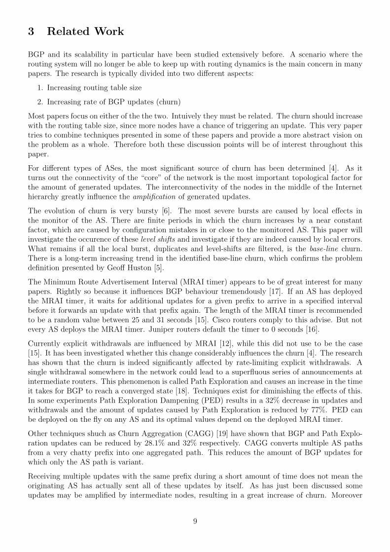
Figure 1 portrays the unstability of the signal. There are a numerous distinct peaks in the graph.Interestingly the high peaks started appearing halfway through 2008, are very prevalent during 2009,relatively quiet during 2010 and the beginning of 2011 and suddenly very frequent in 2013. Thesepeaks may be the consequence of a hard BGP session resets, in which BGP speakers exchange theirentire routing table with each other and RRC00. Failing data collectors contribute between 14% to37% of the total session resets. Moreover a session reset is necessary in order to allow policy changesto take into effect. At the end of 2013, the amount of entries in the BGP routing table reachesnearly 500,000 [2]. Surprisingly the peaks in Figure 1 can be a factor 1.2 × 102 higher than that.Apparently the BGP table can be loaded many times on a single day. This is all part of normal BGPoperations. Investigating these peaks is not that relevant for now, since we are looking for actualtrends. Furthermore it can be seen that the minimum amount of updates stays relatively stable untilhalfway through 2011, after which it rises to a new plateau. In 2012 and 2013 the rate does not reachthe usual minimum as seen from 2005 to 2011.

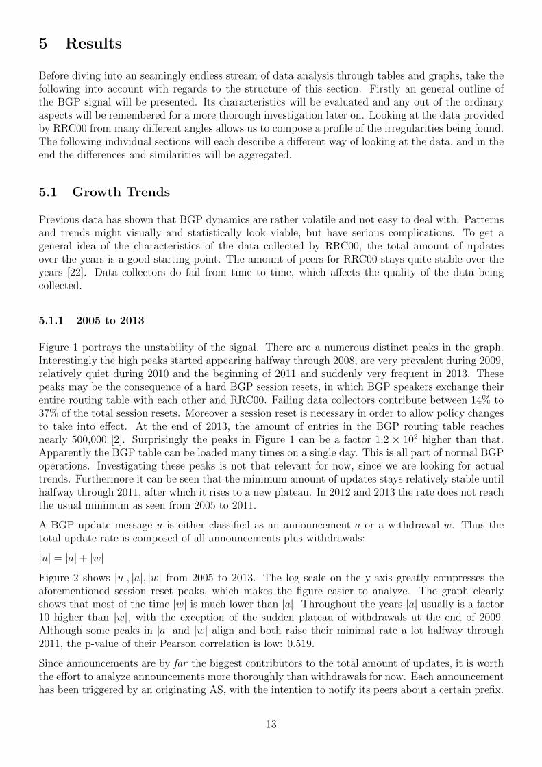
A BGP update message u is either classified as an announcement a or a withdrawal w. Thus thetotal update rate is composed of all announcements plus withdrawals:

|u| = |a|+ |w|

Figure 2 shows |u|, |a|, |w| from 2005 to 2013. The log scale on the y-axis greatly compresses theaforementioned session reset peaks, which makes the figure easier to analyze. The graph clearlyshows that most of the time |w| is much lower than |a|. Throughout the years |a| usually is a factor10 higher than |w|, with the exception of the sudden plateau of withdrawals at the end of 2009.Although some peaks in |a| and |w| align and both raise their minimal rate a lot halfway through2011, the p-value of their Pearson correlation is low: 0.519.

Since announcements are by far the biggest contributors to the total amount of updates, it is worththe effort to analyze announcements more thoroughly than withdrawals for now. Each announcementhas been triggered by an originating AS, with the intention to notify its peers about a certain prefix.

13

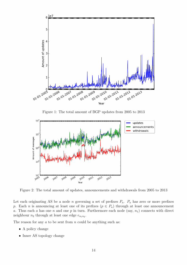
Figure 1: The total amount of BGP updates from 2005 to 2013

Figure 2: The total amount of updates, announcements and withdrawals from 2005 to 2013

Let each originating AS be a node n governing a set of prefixes Pn. Pn has zero or more prefixesp. Each n is announcing at least one of its prefixes (p ∈ Pn) through at least one announcementa. Thus each a has one n and one p in turn. Furthermore each node (say, n1) connects with directneighbour n2 through at least one edge en1n2 .

The reason for any a to be sent from n could be anything such as:

• A policy change

• Inner AS topology change

14

• A broken physical link to a peer initiated by a withdrawal

From an announcement alone it is often hard to derive what the exact cause was for it to be send.After an a has been sent, it traverses the Internet until it reaches the monitor of RRC00. Consequentlythis could mean that the amount of announcements an originating AS sends is proportional to theamount of prefixes it has.

|∀a(origin = n)| ∝ |p ∈ Pn|

Assuming every prefix is equally stable, this means there is a correlation between the amount ofcollected announcements and the amount of advertised prefixes. Whether or not every prefix isequally stable will be investigated later in this paper.

Figure 3: The amount of daily announced prefixes from 2005 to 2013

Figure 3 shows the aggregated |p| from all nodes from 2005 to 2013. It looks like there is an upperlimit that grows by a constant factor every day. Each year around unique 40,000 new prefixes areseen in BGP announcements. This matches the size and growth of the BGP table produced byGeoff Huston[2]. There are many days in which only a smalller portion of this upper limit is beingannounced. Halfway through 2011 the growth factor of this upper limit suddenly increases. Thiscould be explained by the exhaustion of the IPv4 address space [2]. Furthermore in the last half of2013 there is only one valley. This is remarkable given the high amount of valleys in the previousyears. This means that in 2013 nearly all prefixes in the routing table are announced every day.

If |p| influences |a|, then |n| and the amount of unique AS paths (|paths|) could potentially play arole in this as well. Figure 4 shows the rates for all four of them. All datasets show an increase innumbers over the years. The |p| and |n| show similar upper limit growth, while |a| and |paths| showsimilar volatile growth. The graph suggests a correlation between |p| and |n|, and between |a| and|paths|.

Indeed, Table 1 shows a very high correlation (0.995) between |p| and |n|. This makes sense becauseeach AS has a unique set of prefixes. Whenever an AS does not send any announcements on aparticular day, the prefixes it controls will not be registered by the collector either. If more ASes do

15

talk on such a day, the amount of collected prefixes will inevitably increase. Hence the correlationand a plausible causation of |p| and |n|.

Moreover the correlation between |a| and |paths| is also noticeably high (0.867). There is a possiblereason for this as well. The amount of |n| grows steadily over the years. Each AS has to advertiseat least one AS path, otherwise it would not be able to connect to the Internet. Consequently theamount of AS paths grows. If a new AS path is registered by the collector, it has to be transportedby at least one announcement. This reasoning derives the following statement for received updatesat any collector:

|n| < |paths| ∨ |p| < |a|

It should be remarked that there is a relatively low correlation between the amount of announce-ments and originating ASes (0.596). More talking ASes does not actually guarantee an increase inannouncements. Suppose there is a timeframe T with |n| = 10, from which one node sends thousandsand thousands of announcements. On T ′ the amount of nodes increases: |n| = 11, but they are allrelatively quiet, sending an average of 5 announcements. There is an increase in ASes, but a declinein announcements.

Announcements Prefixes Originating ASes AS PathsAnnouncements 1.000 0.616 0.596 0.867Prefixes 0.616 1.000 0.995 0.726Originating ASes 0.596 0.995 1.000 0.707AS Paths 0.867 0.726 0.707 1.000

Table 1: The p-values of the Pearson correlations between the amount of Announcements, Prefixes,Originating ASes and AS Paths

Figure 4: The amount of announcements, prefixes, as paths and originating ASes from 2005 to 2013

As seen in Figure 3, the amount of prefixes advertised in 2012 and 2013 does not exactly fit the lineof expectations: The growth rate looks predictable from 2005 to 2011, but takes a sudden steeperclimb starting 01-04-2011. This is surprising since the amount of originating ASes does grow in theway it would be expected. To investigate this deviation from the trend, lets take a closer look at theyear 2013.

16

(a) Prefix lower than 20 (b) Prefix between 20 and 24 (including)

Figure 5: Amount of prefixes from 2005 to 2013

5.1.2 2013

Although the difference is subtle, Figure 5 (a) and (b) show an asymmetry in growth over the years.Let the prefix (everything behind the slash) of a p be ps. Figure 5(a) shows that

|∀p(ps < 20)|

has the expected linear growth. On the other hand

|∀p(20 ≤ ps ≤ 24)|

shows the sudden “accelerated” growth as discussed in Section 5.1.1. Apparently there is an addi-tional increase in more specific prefixes starting from 01-04-2011, while the amount of more generalprefixes does not have this boost. Again, the exhaustion of IPv4 addresses is held responsible for thisbehaviour. A more thorough analysis for the increase in specific prefixes is not in the scope of thispaper. It is advised to keep an eye on this for the future though, as yet another boost of the specificscould greatly increase the amount of prefixes (and thus probably the amount of announcements aswell) to be advertised on the Internet again.

5.2 Top Talkers

Given the unstable signal of the BGP update messages rate, it is highly unlikely that every n has(nearly) the same amount of updates per day. When a particular node is route flapping, updates aresend on a regular (predictable) interval. Other nodes might be situated in a very stable setting, inwhich there should not be much reason to talk all the time. For the nodes which do talk a lot, it isinteresting to assess their combined daily rate of updates. There could be a set of nodes accountingfor a substantial portion of the total amount of updates. Determining their share of the total ratecould give more insights into the dynamics of BGP.

5.2.1 Top Talking Peers

By analyzing all the updates and keeping track of the last AS in the AS path, a list of top talkingpeers can be constructed. Table 2 shows a comparison of the top 10 of peers in the first half of2013.

17

January February March April May June01. 3549 3549 29049 29049 9304 930402. 9304 29049 15469 9304 29049 1546903. 1836 22652 3549 3549 3549 354904. 3333 3333 57821 3333 50300 2904905. 42109 15469 3333 15469 15469 333306. 29049 8758 7018 7018 3333 701807. 22652 57821 50304 8758 7018 875808. 57821 9304 9304 57821 8758 2265209. 8758 7018 8758 57381 57821 5030010. 7018 50300 22652 22652 22652 6881total 64.49% 61.84% 65.05% 71.89% 80.40% 69.82%

Table 2: A list of the top 10 talking peer ASes over the first four months of 2013 and the totalpercentage of the rate they contribute

Out of the 43 ASes peered to RRC00, there is a fairly constant set of peers that make it to the top10 talkers. There are 9 of these ASes in the top 10 for at least 5 out of the 6 months. The bottomrow shows the aggregate percentage of these ASes of the total amount of updates per month. Itshould be noted that these percentages are rather high, especially for May. Although the aggregatepercentages differ a lot per month, the set of top talkers does not change much. So this dataquantifies the importance of a certain subset of peers to RRC00 regardless of the time of the yearand the amount of updates being collected.

The sudden increase of aggregated percentages for the month of May is remarkable. AS number3549 has been forced two places downwards, while ASes 9304 and 29049 take over the first andsecond ranks. By looking at the contributed share of each individual AS, 9304 takes a very highpercentage (34.51%) of the total rate in May. It continues to do so, albeit to lesser exent, duringJune (22.86%). When aggregating the individual AS percentages over all the months, AS9304 comesout as a clear winner (16.45%) followed by AS29049 (10.25%) and AS3549 (9.08%). These threeASes can be classified as the most important peer contributors. The amount of updates these peerstake care of over course of time is shown in Figure 6. The way these three ASes take their place inTable 2 is also reflected in Figure 6:

1. AS9304 peaks around 21-01-2013, which gives it a high rank in January. It stays relatively quietuntil the second half of April after which it climbs to an elevated plateau and stays there forthe whole of May and most of June. Correspondingly the table gives it a number one rankingas well.

2. AS29049 builds up to and peaks in March and April, after which it stays around the same levelas AS3549 but is considerably overruled by AS9304. Indeed, according to the table AS29049slowly builds up to peak in March and April, and cools down afterwards.

3. AS3549 used to be a top talker according to the figure, but is quickly pushed downwards byAS9304 and AS29049. However it does stay in the top 3 all the time, which makes it morestable when comparing to the rest.

The irregular behaviour seen in May sparks some interest. It is interesting to investigate the suddenelevated plateau caused by peer AS9304.

18

Figure 6: The rate of updates from peers 9304, 29049 and 3549 from January to July 2013

5.2.2 Top Talking Originating ASes

The fact that AS9304 shows this unusual plateau does not tell anything about the cause of it. AS9304is merely the peer, the last AS in the AS path before it is collected by RRC00. It does not actuallygenerate the announcement itself. In order to find out more about the exact cause of this behaviourin May, it is of even more interest to look at the origin of AS paths. These nodes send out theoriginal announcement and will thus give a more detailed view of the announcements’ behaviour.Before looking at the data, it should be remarked that there are currently around 46280 ASes [2].Therefore the total amount of updates is spread over many more originating nodes than it is overpeers. Consequently the top talking originating nodes will probably have a much lower percentageof the total rate than peers. Table 3 confirms this believe by showing that the top 10 originatingASes only amounts to 8.04% compared to more than 60% for the top 10 peers.

The second column in Table 3 (Peer(s)) identifies the possible peers from which the announcementsmight be collected by RRC00. These sets of peers are retrieved using the following method:

1. Generate a top 100 list of AS paths through which the most announcements flowed

2. For each originating AS in the top 10, cross reference them with the orginating ASes in the top100 of AS paths

3. Traverse the AS path from right to left and mark the corresponding peer

As can be seen from these sets, the algorithm produces many peers for some originating ASes, whileothers do not have any at all. If such an AS only has one peer, the greatest share of announcementshave been going through that particular peer before reaching the collector. If the amount of peersis high, the announcements have been spread out over many paths before reaching the collector. Ifthere is no peer, it means the AS paths of the originating AS just were not used enough for them toappear in the top 100 AS paths. Since the originating AS did send many packets though, it probably

19

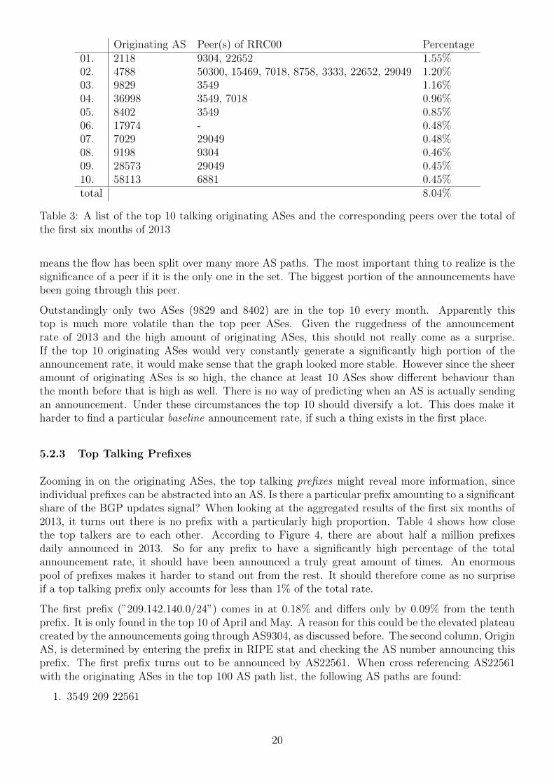
Originating AS Peer(s) of RRC00 Percentage01. 2118 9304, 22652 1.55%02. 4788 50300, 15469, 7018, 8758, 3333, 22652, 29049 1.20%03. 9829 3549 1.16%04. 36998 3549, 7018 0.96%05. 8402 3549 0.85%06. 17974 - 0.48%07. 7029 29049 0.48%08. 9198 9304 0.46%09. 28573 29049 0.45%10. 58113 6881 0.45%total 8.04%

Table 3: A list of the top 10 talking originating ASes and the corresponding peers over the total ofthe first six months of 2013

means the flow has been split over many more AS paths. The most important thing to realize is thesignificance of a peer if it is the only one in the set. The biggest portion of the announcements havebeen going through this peer.

Outstandingly only two ASes (9829 and 8402) are in the top 10 every month. Apparently thistop is much more volatile than the top peer ASes. Given the ruggedness of the announcementrate of 2013 and the high amount of originating ASes, this should not really come as a surprise.If the top 10 originating ASes would very constantly generate a significantly high portion of theannouncement rate, it would make sense that the graph looked more stable. However since the sheeramount of originating ASes is so high, the chance at least 10 ASes show different behaviour thanthe month before that is high as well. There is no way of predicting when an AS is actually sendingan announcement. Under these circumstances the top 10 should diversify a lot. This does make itharder to find a particular baseline announcement rate, if such a thing exists in the first place.

5.2.3 Top Talking Prefixes

Zooming in on the originating ASes, the top talking prefixes might reveal more information, sinceindividual prefixes can be abstracted into an AS. Is there a particular prefix amounting to a significantshare of the BGP updates signal? When looking at the aggregated results of the first six months of2013, it turns out there is no prefix with a particularly high proportion. Table 4 shows how closethe top talkers are to each other. According to Figure 4, there are about half a million prefixesdaily announced in 2013. So for any prefix to have a significantly high percentage of the totalannouncement rate, it should have been announced a truly great amount of times. An enormouspool of prefixes makes it harder to stand out from the rest. It should therefore come as no surpriseif a top talking prefix only accounts for less than 1% of the total rate.

The first prefix (”209.142.140.0/24”) comes in at 0.18% and differs only by 0.09% from the tenthprefix. It is only found in the top 10 of April and May. A reason for this could be the elevated plateaucreated by the announcements going through AS9304, as discussed before. The second column, OriginAS, is determined by entering the prefix in RIPE stat and checking the AS number announcing thisprefix. The first prefix turns out to be announced by AS22561. When cross referencing AS22561with the originating ASes in the top 100 AS path list, the following AS paths are found:

1. 3549 209 22561

20

2. 7018 209 22561

3. 9304 2914 209 22561

The third AS path confirms the assumption that there is a path from 22561 through 9304 to thecollector. It does not give full assurance the prefix (”209.142.140.0/24”) is part of the explanation ofthe elevated plateau yet. The prefix could also be flowing for the biggest part through the first ASpath in the list, thereby falsifying the assumption. Later on this matter will be investigated in moredetail.

Moving on, the second prefix (”208.78.30.0/24”) is found in every month except March. Do noteMarch has a very high peak in the middle, which is associated with session resets from peers of thecollector. Therefore in March the top 10 prefixes might seem to be little off, since the entire routingtable had to be exchanged between several ASes. According to Figure 6, the increase of informationbeing exchanged during this reset is aproximately a factor 10.

Prefix Origin AS Percentage01. 209.142.140.0/24 22561 0.18%02. 208.78.30.0/24 29838 0.16%03. 192.58.232.0/24 6629 0.15%04. 2a00:1a80::/32 33920 0.15%05. 208.68.168.0/21 29838 0.15%06. 199.188.67.0/24 393238 0.11%07. 58.184.229.0/24 9950 0.10%08. 2001:df0:2fd::/48 17436 0.10%09. 184.159.130.0/23 22561 0.09%10. 115.170.128.0/17 4847 0.09%total 1.28%

Table 4: A list of the top 10 talking prefixes over the total of the first six months of 2013

If the set of top talking peers, originating ASes and prefixes changes so much in a couple of monthsin 2013, how does the set hold over a couple of years?

5.2.4 2005-2013

Given the diversity of the top talkers every month, it would not be sensible to assume the set wouldbe more constant over a few years. In fact, very few ASes and prefixes appear in the top on a regularbasis.

The evidence that the composition of the top talkers varies a lot over the years, opens up a newdiscussion. The set of ASes and prefixes is so vast, that finding patterns in a small subset is perhapsnot very practical. New ways have to be found to look at the dynamics of BGP as a whole. Inessence the granular approach used in this section does not give sufficient insight. Top talkers arejust the tip of the iceberg. What lies underneath it may have a significant influence on the updaterate of BGP.

5.3 Distributions of updates

To combat the problem of subsets being to small to properly analyze, a logical step would be to lookat the BGP update rate as a whole. From 2005 to 2013 the rate looks very jagged. Upon closer

21

inspection of the ASes and prefixes that contributed the most to the overall rate, the set of toptalkers looks variable. By taking all nodes into consideration, not only top talkers, groups of ASesor prefixes sharing a certain set of properties or actions may be found. After all a group of ASes orprefixes (a cluster) may not necessarily just be top talkers. There are many other possible commonaspects to focus on, like timestamps, AS paths and community information. To get a general ideaof the way a population of nodes behaves, plotting update distributions will give valuable insights.Since every BGP update is in some way included in such a distribution, it will portray a general yetrich in information projection of reality.

Let the set of all originating ASes be Sorig and the set of all prefixes be Spref . A node n ∈ Sorig existsif it has sent an announcement at least one time. Each announcement has a timestamp t. The settn consists of all the timestamps t of node n and similarly the set tp consists of all the t of prefixp.

n ∈ Sorigp ∈ Spreftn 6= ∅ tp 6= ∅

Say there is a timeframe T (e.g. 18 January 2013). A node is active in a timeframe if it has sentat least one announcement during the timeframe. Let Tn and Tp be the set of all active nodes andprefixes respectively in timeframe T .

∀n ∈ Tn(∃t ∈ (tn ∩ T ))

∀n ∈ Tp(∃t ∈ (tp ∩ T ))

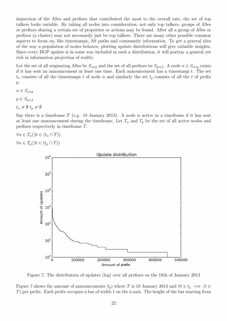
Figure 7: The distribution of updates (log) over all prefixes on the 18th of January 2013

Figure 7 shows the amount of announcements |tp| where T is 18 January 2013 and ∀t ∈ tp =⇒ (t ∈T ) per prefix. Each prefix occupies a bar of width 1 on the x-axis. The height of the bar starting from

22

(a) Amount of prefixes (b) Amount days

Figure 8: Distributions of prefixes in the month January 2013

the x-axis is determined by |tp|. The entire set of prefixes is sorted from high to low according to theamount of updates and then plotted on the graph. Therefore distribution shows the top talkers onthe far left and the quieter ones on the far right. Clearly a great amount of prefixes only announcea small amount of updates. For 94.34% of the prefixes |tp| <= 50 holds. The surface underneaththe graph determines the total amount of announcements that have been sent. The prefixes withless than or equal to 50 announcements contribute 34.91% to the overall announcement rate. Thismeans there is a small (5.66%) subset of Tp which sends a substantial portion (65.09%) of the totalannouncement rate.

As observed in the list of top talkers, BGP behaviour can change when looking at larger timeframes.Let T ′ be the month January in 2013. A prefix p ∈ Spref is active on a day if that prefix has atimestamp on that particular day. Let Dp be the set of days a prefix is active.

The curve of the graph in Figure 8(a) looks different from curve of Figure 7. Again there is a smallset of top talkers and the curve smoothly advances to a plateau, around tp = 10. The last part ofthe curve drops remarkably quick to the absolute minimum of tp = 0. The sudden drop after theplateau is unusual. When comparing the distribution of |tp| to the distribution of |Dp|, the curveshows a similar pattern. The plateau is located around |Dp = 20|. Thus most prefixes are activefor at least 20 days per month. After the plateau the curve goes to the minimum of |Dp = 1| verysteeply. A more detailed look at the data shows that the set of prefixes in the tp and the Dp plateausare corresponding. Similarly the set of prefixes with Dp < 20 corresponds to the set of prefixes withtp < 200. This means there is a distinct set of prefixes which does not talk as much and as regularas the rest. This set will be analyzed in detail later on.

Now remember the elevated plateau in Figure 6 caused by peer AS9304. Such irregular behaviourshould also be noticeable in the distributions of tp and Dp. When plotting the distribution of tp, anew small plateau is observed just above tp = 10, 000. This is in contrast to the curve in January2013, which totally lacks this plateau.

Presumably the new plateau is caused by the set of nodes with announcements going through peerAS9304. Since the root cause of this plateau is not yet exactly known, AS9304 cannot yet becharacterized as the main link for this plateau as well. In section 5.5.5 the set of originating ASesassociated with this pattern will be determined. It should be noted that this new plateau is not in anyway visible when plotting the amount of updates per node (originating AS). Apparently quantifying

23

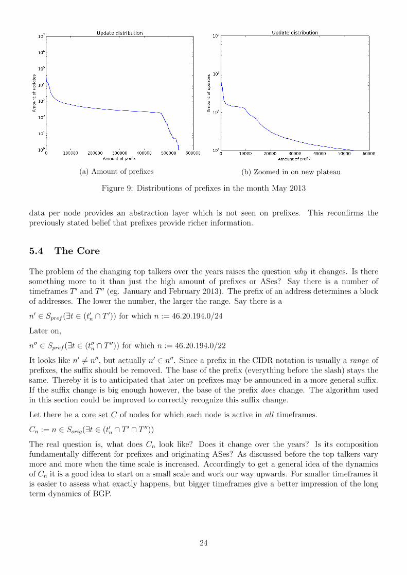
(a) Amount of prefixes (b) Zoomed in on new plateau

Figure 9: Distributions of prefixes in the month May 2013

data per node provides an abstraction layer which is not seen on prefixes. This reconfirms thepreviously stated belief that prefixes provide richer information.

5.4 The Core

The problem of the changing top talkers over the years raises the question why it changes. Is theresomething more to it than just the high amount of prefixes or ASes? Say there is a number oftimeframes T ′ and T ′′ (eg. January and February 2013). The prefix of an address determines a blockof addresses. The lower the number, the larger the range. Say there is a

n′ ∈ Spref (∃t ∈ (t′n ∩ T ′)) for which n := 46.20.194.0/24

Later on,

n′′ ∈ Spref (∃t ∈ (t′′n ∩ T ′′)) for which n := 46.20.194.0/22

It looks like n′ 6= n′′, but actually n′ ∈ n′′. Since a prefix in the CIDR notation is usually a range ofprefixes, the suffix should be removed. The base of the prefix (everything before the slash) stays thesame. Thereby it is to anticipated that later on prefixes may be announced in a more general suffix.If the suffix change is big enough however, the base of the prefix does change. The algorithm usedin this section could be improved to correctly recognize this suffix change.

Let there be a core set C of nodes for which each node is active in all timeframes.

Cn := n ∈ Sorig(∃t ∈ (t′n ∩ T ′ ∩ T ′′))

The real question is, what does Cn look like? Does it change over the years? Is its compositionfundamentally different for prefixes and originating ASes? As discussed before the top talkers varymore and more when the time scale is increased. Accordingly to get a general idea of the dynamicsof Cn it is a good idea to start on a small scale and work our way upwards. For smaller timeframes itis easier to assess what exactly happens, but bigger timeframes give a better impression of the longterm dynamics of BGP.

24

Figure 10: The rate of announcements, prefixes and originating ASes in January 2013

(a) Per originating AS (b) Per prefix

Figure 11: The distribution of differences in core updates (log) from 18 to 19 January

5.4.1 Days

To analyse such a small timeframe, lets find two days that have approximately equal amounts ofactive nodes and total updates. Figure 10 shows a relatively stable period from the 15th to the 22ndof January 2013. The amount of prefixes and originating ASes barely changes during that time whilethe announcements vary slightly more. Although the 18th and 19th of January have nearly the sameamount of announcements as well. Lets focus on those two days for now and see if it is really asstable as it looks.

The distributions in Figure 11 show the difference in updates from 18 to 19 January. Each prefix(Figure a) or AS (Figure b) occupies a bar of width 1 on the x-axis. The height of the bar from the0-line is determined by the difference in amount of updates. Say the node has sent 20 announcementsduring the first timeframe and 90 during the second, the height would be 70. A negative differencewould result in the bar being flipped over the x-axis. Let δn be the absolute value of the growth ofa node. Thus the surface below the graph represents the total change in core announcements. Theentire set of nodes is sorted from high to low according to their difference and then plotted on the

25

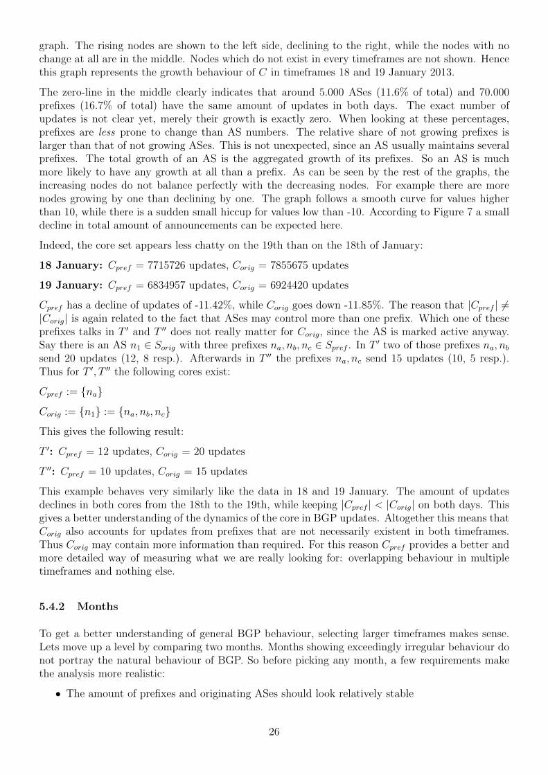
graph. The rising nodes are shown to the left side, declining to the right, while the nodes with nochange at all are in the middle. Nodes which do not exist in every timeframes are not shown. Hencethis graph represents the growth behaviour of C in timeframes 18 and 19 January 2013.

The zero-line in the middle clearly indicates that around 5.000 ASes (11.6% of total) and 70.000prefixes (16.7% of total) have the same amount of updates in both days. The exact number ofupdates is not clear yet, merely their growth is exactly zero. When looking at these percentages,prefixes are less prone to change than AS numbers. The relative share of not growing prefixes islarger than that of not growing ASes. This is not unexpected, since an AS usually maintains severalprefixes. The total growth of an AS is the aggregated growth of its prefixes. So an AS is muchmore likely to have any growth at all than a prefix. As can be seen by the rest of the graphs, theincreasing nodes do not balance perfectly with the decreasing nodes. For example there are morenodes growing by one than declining by one. The graph follows a smooth curve for values higherthan 10, while there is a sudden small hiccup for values low than -10. According to Figure 7 a smalldecline in total amount of announcements can be expected here.

Indeed, the core set appears less chatty on the 19th than on the 18th of January:

18 January: Cpref = 7715726 updates, Corig = 7855675 updates

19 January: Cpref = 6834957 updates, Corig = 6924420 updates

Cpref has a decline of updates of -11.42%, while Corig goes down -11.85%. The reason that |Cpref | 6=|Corig| is again related to the fact that ASes may control more than one prefix. Which one of theseprefixes talks in T ′ and T ′′ does not really matter for Corig, since the AS is marked active anyway.Say there is an AS n1 ∈ Sorig with three prefixes na, nb, nc ∈ Spref . In T ′ two of those prefixes na, nbsend 20 updates (12, 8 resp.). Afterwards in T ′′ the prefixes na, nc send 15 updates (10, 5 resp.).Thus for T ′, T ′′ the following cores exist:

Cpref := {na}

Corig := {n1} := {na, nb, nc}

This gives the following result:

T ′: Cpref = 12 updates, Corig = 20 updates

T ′′: Cpref = 10 updates, Corig = 15 updates

This example behaves very similarly like the data in 18 and 19 January. The amount of updatesdeclines in both cores from the 18th to the 19th, while keeping |Cpref | < |Corig| on both days. Thisgives a better understanding of the dynamics of the core in BGP updates. Altogether this means thatCorig also accounts for updates from prefixes that are not necessarily existent in both timeframes.Thus Corig may contain more information than required. For this reason Cpref provides a better andmore detailed way of measuring what we are really looking for: overlapping behaviour in multipletimeframes and nothing else.

5.4.2 Months

To get a better understanding of general BGP behaviour, selecting larger timeframes makes sense.Lets move up a level by comparing two months. Months showing exceedingly irregular behaviour donot portray the natural behaviour of BGP. So before picking any month, a few requirements makethe analysis more realistic:

• The amount of prefixes and originating ASes should look relatively stable

26

• There should be no factor 10 peaks

• There should be no continual high volume elevated plateaus over an extended period of time

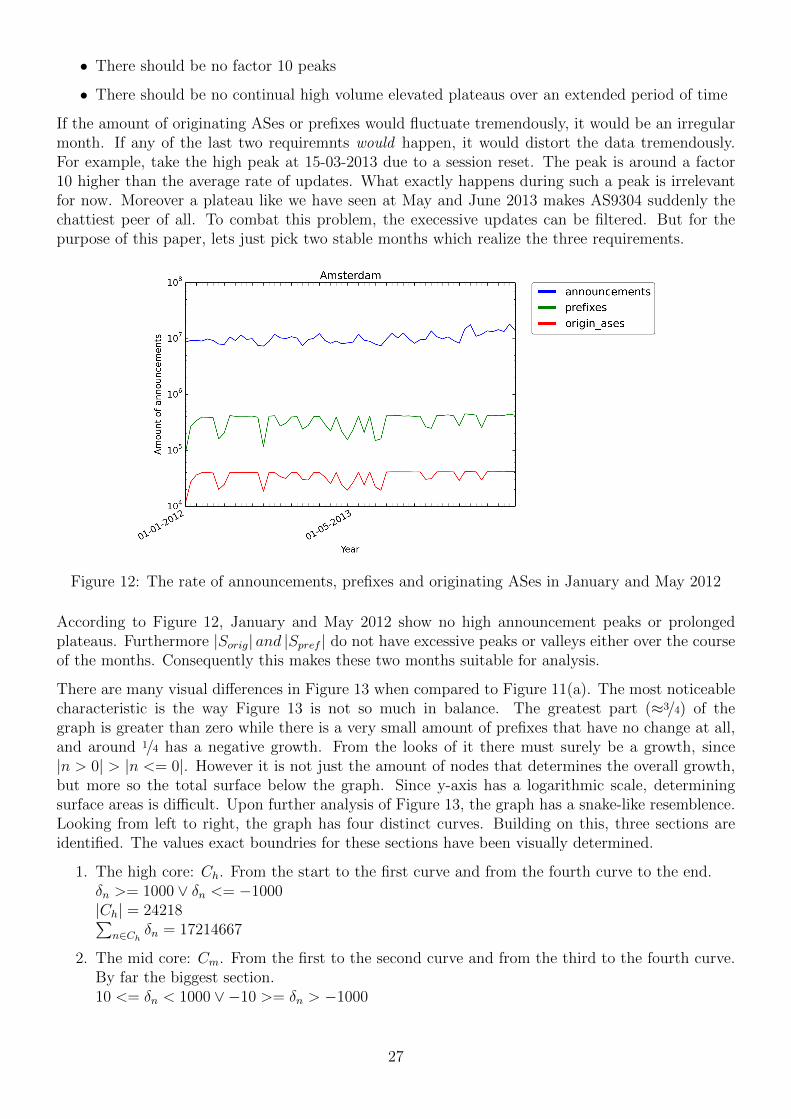
If the amount of originating ASes or prefixes would fluctuate tremendously, it would be an irregularmonth. If any of the last two requiremnts would happen, it would distort the data tremendously.For example, take the high peak at 15-03-2013 due to a session reset. The peak is around a factor10 higher than the average rate of updates. What exactly happens during such a peak is irrelevantfor now. Moreover a plateau like we have seen at May and June 2013 makes AS9304 suddenly thechattiest peer of all. To combat this problem, the execessive updates can be filtered. But for thepurpose of this paper, lets just pick two stable months which realize the three requirements.

Figure 12: The rate of announcements, prefixes and originating ASes in January and May 2012

According to Figure 12, January and May 2012 show no high announcement peaks or prolongedplateaus. Furthermore |Sorig| and |Spref | do not have excessive peaks or valleys either over the courseof the months. Consequently this makes these two months suitable for analysis.

There are many visual differences in Figure 13 when compared to Figure 11(a). The most noticeablecharacteristic is the way Figure 13 is not so much in balance. The greatest part (≈3/4) of thegraph is greater than zero while there is a very small amount of prefixes that have no change at all,and around 1/4 has a negative growth. From the looks of it there must surely be a growth, since|n > 0| > |n <= 0|. However it is not just the amount of nodes that determines the overall growth,but more so the total surface below the graph. Since y-axis has a logarithmic scale, determiningsurface areas is difficult. Upon further analysis of Figure 13, the graph has a snake-like resemblence.Looking from left to right, the graph has four distinct curves. Building on this, three sections areidentified. The values exact boundries for these sections have been visually determined.

1. The high core: Ch. From the start to the first curve and from the fourth curve to the end.δn >= 1000 ∨ δn <= −1000|Ch| = 24218∑

n∈Chδn = 17214667

2. The mid core: Cm. From the first to the second curve and from the third to the fourth curve.By far the biggest section.10 <= δn < 1000 ∨ −10 >= δn > −1000

27

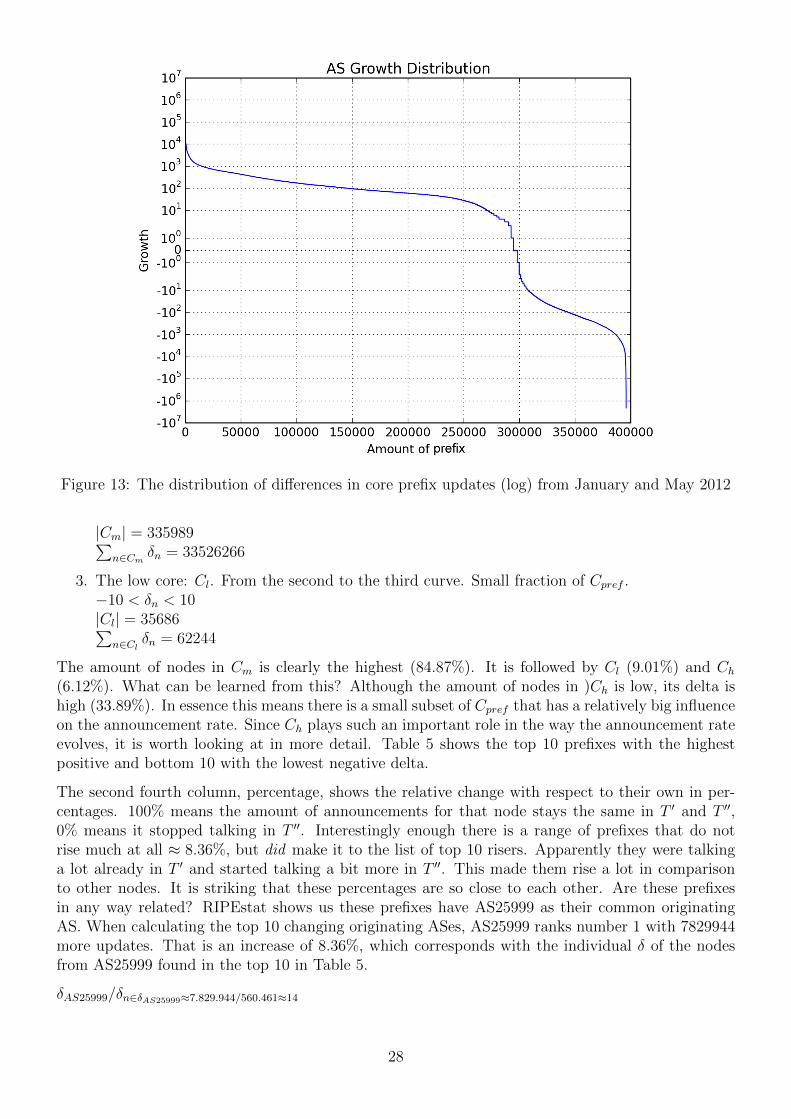
Figure 13: The distribution of differences in core prefix updates (log) from January and May 2012

|Cm| = 335989∑n∈Cm

δn = 33526266

3. The low core: Cl. From the second to the third curve. Small fraction of Cpref .−10 < δn < 10|Cl| = 35686∑

n∈Clδn = 62244

The amount of nodes in Cm is clearly the highest (84.87%). It is followed by Cl (9.01%) and Ch(6.12%). What can be learned from this? Although the amount of nodes in )Ch is low, its delta ishigh (33.89%). In essence this means there is a small subset of Cpref that has a relatively big influenceon the announcement rate. Since Ch plays such an important role in the way the announcement rateevolves, it is worth looking at in more detail. Table 5 shows the top 10 prefixes with the highestpositive and bottom 10 with the lowest negative delta.

The second fourth column, percentage, shows the relative change with respect to their own in per-centages. 100% means the amount of announcements for that node stays the same in T ′ and T ′′,0% means it stopped talking in T ′′. Interestingly enough there is a range of prefixes that do notrise much at all ≈ 8.36%, but did make it to the list of top 10 risers. Apparently they were talkinga lot already in T ′ and started talking a bit more in T ′′. This made them rise a lot in comparisonto other nodes. It is striking that these percentages are so close to each other. Are these prefixesin any way related? RIPEstat shows us these prefixes have AS25999 as their common originatingAS. When calculating the top 10 changing originating ASes, AS25999 ranks number 1 with 7829944more updates. That is an increase of 8.36%, which corresponds with the individual δ of the nodesfrom AS25999 found in the top 10 in Table 5.

δAS25999/δn∈δAS25999≈7.829.944/560.461≈14

28

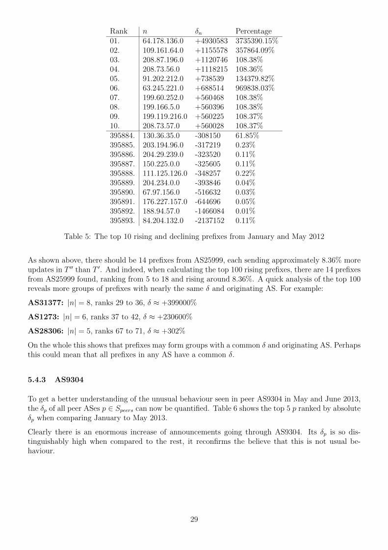
Rank n δn Percentage01. 64.178.136.0 +4930583 3735390.15%02. 109.161.64.0 +1155578 357864.09%03. 208.87.196.0 +1120746 108.38%04. 208.73.56.0 +1118215 108.36%05. 91.202.212.0 +738539 134379.82%06. 63.245.221.0 +688514 969838.03%07. 199.60.252.0 +560468 108.38%08. 199.166.5.0 +560396 108.38%09. 199.119.216.0 +560225 108.37%10. 208.73.57.0 +560028 108.37%395884. 130.36.35.0 -308150 61.85%395885. 203.194.96.0 -317219 0.23%395886. 204.29.239.0 -323520 0.11%395887. 150.225.0.0 -325605 0.11%395888. 111.125.126.0 -348257 0.22%395889. 204.234.0.0 -393846 0.04%395890. 67.97.156.0 -516632 0.03%395891. 176.227.157.0 -644696 0.05%395892. 188.94.57.0 -1466084 0.01%395893. 84.204.132.0 -2137152 0.11%

Table 5: The top 10 rising and declining prefixes from January and May 2012

As shown above, there should be 14 prefixes from AS25999, each sending approximately 8.36% moreupdates in T ′′ than T ′. And indeed, when calculating the top 100 rising prefixes, there are 14 prefixesfrom AS25999 found, ranking from 5 to 18 and rising around 8.36%. A quick analysis of the top 100reveals more groups of prefixes with nearly the same δ and originating AS. For example:

AS31377: |n| = 8, ranks 29 to 36, δ ≈ +399000%

AS1273: |n| = 6, ranks 37 to 42, δ ≈ +230600%

AS28306: |n| = 5, ranks 67 to 71, δ ≈ +302%

On the whole this shows that prefixes may form groups with a common δ and originating AS. Perhapsthis could mean that all prefixes in any AS have a common δ.

5.4.3 AS9304

To get a better understanding of the unusual behaviour seen in peer AS9304 in May and June 2013,the δp of all peer ASes p ∈ Speers can now be quantified. Table 6 shows the top 5 p ranked by absoluteδp when comparing January to May 2013.

Clearly there is an enormous increase of announcements going through AS9304. Its δp is so dis-tinguishably high when compared to the rest, it reconfirms the believe that this is not usual be-haviour.

29

Rank p δp Percentage01. 9304 +148941191 999.65%02. 29049 +30750897 336.05%03. 15469 +17505464 427.50%04. 50300 +15144870 276.24%05. 7018 +10389719 215.95%

Table 6: The top 5 rising peer ASes from January and May 2013

5.4.4 Years

Up until now the analyzed timeframes were close to each other in time. By studying vast timeframesover the span of a few years, an improved picture of BGP trends may be realized. After all, moredata over a longer period of time results in a more relevant perspective when analyzing trends. LetT ′ be the months January, May and September from the years 2005 and 2006. T ′′ has the samemonths, but from years 2010 and 2011. By taking more months and increasing the difference inyears between T ′ and T ′′ the resulting graph looks different than before. Figure 15 clearly showsthat the biggest portion of nodes actually decreases in amount of updates. This is surprising becauseaccording to Figure 4 the total amount updates should be growing over the years. Moreover the sizeof Cpref is noteworthy:

|Cpref | = 162029

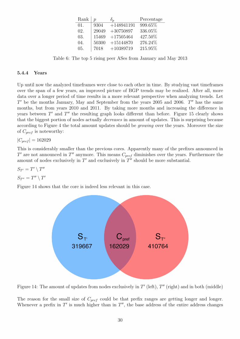
This is considerably smaller than the previous cores. Apparently many of the prefixes announced inT ′ are not announced in T ′′ anymore. This means Cpref diminishes over the years. Furthermore theamount of nodes exclusively in T ′ and exclusively in T ′′ should be more substantial.

ST ′ = T ′ \ T ′′

ST ′′ = T ′′ \ T ′

Figure 14 shows that the core is indeed less relevant in this case.

Figure 14: The amount of updates from nodes exclusively in T ′ (left), T ′′ (right) and in both (middle)

The reason for the small size of Cpref could be that prefix ranges are getting longer and longer.Whenever a prefix in T ′ is much higher than in T ′′, the base address of the entire address changes

30

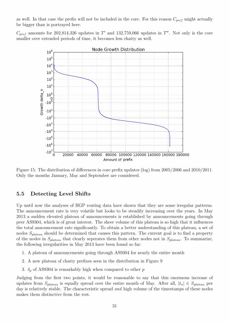
as well. In that case the prefix will not be included in the core. For this reason Cpref might actuallybe bigger than is portrayed here.

Cpref amounts for 202,814,326 updates in T ′ and 132,759,066 updates in T ′′. Not only is the coresmaller over extended periods of time, it becomes less chatty as well.

Figure 15: The distribution of differences in core prefix updates (log) from 2005/2006 and 2010/2011.Only the months January, May and September are considered.

5.5 Detecting Level Shifts

Up until now the analyses of BGP routing data have shown that they are some irregular patterns.The announcement rate is very volatile but looks to be steadily increasing over the years. In May2013 a sudden elevated plateau of announcements is established by announcements going throughpeer AS9304, which is of great interest. The sheer volume of this plateau is so high that it influencesthe total announcement rate significantly. To obtain a better understanding of this plateau, a set ofnodes Splateau should be determined that causes this pattern. The current goal is to find a propertyof the nodes in Splateau that clearly seperates them from other nodes not in Splateau. To summarize,the following irregularities in May 2013 have been found so far:

1. A plateau of announcements going through AS9304 for nearly the entire month

2. A new plateau of chatty prefixes seen in the distribution in Figure 9

3. δp of AS9304 is remarkably high when compared to other p

Judging from the first two points, it would be reasonable to say that this enormous increase ofupdates from Splateau is equally spread over the entire month of May. After all, |tn| ∈ Splateau perday is relatively stable. The characteristic spread and high volume of the timestamps of these nodesmakes them distinctive from the rest.

31

5.5.1 Burstiness

The spread of the timestamps of a node can be quantified using a measure of burstiness. First, letscreate a formal definition of burstiness

Burstiness: A burst βn ⊂ tn is a group of consecutive timestamps with shorter gaps in time thantimestamps before or after the burst.

A node is not bursty if its timestamps are fairly regular spaced out and do not depend on each other(Poisson). Finding a way to measure the exact burstiness of a node is not so trivial [24]. For now itsuffices to find an simpler heuristic, since we are only interested in finding a distinctive property ofSplateau. Say there is a node n with timestamps

tn = {0, 1, 2, 3, 10, 11, 12, 13, 20, 21, 22, 23}

By the definition of burstiness there clearly are three bursts. Let the time between two timestampst1 and t2 be the interval

it1t2 = t2 − t1The set of bursts in tn of consecutive timestamps is I with mean µI .

1. β′n = {0, 1, 2, 3}, µI = 1

2. β′′n = {10, 11, 12, 13}, µI = 1

3. β′′′n = {20, 21, 22, 23}, µI = 1

Now the simplest way to measure burstiness would be to count all the itxtx+1 < y for some appro-priately small y. However it is not known beforehand what such an y would be. For now it is toocomplicated to calculate y for all n ∈ Spref . In the example of three bursts, the µI of tn = 2.09.All of the values in I differ from µI . Say the intervals between bursts would be longer, µI would behigher, and the summed difference between each individual interval and µI would be even bigger.Furthermore if some tx+1 is appended to βn and itxtx+1

< µI , then the summed difference betweeneach interval and µI would again be bigger. In both cases the burstiness and the summed differencebetween each interval and µI increases.

Now say there is a node n2 with:

tn2 = {0, 5, 10, 15, 20, 25}

There are no actual bursts in tn2 because there are no consecutive timestamps with intervals lowerthan the timestamps before and after that. This means t2 is not bursty at all. µI for t2 is exactly 5and the summed difference between each interval and µI is exactly 0.

The repeated notion of summed differences between each interval and µI can be captured in thevariance of I. In essence this means the burstiness is correlated to the variance of the intervalsvar(I).

5.5.2 Plotting Variance

Figure 16 reveals a lot of new information. Both figures represent a projection of the same dataset.Each dot in Figure 16(a) expresses a node, or more specifically in this case, a prefix. Firstly, the setof intervals In for each node n on 03-06-2013 is worked out. Afterwards all the individual var(In)can be calculated. Secondly, count the amount of updates per node. Each node (x, y) is plotted onthe graph according to (var(In), |tn|). The color of each dot is determined by comparing the interval

32

(a) Including the activeness(b) Heatmap

Figure 16: The variance of intervals versus the amount of updates per node in 03-06-2013

Figure 17: Distribution updates over nodes on 03-06-2013

of the absolute first and absolute last timestamp of a node to the length of the day. Black meansit is active only for a very short period of time, while pink means the node started talking at 00:00and ended at 23:59. Previous figures have shown that the amount of nodes on a single day canbe tremendously high. Thus figure 16(a) has a potential visual shortcoming. There is a possibilitythat

∃n, n′ ∈ Spref (var(In) = var(In′) ∧ |tn| = |t′n|))

33

Consequently some nodes may overlap each other, since their coordinates are the same. That is whyfigure 16(b) is necessary to gain more insight in the density of areas of the graph. The spectrumfrom blue (low) to red (high) serves as a measurement of the amount of nodes in that particulararea.

5.5.3 Clusters

By looking at both Figure 16(a) and 16(b), several clusters can be distinguished.

1. The most straightforward of them all is the one in the lower left corner. This is the set of nodeswith only one timestamp, and thus a variance of zero. The red color on the heatmap showsthere is a fairly large portion of nodes in this area. This cluster is represented in Figure 17 onthe far right on the x-axis.

2. All nodes with 1 < |tn| < 10. The greatest amount of nodes in this cluster have two timestamps.Interestingly enough it looks like on average the variance is either ≈ 102 or ≈ 105. Moreoverthere are not many timestamps with a prolonged activeness.

3. On the lower left, centered around (10, 40), there is a cluster of nodes with a low variance andsmall amount of updates. The colors in this cluster range from black to slightly gray. Thusthe length of time these nodes are active is not so long. According to the green color on theheatmap the amount of nodes in this cluster is small. The most obvious section to link thiscluster to is the drop after the second plateau, as shown in Figure 9(a).

4. A bit to the right of the center of the graph there is a cluster of a pink nodes. Apparently thesenodes have a very long timespan since their pink color is so bright. Moreover the volume andvariance of these nodes is rather high.

5. There is a set of nodes with a low activeness like cluster 3, but with a higher variance.

6. There is a set of nodes with a high activeness and a high variance.

Every cluster except 4 is considered usual background noise. The composition (spread and volume)of these clusters changes per day, but they keep their distinctive characteristics. For example, cluster3 has days in which it is fairly round like in Figure 16(a). On other days the volume of nodes in thiscluster decreases by such a great amount, that the cluster is barely recognizable anymore. 03-06-2013has been picked as an example because the clusters are easily revealed here.

The cluster that is of great interest is 4, because it looks like it does not really belong there. It has aparticularly high volume of nodes when compared to the near surroundings in the graph. Furthermorethe bright pink color really sets it apart from the rest. This unusual cluster starts appearing nearthe end of April 2013 and disappears halfway June. Thus the timespan of this cluster coincides withthe elevated plateau of AS9304. Moreover the volume of cluster 3 makes it really chatty and likelyto have a high δ. In this case it fulfills three of the typical characteristics of Splateau as mentioned inSection 5.5. By determining all the nodes n ∈ Cluster4 it can be determined if Cluster4 ⊆ Splateau.Lets define three characteristics for all nodes n ∈ Cluster4 just by looking at Figure 16:

1. 104 < var(I) < 106

2. 102 < |tn| < 103

3. An > 0.95

34

(a) Amount of updates through AS9304 (b) Distribution of updates over nodes on 03-06-2013without Cluster4

Figure 18: Level shift in April, May and June 2013

5.5.4 Nodes causing the level shift

Using this short list of requirements the set of prefixes in Cluster4 can be generated. This setincludes 12181 prefixes. Proving Cluster4 ⊆ Splateau is troublesome because the nodes in Splateau arenot exactly known. For now only the (potential) visual effects of Splateau are known. Lets assumethe negation of Cluster4 ⊆ Splateau and find a contradiction.

As the first step in the proof by contradiction, let Cluster4 6⊆ Splateau. It is known that the updatesof all nodes in Splateau together form the characteristic structure of an elevated plateau. Accordingto the first assumption, the nodes in Cluster4 do not contribute anything to the appearance of theplateau, since the nodes in Cluster4 are not in Splateau. This means {Splateau \ Cluster4} = Splateau.Consequently by visualizing {Splateau \ Cluster4} the plateau should be unchanged.

As can clearly be seen in Figure 18(a), the plateau {Splateau \ Cluster4} much less recognizable andabout 5 times less chatty than Splateau by itself. Moreover Cluster4 shows a plateau very much likeSplateau does. However it has just been argued that Cluster4 would have no impact on the appearenceof the plateau at all. This contradiction falsifies the first assumption Cluster4 6⊆ Splateau. Not onlydoes Cluster4 contain nodes which are in Splateau, Cluster4 also has a considerable share in thecomposition of the plateau. This is because {Splateau \ Cluster4} does not deviate much from theaverage rate of updates going through AS9304. As a result this shows that

Cluster4 ≈ Splateau

Which is reinforced more so by the fact that the first new plateau has disappeared from the distri-bution of updates in Figure 18(b). Do note that the two sets cannot be exactly equal because bothof them have been determined by visually analyzing graphs. This leads to the following uncertain-ties:

1. The nodes in Splateau are not exactly known

2. The three characteristics defined for Cluster4 may leave out some nodes that are relevant

All things considered, the method above describes a way of detecting prolonged irregularities in theBGP signal. These level shifts are not part of the baseline of BGP but do contribute a significant

35

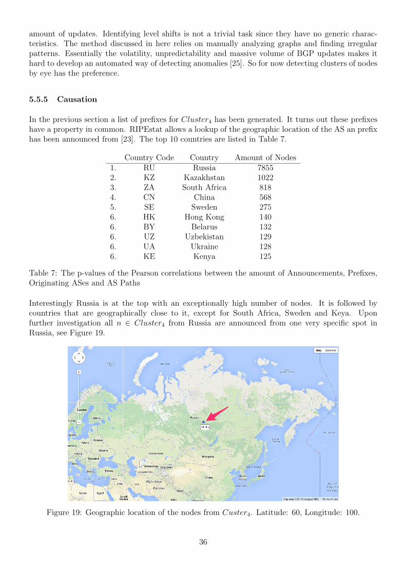
amount of updates. Identifying level shifts is not a trivial task since they have no generic charac-teristics. The method discussed in here relies on manually analyzing graphs and finding irregularpatterns. Essentially the volatility, unpredictability and massive volume of BGP updates makes ithard to develop an automated way of detecting anomalies [25]. So for now detecting clusters of nodesby eye has the preference.

5.5.5 Causation

In the previous section a list of prefixes for Cluster4 has been generated. It turns out these prefixeshave a property in common. RIPEstat allows a lookup of the geographic location of the AS an prefixhas been announced from [23]. The top 10 countries are listed in Table 7.

Country Code Country Amount of Nodes1. RU Russia 78552. KZ Kazakhstan 10223. ZA South Africa 8184. CN China 5685. SE Sweden 2756. HK Hong Kong 1406. BY Belarus 1326. UZ Uzbekistan 1296. UA Ukraine 1286. KE Kenya 125

Table 7: The p-values of the Pearson correlations between the amount of Announcements, Prefixes,Originating ASes and AS Paths

Interestingly Russia is at the top with an exceptionally high number of nodes. It is followed bycountries that are geographically close to it, except for South Africa, Sweden and Keya. Uponfurther investigation all n ∈ Cluster4 from Russia are announced from one very specific spot inRussia, see Figure 19.

Figure 19: Geographic location of the nodes from Custer4. Latitude: 60, Longitude: 100.

36

(a) 3 to 14 June 2013(b) 14 June 2013

Figure 20: Update growth per node versus amount of updates heatmap

The n from other countries close to Russia have paths going through this specific place in Russia aswell. This is checked using the following method:

1. Generate a list of all known AS paths in Cluster4

2. Generate a list of all originating AS paths in Cluster4 not from Russia

3. Crossreference both lists and check for each originating AS all the nodes for all its AS paths

4. If any of the nodes on the AS paths goes through that specific place in Russia, flag it

The fact that all the n ∈ Cluster4 originate from or have paths going through one specific spot inRussia, means the reason for the behaviour of Cluster4 can be attributed to this very place.

5.5.6 Other irregularities

Besides detecting level shifts, these steps can also detect other irregularities. For example, a levelshift with a vast amount of updates can be seen starting from the 14 to 27 June 2013. Lets callthe set of nodes causing this level shift Sx. As shown in Figure 20(a) the cause of this increaseare definitely not the nodes in Splateau, since all nodes going through AS9304 only make up a smallportion of the total update rate during the time of Sx. By analyzing this period using the detectionmethods that just have been described, some interesting patterns are found.

First of all, there are no new top talkers. AS9304 is still the top talking peer by far. This makesthe level shift different already from Splateau. The distributions show no unusual plateaus or dropseither, although it looks as if the usual plateau is longer and more flat than normal. Plotting Cprefin Figure 20(a) from 3 and 14 June 2013 reveals a increase of around 70 updates for the majority ofn ∈ Cpref . Only by inspecting all var(In) and An it becomes very clear that something is different.Figure 20(b) shows a heatmap of a day during the level shift of Sx. Apparently the existence of thesix usual clusters defined in section 5.5.3 is not entirely evident here. Cluster4 is still visible and hasthe usual composition. Most remarkable is the very high amount of n ∈ Cluster6. All n from otherclusters have moved to Cluster6.

37

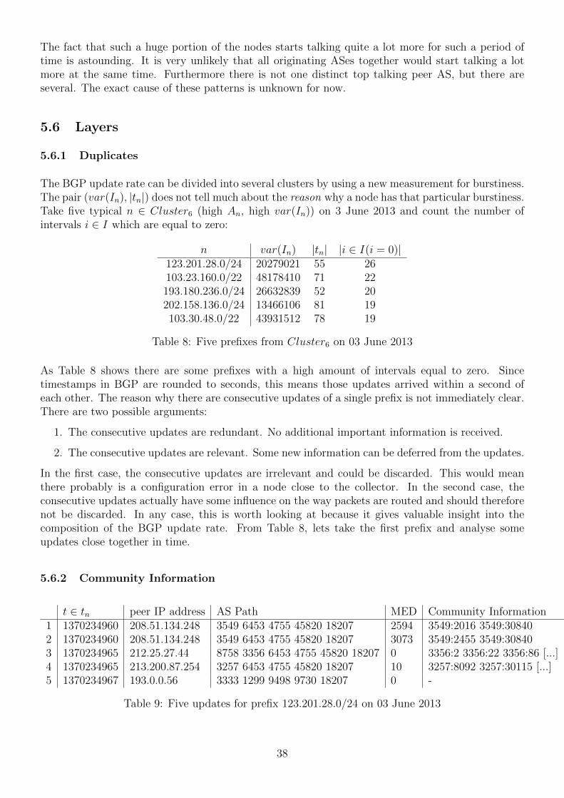
The fact that such a huge portion of the nodes starts talking quite a lot more for such a period oftime is astounding. It is very unlikely that all originating ASes together would start talking a lotmore at the same time. Furthermore there is not one distinct top talking peer AS, but there areseveral. The exact cause of these patterns is unknown for now.

5.6 Layers

5.6.1 Duplicates

The BGP update rate can be divided into several clusters by using a new measurement for burstiness.The pair (var(In), |tn|) does not tell much about the reason why a node has that particular burstiness.Take five typical n ∈ Cluster6 (high An, high var(In)) on 3 June 2013 and count the number ofintervals i ∈ I which are equal to zero:

n var(In) |tn| |i ∈ I(i = 0)|123.201.28.0/24 20279021 55 26103.23.160.0/22 48178410 71 22193.180.236.0/24 26632839 52 20202.158.136.0/24 13466106 81 19103.30.48.0/22 43931512 78 19

Table 8: Five prefixes from Cluster6 on 03 June 2013

As Table 8 shows there are some prefixes with a high amount of intervals equal to zero. Sincetimestamps in BGP are rounded to seconds, this means those updates arrived within a second ofeach other. The reason why there are consecutive updates of a single prefix is not immediately clear.There are two possible arguments:

1. The consecutive updates are redundant. No additional important information is received.

2. The consecutive updates are relevant. Some new information can be deferred from the updates.

In the first case, the consecutive updates are irrelevant and could be discarded. This would meanthere probably is a configuration error in a node close to the collector. In the second case, theconsecutive updates actually have some influence on the way packets are routed and should thereforenot be discarded. In any case, this is worth looking at because it gives valuable insight into thecomposition of the BGP update rate. From Table 8, lets take the first prefix and analyse someupdates close together in time.

5.6.2 Community Information

t ∈ tn peer IP address AS Path MED Community Information1 1370234960 208.51.134.248 3549 6453 4755 45820 18207 2594 3549:2016 3549:308402 1370234960 208.51.134.248 3549 6453 4755 45820 18207 3073 3549:2455 3549:308403 1370234965 212.25.27.44 8758 3356 6453 4755 45820 18207 0 3356:2 3356:22 3356:86 [...]4 1370234965 213.200.87.254 3257 6453 4755 45820 18207 10 3257:8092 3257:30115 [...]5 1370234967 193.0.0.56 3333 1299 9498 9730 18207 0 -

Table 9: Five updates for prefix 123.201.28.0/24 on 03 June 2013

38

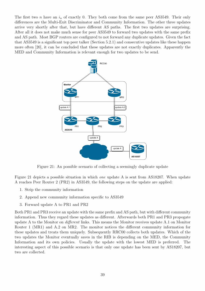
The first two n have an in of exactly 0. They both come from the same peer AS3549. Their onlydifferences are the Multi-Exit Discriminator and Community Information. The other three updatesarrive very shortly after that, but have different AS paths. The first two updates are surprising.After all it does not make much sense for peer AS3549 to forward two updates with the same prefixand AS path. Most BGP routers are configured to not forward any duplicate updates. Given the factthat AS3549 is a significant top peer talker (Section 5.2.1) and consecutive updates like these happenmore often [20], it can be concluded that these updates are not exactly duplicates. Apparently theMED and Community Information is relevant enough for two updates to be send.

Figure 21: An possible scenario of collecting a seemingly duplicate update

Figure 21 depicts a possible situation in which one update A is sent from AS18207. When updateA reaches Peer Router 2 (PR2) in AS3549, the following steps on the update are applied:

1. Strip the community information

2. Append new community information specific to AS3549

3. Forward update A to PR1 and PR2

Both PR1 and PR3 receive an update with the same prefix and AS path, but with different communityinformation. Thus they regard these updates as different. Afterwards both PR1 and PR3 propogateupdate A to the Monitor on different links. This means the Monitor receives update A.1 on MonitorRouter 1 (MR1) and A.2 on MR2. The monitor notices the different community information forthese updates and treats them uniquely. Subsequently RRC00 collects both updates. Which of thetwo updates the Monitor eventually saves in the RIB is depending on the MED, the CommunityInformation and its own policies. Usually the update with the lowest MED is preferred. Theinteresting aspect of this possible scenario is that only one update has been sent by AS18207, buttwo are collected.

39

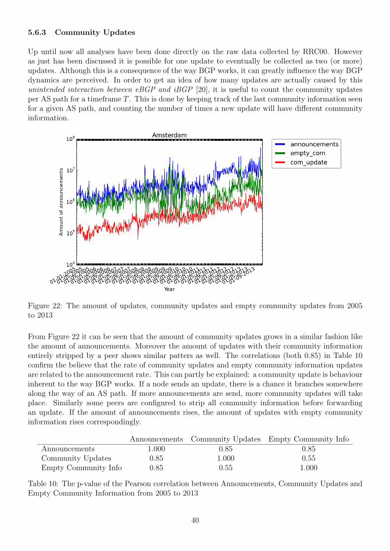
5.6.3 Community Updates

Up until now all analyses have been done directly on the raw data collected by RRC00. Howeveras just has been discussed it is possible for one update to eventually be collected as two (or more)updates. Although this is a consequence of the way BGP works, it can greatly influence the way BGPdynamics are perceived. In order to get an idea of how many updates are actually caused by thisunintended interaction between eBGP and iBGP [20], it is useful to count the community updatesper AS path for a timeframe T . This is done by keeping track of the last community information seenfor a given AS path, and counting the number of times a new update will have different communityinformation.

Figure 22: The amount of updates, community updates and empty community updates from 2005to 2013

From Figure 22 it can be seen that the amount of community updates grows in a similar fashion likethe amount of announcements. Moreover the amount of updates with their community informationentirely stripped by a peer shows similar patters as well. The correlations (both 0.85) in Table 10confirm the believe that the rate of community updates and empty community information updatesare related to the announcement rate. This can partly be explained: a community update is behaviourinherent to the way BGP works. If a node sends an update, there is a chance it branches somewherealong the way of an AS path. If more announcements are send, more community updates will takeplace. Similarly some peers are configured to strip all community information before forwardingan update. If the amount of announcements rises, the amount of updates with empty communityinformation rises correspondingly.

Announcements Community Updates Empty Community InfoAnnouncements 1.000 0.85 0.85Community Updates 0.85 1.000 0.55Empty Community Info 0.85 0.55 1.000

Table 10: The p-value of the Pearson correlation between Announcements, Community Updates andEmpty Community Information from 2005 to 2013

40

5.6.4 Events

Since the Community field provides a way of looking at the dynamics of BGP, it deserves a closerlook. When looking at the update 3 and 4 in Table 9 it can be seen that updates do not necessarilyhave to split at a peer. These two updates arrive at the same time, and have an overlapping righthalf of the AS path. This means they would follow the same path

AS18207→ AS45820→ AS4755→ AS6453

in the beginning. Since both updates arrive at the same time and have a common subroute in the ASpath, it is reasonable to assume that they have branched from one single update. In this case AS6453would be responsible for the branching of the update. Additionally it has been shown in section 5.5.2that BGP updates can be rather bursty. A possible reason for this could be the branching of updatesat certain ASes. By identifying these bursts and grouping their updates together, the underlyingdynamics of originating announcements are revealed.

Let a prefix n ∈ Spref have two states, ON and OFF . By definition a node n has at least oneannouncement. Let such an announcement be caused by an Event En. Any of these conceptual an-nouncements may branch at some point into more announcements before they all reach the collector.Any announcement an arriving at the monitor is registered as an actual new event En if it meets allof the following requirements

1. The node n is in OFF state

2. The AS path in an is different from the currently known AS path for n

3. an is not a community update for the AS path

Once a new En is registered, n is considered to be in the ON state. It stays in the ON state untilthere have not been any incoming an for a specified timeout tout. If no new an have been registeredfor tout seconds, n switches back to OFF . n stays in the ON state if there are an arriving withintervals less than tout. This flow is described in Figure 23.

Figure 23: Event state transition diagram

This model is very similar to the model described by [21]. The difference is in the criteria for a nto switch to ON . In the new model, the announced AS path should not be an community update.As explained in section 5.6.3, a community update for an AS path could just reflect an interactionbetween iBGP and eBGP. Since the purpose of this model is to group relevant an together andcapture an abstraction of originating announcements, a mere community update is not significantenough to be registered as a new event.

41

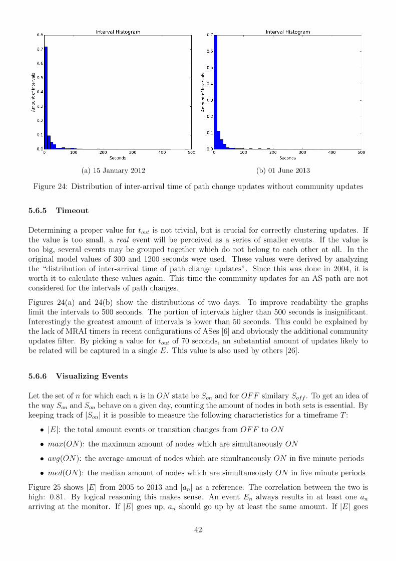
(a) 15 January 2012 (b) 01 June 2013

Figure 24: Distribution of inter-arrival time of path change updates without community updates

5.6.5 Timeout

Determining a proper value for tout is not trivial, but is crucial for correctly clustering updates. Ifthe value is too small, a real event will be perceived as a series of smaller events. If the value istoo big, several events may be grouped together which do not belong to each other at all. In theoriginal model values of 300 and 1200 seconds were used. These values were derived by analyzingthe “distribution of inter-arrival time of path change updates”. Since this was done in 2004, it isworth it to calculate these values again. This time the community updates for an AS path are notconsidered for the intervals of path changes.

Figures 24(a) and 24(b) show the distributions of two days. To improve readability the graphslimit the intervals to 500 seconds. The portion of intervals higher than 500 seconds is insignificant.Interestingly the greatest amount of intervals is lower than 50 seconds. This could be explained bythe lack of MRAI timers in recent configurations of ASes [6] and obviously the additional communityupdates filter. By picking a value for tout of 70 seconds, an substantial amount of updates likely tobe related will be captured in a single E. This value is also used by others [26].

5.6.6 Visualizing Events

Let the set of n for which each n is in ON state be Son and for OFF similary Soff . To get an idea ofthe way Son and Son behave on a given day, counting the amount of nodes in both sets is essential. Bykeeping track of |Son| it is possible to measure the following characteristics for a timeframe T :

• |E|: the total amount events or transition changes from OFF to ON

• max(ON): the maximum amount of nodes which are simultaneously ON

• avg(ON): the average amount of nodes which are simultaneously ON in five minute periods

• med(ON): the median amount of nodes which are simultaneously ON in five minute periods

Figure 25 shows |E| from 2005 to 2013 and |an| as a reference. The correlation between the two ishigh: 0.81. By logical reasoning this makes sense. An event En always results in at least one anarriving at the monitor. If |E| goes up, an should go up by at least the same amount. If |E| goes

42

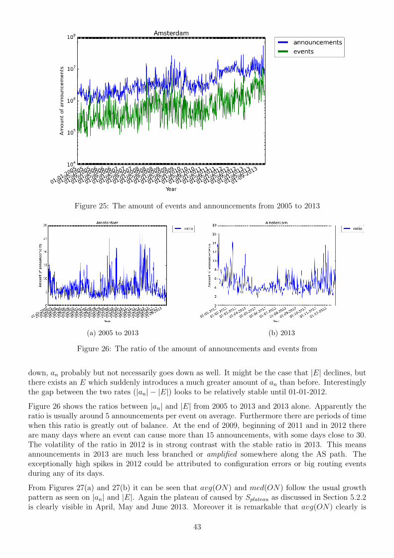
Figure 25: The amount of events and announcements from 2005 to 2013

(a) 2005 to 2013 (b) 2013

Figure 26: The ratio of the amount of announcements and events from

down, an probably but not necessarily goes down as well. It might be the case that |E| declines, butthere exists an E which suddenly introduces a much greater amount of an than before. Interestinglythe gap between the two rates (|an| − |E|) looks to be relatively stable until 01-01-2012.

Figure 26 shows the ratios between |an| and |E| from 2005 to 2013 and 2013 alone. Apparently theratio is usually around 5 announcements per event on average. Furthermore there are periods of timewhen this ratio is greatly out of balance. At the end of 2009, beginning of 2011 and in 2012 thereare many days where an event can cause more than 15 announcements, with some days close to 30.The volatility of the ratio in 2012 is in strong contrast with the stable ratio in 2013. This meansannouncements in 2013 are much less branched or amplified somewhere along the AS path. Theexceptionally high spikes in 2012 could be attributed to configuration errors or big routing eventsduring any of its days.

From Figures 27(a) and 27(b) it can be seen that avg(ON) and med(ON) follow the usual growthpattern as seen on |an| and |E|. Again the plateau of caused by Splateau as discussed in Section 5.2.2is clearly visible in April, May and June 2013. Moreover it is remarkable that avg(ON) clearly is

43

(a) 2005 to 2013 (b) 2013

Figure 27: The average and median amount of nodes simultaneously ON in five minute periods

(a) The amount of Events during 01-01-2007, the mean(green) and median (red)

(b) The ratio of the mean and median from 2005 to2013

Figure 28

much higher at any day than med(ON). This means that the frequency distribution of |E| is skewedto the left. Thus during any day |E| is usually rather low. However there are (multiple) moments atwhich |E| peaks and causes avg(ON) to shift upwards. The fact that avg(ON) does not go belowmed(ON) at any day, is surprising. In essence this implies that there are no deep valleys in the rateof events.

This is shown by Figure 28(a) in more detail. On 01-01-2007 the mean clearly is a lot higher thanthe median. There are five distinct peaks, yet no analogous valleys. In this case the median actuallydepicts a very good measurement for the “center” of the graph. Most of the values are really closeto this line. On the other hand the average is heavily influenced by a few high peaks. FurthermoreFigure 28(b) shows the ratio between mean and median from 2005 to 2013. With the exception ofone day in September 2013, the ratio of the median and mean stays between 100 and 2 × 101. Thefact that this ratio behaves in a fairly constant manner over the years implies that it is not affectedby the growth in amount of updates as seen in Figure 25.

44

6 Aggregated Analysis and Conclusions

Up until now a lot of data, graphs and analyses have been presented. Although some conclusions havealready been formed, the bigger picture is not yet very clear. All the different subsections manifestedin the Results section contribute in a unique way to the essence of this paper. The research questionswere clearly defined in Section 1.2:

• Is it possible to partition the BGP data collected by RRC00 into several distinct layers?

• Why does BGP grow at such a lower rate than the size of the routing table?

• How are irregularities reliably detected?

The first section has shown that BGP is extremely volatile. There are a few distinct peaks causedby session resets. The amount of updates changes so much per day that is it not easy to reveal aconstant pattern. The exact composition of the nodes in the core and list of top talkers varies wildlyas well. So it is not possible to find regular patterns by analyzing individual nodes or prefixes. Onthe other hand the peers did show some regularities. In essence this is all caused by the vastnessof BGP. The sheer amount of nodes, prefixes and possible AS paths makes it very hard to inspectBGP at a detailed level. Efforts to group single nodes of BGP together was to no avail. Thereforeit makes sense to look at BGP behaviour as a whole, and work our way downwards. This top-downapproach proved to be more effective in identifying patterns.

6.1 Top-down

Distributions of updates over nodes and prefixes gives insight in the general dynamics of BGP. Apattern emerges that is seen across most of the distributions. There are a few nodes with a great orlittle impact, and many of them with just lie somewhere in the middle, but very close to each other.The evolution (change in updates over the years) of nodes works in the same fashion.

Additionally it is possible to obtain an approximate measure of the burstiness of a node by calculatingthe variance of its timestamps. Plotting this along with its amount of updates and activeness givesa pattern which is seen throughout the years. The pattern consists of six distinct clusters seen onthe graph. These clusters are easily identifiable by visually analyzing the graphs.

Last but not least by analyzing the amount of events during any day, a baseline pattern is emanate.Although there are heavy fluctuations, there is one aspect clearly recognizable over time. The averageis always higher than the median amount of events. This is caused by short but high peaks of events.Furthermore there are no apparent valleys observed in any of the days, which means there is a specialbaseline of updates. Although there is a chance of a valley occuring at some point, the outright vastamount of nodes makes this change very low.

These three “fingerprints” of BGP are prevalent in all of the observed days.

6.2 Monitoring

In order to detect irregularities in the update rate of BGP, these fingerprints are of great use.Since these fingerprints are commonplace, anything that significantly deviates from them should bebrought to our immediate attention. Throughout this paper two significant irregularities have beenpresented:

• The sudden accelerated boost in |p| and |a| halfway through 2011

45

• The level shift in April, May and June 2013 caused by specific nodes in and near Russia.

Both irregularities have one important distinction: the level shift is transient and characteristic fora subset of nodes, while the accelareted boost is seemingly permanent and widespread. This meanslevel shift is caused by a specific set of nodes and is stopped at some point in time. On the otherhand the increase of the growth factor of |p| and |a| looks to be permanent and originating from abroader cluster, namely pforwhich(19 < ps < 25.

The method used determine the cause of the level shift has some very clear steps which lead to thedesired result. Although it is hard to automate the detection of level shifts, it is possible to manuallymonitor for their existence. Network operators could use this to detect irregularities and high volumelevel shifts on a day to day basis.

• Keep track of the top talking entities (peers, nodes, prefixes) day by day. Any entity with highδ and |a| over a long period of time (plateau) indicates a level shift.

• Analyze the distribution of updates over all nodes. Normally over the time of a month, formleft to right, the graph begins with a very high amount of updates, followed by a steep declineand a gentle curve to a plateau. The graph ends again with a steep decline towards one update.Any prolonged irregularities in this pattern, e.g. additional plateau’s, are indicators of a levelshfit.

• Monitor Cp, Cn and Cpeer the same way. Keep track of enitities with high δ.

• For each node, visualize the burstiness βn and activeness An in one plot. Determine the usualbackground noise and find any suddenly (dis)appearing clusters.

46

7 Summary

The analyses have shown that the BGP update rate is very volatile. There are high peaks occuringthroughout the years. Moreover level-shifts can give a distorted view on the actual baseline updaterate. The sheer volume of updates makes it very difficult to analyse the dynamics of BGP with justsimple scripts. By looking at individual entities in the data there are no clear patterns to be found.The set of originating ASes and prefixes detected in updates changes over time. The “core” of nodesdiminishes over time. Although there is some consistency in the top talking peers, the top talkingoriginating ASes and prefixes show no reliable pattern.

Only by looking at BGP as a whole it becomes apparent that there are some patterns. The updatedistribution shows a smooth curve which is characteristicly present throughout the years. The distri-bution of the growth of the core shows similar characteristics. By measuring the burstiness of nodesit is possible to assess a “fingerprint” of BGP with five distinct clusters. The visual representation ofthese clusters is very constant over the years. By analyzing these plots and spotting anything otherthan these typical BGP characteristics, abnormalties can be found. This can be used to detect levelshifts and possible configuration errors at an early stage.

47

References

[1] Thomas Hallgren, Mark P. Jones, Rebekah Leslie, Andrew Tolmach A Principled Approach toOperating System Construction in Haskell, OGI School of Science & Engineering, Oregon Health& Science University, Department of Computer Science Portand State University

[2] G. Huston, BGP in 2013. APNIC, January 2013.

[3] D. Meyer, L. Zhang, and K. Fall, Report from the IAB workshop on routing and addressinghttp://tools.ietf.org/id/draft-iab-raws-report-02.txt, April 2007.

[4] A. Simula, A. Simula, G. Tech, On the scalability of BGP: the roles of topology growth andupdate rate-limiting Proceedings ACM CoNEXT, December 2008.

[5] G. Huston, The BGP World is Flat!. APNIC, November 2011.

[6] A. Elmokashfi, A. Kvalbein and C. Dovrolis, BGP churn evolution: A perspective from the coreIEEE/ACM Trans. on Networking, vol. 20, no. 2, pp. 571584, April 2012.

[7] Roughan, M., Willinger, W., Maennel, O., Perouli, D., and Bush, 10 lessons from 10 years ofmeasuring and modeling the Internets autonomous systems IEEE Journal on Selected Areas inCommunications 29, 9, 18101821, 2011.

[8] RIS Raw Data, http://www.ripe.net/data-tools/stats/ris/ris-raw-data

[9] TCP/IP Exterior Gateway Protocol (EGP), http://www.tcpipguide.com/free/t TCPIPExteriorGatewayProtocolEGP.htm

[10] E. Rosen, EXTERIOR GATEWAY PROTOCOL (EGP) http://tools.ietf.org/html/rfc827, BoltBeranek and Newman Inc., Octover 1982.

[11] K. Lougheed, Cisco Systems and Y. Rekhter, A Border Gateway Protocol (BGP)http://tools.ietf.org/html/rfc1105 T.J. Watson Research Center, IBM Corp., June 1989.

[12] Y. Rekhter, T. Li and S. Hares, A Border Gateway Protocol 4 (BGP-4)http://www.ietf.org/rfc/rfc4271.txt, January 2006.

[13] J. Hawkinson, BBN Planet and T. Bates, Guidelines for creation, selection, and registration ofan Autonomous System (AS) http://tools.ietf.org/html/rfc1930, March 1996.

[14] R. Chandra, P. Traina, Cisco Systems and T. Li, BGP Communities Attributehttp://tools.ietf.org/html/rfc1997, August 1996.

[15] Y. Rekhter, T. Li, Cisco Systems A Border Gateway Protocol 4 (BGP-4)http://www.ietf.org/rfc/rfc1771.txt T.J. Watson Research Center, IBM Corp., March1995.

[16] Juniper, out-delay http://www.juniper.net/techpubs/en US/junos13.2/topics/reference/configuration-statement/out-delay-edit-protocols-bgp.html

[17] A. Elmokashfi, A. Kvalbein and T. Cicic, On Update Rate-Limiting in BGP IEEE, June 2011.

[18] G. Huston, M. Rossi, and G. Armitage, A Technique for Reducing BGP Update Announcementsthrough Path Exploration Damping Selected Areas in Communications, IEEE Journal on, vol.28, no. 8, pp. 12711286, October 2010.

[19] X. Wang, O. Bonaventure, and P. Zhu, Stabilizing BGP routing without harming convergenceComputer Communications Workshops (INFOCOM WKSHPS), 2011 IEEE Conference on.IEEE April 2011.

48

[20] J. Park, D. Jen, M. Lad, S. Amante, D. McPherson and L. Zhang, Investigating occurrence ofduplicate updates in BGP announcements. Passive and Active Measurement, Springer BerlinHeidelberg, January 2010.

[21] X. Zhao, D. Massey, M. Lad and L. Zhang, On/off model: a new tool to understand bgp updateburst USCCS D, T ech nical Report 4819, 2004.

[22] P. Cheng, X. Zhao, L. Zhang and B. Zhang, Longitudinal study of BGP monitor session failuresACM SIGCOMM Computer Communication Review 40.2: 34-42, 2010.

[23] RIPE Stat, Data API, https://stat.ripe.net/docs/data api

[24] R. Krzanowski, Burst (of packets) and burstiness. 66th IETF meeting, 2006.

[25] S. Deshpande, M. Thottan, T. Ho and B. Sikdar, An online mechanism for BGP instabilitydetection and analysis Computers, IEEE Transactions on 58.11: 1470-1484, 2009.

[26] J. Wu, Z. Mao, J. Rexford and J. Wang, Finding a needle in a haystack: Pinpointing significantBGP routing changes in an IP network Proceedings of the 2nd conference on Symposium onNetworked Systems Design & Implementation-Volume 2. USENIX Association, 2005.

[27] A. Flavel, M. Roughan, N. Bean and O. Maennel, Modeling BGP table fluctuations. ManagingTraffic Performance in Converged Networks. Springer Berlin Heidelberg, 141-153, 2007.

[28] J. Clment, K. Chin, On the characteristics of BGP routes Faculty of Informatics-Papers: 658,2007.

[29] K. Lee, M. Khandani and M. Shayman, Routing Instability in the BGP Protocol Conference onInformation Sciences and Systems, Princeton University, 2004.

49

A Appendix A

A.1 Graph Files

Each daily .graph file includes the following sections made up by many lines, sorted from high tolow amount of updates (N). Do keep in mind that these numbers correspond to the amount of rawupdates received by RRC00. Since this is a multi-hop collector, this will include a lot of duplicateupdates.

peer update|X|N Received N updates from peer AS X

peer announcement|X|N Received N announcements from peer AS X

peer withdrawal|X|N Received N withdrawals from peer AS X

origin announcement|X|N Received N announcement from origin AS X

as path|X|N Received N AS Paths X (top 1000 )

prefix|X|N Received N Prefixes X

as path prefix|X|N Received N AS Paths:Prefix X (top 1000 )

After each section the total amount of N is displayed:

announcements The total amount of announcements

withdrawals The total amount of withdrawals

top 10 prefix announcements The total amount of announcements from the 10 chattiest prefixes

events The total amount of events

max events The maximum amount of concurrent events

min events The minimum amount of concurrent events

median events The median of the amount of concurrent events

mean events The mean of the amount of concurrent events

var events The variance of the amount of concurrent events

std events The standard deviation of the amount of concurrent events

prefixes The total amount of prefixes

empty com The amount of updates with no community information

com update The amount of updates with community information not empty

nag The amount of updates with non aggregated ASes

ag The amount of updates with aggregated ASes

incomplete The amount of incomplete updates

igp The amount of updates caused by an IGP effect

egp The amount of updates caused by an EGP effect

as paths The total amount of distinct AS paths

50

origin ases The amount of distinct originating ASes

suffix For all suffixes [1..64] on a new line, the amount of updates

A.2 Layer Files

Each daily .layers file includes the following sections, along with the total amount of updates

peer update|X|N Received N updates from peer AS X

After each section the total amount of N is displayed:

total [section]|N Received N in total

B Appendix B

B.0.1 graph.py

This script takes a city name, start year, end year and graph type (origin announcement, prefix,as path or as path prefix). It loops recursively over all .graph files found in the directory city andreads them line by line. If the current line equals the specified graph type, it stores the amount (N)for each type (X) in a dictionary. In the case of prefixes, it also keeps track of the amount of ipv4and ipv6 prefixes. A user specified subset of X is plotted using time (years) on the x-axis versusamount (N) of graph type on the y-axis. This way the growth or decline trends of BGP updates canbe analysed.

B.0.2 growth.py

This script takes a type X and two seperate directories with .graph files and compares the content.The start set is defined as a list of AS numbers, prefixes or AS paths which are present in the firstdirectory. The end set works the same way. The core set is the intersection of the start and end set.The growth of the start, end and core set is measured and its distribution plotted. This way theconsistency of the content of BGP updates can be measured.

B.0.3 hist.py

This script takes a type X and directory. Again it reads all .graph files and filters and sorts thecontent on type and amount. Then it plots the distribution of the amount of days all X are active, orthe distribution of the amount of updates all X have sent. This way an insight in averages, mediansand quantiles over the speicified set is gained.

B.0.4 top.py

This script takes a directory containing the .graph files. It sorts all the data on amount or activedays and outputs the top 10 of all types.

51