Beyond the Kalman FilterParticle Filters for Tracking Applications
47
• Beyond the Kalman Filter: Particle filters for tracking applications N. J. Gordon Tracking and Sensor Fusion Group Intelligence, Surveillance and Reconnaissance Division Defence Science and Technology Organisation PO Box 1500, Edinburgh, SA 5111, AUSTRALIA. [email protected] N.J. Gordon : Lake Louise : October 2003 – p. 1/47
description
kalman, particle filter
Transcript of Beyond the Kalman FilterParticle Filters for Tracking Applications

•
Beyond the Kalman Filter:
Particle filters for tracking applications
N. J. Gordon
Tracking and Sensor Fusion Group
Intelligence, Surveillance and Reconnaissance Division
Defence Science and Technology Organisation
PO Box 1500, Edinburgh, SA 5111, AUSTRALIA.
N.J. Gordon : Lake Louise : October 2003 – p. 1/47
•
Contents
– General PF discussion
– History
– Review
– Tracking applications
– Sonobuoy
– TBD
– DBZ
N.J. Gordon : Lake Louise : October 2003 – p. 2/47
•
What is tracking?
– Use models of the real world to
– estimate the past and present
– predict the future
– Achieved by extracting underlying information from
sequence of noisy/uncertain observations
– Perform inference on-line
– Evaluate evolving sequence of probability distributions
N.J. Gordon : Lake Louise : October 2003 – p. 3/47
•
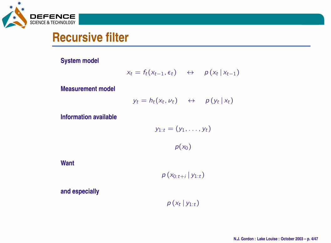
Recursive filter
System model
xt = ft(xt`1; ›t) $ p (xt xt`1)
Measurement model
yt = ht(xt ; �t) $ p (yt xt)
Information available
y1:t = (y1; : : : ; yt)
p(x0)
Want
p (x0:t+i y1:t)
and especially
p (xt y1:t)
N.J. Gordon : Lake Louise : October 2003 – p. 4/47
•
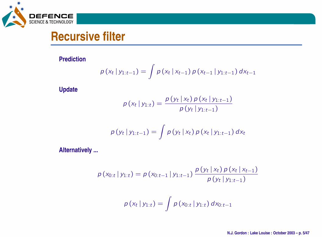
Recursive filter
Prediction
p (xt y1:t`1) =∫
p (xt xt`1) p (xt`1 y1:t`1) dxt`1
Update
p (xt y1:t) =p (yt xt) p (xt y1:t`1)
p (yt y1:t`1)
p (yt y1:t`1) =∫
p (yt xt) p (xt y1:t`1) dxt
Alternatively ...
p (x0:t y1:t) = p (x0:t`1 y1:t`1)p (yt xt) p (xt xt`1)
p (yt y1:t`1)
p (xt y1:t) =
∫
p (x0:t y1:t) dx0:t`1
N.J. Gordon : Lake Louise : October 2003 – p. 5/47
•
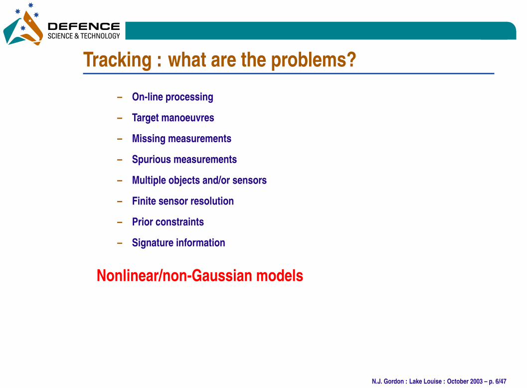
Tracking : what are the problems?
– On-line processing
– Target manoeuvres
– Missing measurements
– Spurious measurements
– Multiple objects and/or sensors
– Finite sensor resolution
– Prior constraints
– Signature information
Nonlinear/non-Gaussian models
N.J. Gordon : Lake Louise : October 2003 – p. 6/47
•
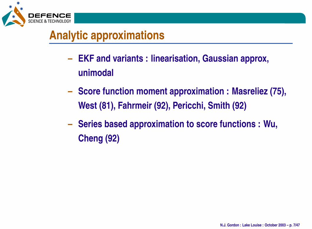
Analytic approximations
– EKF and variants : linearisation, Gaussian approx,
unimodal
– Score function moment approximation : Masreliez (75),
West (81), Fahrmeir (92), Pericchi, Smith (92)
– Series based approximation to score functions : Wu,
Cheng (92)
N.J. Gordon : Lake Louise : October 2003 – p. 7/47
•
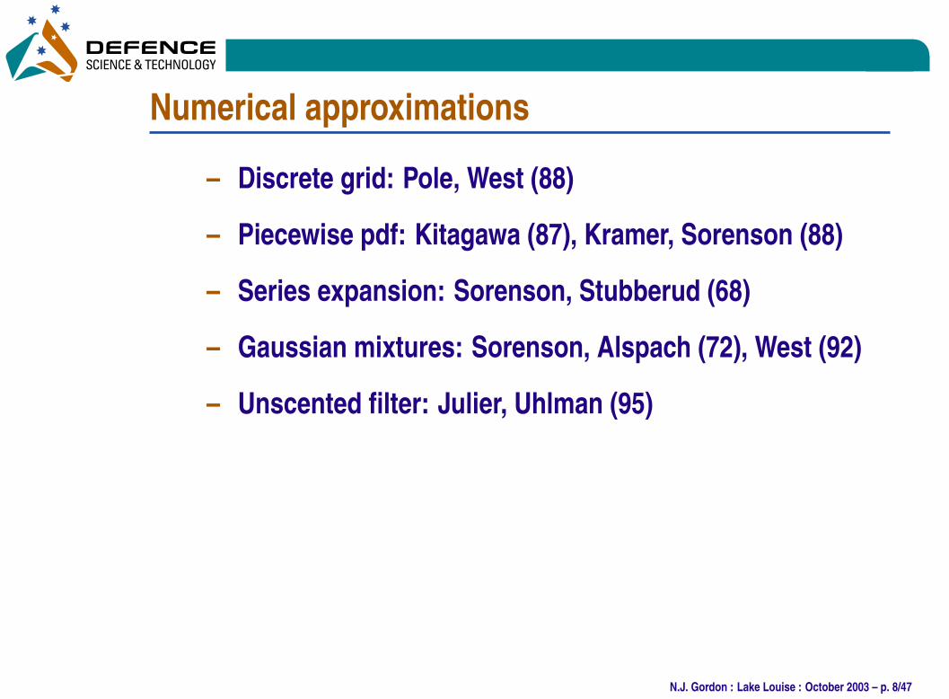
Numerical approximations
– Discrete grid: Pole, West (88)
– Piecewise pdf: Kitagawa (87), Kramer, Sorenson (88)
– Series expansion: Sorenson, Stubberud (68)
– Gaussian mixtures: Sorenson, Alspach (72), West (92)
– Unscented filter: Julier, Uhlman (95)
N.J. Gordon : Lake Louise : October 2003 – p. 8/47
•
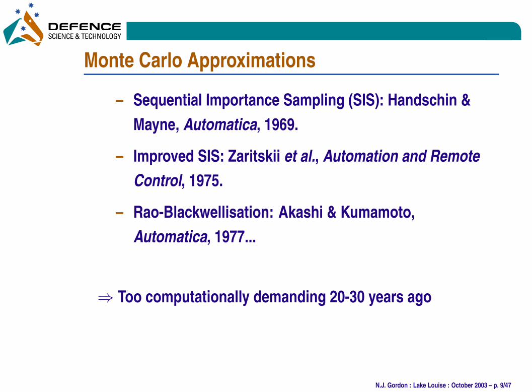
Monte Carlo Approximations
– Sequential Importance Sampling (SIS): Handschin &
Mayne, Automatica, 1969.
– Improved SIS: Zaritskii et al., Automation and Remote
Control, 1975.
– Rao-Blackwellisation: Akashi & Kumamoto,
Automatica, 1977...
) Too computationally demanding 20-30 years ago
N.J. Gordon : Lake Louise : October 2003 – p. 9/47

•
Sequential Monte Carlo (SMC)
– SMC methods lead to estimate of the completeprobability distribution
– Approximation centred on the pdf rather thancompromising the state space model
– Known as Particle filters, SIR filters, bootstrapfilters, Monte Carlo filters, Condensation etc
N.J. Gordon : Lake Louise : October 2003 – p. 10/47
•
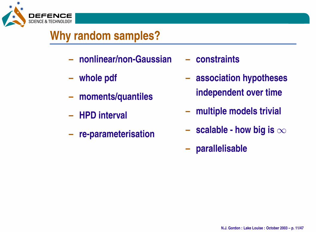
Why random samples?
– nonlinear/non-Gaussian
– whole pdf
– moments/quantiles
– HPD interval
– re-parameterisation
– constraints
– association hypotheses
independent over time
– multiple models trivial
– scalable - how big is1
– parallelisable
N.J. Gordon : Lake Louise : October 2003 – p. 11/47
•
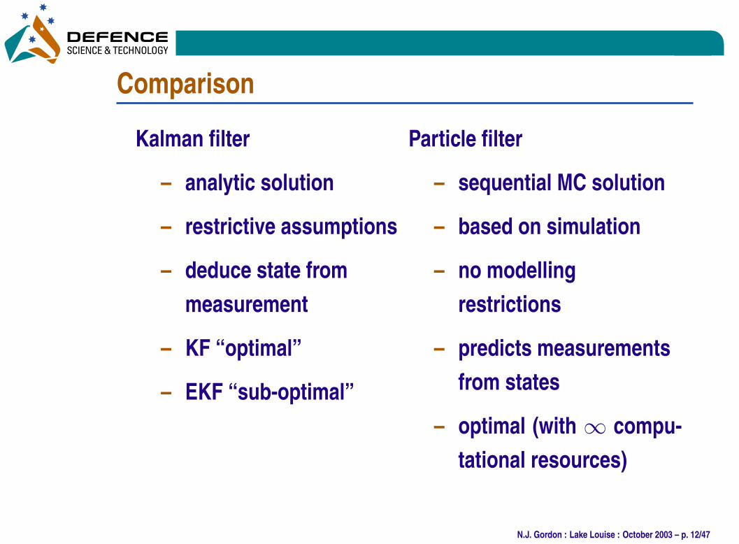
Comparison
Kalman filter
– analytic solution
– restrictive assumptions
– deduce state from
measurement
– KF “optimal”
– EKF “sub-optimal”
Particle filter
– sequential MC solution
– based on simulation
– no modelling
restrictions
– predicts measurements
from states
– optimal (with 1 compu-
tational resources)
N.J. Gordon : Lake Louise : October 2003 – p. 12/47

•Book Advert
Sequential Monte Carlo methods in practice
Editors: Doucet, de Freitas, Gordon
Springer-Verlag (2001)
– Theoretical Foundations
– Efficiency Measures
– Applications :
– Target tracking, missile guidance, image tracking, terrain referenced
navigation, exchange rate prediction, portfolio allocation, in-situ
ellipsometry, pollution monitoring, communications and audio engineering.
N.J. Gordon : Lake Louise : October 2003 – p. 13/47
•
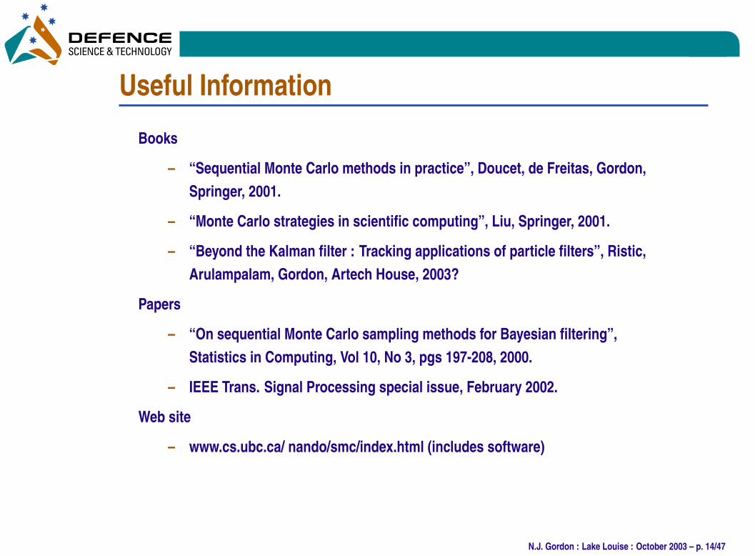
Useful Information
Books
– “Sequential Monte Carlo methods in practice”, Doucet, de Freitas, Gordon,
Springer, 2001.
– “Monte Carlo strategies in scientific computing”, Liu, Springer, 2001.
– “Beyond the Kalman filter : Tracking applications of particle filters”, Ristic,
Arulampalam, Gordon, Artech House, 2003?
Papers
– “On sequential Monte Carlo sampling methods for Bayesian filtering”,
Statistics in Computing, Vol 10, No 3, pgs 197-208, 2000.
– IEEE Trans. Signal Processing special issue, February 2002.
Web site
– www.cs.ubc.ca/ nando/smc/index.html (includes software)
N.J. Gordon : Lake Louise : October 2003 – p. 14/47
•
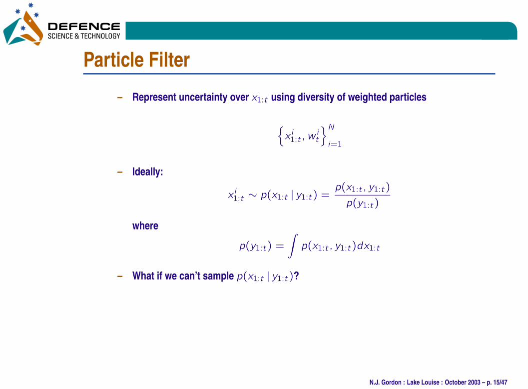
Particle Filter
– Represent uncertainty over x1:t using diversity of weighted particles
{
x i1:t ; wit
}N
i=1
– Ideally:
x i1:t ‰ p(x1:t j y1:t) =p(x1:t ; y1:t)
p(y1:t)
where
p(y1:t) =
∫
p(x1:t ; y1:t)dx1:t
– What if we can’t sample p(x1:t j y1:t)?
N.J. Gordon : Lake Louise : October 2003 – p. 15/47
•
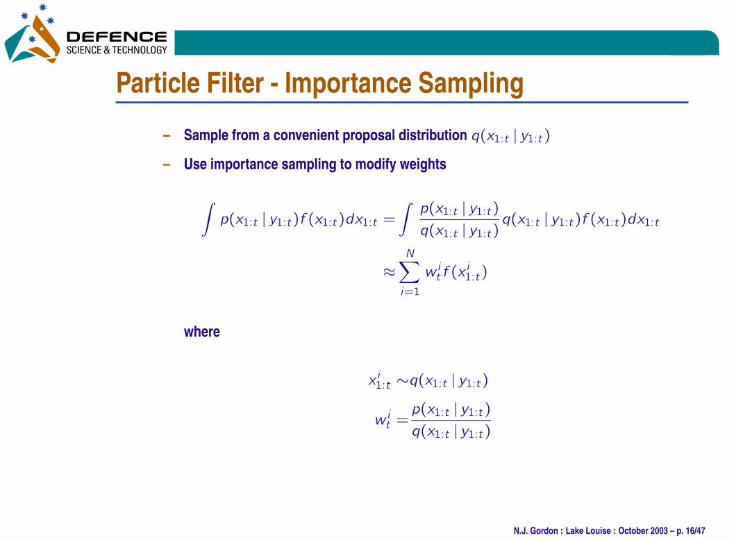
Particle Filter - Importance Sampling
– Sample from a convenient proposal distribution q(x1:t j y1:t)
– Use importance sampling to modify weights
∫
p(x1:t j y1:t)f (x1:t)dx1:t =∫p(x1:t j y1:t)q(x1:t j y1:t)
q(x1:t j y1:t)f (x1:t)dx1:t
ıN∑
i=1
w it f (xi1:t)
where
x i1:t ‰q(x1:t j y1:t)
w it =p(x1:t j y1:t)q(x1:t j y1:t)
N.J. Gordon : Lake Louise : October 2003 – p. 16/47
•
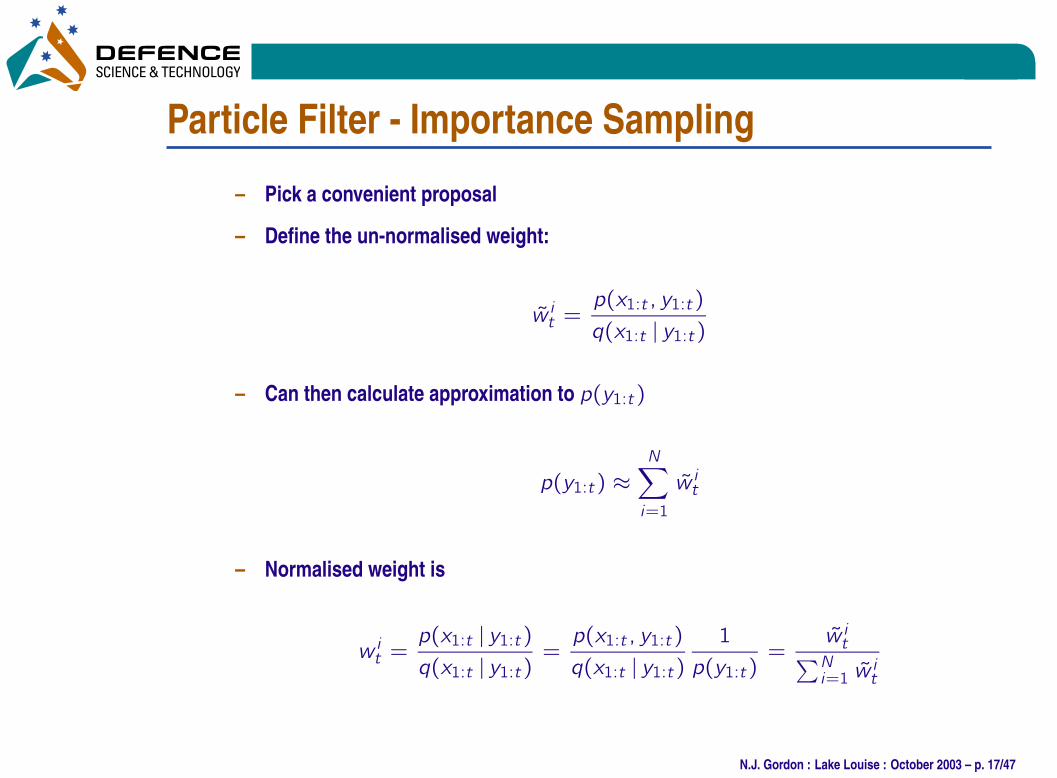
Particle Filter - Importance Sampling
– Pick a convenient proposal
– Define the un-normalised weight:
~w it =p(x1:t ; y1:t)
q(x1:t j y1:t)
– Can then calculate approximation to p(y1:t)
p(y1:t) ıN∑
i=1
~w it
– Normalised weight is
w it =p(x1:t j y1:t)q(x1:t j y1:t)
=p(x1:t ; y1:t)
q(x1:t j y1:t)1
p(y1:t)=
~w it∑Ni=1 ~w
it
N.J. Gordon : Lake Louise : October 2003 – p. 17/47
•
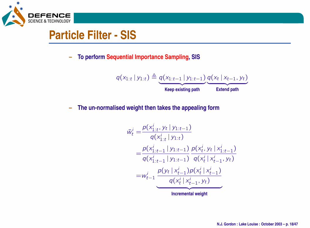
Particle Filter - SIS
– To perform Sequential Importance Sampling, SIS
q(x1:t j y1:t) , q(x1:t`1 j y1:t`1)︸ ︷︷ ︸
Keep existing path
q(xt j xt`1; yt)︸ ︷︷ ︸
Extend path
– The un-normalised weight then takes the appealing form
~w it =p(x i1:t ; yt j y1:t`1)q(x i1:t j y1:t)
=p(x i1:t`1 j y1:t`1)q(x i1:t`1 j y1:t`1)
p(x it ; yt j x i1:t`1)q(x it j x it`1; yt)
=w it`1p(yt j x it`1)p(x it j x it`1)q(x it j x it`1; yt)
︸ ︷︷ ︸
Incremental weight
N.J. Gordon : Lake Louise : October 2003 – p. 18/47
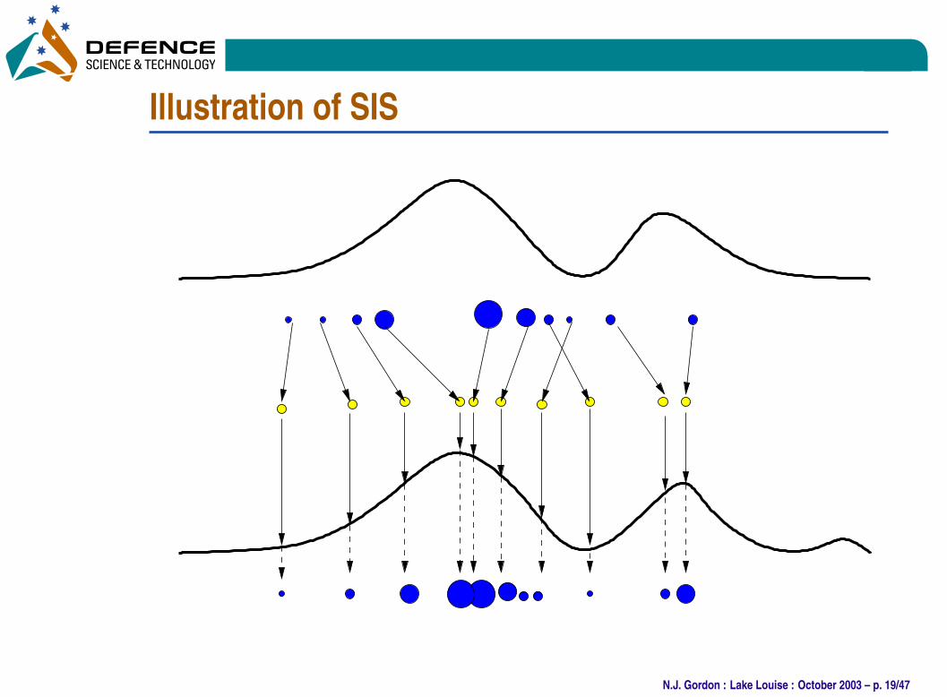
•
Illustration of SIS
N.J. Gordon : Lake Louise : October 2003 – p. 19/47
•
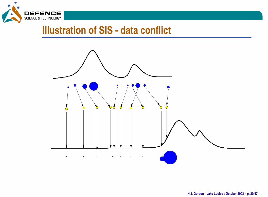
Illustration of SIS - data conflict
N.J. Gordon : Lake Louise : October 2003 – p. 20/47
•
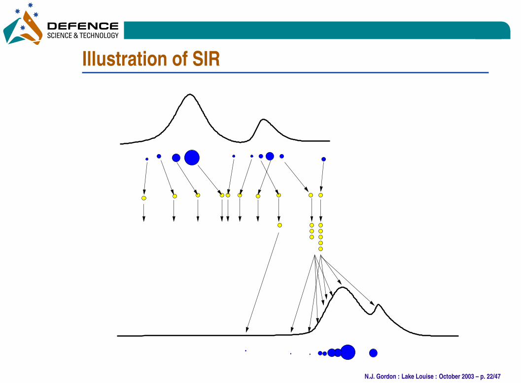
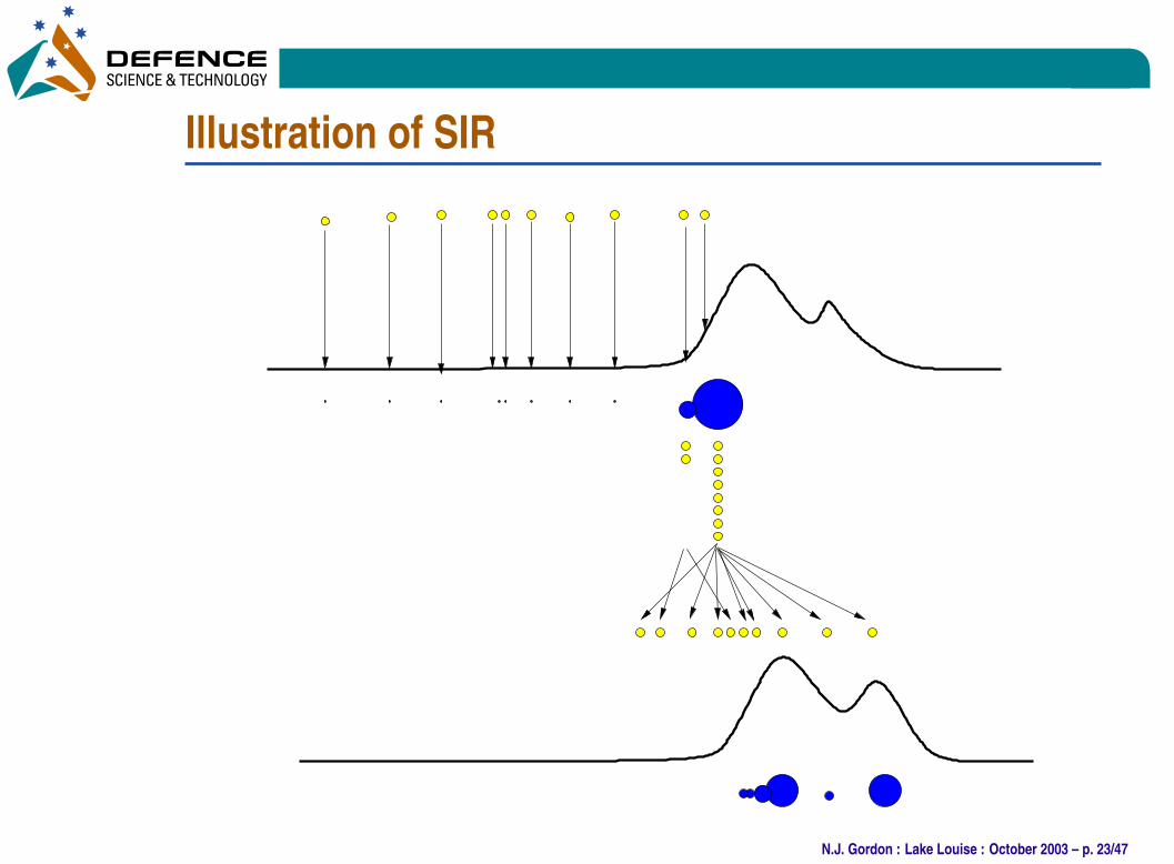
SIS
Problem : Whatever the importance function, degeneracy is observed (Kong, Liu and Wong
1994).
– Introduce a selection scheme to discard/multiply particles x i0:t with respectively
high/low importance weights
– Resampling maps the weighted random measure (x i0:t ; wt) onto the equally
weighted random measure (x i0:t ; N`1)
– Scheme generatesNi children such that∑Ni=1 Ni = N and satisfies
E(Ni ) = Nwik
N.J. Gordon : Lake Louise : October 2003 – p. 21/47
•
Illustration of SIR
N.J. Gordon : Lake Louise : October 2003 – p. 22/47
•
Illustration of SIR
N.J. Gordon : Lake Louise : October 2003 – p. 23/47
•
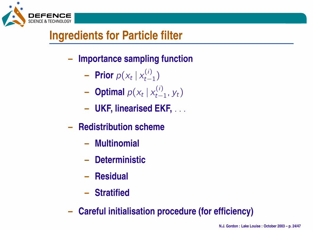
Ingredients for Particle filter
– Importance sampling function
– Prior p(xt j x(i)t`1)
– Optimal p(xt j x(i)t`1; yt)
– UKF, linearised EKF, : : :
– Redistribution scheme
– Multinomial
– Deterministic
– Residual
– Stratified
– Careful initialisation procedure (for efficiency)
N.J. Gordon : Lake Louise : October 2003 – p. 24/47
•
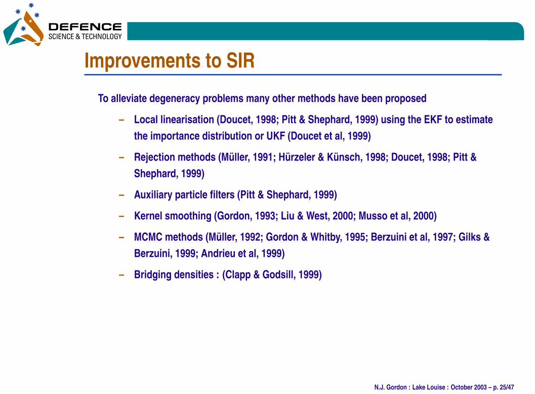
Improvements to SIR
To alleviate degeneracy problems many other methods have been proposed
– Local linearisation (Doucet, 1998; Pitt & Shephard, 1999) using the EKF to estimate
the importance distribution or UKF (Doucet et al, 1999)
– Rejection methods (Müller, 1991; Hürzeler & Künsch, 1998; Doucet, 1998; Pitt &
Shephard, 1999)
– Auxiliary particle filters (Pitt & Shephard, 1999)
– Kernel smoothing (Gordon, 1993; Liu & West, 2000; Musso et al, 2000)
– MCMC methods (Müller, 1992; Gordon & Whitby, 1995; Berzuini et al, 1997; Gilks &
Berzuini, 1999; Andrieu et al, 1999)
– Bridging densities : (Clapp & Godsill, 1999)
N.J. Gordon : Lake Louise : October 2003 – p. 25/47
•
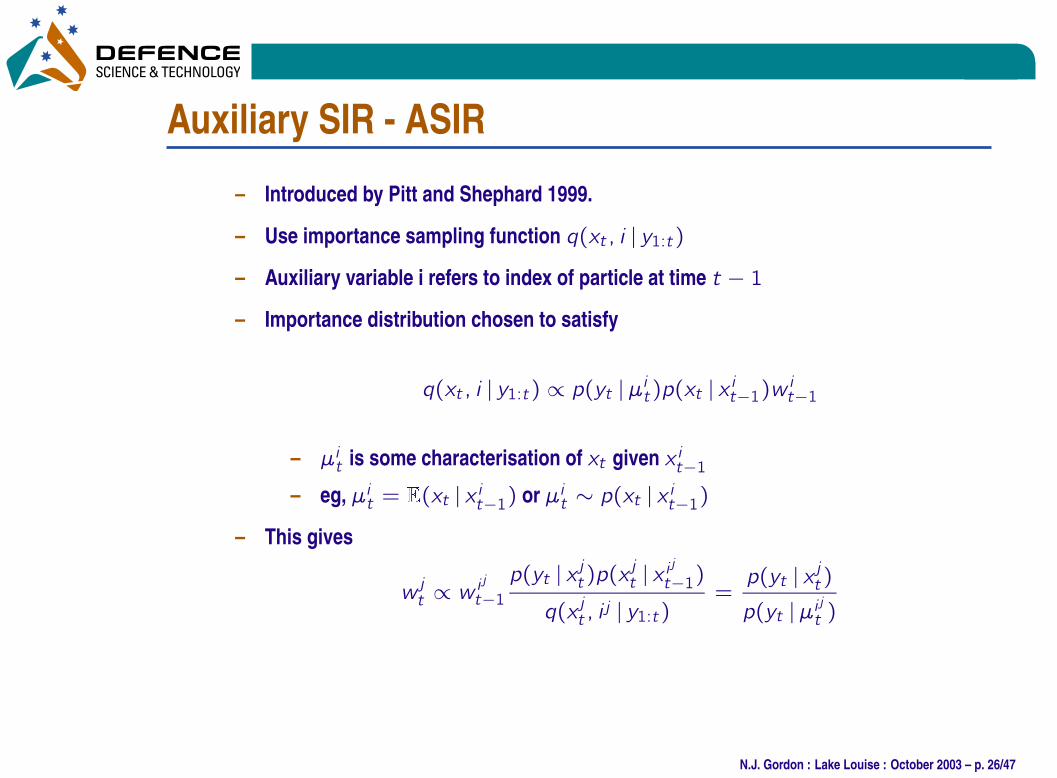
Auxiliary SIR - ASIR
– Introduced by Pitt and Shephard 1999.
– Use importance sampling function q(xt ; i j y1:t)
– Auxiliary variable i refers to index of particle at time t ` 1
– Importance distribution chosen to satisfy
q(xt ; i j y1:t) / p(yt j—it)p(xt j x it`1)w it`1
– —it is some characterisation of xt given x it`1– eg, —it = E(xt j x it`1) or —it ‰ p(xt j x it`1)
– This gives
w jt / w ij
t`1p(yt j x jt )p(x
jt j x i
j
t`1)
q(x jt ; ij j y1:t)
=p(yt j x jt )p(yt j—i jt )
N.J. Gordon : Lake Louise : October 2003 – p. 26/47
•
ASIR
– Naturally uses points at t ` 1 which are “close” to
measurement yt
– If process noise is small then ASIR less sensitive to
outliers than SIR
– This is because single point —it characterises
p(xt j xt`1) well
– But if process noise is large then ASIR can degrade
performance
– Since a single point —it does not characterise
p(xt j xt`1)
N.J. Gordon : Lake Louise : October 2003 – p. 27/47
•
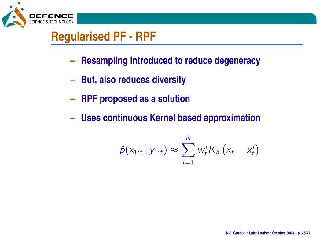
Regularised PF - RPF
– Resampling introduced to reduce degeneracy
– But, also reduces diversity
– RPF proposed as a solution
– Uses continuous Kernel based approximation
p̂(x1:t j y1:t) ı
N∑
i=1
w itKh(xt ` x
it
)
N.J. Gordon : Lake Louise : October 2003 – p. 28/47
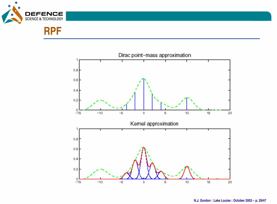
•RPF
N.J. Gordon : Lake Louise : October 2003 – p. 29/47
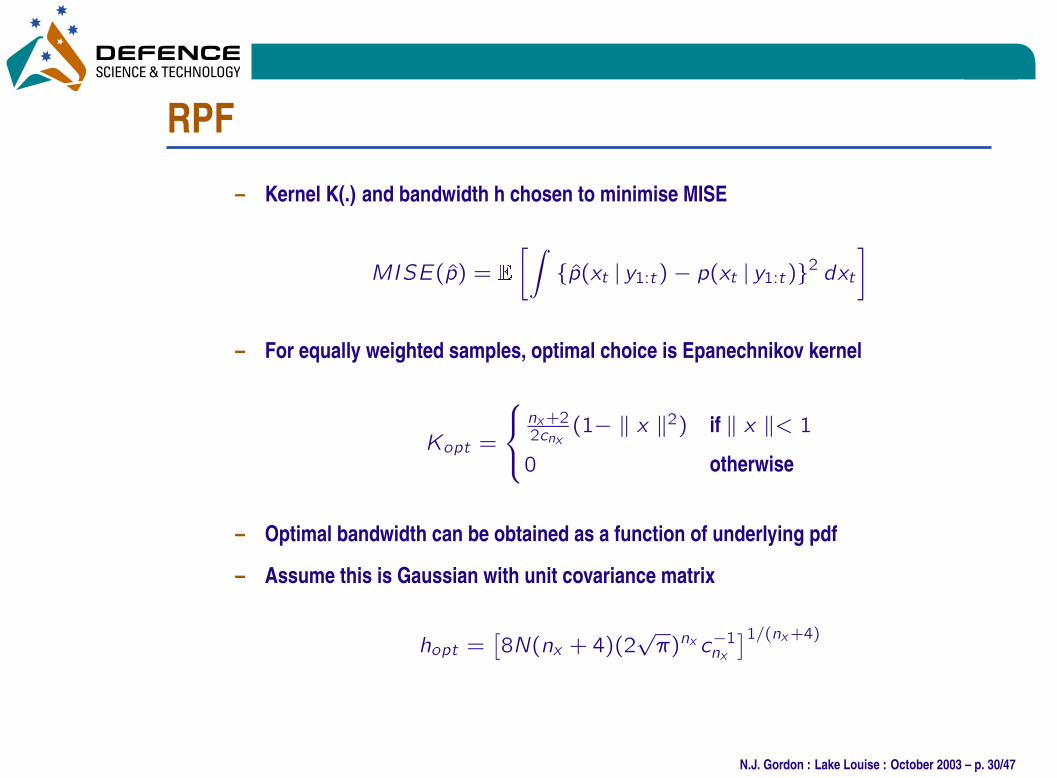
•RPF
– Kernel K(.) and bandwidth h chosen to minimise MISE
MISE(p̂) = E[∫ fp̂(xt j y1:t)` p(xt j y1:t)g2 dxt]– For equally weighted samples, optimal choice is Epanechnikov kernel
Kopt =
nx+22cnx(1` k x k2) if k x k< 1
0 otherwise
– Optimal bandwidth can be obtained as a function of underlying pdf
– Assume this is Gaussian with unit covariance matrix
hopt =[8N(nx + 4)(2
pı)nx c`1nx
]1=(nx+4)
N.J. Gordon : Lake Louise : October 2003 – p. 30/47
•
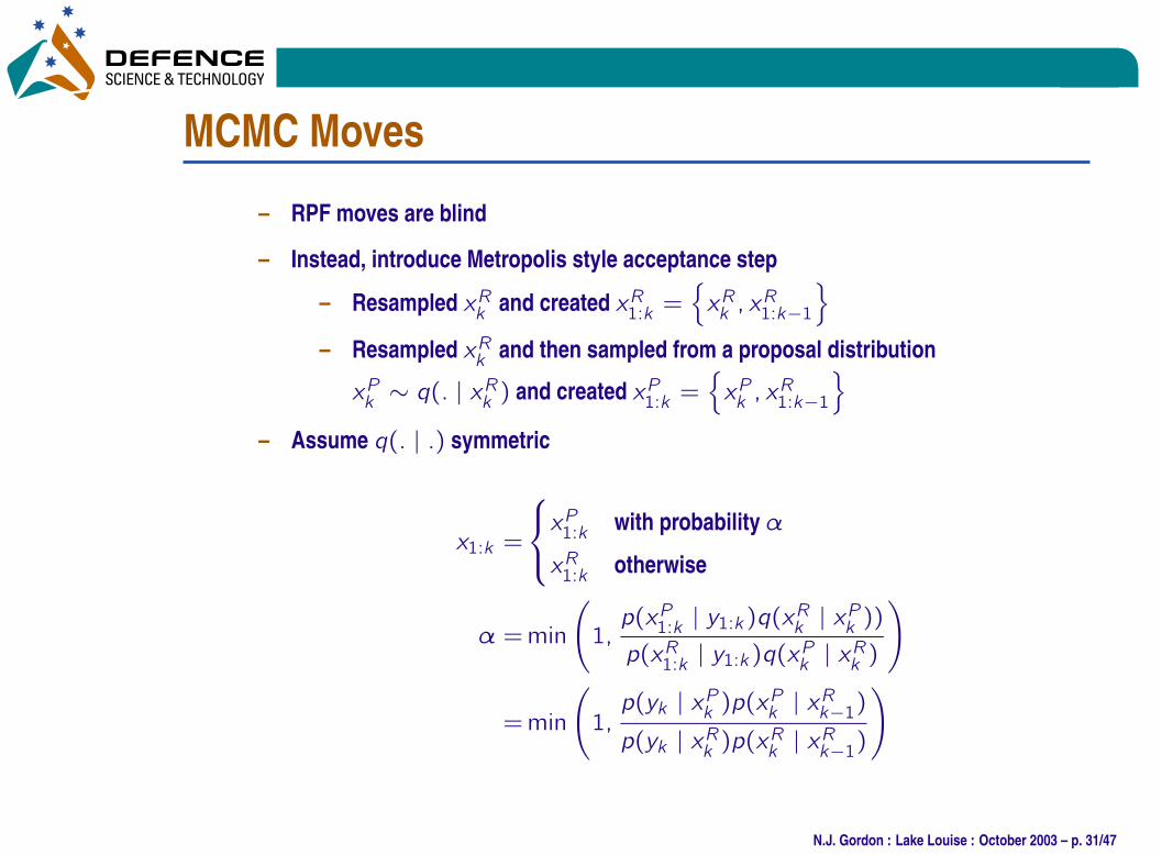
MCMC Moves
– RPF moves are blind
– Instead, introduce Metropolis style acceptance step
– Resampled xRk and created xR1:k ={
xRk ; xR1:k`1
}
– Resampled xRk and then sampled from a proposal distribution
xPk ‰ q(: j xRk ) and created xP1:k ={
xPk ; xR1:k`1
}
– Assume q(: j :) symmetric
x1:k =
xP1:k with probability ¸
xR1:k otherwise
¸ =min
(
1;p(xP1:k j y1:k)q(xRk j xPk ))p(xR1:k j y1:k)q(xPk j xRk )
)
=min
(
1;p(yk j xPk )p(xPk j xRk`1)p(yk j xRk )p(xRk j xRk`1)
)
N.J. Gordon : Lake Louise : October 2003 – p. 31/47
•
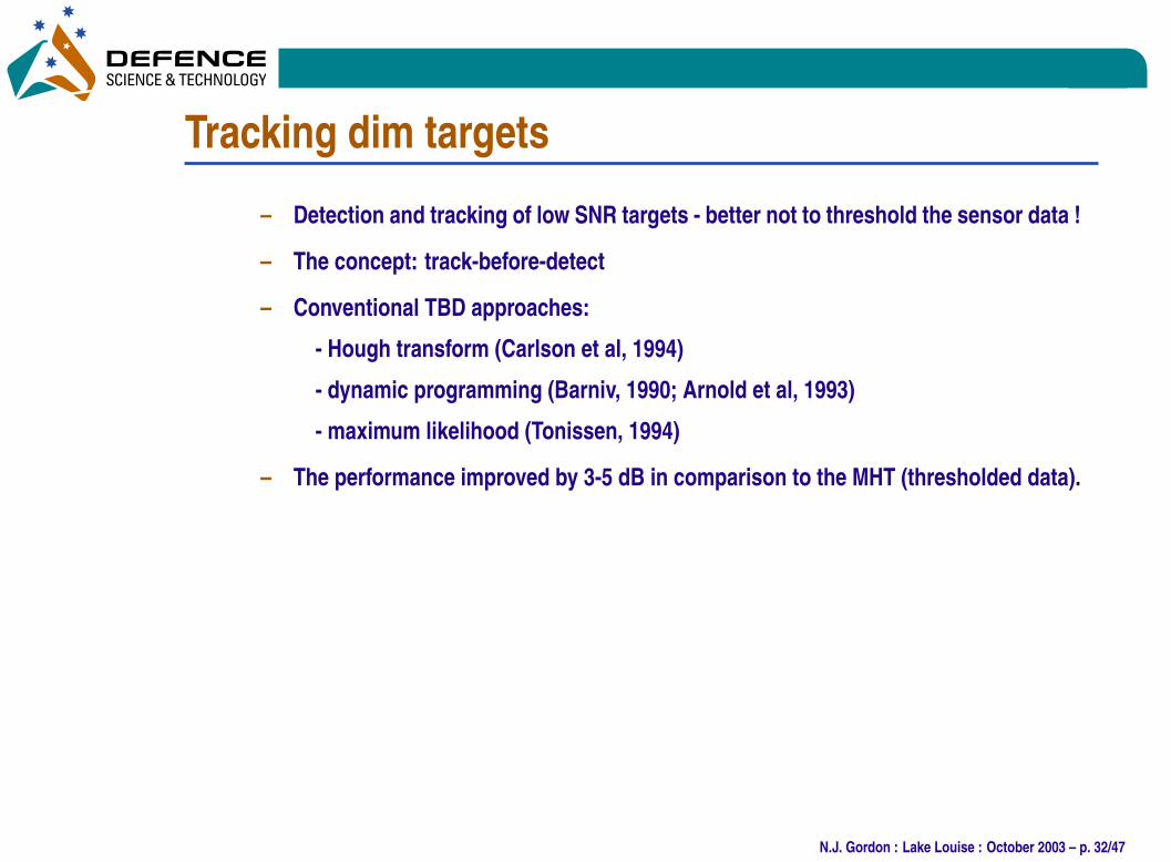
Tracking dim targets
– Detection and tracking of low SNR targets - better not to threshold the sensor data !
– The concept: track-before-detect
– Conventional TBD approaches:
- Hough transform (Carlson et al, 1994)
- dynamic programming (Barniv, 1990; Arnold et al, 1993)
- maximum likelihood (Tonissen, 1994)
– The performance improved by 3-5 dB in comparison to the MHT (thresholded data).
N.J. Gordon : Lake Louise : October 2003 – p. 32/47
•
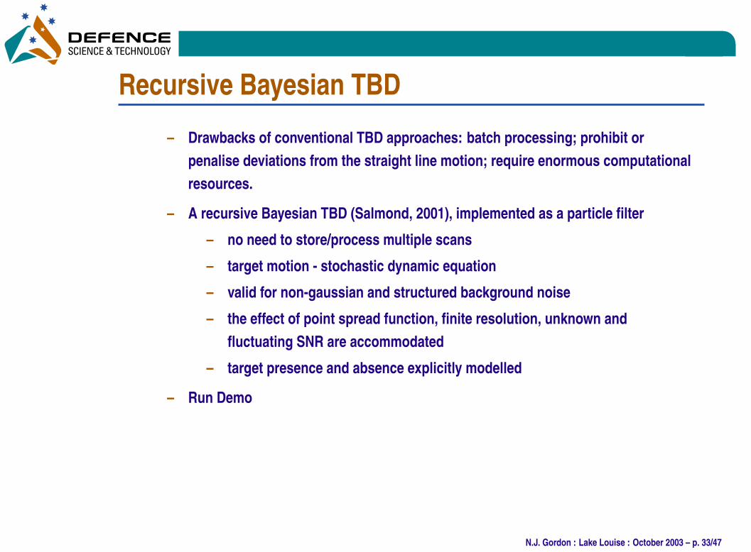
Recursive Bayesian TBD
– Drawbacks of conventional TBD approaches: batch processing; prohibit or
penalise deviations from the straight line motion; require enormous computational
resources.
– A recursive Bayesian TBD (Salmond, 2001), implemented as a particle filter
– no need to store/process multiple scans
– target motion - stochastic dynamic equation
– valid for non-gaussian and structured background noise
– the effect of point spread function, finite resolution, unknown and
fluctuating SNR are accommodated
– target presence and absence explicitly modelled
– Run Demo
N.J. Gordon : Lake Louise : October 2003 – p. 33/47
•
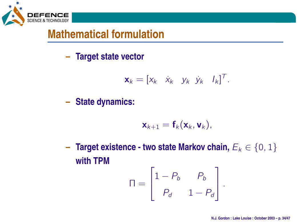
Mathematical formulation
– Target state vector
xk = [xk _xk yk _yk Ik ]T :
– State dynamics:
xk+1 = fk(xk ; vk);
– Target existence - two state Markov chain, Ek 2 f0; 1g
with TPM
˝ =
1` Pb Pb
Pd 1` Pd
:
N.J. Gordon : Lake Louise : October 2003 – p. 34/47
•
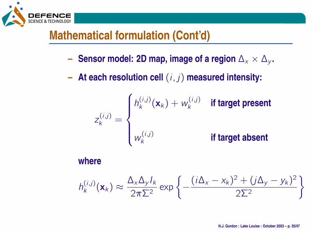
Mathematical formulation (Cont’d)
– Sensor model: 2D map, image of a region ´x ˆ ´y .
– At each resolution cell (i ; j) measured intensity:
z(i ;j)k =
h(i ;j)k (xk) + w
(i ;j)k if target present
w(i ;j)k if target absent
where
h(i ;j)k (xk) ı
´x´y Ik2ı˚2
exp
{
`(i´x ` xk)
2 + (j´y ` yk)2
2˚2
}
N.J. Gordon : Lake Louise : October 2003 – p. 35/47
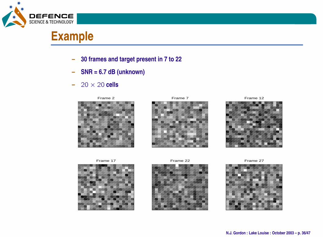
•Example
– 30 frames and target present in 7 to 22
– SNR = 6.7 dB (unknown)
– 20ˆ 20 cells
Frame 2
Frame 7
Frame 12
Frame 17
Frame 22
Frame 27
N.J. Gordon : Lake Louise : October 2003 – p. 36/47
•
Particle filter output (6 states)
Figures suppressed to reduce file size.
N.J. Gordon : Lake Louise : October 2003 – p. 37/47
•
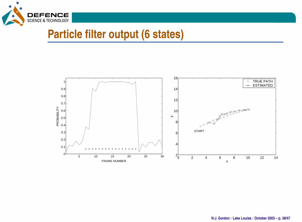
Particle filter output (6 states)
5 10 15 20 25 300
0.1
0.2
0.3
0.4
0.5
0.6
0.7
0.8
0.9
1
FRAME NUMBER
PR
OB
AB
ILIT
Y
0 2 4 6 8 10 12 142
4
6
8
10
12
14
16
x
y
TRUE PATHESTIMATED
START
N.J. Gordon : Lake Louise : October 2003 – p. 38/47
•
PF based TBD - Performance
– Derived CRLBs (as a function of SNR)
– Compared PF-TBD to CRLBs
– Detection and Tracking reliable at 5 dB (or higher)
N.J. Gordon : Lake Louise : October 2003 – p. 39/47
•
Sonobuoy and Submarine
– Noisy bearing measurements from drifting sensors
– Uncertainty in sensor locations
– Sensor loss
– High proportion of spurious bearing measurements
– Run demo
N.J. Gordon : Lake Louise : October 2003 – p. 40/47
•
Blind Doppler
– Blind Doppler zone to to filter out ground clutter +
ground moving targets
– A simple EP measure against any CW or pulse Doppler
radar
– Causes track loss
– Aided by on-board RWR or ESM
N.J. Gordon : Lake Louise : October 2003 – p. 41/47
•
Tracking with hard constraints
– Prior information on sensor constraints
– Posterior pdf is truncated (non-Gaussian)
– Example :
– 2-D tracking with CV model
– (r; „; _r) measurements
– pd < 1
– EKF and Particle Filter with identical gating and
track scoring
N.J. Gordon : Lake Louise : October 2003 – p. 42/47
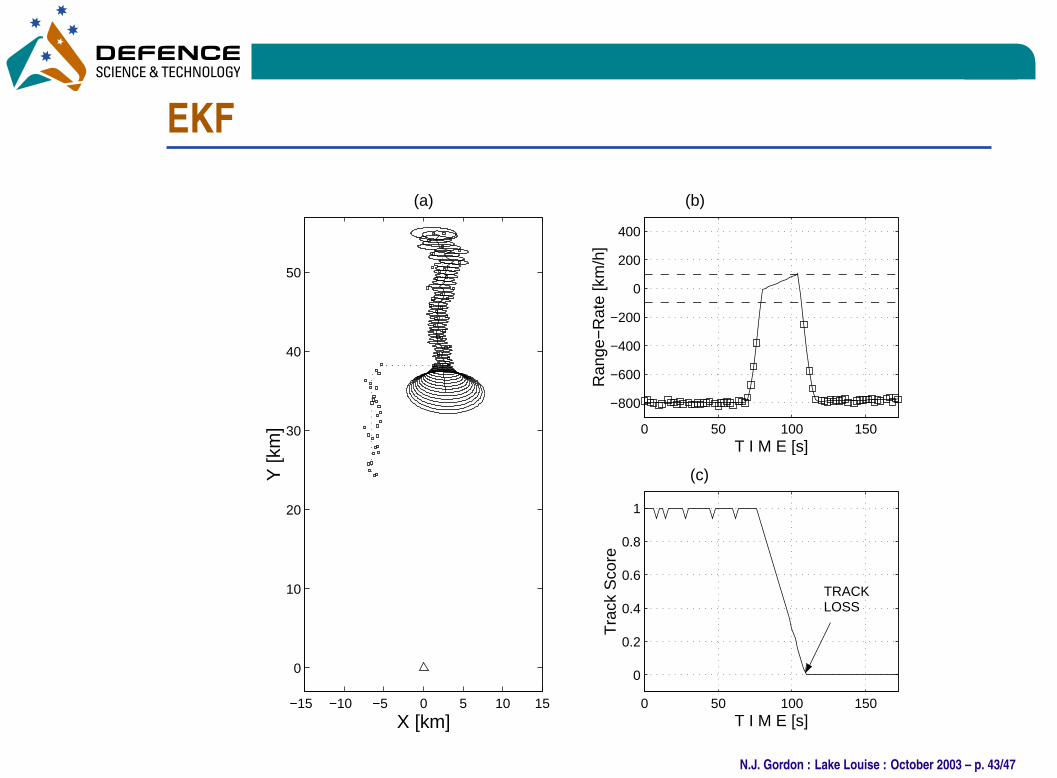
•EKF
−15 −10 −5 0 5 10 15
0
10
20
30
40
50
X [km]
Y [k
m]
(a)
0 50 100 150
0
0.2
0.4
0.6
0.8
1
T I M E [s]
Tra
ck S
core
(c)
0 50 100 150
−800
−600
−400
−200
0
200
400
T I M E [s]
Ran
ge−
Rat
e [k
m/h
]
(b)
TRACKLOSS
N.J. Gordon : Lake Louise : October 2003 – p. 43/47
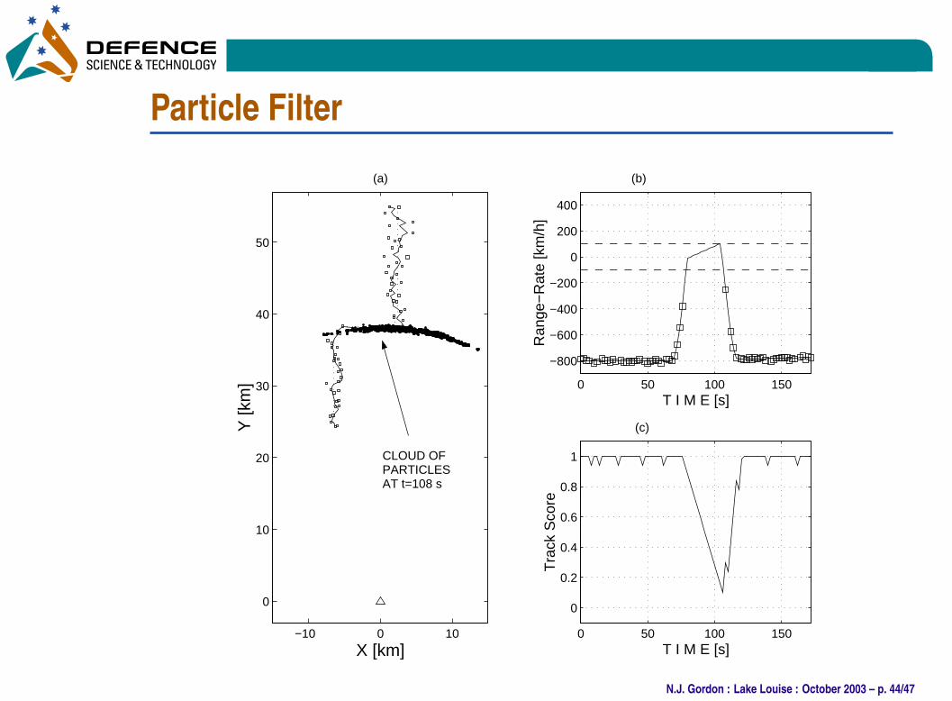
•
Particle Filter
−10 0 10
0
10
20
30
40
50
X [km]
Y [k
m]
(a)
0 50 100 150
−800
−600
−400
−200
0
200
400
T I M E [s]
Ran
ge−
Rat
e [k
m/h
]
(b)
0 50 100 150
0
0.2
0.4
0.6
0.8
1
T I M E [s]
Tra
ck S
core
(c)
CLOUD OF PARTICLESAT t=108 s
N.J. Gordon : Lake Louise : October 2003 – p. 44/47
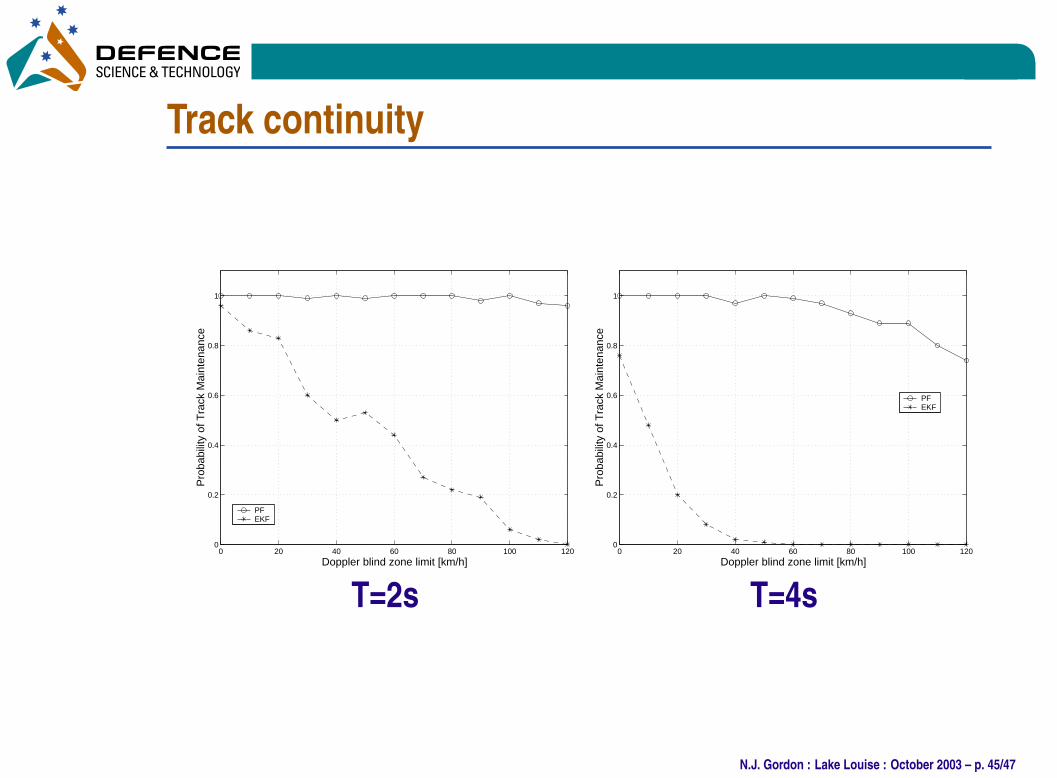
•
Track continuity
0 20 40 60 80 100 1200
0.2
0.4
0.6
0.8
1
Doppler blind zone limit [km/h]
Pro
babi
lity
of T
rack
Mai
nten
ance
PF EKF
T=2s
0 20 40 60 80 100 1200
0.2
0.4
0.6
0.8
1
Doppler blind zone limit [km/h]
Pro
babi
lity
of T
rack
Mai
nten
ance
PF EKF
T=4s
N.J. Gordon : Lake Louise : October 2003 – p. 45/47
•
Problems hindering SMC
– Convergence results
– Becoming available (Del Moral, Crisan, Chopin, Lyons, Doucet ...)
– Communication bandwidth
– Large particle sets impossible to send
– Interoperability
– Need to integrate with varied tracking algorithms
– Computation
– Expensive so look to minimise Monte Carlo
– Multi-target problems
– Rao-Blackwellisation
N.J. Gordon : Lake Louise : October 2003 – p. 46/47
•
Final comments
– Sequential Monte Carlo methods
– “Optimal” filtering for nonlinear/non Gaussian
models
– Flexible/Parallelizable
– Not a black-box: efficiency depends on careful
design.
– If the Kalman filter is appropriate for your application
use it
– A Kalman filter is a (one) particle filter
N.J. Gordon : Lake Louise : October 2003 – p. 47/47