Beyond Multilevel Regression Modeling:Multilevel Analysis in a General Latent

Variable Framework

Bengt Muthen & Tihomir Asparouhov∗

To appear in The Handbook of Advanced Multilevel Analysis.J. Hox & J.K Roberts (eds), Taylor and Francis

January 23, 2009

∗This paper builds on a presentation by the first author at the AERA HLM SIG, SanFrancisco, April 8, 2006. The research of the first author was supported by grant R21AA10948-01A1 from the NIAAA, by NIMH under grant No. MH40859, and by grantP30 MH066247 from the NIDA and the NIMH. We thank Kristopher Preacher for helpfulcomments.

1

Abstract

Multilevel modeling is often treated as if it concerns only regressionanalysis and growth modeling. Multilevel modeling, however, is rele-vant for nested data not only with regression and growth analysis butwith all types of statistical analyses. This chapter has two aims. First,it shows that already in the traditional multilevel analysis areas of re-gression and growth there are several new modeling opportunities thatshould be considered. Second, it gives an overview with examples ofmultilevel modeling for path analysis, factor analysis, structural equa-tion modeling, and growth mixture modeling. Examples include twoextensions of two-level regression analysis with measurement error inthe level 2 covariate and a level 1 mixture; two-level path analysis andstructural equation modeling; two-level exploratory factor analysis ofclassroom misbehavior; two-level growth modeling using a two-partmodel for heavy drinking development; an unconventional approachto three-level growth modeling of math achievement; and multilevellatent class mediation of high school dropout using multilevel growthmixture modeling of math achievement development.

2

1 Introduction

Multilevel modeling is often treated as if it concerns only regressionanalysis and growth modeling (Raudenbush & Bryk, 2002; Snijders& Bosker, 1999). Furthermore, growth modeling is merely seen as avariation on the regression theme, regressing the outcome on a time-related covariate. Multilevel modeling, however, is relevant for nesteddata not only with regression analysis but with all types of statisticalanalyses, including

• Regression analysis

• Path analysis

• Factor analysis

• Structural equation modeling

• Growth modeling

• Survival analysis

• Latent class analysis

• Latent transition analysis

• Growth mixture modeling

This chapter has two aims. First, it shows that already in the tradi-tional multilevel analysis areas of regression and growth there are sev-eral new modeling opportunities that should be considered. Second,it gives an overview with examples of multilevel modeling for pathanalysis, factor analysis, structural equation modeling, and growthmixture modeling. Due to lack of space, survival, latent class, andlatent transition analysis are not covered. All of these topics, how-ever, are covered within the latent variable framework of the Mplussoftware, which is the basis for this chapter. A technical descriptionof this framework including not only multilevel features but also finitemixtures is given in Muthen and Asparouhov (2008). Survival mixtureanalysis is discussed in Asparouhov, Masyn and Muthen (2006). Seealso examples in the Mplus User’s Guide (Muthen & Muthen, 2008).The User’s Guide is available online at www.statmodel.com.

The outline of the chapter is as follows. Section 2 discusses two ex-tensions of two-level regression analysis, Section 3 discusses two-levelpath analysis and structural equation modeling, Section 4 presents anexample of two-level exploratory factor analysis, Section 5 discussestwo-level growth modeling using a two-part model, Section 6 discusses

3

an unconventional approach to three-level growth modeling, and Sec-tion 7 presents an example of multilevel growth mixture modeling.

2 Two-level regression

One may ask if there really is anything new that can be said aboutmultilevel regression. The answer, surprisingly, is yes. Two extensionsof conventional two-level regression analysis will be discussed here,taking into account measurement error in covariates and taking intoaccount unobserved heterogeneity among level 1 subjects.

2.1 Measurement error in covariates

It is well known that measurement error in covariates creates biasedregression slopes. In multilevel regression a particularly critical covari-ate is the level 2 covariate x.j , drawing on information from individualswithin clusters to reflect cluster characteristics, as for example withstudents rating the school environment. Based on relatively few stu-dents such covariates may contain a considerable amount of measure-ment error, but this fact seems to not have gained widespread recogni-tion in multilevel regression modeling. The following discussion drawson Asparouhov and Muthen (2006) and Ludtke et al (2008). The topicseems to be rediscovered every two decades given earlier contributionsby Schmidt (1969) and Muthen (1989).

Raudenbush and Bryk (2002; p. 140, Table 5.11) considered thetwo-level, random intercept, group-centered regression model

yij = β0j + β1j (xij − x.j) + rij , (1)β0j = γ00 + γ01 x.j + uj , (2)β1j = γ10, (3)

defining the “contextual effect” as

βc = γ01 − γ10. (4)

Often, x.j can be seen as an estimate of a level 2 construct which hasnot been directly measured. In fact, the covariates (xij − x.j) and x.j

may be seen as proxies for latent covariates (cf Asparouhov & Muthen,2006),

xij − x.j ≈ xijw, (5)x.j ≈ xjb, (6)

4

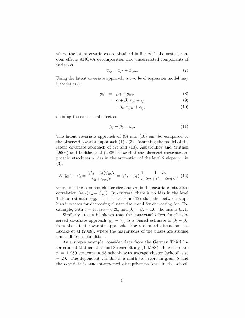
where the latent covariates are obtained in line with the nested, ran-dom effects ANOVA decomposition into uncorrelated components ofvariation,

xij = xjb + xijw. (7)

Using the latent covariate approach, a two-level regression model maybe written as

yij = yjb + yijw (8)= α+ βb xjb + εj (9)

+βw xijw + εij , (10)

defining the contextual effect as

βc = βb − βw. (11)

The latent covariate approach of (9) and (10) can be compared tothe observed covariate approach (1) - (3). Assuming the model of thelatent covariate approach of (9) and (10), Asparouhov and Muthen(2006) and Ludtke et al (2008) show that the observed covariate ap-proach introduces a bias in the estimation of the level 2 slope γ01 in(3),

E(γ01)− βb =(βw − βb)ψw/c

ψb + ψw/c= (βw − βb)

1c

1− iccicc+ (1− icc)/c

, (12)

where c is the common cluster size and icc is the covariate intraclasscorrelation (ψb/(ψb + ψw)). In contrast, there is no bias in the level1 slope estimate γ10. It is clear from (12) that the between slopebias increases for decreasing cluster size c and for decreasing icc. Forexample, with c = 15, icc = 0.20, and βw − βb = 1.0, the bias is 0.21.

Similarly, it can be shown that the contextual effect for the ob-served covariate approach γ01 − γ10 is a biased estimate of βb − βw

from the latent covariate approach. For a detailed discussion, seeLudtke et al (2008), where the magnitudes of the biases are studiedunder different conditions.

As a simple example, consider data from the German Third In-ternational Mathematics and Science Study (TIMSS). Here there aren = 1, 980 students in 98 schools with average cluster (school) size= 20. The dependent variable is a math test score in grade 8 andthe covariate is student-reported disruptiveness level in the school.

5

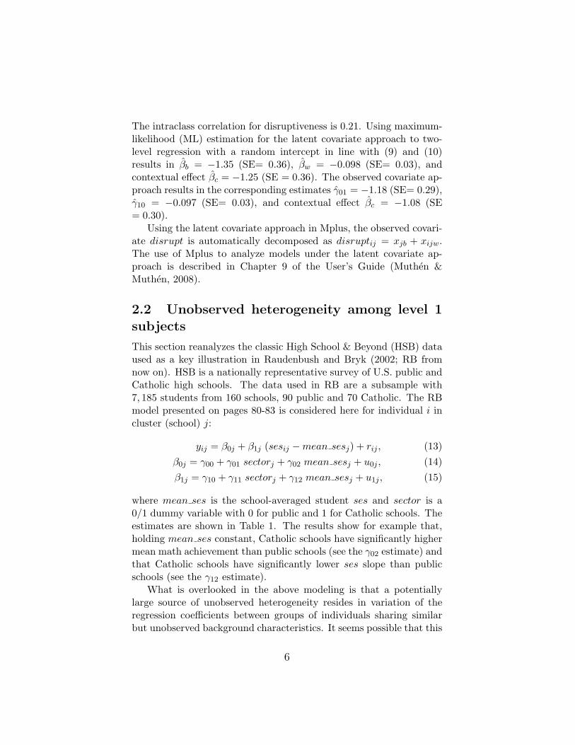
The intraclass correlation for disruptiveness is 0.21. Using maximum-likelihood (ML) estimation for the latent covariate approach to two-level regression with a random intercept in line with (9) and (10)results in βb = −1.35 (SE= 0.36), βw = −0.098 (SE= 0.03), andcontextual effect βc = −1.25 (SE = 0.36). The observed covariate ap-proach results in the corresponding estimates γ01 = −1.18 (SE= 0.29),γ10 = −0.097 (SE= 0.03), and contextual effect βc = −1.08 (SE= 0.30).

Using the latent covariate approach in Mplus, the observed covari-ate disrupt is automatically decomposed as disruptij = xjb + xijw.The use of Mplus to analyze models under the latent covariate ap-proach is described in Chapter 9 of the User’s Guide (Muthen &Muthen, 2008).

2.2 Unobserved heterogeneity among level 1subjects

This section reanalyzes the classic High School & Beyond (HSB) dataused as a key illustration in Raudenbush and Bryk (2002; RB fromnow on). HSB is a nationally representative survey of U.S. public andCatholic high schools. The data used in RB are a subsample with7, 185 students from 160 schools, 90 public and 70 Catholic. The RBmodel presented on pages 80-83 is considered here for individual i incluster (school) j:

yij = β0j + β1j (sesij −mean sesj) + rij , (13)β0j = γ00 + γ01 sectorj + γ02 mean sesj + u0j , (14)β1j = γ10 + γ11 sectorj + γ12 mean sesj + u1j , (15)

where mean ses is the school-averaged student ses and sector is a0/1 dummy variable with 0 for public and 1 for Catholic schools. Theestimates are shown in Table 1. The results show for example that,holding mean ses constant, Catholic schools have significantly highermean math achievement than public schools (see the γ02 estimate) andthat Catholic schools have significantly lower ses slope than publicschools (see the γ12 estimate).

What is overlooked in the above modeling is that a potentiallylarge source of unobserved heterogeneity resides in variation of theregression coefficients between groups of individuals sharing similarbut unobserved background characteristics. It seems possible that this

6

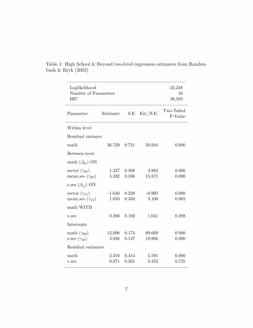
Table 1: High School & Beyond two-level regression estimates from Rauden-bush & Bryk (2002)

Loglikelihood -23,248Number of Parameters 10BIC 46,585

Parameter Estimate S.E Est./S.E.Two-Tailed

P-Value

Within level

Residual variance

math 36.720 0.721 50.944 0.000

Between level

math (β0j) ON

sector (γ01) 1.227 0.308 3.982 0.000mean ses (γ02) 5.332 0.336 15.871 0.000

s ses (β1j) ON

sector (γ11) -1.640 0.238 -6.905 0.000mean ses (γ12) 1.033 0.333 3.100 0.002

math WITH

s ses 0.200 0.192 1.041 0.298

Intercepts

math (γ00) 12.096 0.174 69.669 0.000s ses (γ10) 2.938 0.147 19.986 0.000

Residual variances

math 2.316 0.414 5.591 0.000s ses 0.071 0.201 0.352 0.725

7

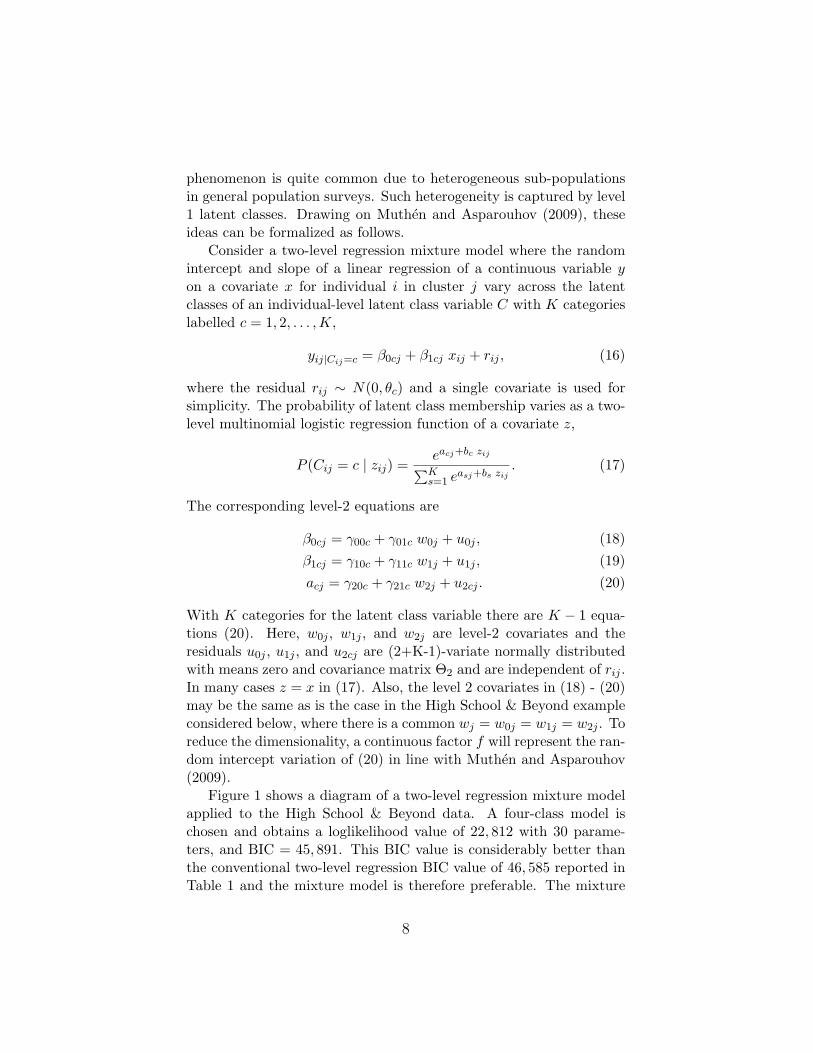
phenomenon is quite common due to heterogeneous sub-populationsin general population surveys. Such heterogeneity is captured by level1 latent classes. Drawing on Muthen and Asparouhov (2009), theseideas can be formalized as follows.

Consider a two-level regression mixture model where the randomintercept and slope of a linear regression of a continuous variable yon a covariate x for individual i in cluster j vary across the latentclasses of an individual-level latent class variable C with K categorieslabelled c = 1, 2, . . . ,K,

yij|Cij=c = β0cj + β1cj xij + rij , (16)

where the residual rij ∼ N(0, θc) and a single covariate is used forsimplicity. The probability of latent class membership varies as a two-level multinomial logistic regression function of a covariate z,

P (Cij = c | zij) =eacj+bc zij∑K

s=1 easj+bs zij

. (17)

The corresponding level-2 equations are

β0cj = γ00c + γ01c w0j + u0j , (18)β1cj = γ10c + γ11c w1j + u1j , (19)acj = γ20c + γ21c w2j + u2cj . (20)

With K categories for the latent class variable there are K − 1 equa-tions (20). Here, w0j , w1j , and w2j are level-2 covariates and theresiduals u0j , u1j , and u2cj are (2+K-1)-variate normally distributedwith means zero and covariance matrix Θ2 and are independent of rij .In many cases z = x in (17). Also, the level 2 covariates in (18) - (20)may be the same as is the case in the High School & Beyond exampleconsidered below, where there is a common wj = w0j = w1j = w2j . Toreduce the dimensionality, a continuous factor f will represent the ran-dom intercept variation of (20) in line with Muthen and Asparouhov(2009).

Figure 1 shows a diagram of a two-level regression mixture modelapplied to the High School & Beyond data. A four-class model ischosen and obtains a loglikelihood value of 22, 812 with 30 parame-ters, and BIC = 45, 891. This BIC value is considerably better thanthe conventional two-level regression BIC value of 46, 585 reported inTable 1 and the mixture model is therefore preferable. The mixture

8

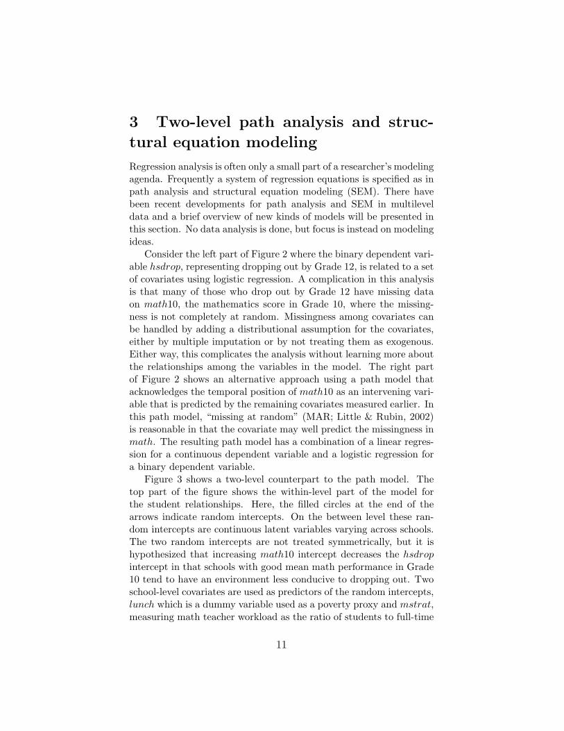
model and its ML estimates can be interpreted as follows. Becausethis type of model is new to readers, Figure 1 will be used to under-stand the estimates rather than reporting a table of the parameterestimates for (16) - (20).

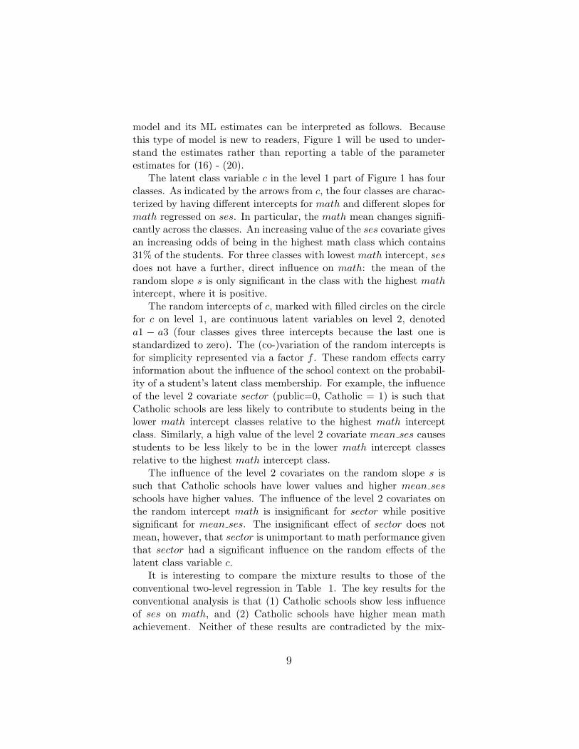
The latent class variable c in the level 1 part of Figure 1 has fourclasses. As indicated by the arrows from c, the four classes are charac-terized by having different intercepts for math and different slopes formath regressed on ses. In particular, the math mean changes signifi-cantly across the classes. An increasing value of the ses covariate givesan increasing odds of being in the highest math class which contains31% of the students. For three classes with lowest math intercept, sesdoes not have a further, direct influence on math: the mean of therandom slope s is only significant in the class with the highest mathintercept, where it is positive.

The random intercepts of c, marked with filled circles on the circlefor c on level 1, are continuous latent variables on level 2, denoteda1 − a3 (four classes gives three intercepts because the last one isstandardized to zero). The (co-)variation of the random intercepts isfor simplicity represented via a factor f . These random effects carryinformation about the influence of the school context on the probabil-ity of a student’s latent class membership. For example, the influenceof the level 2 covariate sector (public=0, Catholic = 1) is such thatCatholic schools are less likely to contribute to students being in thelower math intercept classes relative to the highest math interceptclass. Similarly, a high value of the level 2 covariate mean ses causesstudents to be less likely to be in the lower math intercept classesrelative to the highest math intercept class.

The influence of the level 2 covariates on the random slope s issuch that Catholic schools have lower values and higher mean sesschools have higher values. The influence of the level 2 covariates onthe random intercept math is insignificant for sector while positivesignificant for mean ses. The insignificant effect of sector does notmean, however, that sector is unimportant to math performance giventhat sector had a significant influence on the random effects of thelatent class variable c.

It is interesting to compare the mixture results to those of theconventional two-level regression in Table 1. The key results for theconventional analysis is that (1) Catholic schools show less influenceof ses on math, and (2) Catholic schools have higher mean mathachievement. Neither of these results are contradicted by the mix-

9

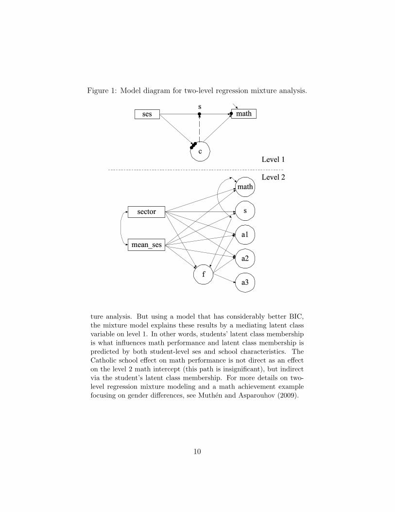
Figure 1: Model diagram for two-level regression mixture analysis.

ture analysis. But using a model that has considerably better BIC,the mixture model explains these results by a mediating latent classvariable on level 1. In other words, students’ latent class membershipis what influences math performance and latent class membership ispredicted by both student-level ses and school characteristics. TheCatholic school effect on math performance is not direct as an effecton the level 2 math intercept (this path is insignificant), but indirectvia the student’s latent class membership. For more details on two-level regression mixture modeling and a math achievement examplefocusing on gender differences, see Muthen and Asparouhov (2009).

10

3 Two-level path analysis and struc-

tural equation modeling

Regression analysis is often only a small part of a researcher’s modelingagenda. Frequently a system of regression equations is specified as inpath analysis and structural equation modeling (SEM). There havebeen recent developments for path analysis and SEM in multileveldata and a brief overview of new kinds of models will be presented inthis section. No data analysis is done, but focus is instead on modelingideas.

Consider the left part of Figure 2 where the binary dependent vari-able hsdrop, representing dropping out by Grade 12, is related to a setof covariates using logistic regression. A complication in this analysisis that many of those who drop out by Grade 12 have missing dataon math10, the mathematics score in Grade 10, where the missing-ness is not completely at random. Missingness among covariates canbe handled by adding a distributional assumption for the covariates,either by multiple imputation or by not treating them as exogenous.Either way, this complicates the analysis without learning more aboutthe relationships among the variables in the model. The right partof Figure 2 shows an alternative approach using a path model thatacknowledges the temporal position of math10 as an intervening vari-able that is predicted by the remaining covariates measured earlier. Inthis path model, “missing at random” (MAR; Little & Rubin, 2002)is reasonable in that the covariate may well predict the missingness inmath. The resulting path model has a combination of a linear regres-sion for a continuous dependent variable and a logistic regression fora binary dependent variable.

Figure 3 shows a two-level counterpart to the path model. Thetop part of the figure shows the within-level part of the model forthe student relationships. Here, the filled circles at the end of thearrows indicate random intercepts. On the between level these ran-dom intercepts are continuous latent variables varying across schools.The two random intercepts are not treated symmetrically, but it ishypothesized that increasing math10 intercept decreases the hsdropintercept in that schools with good mean math performance in Grade10 tend to have an environment less conducive to dropping out. Twoschool-level covariates are used as predictors of the random intercepts,lunch which is a dummy variable used as a poverty proxy and mstrat,measuring math teacher workload as the ratio of students to full-time

11

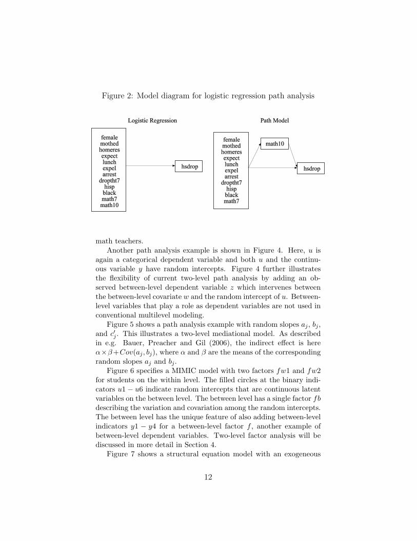
Figure 2: Model diagram for logistic regression path analysis

math teachers.Another path analysis example is shown in Figure 4. Here, u is

again a categorical dependent variable and both u and the continu-ous variable y have random intercepts. Figure 4 further illustratesthe flexibility of current two-level path analysis by adding an ob-served between-level dependent variable z which intervenes betweenthe between-level covariate w and the random intercept of u. Between-level variables that play a role as dependent variables are not used inconventional multilevel modeling.

Figure 5 shows a path analysis example with random slopes aj , bj ,and c′j . This illustrates a two-level mediational model. As describedin e.g. Bauer, Preacher and Gil (2006), the indirect effect is hereα×β+Cov(aj , bj), where α and β are the means of the correspondingrandom slopes aj and bj .

Figure 6 specifies a MIMIC model with two factors fw1 and fw2for students on the within level. The filled circles at the binary indi-cators u1 − u6 indicate random intercepts that are continuous latentvariables on the between level. The between level has a single factor fbdescribing the variation and covariation among the random intercepts.The between level has the unique feature of also adding between-levelindicators y1 − y4 for a between-level factor f , another example ofbetween-level dependent variables. Two-level factor analysis will bediscussed in more detail in Section 4.

Figure 7 shows a structural equation model with an exogeneous

12

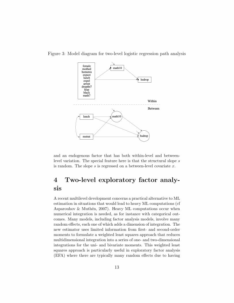
Figure 3: Model diagram for two-level logistic regression path analysis

and an endogenous factor that has both within-level and between-level variation. The special feature here is that the structural slope sis random. The slope s is regressed on a between-level covariate x.

4 Two-level exploratory factor analy-

sis

A recent multilevel development concerns a practical alternative to MLestimation in situations that would lead to heavy ML computations (cfAsparouhov & Muthen, 2007). Heavy ML computations occur whennumerical integration is needed, as for instance with categorical out-comes. Many models, including factor analysis models, involve manyrandom effects, each one of which adds a dimension of integration. Thenew estimator uses limited information from first- and second-ordermoments to formulate a weighted least squares approach that reducesmultidimensional integration into a series of one- and two-dimensionalintegrations for the uni- and bivariate moments. This weighted leastsquares approach is particularly useful in exploratory factor analysis(EFA) where there are typically many random effects due to having

13

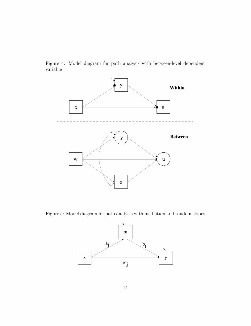
Figure 4: Model diagram for path analysis with between-level dependentvariable

Figure 5: Model diagram for path analysis with mediation and random slopes

14

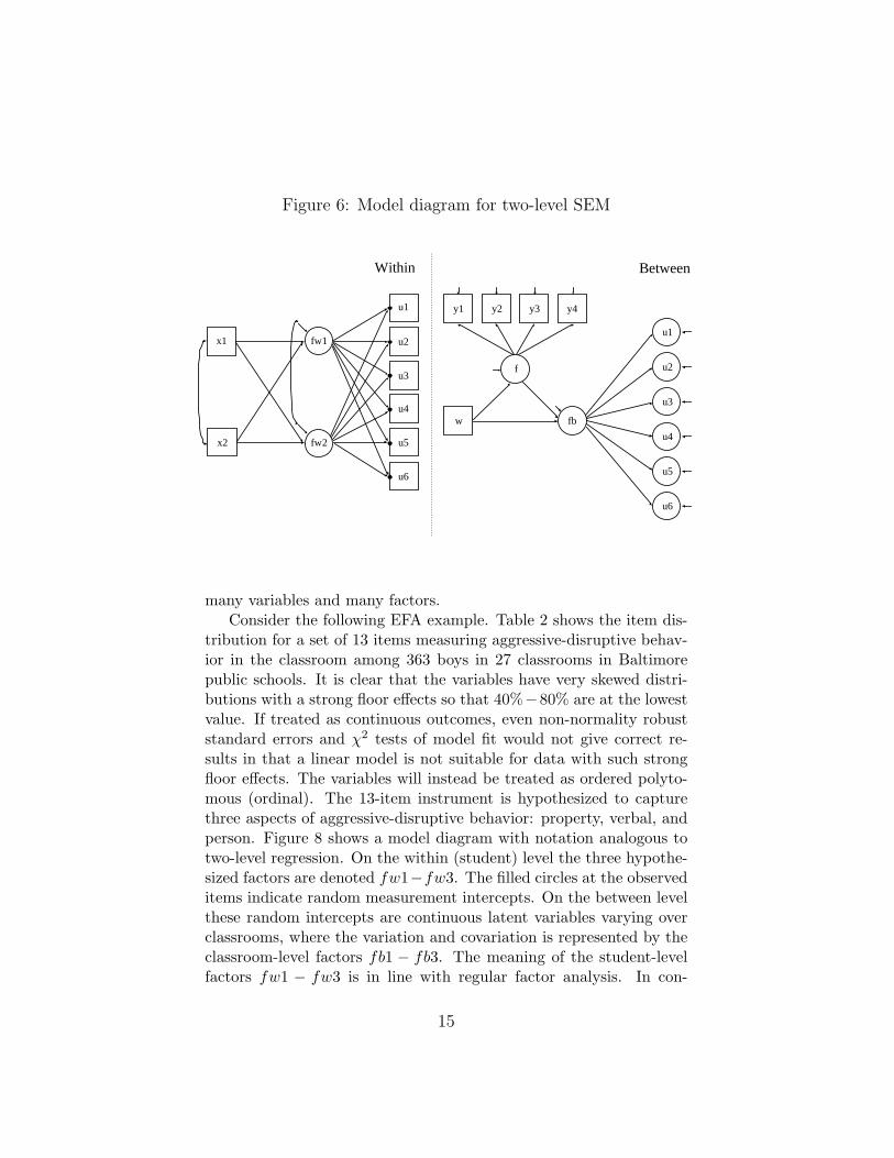
Figure 6: Model diagram for two-level SEM

x1

x2

u1

u2

u3

u4

u5

u6

fw1

fw2

y1 y2 y3 y4

f

w fb

u1

u2

u3

u4

u5

u6

Within Between

many variables and many factors.Consider the following EFA example. Table 2 shows the item dis-

tribution for a set of 13 items measuring aggressive-disruptive behav-ior in the classroom among 363 boys in 27 classrooms in Baltimorepublic schools. It is clear that the variables have very skewed distri-butions with a strong floor effects so that 40%−80% are at the lowestvalue. If treated as continuous outcomes, even non-normality robuststandard errors and χ2 tests of model fit would not give correct re-sults in that a linear model is not suitable for data with such strongfloor effects. The variables will instead be treated as ordered polyto-mous (ordinal). The 13-item instrument is hypothesized to capturethree aspects of aggressive-disruptive behavior: property, verbal, andperson. Figure 8 shows a model diagram with notation analogous totwo-level regression. On the within (student) level the three hypothe-sized factors are denoted fw1−fw3. The filled circles at the observeditems indicate random measurement intercepts. On the between levelthese random intercepts are continuous latent variables varying overclassrooms, where the variation and covariation is represented by theclassroom-level factors fb1 − fb3. The meaning of the student-levelfactors fw1 − fw3 is in line with regular factor analysis. In con-

15

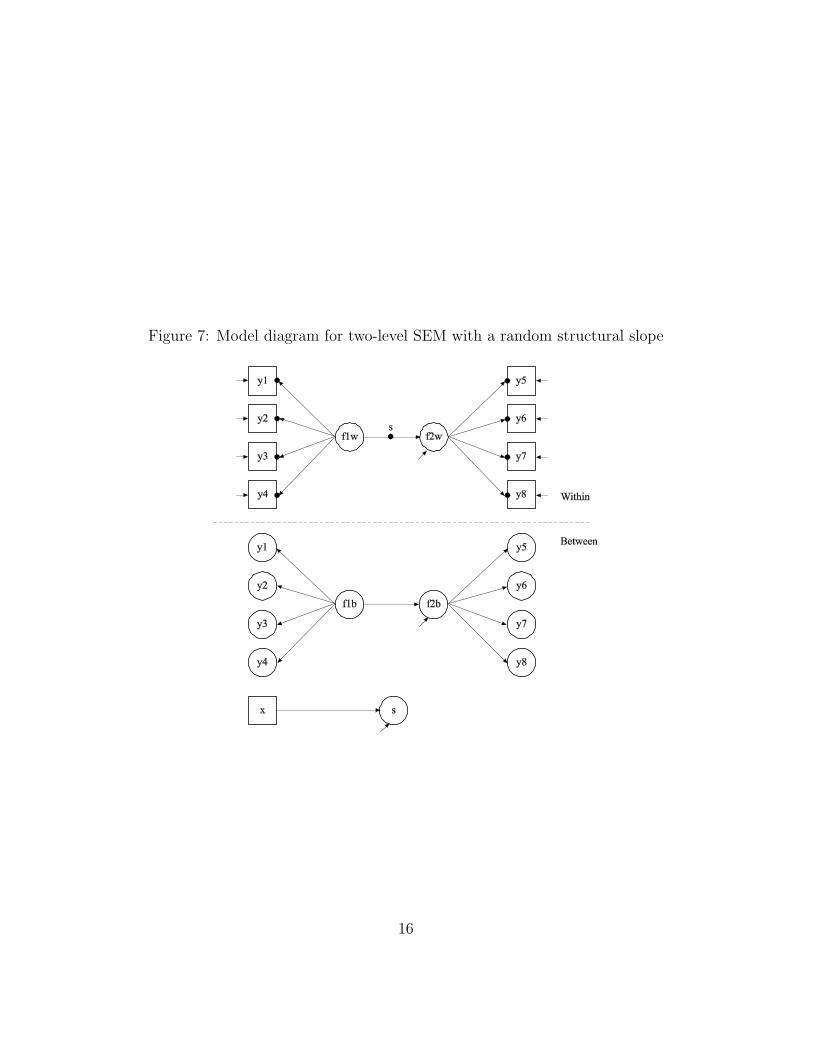
Figure 7: Model diagram for two-level SEM with a random structural slope

16

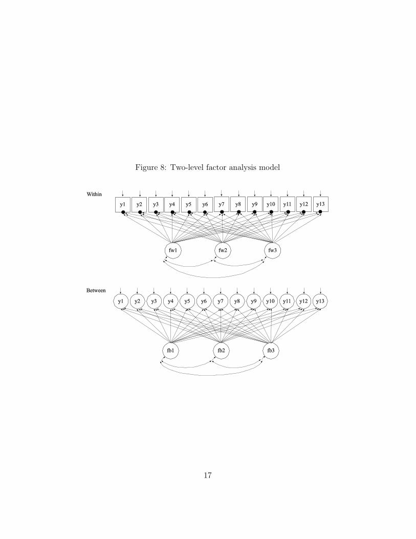
Figure 8: Two-level factor analysis model

17

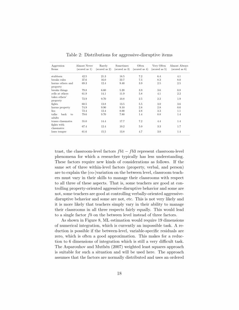
Table 2: Distributions for aggressive-disruptive items

Aggression Almost Never Rarely Sometimes Often Very Often Almost AlwaysItems (scored as 1) (scored as 2) (scored as 3) (scored as 4) (scored as 5) (scored as 6)

stubborn 42.5 21.3 18.5 7.2 6.4 4.1breaks rules 37.6 16.0 22.7 7.5 8.3 8.0harms others andproperty

69.3 12.4 9.40 3.9 2.5 2.5

breaks things 79.8 6.60 5.20 3.9 3.6 0.8yells at others 61.9 14.1 11.9 5.8 4.1 2.2takes others’

72.9 9.70 10.8 2.5 2.2 1.9propertyfights 60.5 13.8 13.5 5.5 3.0 3.6harms property 74.9 9.90 9.10 2.8 2.8 0.6lies 72.4 12.4 8.00 2.8 3.3 1.1talks back toadults

79.6 9.70 7.80 1.4 0.8 1.4

teases classmates 55.0 14.4 17.7 7.2 4.4 1.4fights with

67.4 12.4 10.2 5.0 3.3 1.7classmatesloses temper 61.6 15.5 13.8 4.7 3.0 1.4

trast, the classroom-level factors fb1 − fb3 represent classroom-levelphenomena for which a researcher typically has less understanding.These factors require new kinds of considerations as follows. If thesame set of three within-level factors (property, verbal, and person)are to explain the (co-)variation on the between level, classroom teach-ers must vary in their skills to manage their classrooms with respectto all three of these aspects. That is, some teachers are good at con-trolling property-oriented aggressive-disruptive behavior and some arenot, some teachers are good at controlling verbally-oriented aggressive-disruptive behavior and some are not, etc. This is not very likely andit is more likely that teachers simply vary in their ability to managetheir classrooms in all three respects fairly equally. This would leadto a single factor fb on the between level instead of three factors.

As shown in Figure 8, ML estimation would require 19 dimensionsof numerical integration, which is currently an impossible task. A re-duction is possible if the between-level, variable-specific residuals arezero, which is often a good approximation. This makes for a reduc-tion to 6 dimensions of integration which is still a very difficult task.The Asparouhov and Muthen (2007) weighted least squares approachis suitable for such a situation and will be used here. The approachassumes that the factors are normally distributed and uses an ordered

18

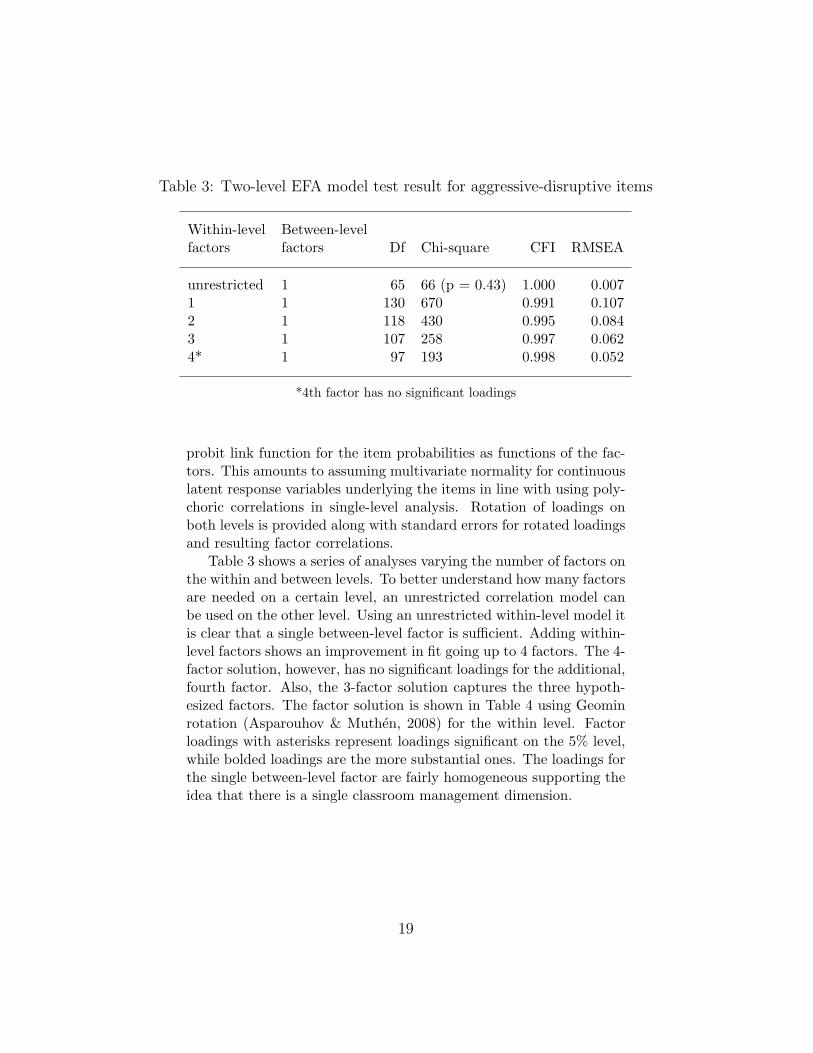
Table 3: Two-level EFA model test result for aggressive-disruptive items

Within-level Between-levelfactors factors Df Chi-square CFI RMSEA

unrestricted 1 65 66 (p = 0.43) 1.000 0.0071 1 130 670 0.991 0.1072 1 118 430 0.995 0.0843 1 107 258 0.997 0.0624* 1 97 193 0.998 0.052

*4th factor has no significant loadings

probit link function for the item probabilities as functions of the fac-tors. This amounts to assuming multivariate normality for continuouslatent response variables underlying the items in line with using poly-choric correlations in single-level analysis. Rotation of loadings onboth levels is provided along with standard errors for rotated loadingsand resulting factor correlations.

Table 3 shows a series of analyses varying the number of factors onthe within and between levels. To better understand how many factorsare needed on a certain level, an unrestricted correlation model canbe used on the other level. Using an unrestricted within-level model itis clear that a single between-level factor is sufficient. Adding within-level factors shows an improvement in fit going up to 4 factors. The 4-factor solution, however, has no significant loadings for the additional,fourth factor. Also, the 3-factor solution captures the three hypoth-esized factors. The factor solution is shown in Table 4 using Geominrotation (Asparouhov & Muthen, 2008) for the within level. Factorloadings with asterisks represent loadings significant on the 5% level,while bolded loadings are the more substantial ones. The loadings forthe single between-level factor are fairly homogeneous supporting theidea that there is a single classroom management dimension.

19

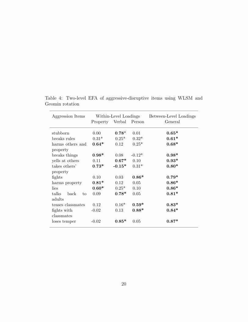
Table 4: Two-level EFA of aggressive-disruptive items using WLSM andGeomin rotation

Aggression Items Within-Level Loadings Between-Level LoadingsProperty Verbal Person General

stubborn 0.00 0.78* 0.01 0.65*breaks rules 0.31* 0.25* 0.32* 0.61*harms others andproperty

0.64* 0.12 0.25* 0.68*

breaks things 0.98* 0.08 -0.12* 0.98*yells at others 0.11 0.67* 0.10 0.93*takes others’ 0.73* -0.15* 0.31* 0.80*propertyfights 0.10 0.03 0.86* 0.79*harms property 0.81* 0.12 0.05 0.86*lies 0.60* 0.25* 0.10 0.86*talks back toadults

0.09 0.78* 0.05 0.81*

teases classmates 0.12 0.16* 0.59* 0.83*fights with -0.02 0.13 0.88* 0.84*classmatesloses temper -0.02 0.85* 0.05 0.87*

20

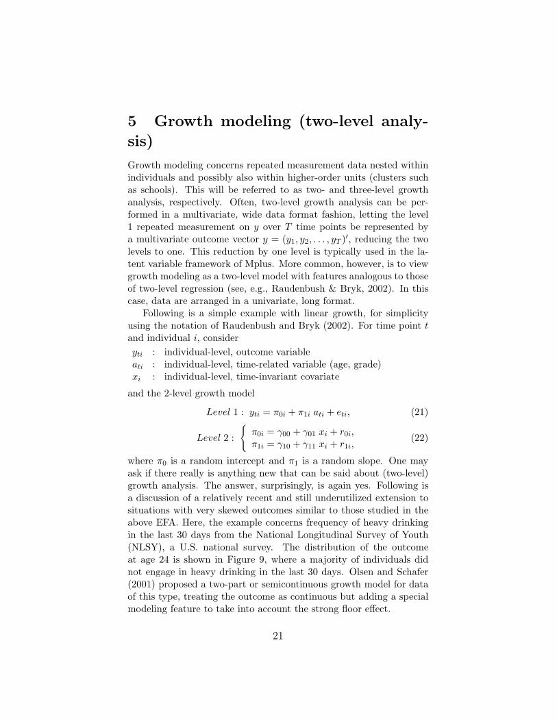
5 Growth modeling (two-level analy-

sis)

Growth modeling concerns repeated measurement data nested withinindividuals and possibly also within higher-order units (clusters suchas schools). This will be referred to as two- and three-level growthanalysis, respectively. Often, two-level growth analysis can be per-formed in a multivariate, wide data format fashion, letting the level1 repeated measurement on y over T time points be represented bya multivariate outcome vector y = (y1, y2, . . . , yT )′, reducing the twolevels to one. This reduction by one level is typically used in the la-tent variable framework of Mplus. More common, however, is to viewgrowth modeling as a two-level model with features analogous to thoseof two-level regression (see, e.g., Raudenbush & Bryk, 2002). In thiscase, data are arranged in a univariate, long format.

Following is a simple example with linear growth, for simplicityusing the notation of Raudenbush and Bryk (2002). For time point tand individual i, consideryti : individual-level, outcome variableati : individual-level, time-related variable (age, grade)xi : individual-level, time-invariant covariate

and the 2-level growth model

Level 1 : yti = π0i + π1i ati + eti, (21)

Level 2 :

{π0i = γ00 + γ01 xi + r0i,π1i = γ10 + γ11 xi + r1i,

(22)

where π0 is a random intercept and π1 is a random slope. One mayask if there really is anything new that can be said about (two-level)growth analysis. The answer, surprisingly, is again yes. Following isa discussion of a relatively recent and still underutilized extension tosituations with very skewed outcomes similar to those studied in theabove EFA. Here, the example concerns frequency of heavy drinkingin the last 30 days from the National Longitudinal Survey of Youth(NLSY), a U.S. national survey. The distribution of the outcomeat age 24 is shown in Figure 9, where a majority of individuals didnot engage in heavy drinking in the last 30 days. Olsen and Schafer(2001) proposed a two-part or semicontinuous growth model for dataof this type, treating the outcome as continuous but adding a specialmodeling feature to take into account the strong floor effect.

21

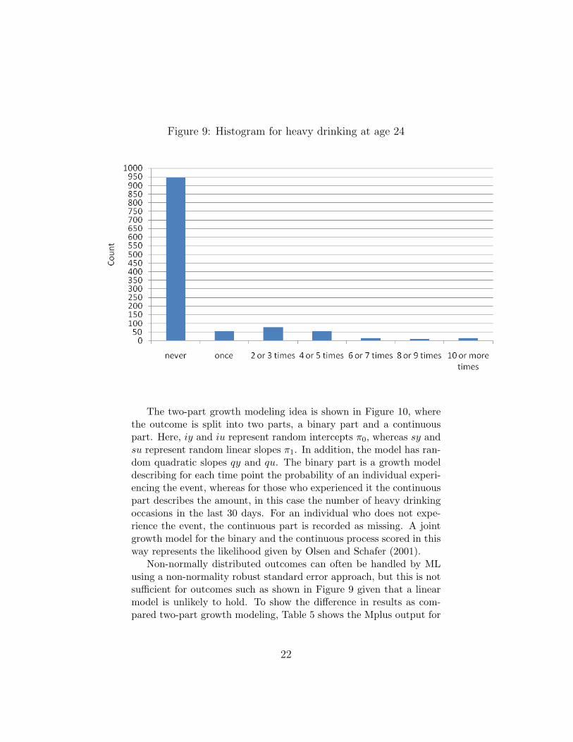
Figure 9: Histogram for heavy drinking at age 24

The two-part growth modeling idea is shown in Figure 10, where

the outcome is split into two parts, a binary part and a continuouspart. Here, iy and iu represent random intercepts π0, whereas sy andsu represent random linear slopes π1. In addition, the model has ran-dom quadratic slopes qy and qu. The binary part is a growth modeldescribing for each time point the probability of an individual experi-encing the event, whereas for those who experienced it the continuouspart describes the amount, in this case the number of heavy drinkingoccasions in the last 30 days. For an individual who does not expe-rience the event, the continuous part is recorded as missing. A jointgrowth model for the binary and the continuous process scored in thisway represents the likelihood given by Olsen and Schafer (2001).

Non-normally distributed outcomes can often be handled by MLusing a non-normality robust standard error approach, but this is notsufficient for outcomes such as shown in Figure 9 given that a linearmodel is unlikely to hold. To show the difference in results as com-pared two-part growth modeling, Table 5 shows the Mplus output for

22

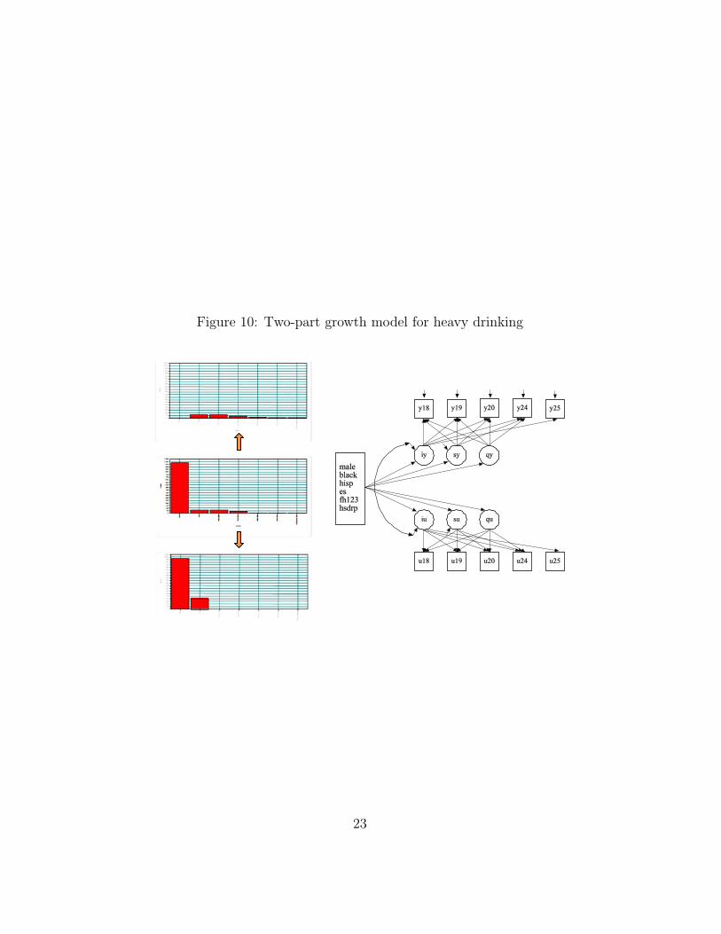
Figure 10: Two-part growth model for heavy drinking

23

the estimated growth model for frequency of heavy drinking ages 18 -25. The results focus on the regression of the random intercept i onthe time-invariant covariates in the model. The time scores are cen-tered at age 25 so that the random intercept refers to the systematicpart of the growth curve at age 25. It is seen that the regular growthmodeling finds all but the last two covariates significant. In contrast,the two-level modeling finds several of the covariates insignificant inone part or the other (the two parts are labeled iy ON for the con-tinuous part and iu ON for the binary part. Consider as an example,the covariate black. As is typically found being black has a signifi-cant negative influence in the regular growth modeling, lowering thefrequency of heavy drinking. In the two-part modeling this covariateis insignificant for the continuous part and significant only for the bi-nary part. This implies that, holding other covariates constant, beingblack significantly lowers the risk of engaging in heavy drinking, butamong blacks who are engaging in heavy drinking there is no differ-ence in amount compared to other ethnic groups. These two paths ofinfluence are confounded in the regular growth modeling.

As shown in Figure 11, a distal outcome can also be added tothe growth model. In this example, the distal outcome is a DSM-based classification into alcohol dependence or not by age 30. Thedistal outcome is predicted by the age 25 random intercept using alogistic regression model part. Table 6 shows that the distal outcomeis significantly influenced only by the age 25-defined random interceptiu for the binary part, not by the random intercept for the continuouspart. In other words, if the probability of engaging in heavy drinkingat age 25 is high the probability of alcohol dependence by age 30is high. But the alcohol dependence probability is not significantlyinfluenced by the frequency of heavy drinking at age 25. The resultsalso show that controlling for age 25 heavy drinking behavior, none ofthe covariates has a significant influence on the distal outcome.

6 Growth modeling (three-level anal-

ysis)

This section considers growth modeling of individual- and cluster-leveldata. A typical example is repeated measures over grades for studentsnested within schools. One may again ask if there really is anythingnew that can be said about growth modeling in cluster data. The

24

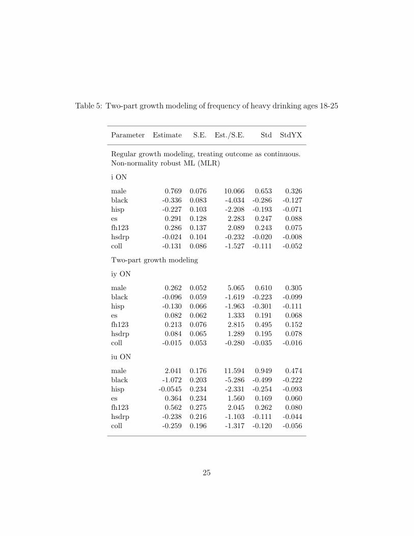
Table 5: Two-part growth modeling of frequency of heavy drinking ages 18-25

Parameter Estimate S.E. Est./S.E. Std StdYX

Regular growth modeling, treating outcome as continuous.Non-normality robust ML (MLR)

i ON

male 0.769 0.076 10.066 0.653 0.326black -0.336 0.083 -4.034 -0.286 -0.127hisp -0.227 0.103 -2.208 -0.193 -0.071es 0.291 0.128 2.283 0.247 0.088fh123 0.286 0.137 2.089 0.243 0.075hsdrp -0.024 0.104 -0.232 -0.020 -0.008coll -0.131 0.086 -1.527 -0.111 -0.052

Two-part growth modeling

iy ON

male 0.262 0.052 5.065 0.610 0.305black -0.096 0.059 -1.619 -0.223 -0.099hisp -0.130 0.066 -1.963 -0.301 -0.111es 0.082 0.062 1.333 0.191 0.068fh123 0.213 0.076 2.815 0.495 0.152hsdrp 0.084 0.065 1.289 0.195 0.078coll -0.015 0.053 -0.280 -0.035 -0.016

iu ON

male 2.041 0.176 11.594 0.949 0.474black -1.072 0.203 -5.286 -0.499 -0.222hisp -0.0545 0.234 -2.331 -0.254 -0.093es 0.364 0.234 1.560 0.169 0.060fh123 0.562 0.275 2.045 0.262 0.080hsdrp -0.238 0.216 -1.103 -0.111 -0.044coll -0.259 0.196 -1.317 -0.120 -0.056

25

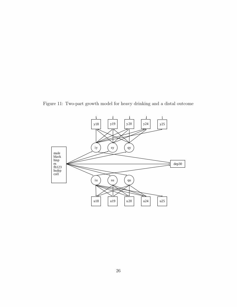
Figure 11: Two-part growth model for heavy drinking and a distal outcome

iu

iy sy

su

maleblackhispesfh123hsdrpcoll

qy

qu

y18 y19 y20 y24 y25

u18 u19 u20 u24 u25

dep30

26

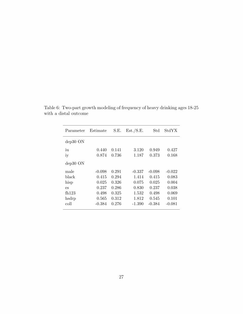
Table 6: Two-part growth modeling of frequency of heavy drinking ages 18-25with a distal outcome

Parameter Estimate S.E. Est./S.E. Std StdYX

dep30 ON

iu 0.440 0.141 3.120 0.949 0.427iy 0.874 0.736 1.187 0.373 0.168

dep30 ON

male -0.098 0.291 -0.337 -0.098 -0.022black 0.415 0.294 1.414 0.415 0.083hisp 0.025 0.326 0.075 0.025 0.004es 0.237 0.286 0.830 0.237 0.038fh123 0.498 0.325 1.532 0.498 0.069hsdrp 0.565 0.312 1.812 0.545 0.101coll -0.384 0.276 -1.390 -0.384 -0.081

27

answer, surprisingly, is once again yes. An important extension tothe conventional 3-level analysis becomes clear when viewed from ageneral latent variable modeling perspective.

For simplicity, the notation will be chosen to coincide with thatof Raudenbush and Bryk (2002). Consider the observed variables fortime point t, individual i, and cluster j,ytij : individual-level, outcome variablea1tij : individual-level, time-related variable (age, grade)a2tij : individual-level, time-varying covariatexij : individual-level, time-invariant covariatewj : cluster-level covariate

and the 3-level growth model

Level 1 : ytij = π0ij + π1ij a1tij + π2tij a2tij + etij , (23)

Level 2 :

π0ij = β00j + β01j xij + r0ij ,π1ij = β10j + β11j xij + r1ij ,π2tij = β20tj + β21tj xij + r2tij ,

(24)

Level 3 :

β00j = γ000 + γ001 wj + u00j ,β10j = γ100 + γ101 wj + u10j ,β20tj = γ200t + γ201t wj + u20tj ,β01j = γ010 + γ011 wj + u01j ,β11j = γ110 + γ111 wj + u11j ,β21tj = γ21t0 + γ21t1 wj + u21tj .

(25)

Here, the πs are random intercepts and slopes varying across individ-uals and clusters, and the βs are random intercepts and slopes varyingacross clusters. The residuals e, r and u are assumed normally dis-tributed with zero means, uncorrelated with respective right-hand sidecovariates, and uncorrelated across levels.

In Mplus, growth modeling in cluster data is represented in a sim-ilar, but slightly different way that offers further modeling flexibility.As mentioned in Section 5 the first difference arises from the level 1repeated measurement on y over time being represented by a mul-tivariate outcome vector y = (y1, y2, . . . , yT )′ so that the number oflevels is reduced from three to two. The second difference is that eachvariable, with the exception of variables multiplied by random slopes,is decomposed into uncorrelated within- and between-cluster compo-nents. Using subscripts w and b to represent within- and between-cluster variation, one may write the variables in (23) as

ytij = ybtj + ywtij , (26)

28

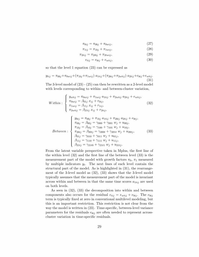
π0ij = π0bj + π0wij , (27)π1ij = π1bj + π1wij , (28)

π2tij = π2tbj + π2twij , (29)etij = ebtj + ewtij , (30)

so that the level 1 equation (23) can be expressed as

ytij = π0bj+π0wij+(π1bj+π1wij) a1tij+(π2btj+π2wtij) a2tij+ebtj+ewtij .(31)

The 3-level model of (23) - (25) can then be rewritten as a 2-level modelwith levels corresponding to within- and between-cluster variation,

Within :

ywtij = π0wij + π1wij a1tij + π2wtij a2tij + ewtij ,π0wij = β01j xij + r0ij ,π1wij = β11j xij + r1ij ,π2wtij = β21tj xij + r2tij ,

(32)

Between :

ybtj = π0bj + π1bj a1tij + π2btj a2tij + ebtj ,π0bj = β00j = γ000 + γ001 wj + u00j ,π1bj = β10j = γ100 + γ101 wj + u10j ,π2btj = β20tj = γ200t + γ201t wj + u20tj ,β01j = γ010 + γ011 wj + u01j ,β11j = γ110 + γ111 wj + u11j ,β21tj = γ21t0 + γ21t1 wj + u21tj .

(33)

From the latent variable perspective taken in Mplus, the first line ofthe within level (32) and the first line of the between level (33) is themeasurement part of the model with growth factors π0, π1 measuredby multiple indicators yt. The next lines of each level contain thestructural part of the model. As is highlighted in (31), the rearrange-ment of the 3-level model as (32), (33) shows that the 3-level modeltypically assumes that the measurement part of the model is invariantacross within and between in that the same time scores a1tij are usedon both levels.

As seen in (32), (33) the decomposition into within and betweencomponents also occurs for the residual etij = ewtij + ebtj . The ebtjterm is typically fixed at zero in conventional multilevel modeling, butthis is an important restriction. This restriction is not clear from theway the model is written in (23). Time-specific, between-level varianceparameters for the residuals ebtj are often needed to represent across-cluster variation in time-specific residuals.

29

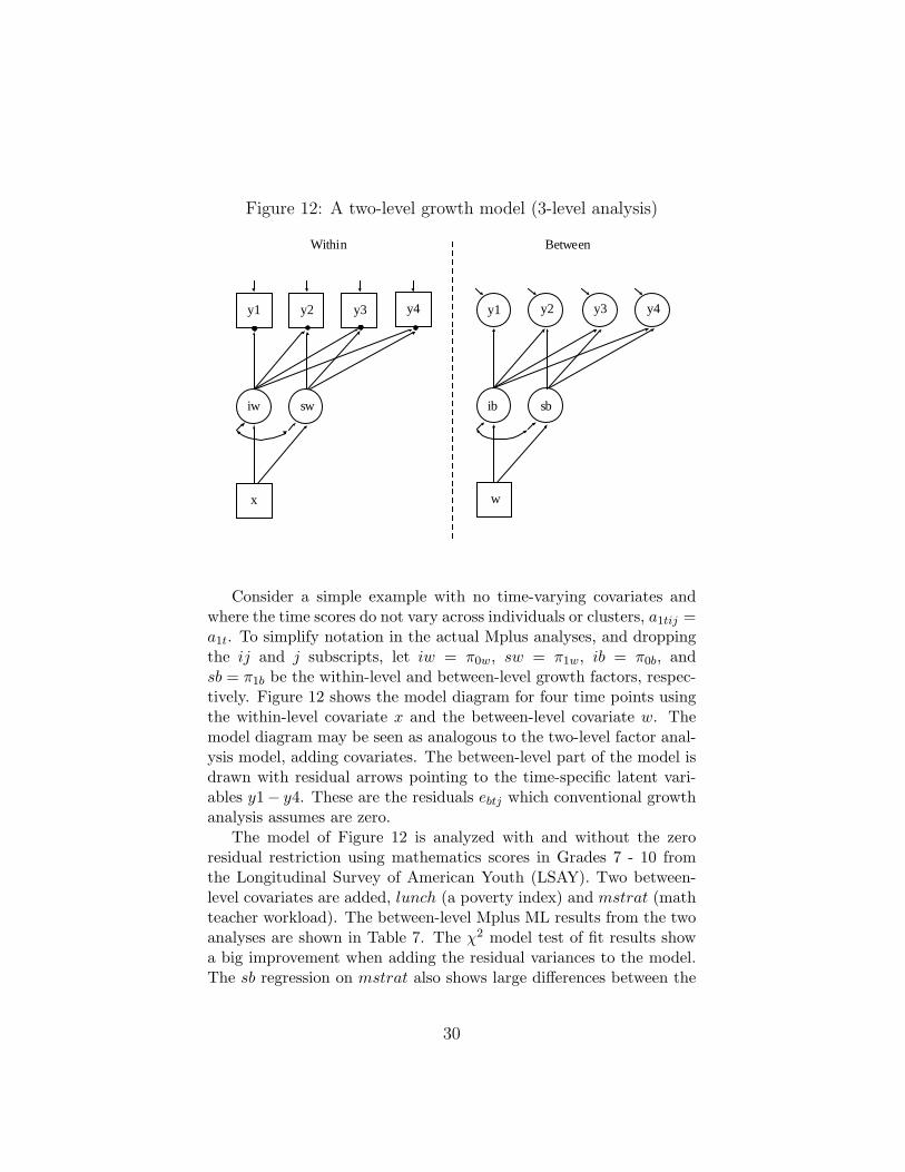
Figure 12: A two-level growth model (3-level analysis)

iw sw

y1 y2 y3 y4

x

ib sb

y1 y2 y3 y4

w

Within Between

Consider a simple example with no time-varying covariates andwhere the time scores do not vary across individuals or clusters, a1tij =a1t. To simplify notation in the actual Mplus analyses, and droppingthe ij and j subscripts, let iw = π0w, sw = π1w, ib = π0b, andsb = π1b be the within-level and between-level growth factors, respec-tively. Figure 12 shows the model diagram for four time points usingthe within-level covariate x and the between-level covariate w. Themodel diagram may be seen as analogous to the two-level factor anal-ysis model, adding covariates. The between-level part of the model isdrawn with residual arrows pointing to the time-specific latent vari-ables y1− y4. These are the residuals ebtj which conventional growthanalysis assumes are zero.

The model of Figure 12 is analyzed with and without the zeroresidual restriction using mathematics scores in Grades 7 - 10 fromthe Longitudinal Survey of American Youth (LSAY). Two between-level covariates are added, lunch (a poverty index) and mstrat (mathteacher workload). The between-level Mplus ML results from the twoanalyses are shown in Table 7. The χ2 model test of fit results showa big improvement when adding the residual variances to the model.The sb regression on mstrat also shows large differences between the

30

two approaches with a smaller and insignificant effect in the conven-tional approach. Given that the sb residual variance estimate is largerfor the conventional approach, it appears that the conventional modeltries to absorb the residual variances into the slope growth factor vari-ance. The residual variance for Grade 10 has a negative insignificantvalue which could be fixed at zero but does not change other resultsmuch.

6.1 Further 3-level growth modeling extensions

Figure 13 shows a student-level regression of the random slope swregressed on the random intercept iw. With iw defined at the firsttime point, the study investigates to which extent the initial statusinfluences the growth rate. The regression of the growth rate on theinitial status has a random slope s that varies across clusters. Forexample, a researcher may be interested in how schools vary in theirability to reduce the influence of initial status on growth rate. Seltzer,Choi, and Thum (2002) studied this topic using Bayesian MCMCestimation, but ML can be used in Mplus. Figure 13 shows how theschool variation in s can be explained by a school-level covariate w.The rest of the school-level model is specified as in the previous section.

Figure 14 shows an example of a multiple-indicator, multilevelgrowth model. In this case the growth model simply uses a ran-dom intercept. The data have four levels in that the observationsare indicators nested within time points, time points nested withinindividuals, and individuals nested within twin pairs. The model dia-gram, however, shows how this case can be expressed as a single-levelmodel. This is accomplished using a triply multivariate representationwhere the indicators (two in this case), time points (five in this case),and twins (two) create a 20-variate observation vector. With cate-gorical outcomes, ML estimation needs numerical integration whichis prohibitive given that there are 10 dimensions of integration, butweighted least squares estimation is straightforward.

Figure 15 shows an alternative, two-level approach. The data vec-tor is arranged as doubly multivariate with indicators and twins cre-ating 4 outcomes. The two levels are time and person. This approachassumes time-invariant measurement parameters and constant time-specific factor variances. These assumptions can be tested using thesingle-level approach in Figure 14 with weighted least squares esti-

31

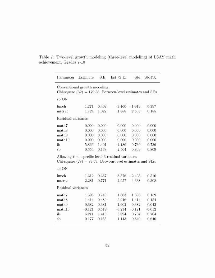
Table 7: Two-level growth modeling (three-level modeling) of LSAY mathachievement, Grades 7-10

Parameter Estimate S.E. Est./S.E. Std StdYX

Conventional growth modeling:Chi-square (32) = 179.58. Between-level estimates and SEs:

sb ON

lunch -1.271 0.402 -3.160 -1.919 -0.397mstrat 1.724 1.022 1.688 2.605 0.185

Residual variances

math7 0.000 0.000 0.000 0.000 0.000math8 0.000 0.000 0.000 0.000 0.000math9 0.000 0.000 0.000 0.000 0.000math10 0.000 0.000 0.000 0.000 0.000ib 5.866 1.401 4.186 0.736 0.736sb 0.354 0.138 2.564 0.809 0.809

Allowing time-specific level 3 residual variances:Chi-square (28) = 83.69. Between-level estimates and SEs:

sb ON

lunch -1.312 0.367 -3.576 -2.495 -0.516mstrat 2.281 0.771 2.957 4.338 0.308

Residual variances

math7 1.396 0.749 1.863 1.396 0.159math8 1.414 0.480 2.946 1.414 0.154math9 0.382 0.381 1.002 0.382 0.042math10 -0.121 0.518 -0.234 -0.121 -0.012ib 5.211 1.410 3.694 0.704 0.704sb 0.177 0.155 1.143 0.640 0.640

32

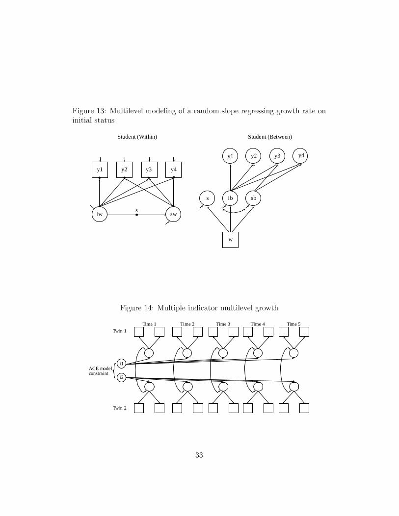
Figure 13: Multilevel modeling of a random slope regressing growth rate oninitial status

ib sb

y1 y2 y3 y4

w

s

y1 y2 y3 y4

iw sws

Student (Within) Student (Between)

Figure 14: Multiple indicator multilevel growth

Time 1 Time 2 Time 3 Time 4 Time 5Twin 1

Twin 2

i1

i2

ACE modelconstraint

33

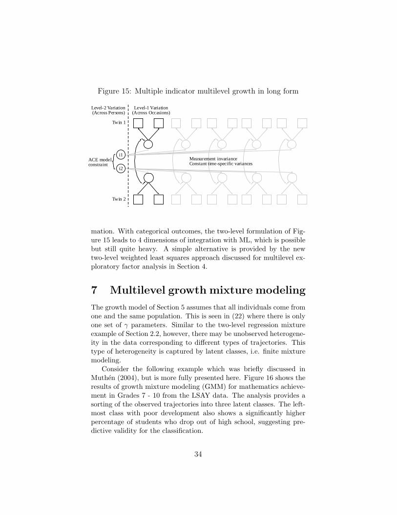
Figure 15: Multiple indicator multilevel growth in long form

Level-1 Variation(Across Occasions)

Twin 1

Twin 2

i1

i2

ACE modelconstraint

Level-2 Variation(Across Persons)

Measurement invarianceConstant time-specific variances

mation. With categorical outcomes, the two-level formulation of Fig-ure 15 leads to 4 dimensions of integration with ML, which is possiblebut still quite heavy. A simple alternative is provided by the newtwo-level weighted least squares approach discussed for multilevel ex-ploratory factor analysis in Section 4.

7 Multilevel growth mixture modeling

The growth model of Section 5 assumes that all individuals come fromone and the same population. This is seen in (22) where there is onlyone set of γ parameters. Similar to the two-level regression mixtureexample of Section 2.2, however, there may be unobserved heterogene-ity in the data corresponding to different types of trajectories. Thistype of heterogeneity is captured by latent classes, i.e. finite mixturemodeling.

Consider the following example which was briefly discussed inMuthen (2004), but is more fully presented here. Figure 16 shows theresults of growth mixture modeling (GMM) for mathematics achieve-ment in Grades 7 - 10 from the LSAY data. The analysis provides asorting of the observed trajectories into three latent classes. The left-most class with poor development also shows a significantly higherpercentage of students who drop out of high school, suggesting pre-dictive validity for the classification.

34

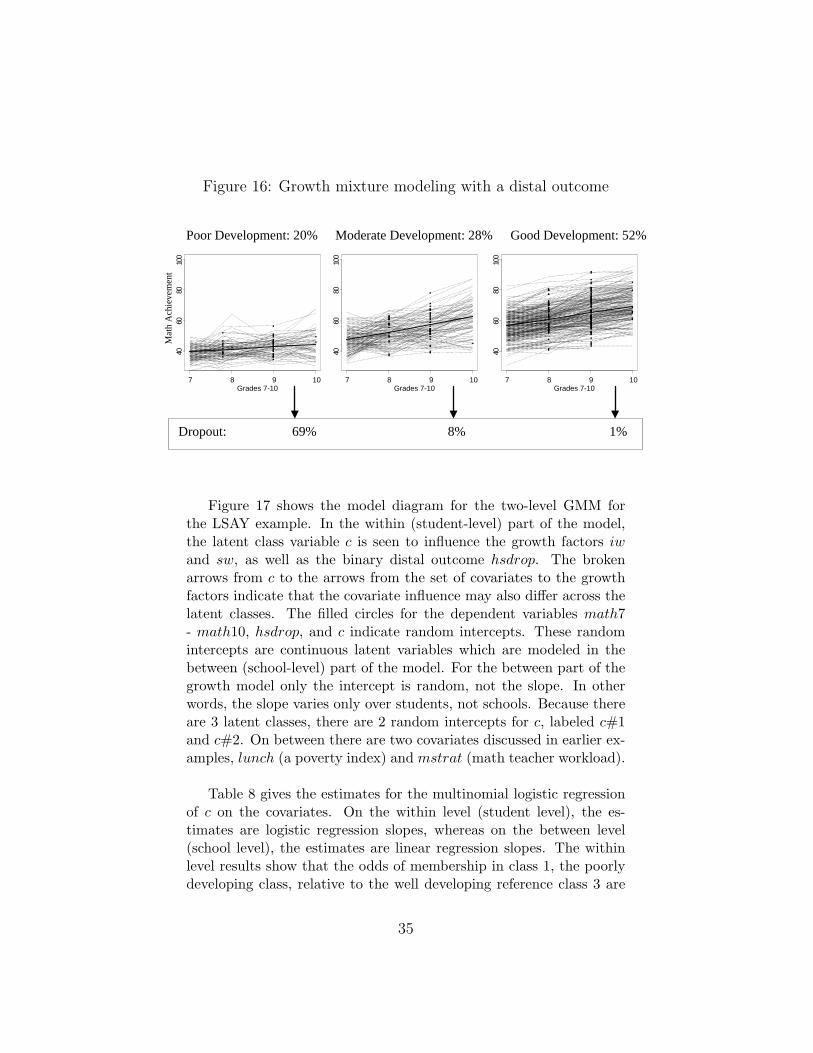
Figure 16: Growth mixture modeling with a distal outcome

Mat

h A

chie

vem

ent

7 8 9 10

4060

8010

0

Grades 7-107 8 9 10

4060

8010

0

Grades 7-107 8 9 10

4060

8010

0

Grades 7-10

Poor Development: 20% Moderate Development: 28% Good Development: 52%

Dropout: 69% 8% 1%

Figure 17 shows the model diagram for the two-level GMM forthe LSAY example. In the within (student-level) part of the model,the latent class variable c is seen to influence the growth factors iwand sw, as well as the binary distal outcome hsdrop. The brokenarrows from c to the arrows from the set of covariates to the growthfactors indicate that the covariate influence may also differ across thelatent classes. The filled circles for the dependent variables math7- math10, hsdrop, and c indicate random intercepts. These randomintercepts are continuous latent variables which are modeled in thebetween (school-level) part of the model. For the between part of thegrowth model only the intercept is random, not the slope. In otherwords, the slope varies only over students, not schools. Because thereare 3 latent classes, there are 2 random intercepts for c, labeled c#1and c#2. On between there are two covariates discussed in earlier ex-amples, lunch (a poverty index) and mstrat (math teacher workload).

Table 8 gives the estimates for the multinomial logistic regressionof c on the covariates. On the within level (student level), the es-timates are logistic regression slopes, whereas on the between level(school level), the estimates are linear regression slopes. The withinlevel results show that the odds of membership in class 1, the poorlydeveloping class, relative to the well developing reference class 3 are

35

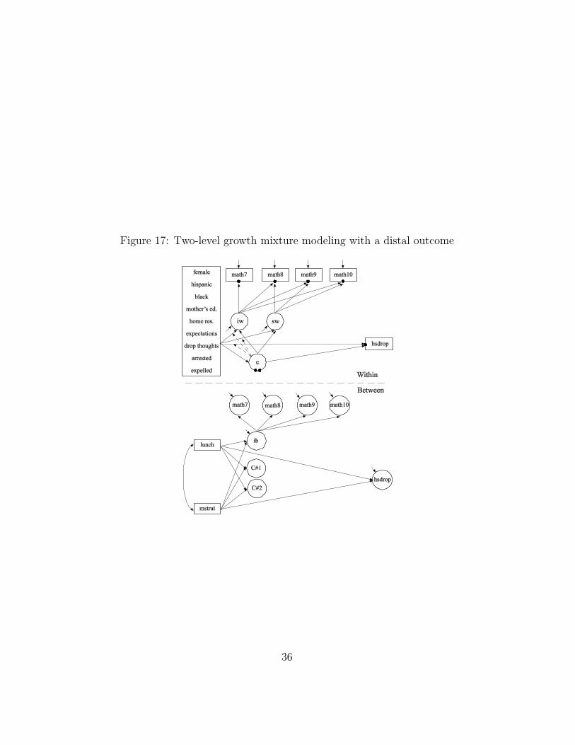
Figure 17: Two-level growth mixture modeling with a distal outcome

36

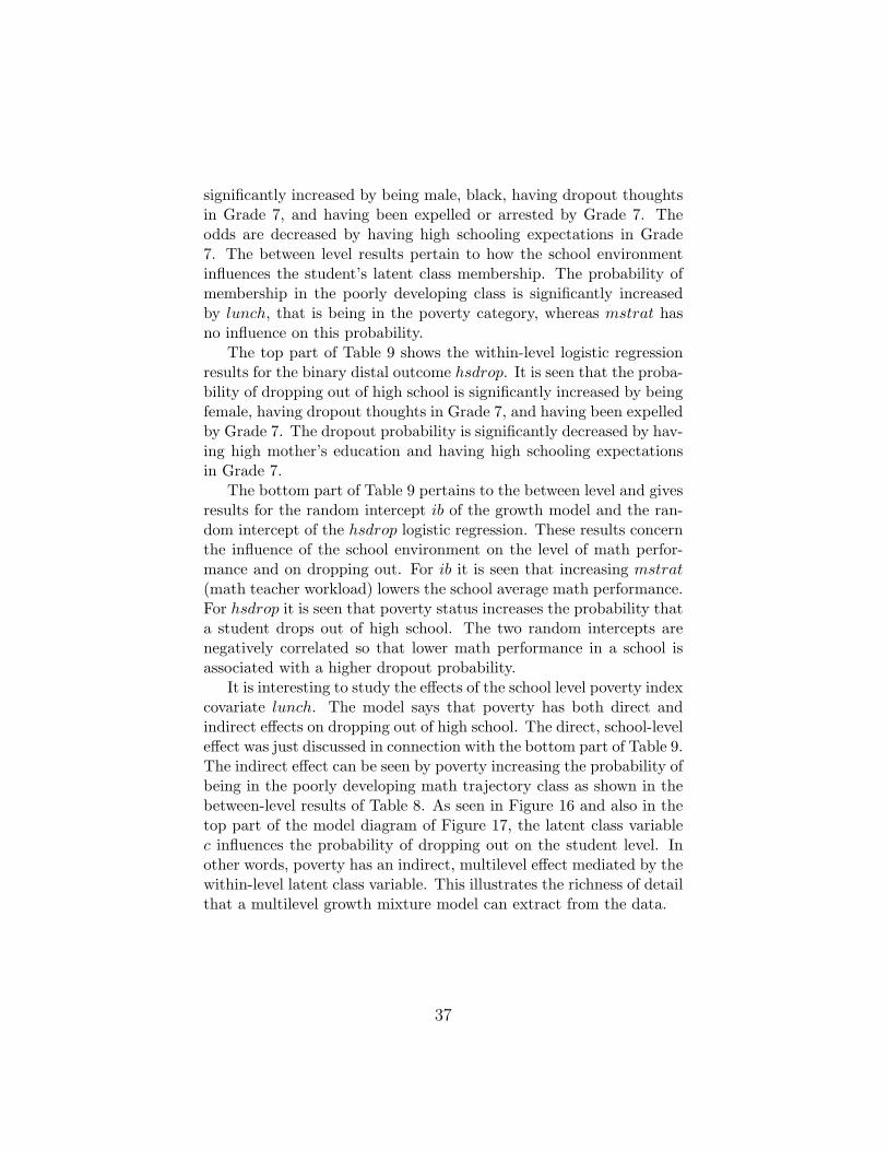
significantly increased by being male, black, having dropout thoughtsin Grade 7, and having been expelled or arrested by Grade 7. Theodds are decreased by having high schooling expectations in Grade7. The between level results pertain to how the school environmentinfluences the student’s latent class membership. The probability ofmembership in the poorly developing class is significantly increasedby lunch, that is being in the poverty category, whereas mstrat hasno influence on this probability.

The top part of Table 9 shows the within-level logistic regressionresults for the binary distal outcome hsdrop. It is seen that the proba-bility of dropping out of high school is significantly increased by beingfemale, having dropout thoughts in Grade 7, and having been expelledby Grade 7. The dropout probability is significantly decreased by hav-ing high mother’s education and having high schooling expectationsin Grade 7.

The bottom part of Table 9 pertains to the between level and givesresults for the random intercept ib of the growth model and the ran-dom intercept of the hsdrop logistic regression. These results concernthe influence of the school environment on the level of math perfor-mance and on dropping out. For ib it is seen that increasing mstrat(math teacher workload) lowers the school average math performance.For hsdrop it is seen that poverty status increases the probability thata student drops out of high school. The two random intercepts arenegatively correlated so that lower math performance in a school isassociated with a higher dropout probability.

It is interesting to study the effects of the school level poverty indexcovariate lunch. The model says that poverty has both direct andindirect effects on dropping out of high school. The direct, school-leveleffect was just discussed in connection with the bottom part of Table 9.The indirect effect can be seen by poverty increasing the probability ofbeing in the poorly developing math trajectory class as shown in thebetween-level results of Table 8. As seen in Figure 16 and also in thetop part of the model diagram of Figure 17, the latent class variablec influences the probability of dropping out on the student level. Inother words, poverty has an indirect, multilevel effect mediated by thewithin-level latent class variable. This illustrates the richness of detailthat a multilevel growth mixture model can extract from the data.

37

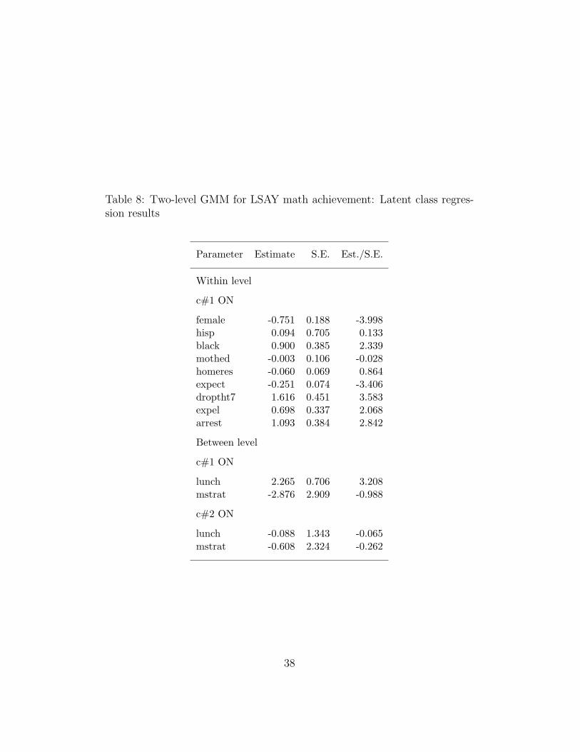
Table 8: Two-level GMM for LSAY math achievement: Latent class regres-sion results

Parameter Estimate S.E. Est./S.E.

Within level

c#1 ON

female -0.751 0.188 -3.998hisp 0.094 0.705 0.133black 0.900 0.385 2.339mothed -0.003 0.106 -0.028homeres -0.060 0.069 0.864expect -0.251 0.074 -3.406droptht7 1.616 0.451 3.583expel 0.698 0.337 2.068arrest 1.093 0.384 2.842

Between level

c#1 ON

lunch 2.265 0.706 3.208mstrat -2.876 2.909 -0.988

c#2 ON

lunch -0.088 1.343 -0.065mstrat -0.608 2.324 -0.262

38

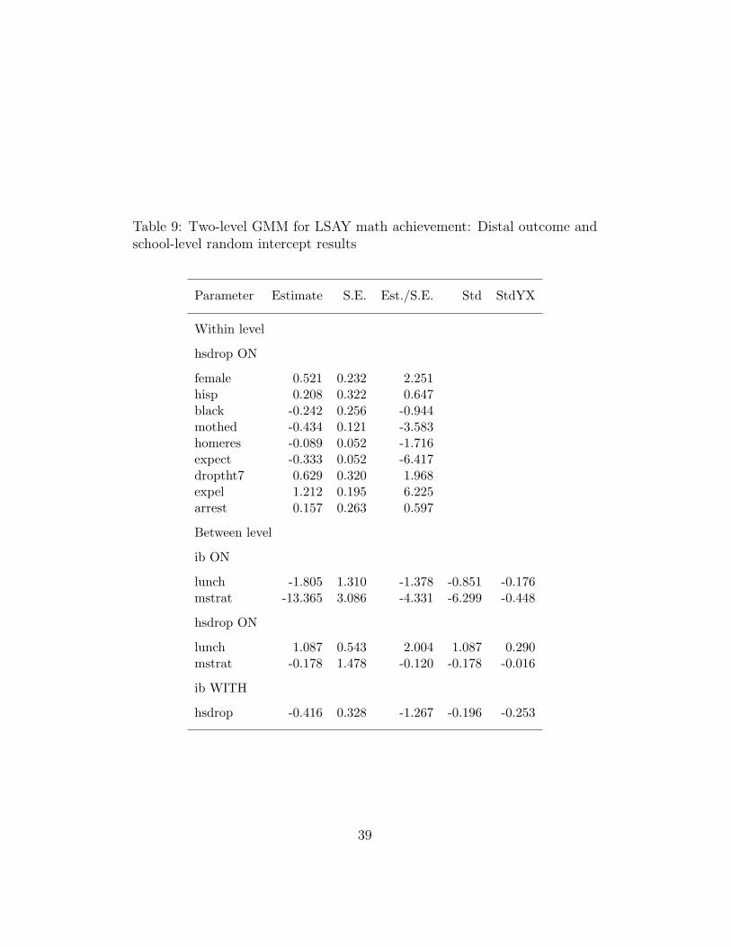
Table 9: Two-level GMM for LSAY math achievement: Distal outcome andschool-level random intercept results

Parameter Estimate S.E. Est./S.E. Std StdYX

Within level

hsdrop ON

female 0.521 0.232 2.251hisp 0.208 0.322 0.647black -0.242 0.256 -0.944mothed -0.434 0.121 -3.583homeres -0.089 0.052 -1.716expect -0.333 0.052 -6.417droptht7 0.629 0.320 1.968expel 1.212 0.195 6.225arrest 0.157 0.263 0.597

Between level

ib ON

lunch -1.805 1.310 -1.378 -0.851 -0.176mstrat -13.365 3.086 -4.331 -6.299 -0.448

hsdrop ON

lunch 1.087 0.543 2.004 1.087 0.290mstrat -0.178 1.478 -0.120 -0.178 -0.016

ib WITH

hsdrop -0.416 0.328 -1.267 -0.196 -0.253

39

8 Conclusions

This chapter has given an overview of latent variable techniques formultilevel modeling that are more general than those commonly de-scribed in text books. Most if not all of the models cannot be handledby conventional multilevel modeling or software. If space permitted,many more examples could have been given. For example, using com-binations of model types, one may formulate a two-part growth modelwith individuals nested within clusters, or a two-part growth mixturemodel. Several multilevel models such as latent class analysis, latenttransition analysis, and discrete- and continuous-time survival analy-sis can also be combined with the models discussed. All these modeltypes fit into the general latent variable modeling framework availablein the Mplus program.

40

References

[1] Asparouhov, T., Masyn, K. & Muthen, B. (2006). Continuous timesurvival in latent variable models. Proceedings of the Joint Statis-tical Meeting in Seattle, August 2006. ASA section on Biometrics,180-187.

[2] Asparouhov, T., & Muthen, B. (2006). Constructing covariates inmultilevel regression. Mplus Web Notes: No. 11.

[3] Asparouhov, T. & Muthen, B. (2007). Computationally efficientestimation of multilevel high-dimensional latent variable models.Proceedings of the 2007 JSM meeting in Salt Lake City, Utah, Sec-tion on Statistics in Epidemiology.

[4] Asparouhov, T. & Muthen, B. (2008). Exploratory structuralequation modeling. Forthcoming in Structural Equation Modeling.

[5] Bauer, Preacher & Gil (2006). Conceptualizing and testing randomindirect effects and moderated mediation in multilevel models: Newprocedures and recommendations. Psychological Methods, 11, 142-163.

[6] Little, R.J., & Rubin, D.B. (2002). Statistical analysis with missingdata. Second edition. New York: John Wiley & Sons.

[7] Ludtke, O., Marsh, H.W., Robitzsch, A., Trautwein, U., As-parouhov, T., & Muthen, B. (2008). The multilevel latent covariatemodel: A new, more reliable approach to group-level effects in con-textual studies. Psychological Methods, 13, 203-229.

[8] Muthen, B. (1989). Latent variable modeling in heterogeneouspopulations. Psychometrika, 54, 557-585.

[9] Muthen, B. (2004). Latent variable analysis: Growth mixturemodeling and related techniques for longitudinal data. In D. Ka-plan (ed.), Handbook of quantitative methodology for the socialsciences (pp. 345-368). Newbury Park, CA: Sage Publications.

[10] Muthen, B. & Asparouhov, T. (2008). Growth mixture modeling:Analysis with non-Gaussian random effects. In Fitzmaurice, G., Da-vidian, M., Verbeke, G. & Molenberghs, G. (eds.), LongitudinalData Analysis, pp. 143-165. Boca Raton: Chapman & Hall/CRCPress.

[11] Muthen, B. & Asparouhov, T. (2009). Multilevel regression mix-ture analysis. Forthcoming in Journal of the Royal Statistical Soci-ety, Series A.

41

[12] Muthen, L. & Muthen, B. (2008). Mplus User’s Guide. Los An-geles, CA: Muthen & Muthen.

[13] Olsen, M.K. & Schafer, J.L. (2001). A two-part random effectsmodel for semicontinuous longitudinal data. Journal of the Ameri-can Statistical Association, 96, 730-745.

[14] Raudenbush, S.W. & Bryk, A.S. (2002). Hierarchical linear mod-els: Applications and data analysis methods. Second edition. New-bury Park, CA: Sage Publications.

[15] Seltzer, M., Choi, K., Thum, Y.M. (2002). Examining relation-ships between where students start and how rapidly they progress:Implications for conducting analyses that help illuminate the distri-bution of achievement within schools. CSE Technical Report 560.CRESST, University of California, Los Angeles.

[16] Schmidt, W. H. (1969). Covariance structure analysis of the mul-tivariate random effects model. Unpublished doctoral dissertation,University of Chicago.

[17] Snijders, T. & Bosker, R. (1999). Multilevel analysis. An in-troduction to basic and advanced multilevel modeling. ThousandOakes, CA: Sage Publications.

42