Better Weather Forecasts Resulting from Improved Land ... · 13/01/2015 · Better Weather...
43
Stéphane Bélair Better Weather Forecasts Resulting from Better Weather Forecasts Resulting from Improved Land Surface Processes in Improved Land Surface Processes in EC's Numerical Prediction Systems EC's Numerical Prediction Systems GSFC, NASA, 13 January 2015 Meteorological Research Division Environment Canada
Transcript of Better Weather Forecasts Resulting from Improved Land ... · 13/01/2015 · Better Weather...

Stéphane Bélair
Better Weather Forecasts Resulting from Better Weather Forecasts Resulting from Improved Land Surface Processes in Improved Land Surface Processes in EC's Numerical Prediction SystemsEC's Numerical Prediction Systems
GSFC, NASA, 13 January 2015
Meteorological Research DivisionEnvironment Canada

Greater Emphasis on Surface Meteorology
Upper-air evaluation to compare Centers' performance
Different approach (more global) needed to determine true value of NWP systems
Emphasis on near-surface forecasts, felt by most NWP clients

Many Clients / Systems to Interface with
GridSpacing(km)
Forecast Length (days)
Sub-Monthly NWP SystemsAt Environment Canada 1
10
50
1 2 10
RDPSNorth Amer.
EnVar
GDPSGlobalEnVar
10km
GEPSGlobalEnKF
50km
REPSNorth Amer.Downscaling
15km
2.5kmHRDPSCanada
Downscaling
25km25
250mExperimentalLocal / UrbanDownscaling

EC's Effort to Improve Land Surface
Characteristics and properties
Modeling – representation of processes
Data assimilation
Coupling with atmosphere

The Surface Processor - Characteristics
(Vanh Souvanlasy)
GenPhysX /UrbanX
PreX
GEM orGEM-Surf
DATABASES
GTOPO30GMTED2010SRTM-DEM-v4ASTER-DEMCDED2012USGS-GLCCMODIS-MCD12Q1CCRSGlobCover2.3LCC2000-VCanVec-9.0OSMNLCD2006Census-StatCan2006FAOCANSISBNU Soil DatasetJPL Soil TypeUSDA STATSGOHWSD3D GlobVegNHD, NHN
Orographic parametersWater fraction
Vegetation fractionsUrban parametersWater fractionSoil textureDrainage Density
MODIS ALBEDO CLIM.MODIS NDVI CLIM.BIOME-BGC CLIM.
LEAF AREA INDEXVEG. FRACTIONSVEG. PARAMETERSALBEDOsROOT-ZONE DEPTHSANDCLAYURBAN PARAMETERS
IN
OUT

Example: Global, 15 km, surface roughness
Yin
Yang
(Bernard Bilodeau)

Example: Regional, 2.5 km, Veg. Height
(m)
Simard et al. (2011) – JPLFrom GLAS aboard ICESat
Used for Z0 (local only), no orographic component

Impact on Near-Surface Winds
Reglam vs B3 (z0 from LUT)20 summer cases (00 UTC)Reglam vs B35 (z0 from JPL)
10-m wind speed STDEs
(Manon Faucher)
Pan Canadian 2.5-km system
ControlControl
Previous exp.
With new roughness

Example: Local, 250 m, land cover
LAI (m2m-2)
LAKEONTARIO
GREATER TORONTO AREA
Light grey: pavement fractionDark brown: building fraction

Example: Local, 250 m, urban
Building fraction
(Vanh Souvanlasy)

Example: Local, 250 m, urban
Pavementfraction
(Vanh Souvanlasy)
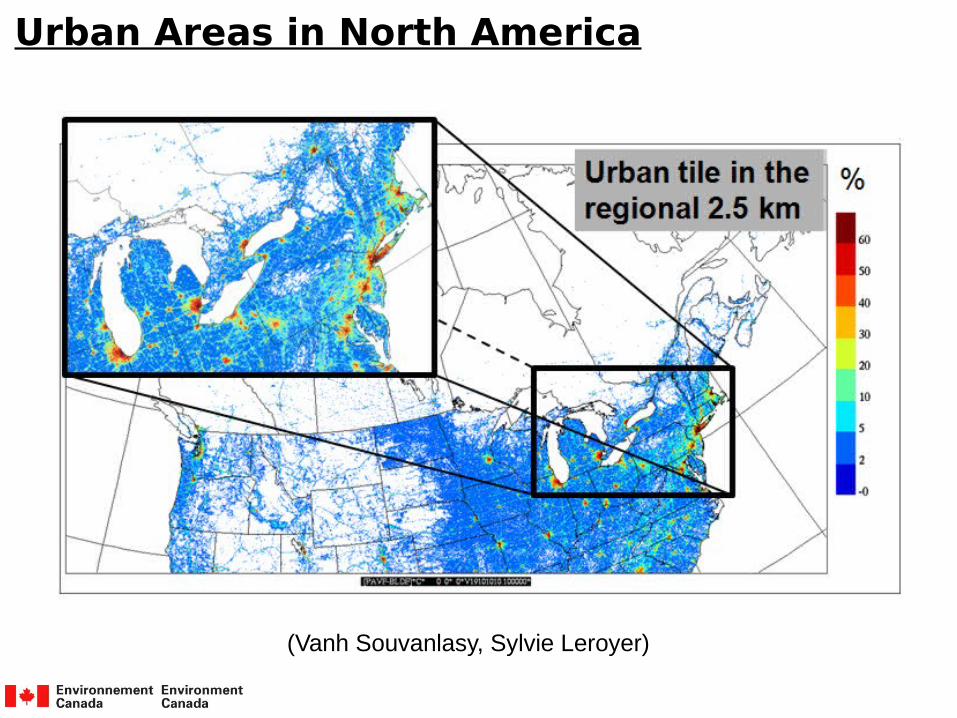
Urban Areas in North America
(Vanh Souvanlasy, Sylvie Leroyer)

Land Surface Models
Sea ice
Soil and vegetation
Glaciers
Water
Urban
Natural Land
Water
Urban
Glaciers
Sea ice
Snow
ISBA, SVS, CLASS
Simple scheme with constant surface temperature (NEMO for 3D lakes + 1D lake model)
TEB
Force-restore scheme (with snow), module from CLASS
3-layer model with snow on top (LIM2 or CICE)
Simple schemes over glaciers and sea ice; one layer model in ISBA and SVS, slightly more complex in TEB and CLASS

The Soil, Vegetation, and Snow Scheme
Multiple energy and water budgets (new subgrid-scale tiling)
Multi-layer model for soil moisture
New snow pack under the vegetation
Root density function depending on vegetation type
Changes to vegetation thermal coefficient, albedo, and emissivity
Stomatal resistance from photosynthesis scheme
Not changed: still a single canopy layer scheme
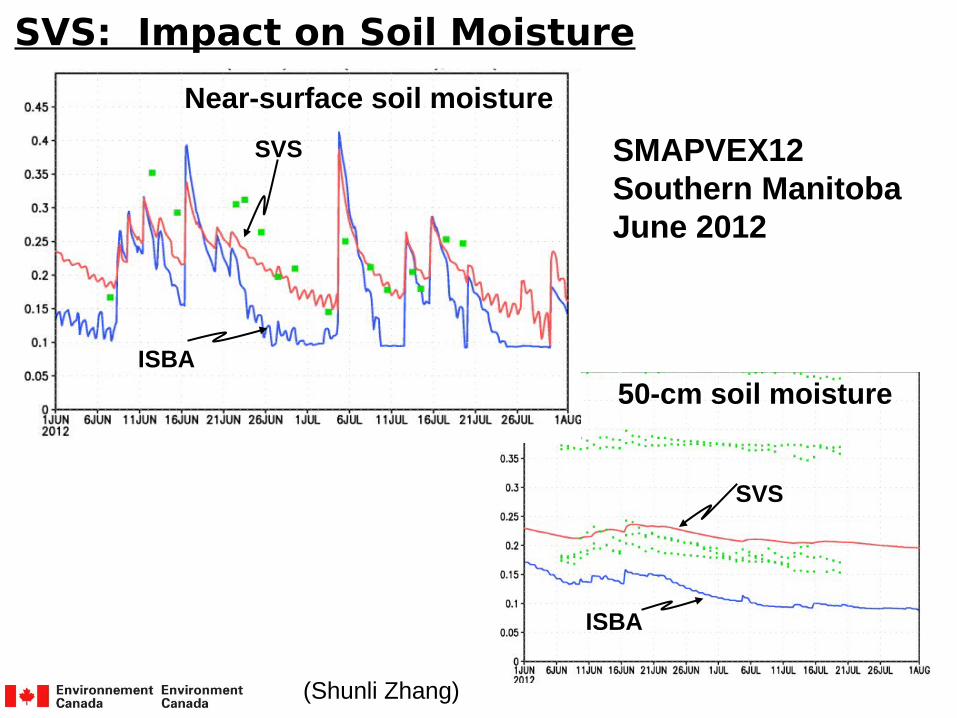
SVS: Impact on Soil Moisture
SVS
ISBA
SVS
ISBA
Near-surface soil moisture
50-cm soil moisture
SMAPVEX12Southern ManitobaJune 2012
(Shunli Zhang)

SVS: Impact on L-Band Forward Modeling
ISBACORRELATION MEAN: 0.44
SVSCORRELATION MEAN: 0.46
Horizontal Polarization : 40o Incidence AngleMay – September 2012
(Shunli Zhang, Marco Carrera)

EC's Land Data Assimilation Effort
LANDMODEL(SPS)
OBS
ASSIMILATIONEnKF + EnOI
xb
y
EnKFxa = xb+ K { y – H(xb) }
K = BHT ( HBHT+R)-1
with
CaLDASIN OUT
Ancillary land surface data
Atmospheric forcing
Observations
Surface Temperature
Soil moisture
Snow depth or SWE
Vegetation*
Screen-level (T, Td)Surface stations snow depthL-band passive (SMOS, SMAP)MW passive (AMSR-E)*Optical / IR (MODIS, VIIRS)Combined products (GlobSnow)
T, q, U, V, Pr, SW, LW
Orography, vegetation, soils, water fraction, ...
Analyses of…
*) not done yet…

First Implementations of CaLDAS
Screen-level air temperature and dew point temperature
EnKF Soil moisture and surface temperature
Surface obs of snow depth
EnOI Snow water equivalent
OBS Method Control variables
Regional (Canada + part of USA), 2.5 kmGlobal, Yin-Yang grid, 25 km
Both systems implemented in Fall 2014 at MSC-Operations

CaLDAS: Impact on HRDPS (2.5 km)
RMSE, Td_2m20 summer casesCanada
With CaLDAS
Without CaLDAS
(Manon Faucher)

CaLDAS: Impact on RDPS (10 km)
RMSE, TT_2m20 summer casesUSA
With CaLDAS
Without CaLDAS
(Jean-Francois Caron)

CaLDAS: Impact on GDPS (25 km)
Upper-air evaluationAgainst radiosondesSouthern HemisphereJune-July-AugustAbout 100 cases5-day forecasts
(Bernard Bilodeau)

CaLDAS: Impact on GEPS (Ensemble)
Continuous Rank Probability Score (CRPS)
Reliability component of the CRPS
Over North America
2-m temperature
CTRL
With CaLDAS
CTRL
With CaLDAS(Normand Gagnon)

Assimilation of L-Band Data in CaLDAS
SMOS NRT-light L-band Tbs (40 km, multi-angles)
QA/QC: exclusive alias-free zone, simple tests
Rescaling of Tbs based on CDF matching
Tb obs. error chosen as 5 K (homogeneous)
EnKF: 24 members, 10 km analyses, wg and w2
EnKF: 3h frequency, CMEM forward model
Tested in synthethic mode and over SMAPVEX12

Impact of L-Band Data on Soil Moisture
AAFC SAGES mean
(5, 20 and 50 cm).
Mean of sampled fields
(6 cm)
m3 m-3
m3 m-3
SMAPVEX12 - Manitoba
CaLDAS-SMOS-10km
Open loop
CaLDAS-SMOS-10km
Open loop
(Marco Carrera)

Towards a More Complete CaLDAS
Starting point: CaLDAS-screen 2.5km (OP)
Addition of the SMOS component (combination with screen-level obs, simultaneous or sequential)
Addition of the SVS surface scheme for the first guess
To be tested first in regional 10-km mode (NAM)
To be extended afterward to Canada 2.5-km (first) and to global 15 km (second)

Ready for SMAP... (Passive at Least...)
Current monitoring of SMOS observationSame apparatus will be used for SMAPTest with data as soon as possible
http://meteocentre.com/plus/

Traditional Land-Atmosphere Coupling
Height of lowest atmosphericlevel
Vertical resolutionnear the surface
Exchangecoefficients

EC R&D on Land – Atmosphere Coupling
Lower atmospheric levels near the surface (as close as 1.5m for thermodynamic level)
Changes to the nature of the land-atmosphere interactions with atmospheric levels intersecting with vegetation and urban canopies.
Two-way coupling: low-res atmospheric model with high-res surface system

Figure 1 in Bernier and Belair, 2012, J. Appl. Meteorol.
Increased Vertical Resolution near Surface

Figure 3 in Bernier and Belair, 2012, J. Appl. Meteorol.
15 winter cases, and 15 summer cases
Impact on Screen-Level Variables

Figure 4 in Bernier and Belair, 2012, J. Appl. Meteorol.
15 winter cases, and 15 summer cases
00Z
12Z
Impact on Near-Surface Profiles
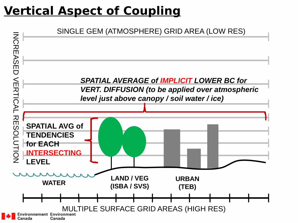
LAND / VEG(ISBA / SVS)
URBAN(TEB)
WATER
SINGLE GEM (ATMOSPHERE) GRID AREA (LOW RES)
MULTIPLE SURFACE GRID AREAS (HIGH RES)
INC
RE
AS
ED
VE
RT
ICA
L RE
SO
LUT
ION
SPATIAL AVERAGE of IMPLICIT LOWER BC for VERT. DIFFUSION (to be applied over atmospheric level just above canopy / soil water / ice)
SPATIAL AVG of TENDENCIES for EACH INTERSECTING LEVEL
Vertical Aspect of Coupling

CaM-TEB (Canadian Multilayer version of TEB)
Several model levels intersect the buildings.
Variable building heights exist within a grid cell.
(Husain et al. 2013)
Coupling Urban Canopy with Atmosphere

LAND / VEG(ISBA / SVS)
URBAN(TEB)
WATER
SINGLE GEM (ATMOSPHERE) GRID AREA (LOW RES)
MULTIPLE SURFACE GRID AREAS (HIGH RES)
∂ θ∂ t
=1ρ
∂∂ z ( ρ KT
∂ θ∂ z )=−
1ρ
∂∂ z
ρ w ' θ '______
−(w ' θ '______ )
S=αθ+βθ θNK atm
+
(w ' θ '______
)S=CT u¿ [θS
+−f S θNK atm
+ ] α θ=−CT u¿ θS+
βθ=−CT u¿ f S
SPATIAL AVERAGE OF IMPLICIT LOWER BC FOR VERT. DIFFUSION
Spatially averaged
Horizontal Aspect of Coupling

Towards 2-Way Coupling
(Rochoux et al, 2015, submitted)
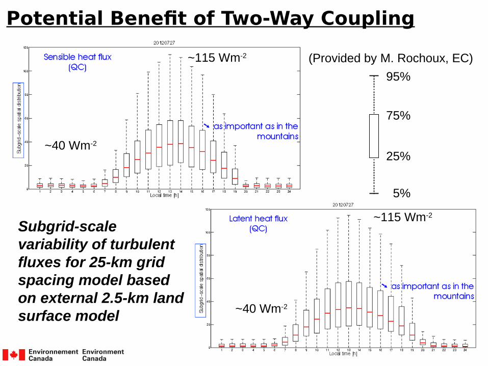
Subgrid-scale variability of turbulent fluxes for 25-km grid spacing model based on external 2.5-km land surface model
95%
5%
25%
75%
~115 Wm-2
~115 Wm-2
(Provided by M. Rochoux, EC)
~40 Wm-2
~40 Wm-2
Potential Benefit of Two-Way Coupling

Final Words
An effort much greater than originally expected when this new phase started a decade ago...
All aspects important
Comments and recommendations are welcome!

The end... backup slides (urban stuff)

The Town and Energy Balance Scheme(Masson, 2000)
Street canyonconcept :Drag, radiation budgets
Input:Urban fabric (material layers, depths)Morphology (aspect ratio, roughness)
Output :Surface temperatures, Energy budgets,
T, q, wind at pedestrian level
Multiple reflections,trappingabsorption

TEB: Urban Heat Islands
(oC)
(Leroyer et al., 2011)
• Radiative Surface Temperature (°C) July 6th 2008 (10:54 LST)
Urban offline model (100-m grid spacing)

TEB: Urban Heat Islands
(oC)
• Radiative Surface Temperature (°C) July 6th 2008 (10:54 LST)
Urban offline model (100-m grid spacing)
MODIS, 1km
(Leroyer et al., 2011)

Tokyo Case: Urban Areas
Radar / Raingauge Analysis (JMA) GEM - 250m
19-h Forecast(with TEB)
(Courtesy of N. Seino, JMA/MRI)
(Lubos Spacek)

Tokyo Case: Impact of TEB
19-h ForecastValid at 1600 JST
26 Aug. 2011
CONTROL RUN – with URBAN
Without URBAN (no TEB)
(Lubos Spacek)