Best Practices for Assessing Health and Determining ... · i Final Report Best Practices for...

i

Final Report

BestPracticesforAssessingCulvertHealthandDetermining

AppropriateRehabilitationMethods

A Research Project in Support of Operational Requirements

for the South Carolina Department of Transportation

Principal Investigators

Kalyan R. Piratla and Weichiang Pang

Student Investigators

He Jin and Michael Stoner

Glenn Department of Civil Engineering,

Clemson University

November 2016

ii

Technical Report Documentation Page 1. Report No.

FHWA‐SC‐17‐01

2. Government Accession No.

3. Recipient's Catalog No.

4. Title and Subtitle

Best Practices for Assessing Culvert Health and Determining Appropriate Rehabilitation Methods

5. Report Date

February 2017 6. Performing Organization Code

7. Author(s)

Kalyan R. Piratla and Weichiang Pang 8. Performing Organization Report No.

9. Performing Organization Name and Address

Glenn Department of Civil Engineering Clemson University 109 Lowry Hall Clemson, SC 29634

10. Work Unit No. (TRAIS) 11. Contract or Grant No.

SPR 718

12. Sponsoring Agency Name and Address

South Carolina Department of Transportation Office of Materials and Research 1406 Shop Road Columbia, SC 29201

13. Type of Report and Period Covered

Final Report 14. Sponsoring Agency Code

15. Supplementary Notes

16. Abstract Due to the invisibility of buried culverts from the surface, they often get ignored until a problem such as road settlement or flooding arises. Many of the existing culverts in the US are in a deteriorated state having reached the end of their useful design life. Consequently, there have been several reported cases of culvert failures that caused the collapse of roads which pose a significant safety risk to motorists. The overarching goal of this research project is to provide technical guidance to the South Carolina Department of Transportation (SCDOT) in effectively managing their culvert infrastructure. Four specific objectives identified are: (1) develop guidance on the latest culvert inspection techniques for use by SCDOT; (2) develop a deterioration model to predict the future condition of culverts; (3) develop a risk‐based renewal prioritization model for deteriorating culverts; and (4) develop guidance for selecting optimal renewal methods given the culvert material, size, and user preferences. The findings of this study provide preliminary guidance for the management of culvert infrastructure by maintenance departments at state and district levels. Specifically, the models developed for deterioration prediction, risk‐based prioritization, and renewal selection would aid in effective short‐term and long‐term planning of culvert infrastructure maintenance.

17. Key Word

Culvert Inspection, Culvert Rehabilitation, Culvert Deterioration

18. Distribution Statement

No restrictions

19. Security Classif. (of this report)

Unclassified 20. Security Classif. (of this page)

Unclassified 21. No. of Pages

22. Price

Form DOT F 1700.7 (8-72) Reproduction of completed page authorized

iii

Acknowledgments

The research team acknowledges the funding offered by the South Carolina Department of

Transportation and the Federal Highway Administration in support of this research project. We

extend our sincere thanks to the project Steering and Implementation Committee which includes

the following members:

Jim Johannemann –Chairman

Kevin Harrington

Dusty Turner

Perry Crocker

Ken Johnson, FHWA

The authors would like to thank the civil engineering graduate students He Jin and Michael Stoner

who worked on this project. Their tireless efforts were instrumental in the execution of this

research project. This project resulted in one PhD dissertation and one Masters’ thesis written by

He Jin and Michael Stoner, respectively. The authors would also like to thank Dr. John Matthews for

his helpful inputs and feedback.

The authors would like to acknowledge the support of the SCDOT Office of Materials and Research

staff, especially Mr. Terry Swygert and Ms. Meredith Casteel. Finally, the authors would like to

thank all the state departments of transportation that participated in the survey conducted as part

of this research study.

iv

Disclaimer

The contents of this report reflect the views of the authors who are responsible for the facts and

the accuracy of the presented data. The contents do not reflect the official views of SCDOT or

FHWA. This report does not constitute a standard, specification, or regulation.

v

Executive Summary

Millions of culverts exist in the United States. Several DOTs are responsible for more number of culverts than bridge structures within their jurisdiction. Due to the invisibility of buried culverts from the surface, they often get ignored until a problem such as road settlement or flooding arises. Many of the existing culverts in the US are in a deteriorated state having reached the end of their useful design life. Consequently, there have been several reported cases of culvert failures in the US that caused the collapse of roads which pose a significant safety risk to motorists. In addition to the safety risk, culvert failures could be prohibitively expensive due to emergency repair costs, traffic congestion, and detours. Yet, transportation agencies lack effective culvert management practices when compared to bridges and pavements.

Although SCDOT has a well‐devised rating methodology for inspecting culvert structures, there is lack of guidance on predicting culvert conditions into the future, prioritizing culvert structures for repair and also choosing an appropriate repair method. The overarching goal of this research project is to provide technical guidance to SCDOT in effectively managing their culvert infrastructure. Effective management entails the use of economical and reliable procedures for early identification and repair of culverts in despair before they inflict catastrophic failures on the transportation infrastructure. Four specific objectives identified are:

1. Develop guidance on the latest culvert inspection techniques for use by SCDOT. 2. Develop a deterioration model to predict the future condition of culverts. 3. Develop a risk‐based renewal prioritization model for deteriorating culverts. 4. Develop guidance for selecting optimal renewal methods for a given culvert material, size and

other user preferences.

The results from this study would inform guidelines for effective management of SCDOT’s culvert structures by maintenance departments at state‐ and district‐level. Specific benefits include: (a) SCDOT can leverage the preliminary guidance presented in this report on culvert inspection techniques to more effectively choose condition assessment techniques when there is a need for a detailed inspection of culvert structures far and beyond the torch‐enabled manual inspection from the inlet or the outlet; (b) SCDOT can leverage the deterioration modeling effort and the associated statistical analysis presented in this report to keep track of the important parameters that have been found to be influencing the culvert condition, and also predict the condition of the culverts into the future for effective inspection and capital improvement planning; (c) SCDOT can employ the risk‐based prioritization model presented in this report to more effectively shortlist a set of culverts that need immediate attention; (d) SCDOT can use the developed Culvert Renewal Selection Tool (CREST) both at district‐ and state‐ level to identify an optimal set of potential culvert renewal techniques depending on its material, size, prevailing defect, and defect severity. While the benefits are manifold, it may take some effort to seamlessly integrate the guidelines and tools developed in this study into the operational procedures of SCDOT.

vi

Table of Contents

Acknowledgments ....................................................................................................................... iii

Disclaimer .................................................................................................................................... iv

Executive Summary ...................................................................................................................... v

Table of Contents ........................................................................................................................ vi

List of Figures............................................................................................................................. viii

List of Tables ................................................................................................................................. x

List of Acronyms ........................................................................................................................ xiii

Commonly Used Terminology for Culverts ................................................................................ xv

1. INTRODUCTION .......................................................................................................................... 1

1.1 Introduction and Problem Statement ................................................................................... 1

1.2 Research Objectives .............................................................................................................. 2

1.3 Benefits of This Research ...................................................................................................... 2

1.4 Organization of the Report ................................................................................................... 3

2. CULVERT CONDITION ASSESSMENT GUIDANCE ......................................................................... 4

2.1 Culvert Inspection Techniques: An Overview ....................................................................... 5

2.2 Evaluation of Inspection Techniques and Mapping of Defects ............................................. 9

2.4 Chapter Summary ................................................................................................................ 10

3. CULVERT DETERIORATION MODELING ..................................................................................... 11

3.1 SCDOT Culvert Inventory Analysis ....................................................................................... 12

3.2 Composite Inspection Ratings ............................................................................................. 21

3.3 Deterioration Modeling Inputs ........................................................................................... 22

3.4 Deterioration Modeling Effort ............................................................................................ 31

3.4.1 Logistic Regression Analysis ............................................................................................. 31

3.4.2 Artificial Neural Networks ................................................................................................ 34

3.5 Primary Outcomes: Model Discussions, Comparisons, and Conclusions ........................... 38

3.6 Model Conclusions .............................................................................................................. 46

3.6 Chapter Summary ................................................................................................................ 49

vii

4. RISK‐BASED CULVERT RENEWAL PRIORITIZATION ................................................................... 50

4.1 SCDOT Culvert Inventory Analysis and Defect Categorization............................................ 50

4.2 Survey of Other States ........................................................................................................ 50

4.3 Risk‐based Culvert Renewal Prioritization Model ............................................................... 54

4.4 Model Demonstration and Outcomes ................................................................................ 54

4.5 Chapter Summary........................................................................................................... 59

5. CULVERT RENEWAL GUIDANCE ................................................................................................ 61

5.1 Culvert Renewal Techniques: Alternatives ......................................................................... 62

5.2 Evaluation of Culvert Renewal Techniques ......................................................................... 67

5.3 Culvert Renewal Selection Guidance .................................................................................. 72

5.4 Demonstration .................................................................................................................... 73

5.4.1 Results and Discussion ..................................................................................................... 73

5.4 Validation of the CREST Model ......................................................................................... 100

5.5 Limitations ......................................................................................................................... 106

5.6 Chapter Summary .............................................................................................................. 106

6. CONCLUSIONS AND RECOMMENDATIONS ............................................................................. 108

6.1 Major Outcomes and Limitations of the Research ........................................................... 108

6.2 Benefits to SCDOT ............................................................................................................. 110

Appendix A: Culvert Deterioration Age Information .................................................................. 111

Appendix B: Copy of the Risk Assessment Survey ...................................................................... 117

Appendix C: Failure Risk Analysis Results ................................................................................... 119

Appendix D: Case Studies for Validation .................................................................................... 123

7. REFERENCES ............................................................................................................................ 127

viii

List of Figures

Figure 1. Illustration of inspection methods: (a) CCTV , (b) Sonar scanning, (c) Laser profiling, (d)

Ultrasonic inspection, (e) Infrared thermography, and (f) GPR ..................................................... 7

Figure 2. Common Defects Observed in Culverts ........................................................................... 9

Figure 3. Distribution of the Variables Addressed in the Culvert Inspection Guide ..................... 14

Figure 4. Conceptual Reasoning for Separate Output Models ..................................................... 17

Figure 5. Temperature distribution across South Carolina ........................................................... 24

Figure 6. Precipitation distribution across South Carolina ........................................................... 25

Figure 7. pH distribution across South Carolina ........................................................................... 26

Figure 8. Distribution of South Carolina Land Cover (NLCD) ........................................................ 27

Figure 9. Relationship between Observed Culverts and Average Number of Inputs ................... 37

Figure 10. Trend Types for Input Coefficients of Logistic Regression Models .............................. 39

Figure 11. Distribution of Effect of Primary Input Variables ........................................................ 40

Figure 12. Demonstration of Negative Coefficients and Positive Impact..................................... 42

Figure 13. CMP Composite Score DOT Estimate 1 with Error Term ............................................. 45

Figure 14. Spatial Bias Potential in Models with Fewer Input Culverts ........................................ 46

Figure 15. Model Overview and Usage ......................................................................................... 49

Figure 16. Route type distribution for RCP culverts measured by length .................................... 56

Figure 17. Route type distribution for CMP culverts measured by length ................................... 57

Figure 18. Failure Risk Analysis of RCP Culverts: Risk vs. Length .................................................. 58

Figure 19. Failure Risk Analysis of CMP Culverts: Risk vs. Length ................................................ 59

Figure 20. Illustrations of culvert renewal methods: (a) Open‐cut, (b) Internal grouting, (c)

Robotic grouting, (d) Internal shotcreting, (e) Robotic shotcreting, (f) Slip‐lining, (g) CIPP, (h)

Fold and form lining, (i) Spiral wound lining, (j) Centrifugally‐cast .............................................. 66

Figure 21. Percentage preference of OC for various application scenarios for RCP culverts ...... 78

Figure 22. Percentage preference of SL for various application scenarios for RCP culverts ........ 79

Figure 23. Percentage preference of CIPP (semi‐structural) for various application scenarios for

RCP culverts .................................................................................................................................. 80

ix

Figure 24. Percentage preference of CIPP (full‐structural) for various application scenarios for

RCP culverts .................................................................................................................................. 80

Figure 25. Percentage preference of SWL (semi‐structural) for various application scenarios for

RCP culverts .................................................................................................................................. 81

Figure 26. Percentage preference of SWL (full‐structural) for various application scenarios for

RCP culverts .................................................................................................................................. 82

Figure 27. Percentage preference of PB for various application scenarios for RCP culverts ....... 82

Figure 28. Percentage preference of OC for various application scenarios for CMP culverts ..... 93

Figure 29. Percentage preference of IS for various application scenarios for CMP culverts ....... 94

Figure 30. Percentage preference of SL for various application scenarios for CMP culverts ...... 95

Figure 31. Percentage preference of CIPP (semi‐structural) for various application scenarios for

CMP culverts ................................................................................................................................. 96

Figure 32. Percentage preference of CIPP (full‐structural) for various application scenarios for

CMP culverts ................................................................................................................................. 97

Figure 33. Percentage preference of SWL (semi‐structural) for various application scenarios for

CMP culverts ................................................................................................................................. 98

Figure 34. Percentage preference of SWL (full‐structural) for various application scenarios for

CMP culverts ................................................................................................................................. 99

Figure 35. Percentage preference of CCCP for various application scenarios for CMP culverts 100

Figure 36. Distribution of Ages for Specified Culverts ................................................................ 112

Figure 37. CMP Average Composite Score ................................................................................. 115

Figure 38. CMP DOT Estimate 1 Composite Score ...................................................................... 115

Figure 39. CMP DOT Estimate 2 Composite Score ...................................................................... 116

Figure 40. Barrel Failure Risk Assessment Survey ...................................................................... 118

x

List of Tables

Table 1. Advantages and limitations of culvert inspection methods ............................................. 8

Table 2. Mapping of defects to inspection techniques ................................................................ 10

Table 3. Inventory Information provided by SCDOT Culvert Inspection Guide ............................ 13

Table 4. Assessment Information provided by SCDOT Culvert Inspection Guide ........................ 14

Table 5. Distribution of Culvert Types in SCDOT Database .......................................................... 18

Table 6. Average rating for each culvert type and each output category .................................... 19

Table 7. Breakdown of SCDOT Culvert Database ......................................................................... 20

Table 8. Results of Survey to State DOTs ...................................................................................... 21

Table 9. Defect Matching Between DOT Survey and Culvert Inspection Guide ........................... 21

Table 10. Relative Importance of Output Ratings ........................................................................ 22

Table 11. Dummy Variable Creation ............................................................................................. 23

Table 12. ALCCS Classifications used to describe the NLCD Maps ............................................... 27

Table 13. South Carolina Runoff Coefficients Used in Hydraulic Design ...................................... 28

Table 14. ALCCS Pixel Data and Corresponding Runoff Coefficient from SCDOT ......................... 29

Table 15. Possible Input Variables and Assumed Importance ...................................................... 30

Table 16. Combinations of Input Variables Tested ....................................................................... 31

Table 17. Area under Curve Results (Logistic Regression) ............................................................ 33

Table 18. Area Under Curve Results (Artificial Neural Network) .................................................. 35

Table 19. Cost Emphasis Matrix .................................................................................................... 36

Table 20. Coefficient of Determination (R2) ................................................................................. 43

Table 21. Standard Deviation for Each Model Type and Composite Weight ............................... 45

Table 22. Distribution of Culvert Ratings ...................................................................................... 47

Table 23. Breakdown of Better Model ......................................................................................... 48

Table 24. Criteria used by SCDOT for the assessment of culverts ................................................ 50

Table 25. Defects in RCP and CMP culverts that may lead to the barrel failure .......................... 51

Table 26. Definitions of defects that may be seen on a culvert barrel ........................................ 52

Table 27. Threshold defect severity .............................................................................................. 52

Table 28. Quantitative conversion scale used for the culvert failure risk assessment survey ..... 53

xi

Table 29. Criticality of various barrel defects ............................................................................... 54

Table 30. Defect mapping for RCP culverts .................................................................................. 55

Table 31. Defect mapping for CMP culverts ................................................................................. 55

Table 32. Failure consequence scores .......................................................................................... 56

Table 33. Significant advantages and limitations of culvert renewal methods ............................ 65

Table 34. Performance Classes for the Selected Decision Criteria ............................................... 67

Table 35. Comparative evaluation of semi‐structural renewal techniques for <36” dia. culverts

....................................................................................................................................................... 69

Table 36. Evaluation of semi‐structural renewal techniques for 36”‐60”dia. culverts ................ 69

Table 37. Evaluation of semi‐structural renewal techniques for 60”‐120” dia. culverts ............. 70

Table 38. Evaluation of full‐structural renewal techniques for <36” dia. culverts ....................... 70

Table 39. Evaluation of full‐structural renewal techniques for 36”‐60” dia. culverts .................. 71

Table 40. Evaluation of full‐structural renewal techniques for 60”‐120” dia. culverts ................ 71

Table 41. Mapping of RCP application scenarios to renewal types and techniques for <36” dia.

culverts .......................................................................................................................................... 74

Table 42. Mapping of RCP application scenarios to renewal types and techniques for 36”‐60”

dia. culverts ................................................................................................................................... 75


dia. culverts ................................................................................................................................... 76

Table 44. Range of criteria weightings for semi‐ and full‐ structural culvert renewal techniques

for RCP culverts ............................................................................................................................. 77


....................................................................................................................................................... 84

Table 46. Comparative evaluation of semi‐structural renewal techniques for 36”‐60” dia.

culverts .......................................................................................................................................... 84

Table 47. Comparative evaluation of semi‐structural renewal techniques for 60”‐120” dia.

culverts .......................................................................................................................................... 84

Table 48. Comparative evaluation of full‐structural culvert renewal techniques for <36” dia.

culverts .......................................................................................................................................... 85

xii

Table 49. Comparative evaluation of full‐structural culvert renewal techniques for 36”‐60” dia.

culverts .......................................................................................................................................... 85

Table 50. Comparative evaluation of full‐structural culvert renewal techniques for 60”‐120” dia.

culverts .......................................................................................................................................... 85

Table 51. Mapping of CMP application scenarios to renewal types and techniques for <36” dia.

culverts .......................................................................................................................................... 87

Table 52. Mapping of CMP application scenarios to renewal types and techniques for 36”‐60”

dia. culverts ................................................................................................................................... 88

Table 53. Mapping of CMP application scenarios to renewal types and techniques for 60”‐120”

dia. culverts ................................................................................................................................... 89

Table 54. Range of criteria weightings for semi‐structural culvert renewal techniques ............. 90

Table 55. Range of criteria weightings for full‐structural culvert renewal techniques of sizes <36

inches diameter ............................................................................................................................ 91

Table 56. Range of criteria weightings for full‐structural culvert renewal techniques of sizes 36”‐

120” diameter ............................................................................................................................... 92

Table 57. Selected culvert defects and case studies for validation ............................................ 103

Table 58. Validation of findings for RCP applications ................................................................. 104

Table 59. Validation of findings for CMP applications ................................................................ 105

Table 60. Distribution of Culvert Ratings Compared to Overall Database ................................. 112

Table 61. Comparison of Models with and without Age ............................................................ 113

Table 62. Comparison of Models with and without Age ............................................................ 114

Table 63. Coefficient of Determination (R2) ............................................................................... 114

Table 64. RCP Culverts with Failure Risk Values Greater than 0.3 ............................................. 120

Table 65. CMP Culverts with Failure Risk Values Greater than 0.1 ............................................ 122

Table 66. Practical Case studies for RCP Applications ................................................................ 124

Table 67. Practical case studies for CMP applications (1) .......................................................... 125

Table 68. Practical case studies for CMP applications (2) .......................................................... 126

xiii

List of Acronyms

CMP – Corrugated metal pipe

RCP – Reinforced concrete pipe

HDPE – High density polyethylene

CAP – Corrugated aluminum pipe

PVC – Polyvinyl chloride

PE – Polyethylene

CREST – Culvert renewal selection tool

MDA – Multiple discriminant analysis

MLR – Multinomial logistic regression

ANN – Artificial neural network

NOAA – National oceanic and atmospheric administration

USGS – United States Geological Survey

NLCD – National land cover database

ALCCS – Anderson land cover classification system

ROC – Received operating characteristic

AHP – Analytical hierarchy process

C – Criticality score

FC – Consequence score

R – Failure risk

S – Overall selection score

NS – Non‐structural renewal

SS – Semi‐structural renewal

FS – Full structural renewal

PRV – Practice‐based reflective validation

VS – Validation score

MCDA – Multi‐criteria decision analysis

CCTV – Closed‐circuit television

GPR – Ground penetration radar

IT – Infrared thermography

C – Crack

ID – Invert deterioration

xiv

JM – Joint misalignment

JI – Joint inflow and exfiltration

CR – Corrosion

SD – Shape distortion

CIPP – Cured‐in‐place‐pipe

OC – Open cut method

IG – Internal grouting through human entry

RG – Robotic grouting

IS – Internal shotcreting through human entry

RS – Robotic shotcreting

SL – Sliplining

CCCP – Centrifugally‐case concrete pipe

FFL – Fold and form lining

SWL – Spiral wound lining

PB – Pipe bursting

xv

Commonly Used Terminology for Culverts

Barrel: The pipe or box section that facilitates the water flow under the roadway

Inlet: The entrance side of culvert flow

Outlet: The exit side of culvert flow

End Section: A concrete or metal structure placed at the end of a culvert to enhance hydraulic efficiency

Invert: The inside of the culvert’s bottom cross section

Crown: The inside of the top portion of a culvert

End treatment: Improvements to inlet or outlet geometry to maximize culvert flow capacity

Beveled End: End section where the top of the barrel is closer to the embankment than the bottom

Flared End: End section that flares out horizontally beyond the barrel of the culvert

Flat End: End section which is perpendicular to the line of the barrel

Apron: A horizontal structure attached at the inlet or outlet of the culvert to reduce erosion and

enhance hydraulic efficiency

Headwall: A structure placed at the inlet or outlet of a culvert to protect the embankment slopes and

prevent undercutting

Sedimentation: Soils and other materials that settle out of suspension and build up on the bottom of a

culvert

Piping (or Bedding voids): Water flowing along the outside of the culvert which over time erodes the soil

around or underneath the culvert barrel

Scour: Depletion of the culvert’s outlet channel due to erosive velocities

In/Exfiltration: The inflow or leakage through joint and other structural issues in a culvert

1

1. INTRODUCTION

1.1 Introduction and Problem Statement

Culverts are pipes that are typically located under roadways and embankments for the passage of water. They are designed to support the super‐imposed earth and live loads from passenger vehicle and trucks as well as the internal hydraulic loading from water flow. Culverts are differentiated from bridges based on their span length; smaller span bridges are usually referred as culverts. Millions of culverts exist in the United States. Some are managed by state DOTs and others by local governments and US Forestry Service. Several DOTs are responsible for more number of culverts than bridge structures within their jurisdiction (NCHRP, 2002). DOTs usually require that bridges and pavements are frequently inspected to ensure their safe operational condition. Due to the invisibility of buried culverts from the surface, they often get ignored until a problem such as road settlement or flooding arises. Many of the existing culverts in the US are in a deteriorated state having reached the end of their useful design life (Yang and Allouche, 2009). Consequently, there have been several reported cases of culvert failures in the US that caused the collapse of roads which pose a significant safety risk to motorists (Perrin Jr. and Jhaveri, 2004). In addition to the safety risk, culvert failures could be prohibitively expensive due to emergency repair costs, traffic congestion and detours. Yet, transportation agencies lack effective culvert management practices when compared to bridges and pavements (Najafi and Bhattachar, 2011).

South Carolina Department of Transportation (SCDOT) is responsible for the systematic planning, construction, maintenance, and operation of the fourth largest (over 42,000 miles) state highway system in the U.S. (SCFOR, 2014). Underneath those roads are tens of thousands of culverts that were installed over 50 years ago. A majority of SCDOT’s culverts are made of reinforced concrete pipe (RCP), corrugated metal pipe (CMP) and high density polyethylene (HDPE) materials. Traditionally, there has been less attention paid to culverts, especially to those that are less than 20 feet in span length, resulting in the lack of systematic inspection procedures. Consequently, there is little information available on the condition of SCDOT’s culvert infrastructure and it poses a risk to the public and state transportation infrastructure. Regular inspection of culverts in a proactive manner will aid SCDOT in prioritizing their repair (i.e. maintenance, rehabilitation, or replacement), and optimizing the use of limited financial resources available.

SCDOT has initiated a culvert inspection program in 2011, and launched an iPad application for easy and efficient collection of inventory and condition data in the field. A condition rating system was developed by SCDOT to record culvert condition data. The condition inspection is primarily done by external non‐intrusive human observations of culvert’s inlet, outlet, and barrel using flashlights and binoculars. Several categories of possible concern for inlets, outlets and barrels were identified as parameters that will be rated by field inspectors based on clearly‐defined objective guidelines. This program, currently in its initial phase, has focused on open‐ended storm drainage structures 36” and greater in width. The long‐term goal of this program is to conduct frequent culvert inspection to identify and prioritize most critical culvert

2

structures that need to be repaired soon. SCDOT is currently in its initial phase of implementing the culvert inspection program through collecting the first round of inventory and condition data of large diameter culverts.

While SCDOT has a well‐devised rating methodology, the condition assessment is permitted to less‐sophisticated human observation skills. It is difficult to accurately gauge the condition of a barrel from the outside of the culvert by a naked eye, especially in the case of long culverts. Consequently, there is a need for better assessment techniques for collecting more accurate condition data. Accurate condition data will lead to better predictions of future culvert condition and subsequent prioritization for rehabilitation. The current culvert inspection manual doesn’t provide guidance on how to prioritize culverts for repair based on the developed inspection and rating procedures. Additionally, it also doesn’t provide any guidance for selecting an appropriate repair method. This research study has been sponsored to address these pressing needs of SCDOT. The proposed research approach includes extensive literature review, risk‐based prioritization modeling, probabilistic deterioration prediction, survey of other DOTs, and development of decision‐trees.

1.2 Research Objectives

The overarching goal of this research project is to provide technical guidance to SCDOT in effectively managing their culvert infrastructure. Effective management entails the use of economical and reliable procedures for early identification and repair of culverts in despair before they inflict catastrophic failures on the transportation infrastructure. Four specific objectives identified are:

1. Develop guidance on culvert condition assessment techniques. 2. Develop a risk‐based model for prioritizing culvert rehabilitation based on the condition

rating data recorded by SCDOT. 3. Develop a deterioration model to predict the future condition of culverts in order to

optimally spend limited resources available on inspecting and repairing only those culverts that are critical and closer to failing.

4. Develop a decision‐making tool for selecting an economical and most effective culvert repair method based on condition rating and other culvert characteristics such as age, material, diameter, and etc.

1.3 Benefits of This Research

The results from this study produced broad guidelines for management of SCDOT’s culvert structures by maintenance departments at state‐ and district‐level. Specific benefits include: (a) SCDOT can leverage the preliminary guidance presented in this report on culvert inspection techniques to more effectively choose condition assessment techniques when there is a need for deeper investigation of culvert structures far and beyond the torch‐enabled manual inspection from the inlet or the outlet; (b) SCDOT can leverage the deterioration modeling effort and the associated statistical analysis presented in this report to keep track of the important parameters that have found to be influencing the culvert condition, and also predict

3

the condition of the culverts into the future for effective inspection and capital improvement planning; (c) SCDOT can employ the risk‐based prioritization model presented in this report to more effectively shortlist a set of culverts that need immediate attention; (d) SCDOT can use the developed Culvert Renewal Selection Tool (CREST) both at district‐ and state‐ level to identify an optimal set of potential culvert renewal techniques depending on material, size, prevailing defect, and expected defect severity. While the benefits are manifold, it may take some effort to seamlessly integrate the guidelines and tools developed in this study into the operational procedures of SCDOT.

1.4 Organization of the Report

This report is organized into six chapters. Chapter 2 presents guidance on culvert inspection techniques. Chapter 3 describes the culvert deterioration model that is developed in this study and discusses its merits and limitations. Chapter 4 presents the failure risk‐based renewal prioritization methodology for culvert infrastructure and demonstrates it using the preliminary culvert assessment data available in the SCDOT’s latest culvert inventory database. Chapter 5 describes various culvert renewal techniques while highlighting their special advantages and limitations, and also describes and demonstrates the Culvert Renewal Selection Tool (CREST) that is developed in this study. Chapter 6 summarizes the findings of this study, highlights its limitations and benefits.

4

2. CULVERT CONDITION ASSESSMENT GUIDANCE

Culvert failures could be prohibitively expensive due to emergency repair costs, unplanned traffic detours and the resulting congestion. Many culverts in the United States are deteriorated causing increased number of failures and subsequent collapses of the roads they are buried under. While the deterioration trend is primarily attributed to the prolonged usage beyond the intended design life, inadequate investment on timely maintenance and rehabilitation programs has expectedly aggravated the deterioration. A primary component of any culvert rehabilitation program is the condition assessment that reveals the accurate condition of the culvert and its estimated capacity to continue serving. Despite the availability of several non‐destructive condition assessment techniques, they are not often employed by culvert asset owners primarily due to cost and partly to lack of guidance. Several assessment techniques, which have a great potential for providing accurate quantitative condition assessment for better service life predictions, are described in this chapter with their advantages and limitations highlighted.

There are several published reports on culvert assessment frameworks (NCHRP, 2002; ODOT, 2003; FHWA, 2010). For example, the Federal Highway Administration’s (FHWA) Manual for Culvert Assessment and Decision Making Procedures provided guidelines for inspecting and rating the condition of culverts (FHWA, 2010). A majority of the past inspection and rating procedures are based on visual observations from the end (inlet or outlet) of the culvert aided by flash lights and mirrors. A majority of state departments of transportation (DOTs) developed their own inspection and condition rating procedures that also rely heavily on visual inspection from the ends of culverts. A few DOTs started using video cameras (i.e. CCTV) to inspect the culvert interiors.

Yang and Allouche (2009) thoroughly evaluated several non‐destructive technologies (NDT) to establish their suitability in assessing culvert condition based on their ability to detect particular defect types. Selvakumar et al. (2014) evaluated the technical performance and cost of five state‐of‐the‐art condition assessment techniques for sewer collection systems and compared them with the conventional CCTV technique. Culverts are non‐pressurized systems similar to gravity sewer pipelines and therefore condition assessment techniques evaluated in Selvakumar et al. (2014) would be technically suitable to them. The evaluated techniques are zoom camera, electro‐scanning, digital scanning, laser scanning and sonar scanning. The results revealed that: (a) digital scanning, zoom camera, CCTV, and laser scanning accurately assessed the pipe condition above the water line, whereas the sonar technique performed well below the water line, (b) electro‐scanning revealed leakage‐related defects all along the pipe circumference, and (c) total costs for the multi‐sensor (digital, laser, and sonar) inspection were found to be $14.71 per meter of pipeline inspected as compared to $10.31 per meter for electro‐scanning, $3.46 per meter for zoom camera, and about $10.13 per meter for CCTV (Selvakumar et al., 2014).

Although a few previous studies explored the suitability of various condition assessment techniques, there is a need for further investigation to produce guidance on their effective selection based on their advantages, limitations, and other specific considerations. This chapter

5

provides preliminary guidance on the state‐of‐the‐art pipeline inspection techniques that may be suitable for culverts. Specifically, the following techniques will be described: closed‐circuit television (CCTV), sonar scanning, laser profiling, ultrasonic inspection, infrared thermography, and ground penetrating radar (GPR) techniques. Drainage culverts are usually filled with significant amount of debris which may prevent the usage of any of these techniques in an economical manner. There is also limited evidence that suggests these sophisticated techniques are commonly employed for culvert inspection; they are however commonly employed for force main sewer, gravity sewer, and water pipeline inspection applications. Nevertheless, it is technically possible to employ these techniques for culvert inspection.

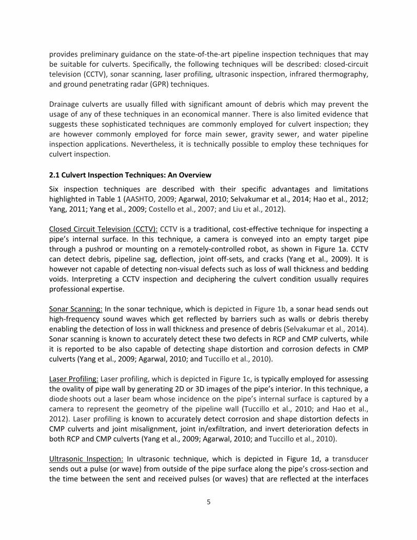
2.1 Culvert Inspection Techniques: An Overview

Six inspection techniques are described with their specific advantages and limitations highlighted in Table 1 (AASHTO, 2009; Agarwal, 2010; Selvakumar et al., 2014; Hao et al., 2012; Yang, 2011; Yang et al., 2009; Costello et al., 2007; and Liu et al., 2012). Closed Circuit Television (CCTV): CCTV is a traditional, cost‐effective technique for inspecting a pipe’s internal surface. In this technique, a camera is conveyed into an empty target pipe through a pushrod or mounting on a remotely‐controlled robot, as shown in Figure 1a. CCTV

can detect debris, pipeline sag, deflection, joint off‐sets, and cracks (Yang et al., 2009). It is however not capable of detecting non‐visual defects such as loss of wall thickness and bedding voids. Interpreting a CCTV inspection and deciphering the culvert condition usually requires professional expertise. Sonar Scanning: In the sonar technique, which is depicted in Figure 1b, a sonar head sends out high‐frequency sound waves which get reflected by barriers such as walls or debris thereby enabling the detection of loss in wall thickness and presence of debris (Selvakumar et al., 2014). Sonar scanning is known to accurately detect these two defects in RCP and CMP culverts, while it is reported to be also capable of detecting shape distortion and corrosion defects in CMP culverts (Yang et al., 2009; Agarwal, 2010; and Tuccillo et al., 2010). Laser Profiling: Laser profiling, which is depicted in Figure 1c, is typically employed for assessing the ovality of pipe wall by generating 2D or 3D images of the pipe’s interior. In this technique, a diode shoots out a laser beam whose incidence on the pipe’s internal surface is captured by a camera to represent the geometry of the pipeline wall (Tuccillo et al., 2010; and Hao et al., 2012). Laser profiling is known to accurately detect corrosion and shape distortion defects in CMP culverts and joint misalignment, joint in/exfiltration, and invert deterioration defects in both RCP and CMP culverts (Yang et al., 2009; Agarwal, 2010; and Tuccillo et al., 2010). Ultrasonic Inspection: In ultrasonic technique, which is depicted in Figure 1d, a transducer sends out a pulse (or wave) from outside of the pipe surface along the pipe’s cross‐section and the time between the sent and received pulses (or waves) that are reflected at the interfaces

6

between materials of varying properties is monitored for defect detection. The interfaces of varying properties are caused by structural or corrosion defects (Agarwal, 2010; and Yang et al., 2009). Ultrasonic technique is popularly known to detect corrosion in CMP culverts and wall thinning in both RCP and CMP culverts (Yang et al., 2009; Agarwal, 2010; and Tuccillo et al., 2010). Infrared Thermography: Infrared thermography technique, which is depicted in Figure 1e, is typically employed for detecting pipe bedding issues. In this technique, thermal sensors detect subsurface defects by measuring the temperature emitted from different subsurface materials and from subsequently analyzing the temperature distributions based on the colors of the images (Agarwal, 2010; and Yang et al., 2009). Infrared thermography is known to detect bedding voids in both RCP and CMP culverts (Yang et al., 2009; and Tuccillo et al., 2010). Ground Penetrating Radar (GPR): GPR technique, which is depicted in Figure 1f, is typically employed for detecting bedding issues, similar to infrared thermography. In this technique, high frequency electromagnetic waves are transmitted into the ground through an antenna from the ground level and the reflected electromagnetic waves from various underground materials are collected and analyzed. GPR technique works by measuring the time lag between transmitted and reflected waves which corresponds to the depth or the distance of the reflecting material (Agarwal, 2010; and Yang et al., 2009). GPR is popularly known to identify bedding voids in both RCP and CMP culverts (Yang et al., 2009 and Tuccillo et al., 2010).

7

Figure 1. Illustration of inspection methods: (a) CCTV , (b) Sonar scanning, (c) Laser profiling, (d) Ultrasonic inspection, (e) Infrared thermography, and (f) GPR

8

Table 1. Advantages and limitations of culvert inspection methods

Technique Advantages Limitations

CCTV

Provides direct illuminated image of pipe defects

Can be viewed in different angles

Real‐time assessment

Only provides qualitative information

Pre‐cleaning of the culvert is required

Only useful above the waterline

Sonar scanning

Can measure loss in wall thickness

Works in live flow conditions

Complements laser profiling by providing additional information

Needs specially‐trained work force

Works in air or under water but not at the same time

Cannot be used for inspection of brick pipes

Laser profiling

Produces a 3D model for a better QA/QC

Real‐time recording and analysis

Complements CCTV by providing additional information

Only useful above the waterline

Pre‐cleaning and drying of the culvert is required

Needs skilled data analysts

Ultrasonic scanning

Produces results in 2D or 3D formats

Can detect invisible defects within the culvert wall

Non‐invasive

Pre‐cleaning of the culvert is required (internal ultrasonic)

Dewatering is required (internal ultrasonic)

Need excavation for access to pipe surface

Infrared thermography

Non‐invasive

Typically economical

Highly productive

Wind speed and ground cover influence results

Affected by soil properties

Need to clearly differentiate color shades for accurate results

GPR Produces immediate results

Available for internal and above‐ground inspection

Cleaning of the pipe is not required

Difficult to move the equipment in uneven ground

Needs skilled operators

Difficult in ground water conditions

9

2.2 Evaluation of Inspection Techniques and Mapping of Defects

Commonly observed defects in culverts that are of concern include crack, invert deterioration, joint misalignment, joint infiltration or exfiltration, corrosion, shape distortion, debris, loss of wall thickness, and bedding voids. Several of these defects are depicted in Figure 2. These defects are appropriately mapped with culvert materials they usually manifest in and also with the six inspection techniques based on their respective abilities to detect these defects (Yang et al., 2009; Agarwal, 2010; and Tuccillo et al., 2010), as shown in Table 2.

Figure 2. Common Defects Observed in Culverts

10

Table 2. Mapping of defects to inspection techniques

Defects Materials Techniques

Debris RCP, CMP, HDPE

CCTV

Sonar

Laser

Crack RCP, HDPE CCTV

Sonar

Invert deterioration RCP, CMP

CCTV

Laser

Sonar

Joint misalignment RCP, CMP, HDPE CCTV

Laser

Joint in/exfiltration RCP, CMP CCTV

Laser

Wall thinning RCP, CMP

Sonar

Ultrasonic

Laser

Bedding voids RCP, CMP, HDPE IT

GPR*

Corrosion CMP

CCTV

Laser

Sonar

Ultrasonic

Shape distortion CMP Laser

Sonar *unreliable

2.4 Chapter Summary

It is vital that culvert asset owners employ economical and reliable inspection techniques to be aware of the prevailing condition of their culvert infrastructure and subsequently prepare for future needs in terms of technical, financial, and human resources. This chapter described six pipeline inspection techniques that may be suitable for culvert inspection when it is cleared of any pre‐existing debris.

11

3. CULVERT DETERIORATION MODELING

Culverts can be defined as pipes which are typically located under a roadway and help to direct the flow of water. Culverts differ from bridges in that they are smaller and often hidden below the roadway. Because culverts are often concealed and can be difficult to access, their condition can be hard to determine through traditional inspection techniques. In South Carolina alone, there are tens of thousands of culverts that were installed over 50 years ago and are in varying states of deterioration. With such a large infrastructure of culverts, it is important to be able to prioritize the repair and rehabilitation efforts. The failure mechanisms of culverts can vary extensively, and the condition of a culvert can be the combination of many different criteria. In addition, there are many factors that affect the condition of a culvert that include both physical and environmental characteristics. The behavior of a culvert is largely affected by its material type. In South Carolina, six primary types of culverts are used: reinforced concrete pipe (RCP), corrugated metal pipe (CMP), corrugated aluminum pipe (CAP), high density polyethylene pipe (HDPE), masonry pipe, and mixed type or other type culverts. Of these six types of culverts, RCP culverts are by far the most common in the state of South Carolina. The combination of these characteristics and their relationship with the condition of the culvert is complex in nature.

Previous researchers have used Markov models to predict deterioration of culverts, as well as multiple discriminant analysis (MDA) to predict the structural deterioration of culverts. This study will focus primarily on creating multinomial logistic regression (MLR) and artificial neural network (ANN) models that can be used to predict the condition of a culvert without on‐site investigations or assessments. These models will serve to predict a variety of output characteristics for each culvert as well as provide different models for each culvert type. The output predicted by the model will be combined using a weighted average. These weights can be determined by the model’s user or by previous data collected from various state Departments of Transportation and will give the user an idea of the overall health of a culvert as well as the variability that exists within each model. The goal of these models is to give an estimate of a culvert’s state of deterioration using physical and environmental characteristics that allow the user to prioritize those culverts that need further assessment and ultimately repair and replacement.

The primary objective of the deterioration modeling task was to create and verify a model that could be used to predict the condition of culverts in South Carolina. This model was based on a database of historical data that was used to pair a culvert’s physical and environmental characteristics with the condition assessment of the culvert. Two different model types were used to predict the probability that a culvert will require repair or comprehensive inspection in an attempt to maximize the efficiency of the repair and assessment techniques. The multinomial logistic regression (MLR) and artificial neural network (ANN) models attempted to predict the condition all six culvert types and all required assessment variables defined by the South Carolina Department of Transportation Culvert Inspection Guide.

The probabilistic model was not a deterioration model, because a time‐dependent variable associated with each culvert was absent from the database of culvert information. Using other

12

physical and environmental parameters in combination with physical characteristics associated with each culvert, the model was used to identify the effects of these parameters and determine a culvert overall condition. The accurate mapping and assignment of the site specific parameters not included in the database of information was also an important objective in this study. In addition to creating the two models, regression techniques were used to post‐process the output produced by these models in an effort to correct for any present bias and quantify the variability that exists in the population of culverts in South Carolina. These models also depended on several factors including the number of neurons in each layer, the training algorithms used to create the network, and the combinations of input variables. These variants were manipulated to give the most accurate neural network model. The final models will allow the user to determine the output rating of any of the criteria used in the SCDOT Field Inventory and Inspection Guidelines as well as determine a composite score for each of the culverts. Using regression analysis, a final composite score would be calculated and the standard deviation would be presented. These efforts were made in order to accurately identify the culverts in South Carolina in need of assessment or repair without performing any physical testing or on‐site investigation.

3.1 SCDOT Culvert Inventory Analysis

The information that was provided by the South Carolina Department of Transportation followed the format of the SCDOT Pipe & Culvert Field Inventory and Inspection Guidelines 2011. This document outlined the information that was required during field assessments as well as the scale for which these assessment categories are to be measured. The database of information was split into two sections, culvert inventory and culvert assessment. The culvert inventory included information shown in Table 5.1. These characteristics largely describe the physical properties of the culverts in South Carolina. Important characteristics from the inventory database include Culvert ID and Number, Culvert Type, culvert dimensions, and latitude and longitude coordinates.

The culvert assessment database contained all the information in regards to an assessment of the culverts listed in the culvert inventory. The categories provided in the assessment database are shown in Table 3.

13

Table 3. Inventory Information provided by SCDOT Culvert Inspection Guide

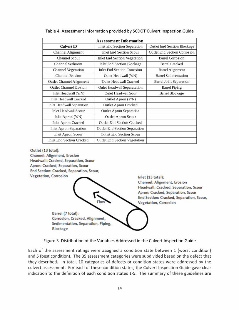
The information from the assessment criteria outlined in the SCDOT Culvert Inspection Guidelines 2011 was meant to address three main areas of each culvert, the inlet, the outlet, and the culvert barrel (Table 4 and Figure 3). In total, 35 assessment categories were ranked in order to give a condition of the culvert.

District Liner Diameter

County Liner Width

Route Type Liner Height

Route Num Liner Notes

AUX Inlet Pipe End Type

Beg MP Inlet End Treatment

End MP Inlet Apron Type

Culvert ID Outlet Pipe End Type

Culvert Num Outlet End Treatment

Num Barrells Outlet Apron Type

Culvert Type Date Inventoried

Culvert Shape Inventoried By

Diameter Date Modified

Width Modified By

Height Lat

Length Long

Liner Type Geo Accuracy

Inventory Information

14

Table 4. Assessment Information provided by SCDOT Culvert Inspection Guide

Figure 3. Distribution of the Variables Addressed in the Culvert Inspection Guide

Each of the assessment ratings were assigned a condition state between 1 (worst condition) and 5 (best condition). The 35 assessment categories were subdivided based on the defect that they described. In total, 10 categories of defects or condition states were addressed by the culvert assessment. For each of these condition states, the Culvert Inspection Guide gave clear indication to the definition of each condition states 1‐5. The summary of these guidelines are

Culvert ID Inlet End Section Separation Outlet End Section Blockage

Channel Alignment Inlet End Section Scour Outlet End Section Corrosion

Channel Scour Inlet End Section Vegetation Barrel Corrosion

Channel Sediment Inlet End Section Blockage Barrel Cracked

Channel Vegetation Inlet End Section Corrosion Barrel Alignment

Channel Erosion Oulet Headwall (Y/N) Barrel Sedimentation

Outlet Channel Alignment Oulet Headwall Cracked Barrel Joint Separation

Outlet Channel Erosion Oulet Headwall Separatation Barrel Piping

Inlet Headwall (Y/N) Oulet Headwall Sour Barrel Blockage

Inlet Headwall Cracked Outlet Apron (Y/N)

Inlet Headwall Separation Outlet Apron Cracked

Inlet Headwall Scour Outlet Apron Separation

Inlet Apron (Y/N) Outlet Apron Scour

Inlet Apron Cracked Outlet End Section Cracked

Inlet Apron Separation Outlet End Section Separation

Inlet Apron Scour Outlet End Section Scour

Inlet End Section Cracked Outlet End Section Vegetation

Assessment Information

15

shown below. The total number of assessment values that are related to the category are shown in parenthesis.

CRACKING (7)

1. Cracks greater than 1”, exposed rebar and extensive spalling of concrete surface 2. Large cracks are evident greater than 1/4”, extensive cracking, exposed rebar 3. Some cracks in excess of 1/8” efflorescence is evident, some rust streaks may be evident 4. Some minor cracking less than 1/8” 5. No cracks in structure

SEPARATION (7)

1. Total separation in excess of 3” 2. Major separation in excess of 1 1/2" 3. Medium separation less than 1/2" 4. Minor separation less than 1/8” 5. No separation between barrel and/or structure

CORROSION (3)

1. Large areas of material are missing, complete deterioration, full or partial collapse has occurred

2. Extensive perforations due to corrosion 3. Extensive corrosion, heavy pitting and some perforations of the material 4. Moderate to fairly heavy corrosion and/or deep pitting but very little to no thinning of

material 5. Appears new or very close to new. There may be some minor pitting, slight corrosion

ALIGNMENT (3)

1. Channel is parallel to road or undermining embankment or road. 2. Channel and culvert are greater than 45 Degrees misaligned. 3. Channel and culvert are greater than 15 degrees and less than 45 Degrees misaligned 4. Channel and culvert are within plus or minus 15 Degrees alignment. 5. Channel and culvert are aligned.

SCOUR (6)

1. Scour or erosion at base of structure extending underneath structure in excess of 24”. 2. Scour or erosion at base of structure extending underneath structure up to 24”. 3. Scour or erosion at base of structure extending underneath structure up to 12”. 4. Minor scour or erosion at base of structure but not extending under structure. 5. No undermining or scour.

SEDIMENTATION (1)

16

1. Sediment is greater than 75% of the area of the barrel. 2. Sediment is greater than 50% of the area of the barrel. 3. Sediment is greater than 25% of the area of the barrel. 4. There is sediment but less than 25% of the area of the barrel. 5. There is no sediment.

VEGETATION (2)

1. Vegetation severely blocking the inlet or outlet 2. Heavy vegetation at inlet or outlet impeding flow and gathering other debris. 3. Some vegetation at inlet or outlet, potential to impede flow. 4. A little vegetation at inlet or outlet no impediment to flow. 5. No vegetation at inlet or outlet.

EROSION (2)

1. Erosion threatening roadway. 2. Heavy erosion to stream bank or fill. 3. Moderate erosion to stream bank or fill. 4. Some erosion to stream bank or fill. 5. No erosion evident.

BLOCKAGE (3)

1. Totally blocked no flow culvert acting as a dam 2. Debris blocking flow. Water backing up due to blockage 3. Debris blocking flow little or moderate water back up 4. Some debris blocking flow. 5. There is no Blockage.

PIPING (1)

1. The majority of flow is occurring outside of the barrel. 2. Some of the flow is occurring outside of barrel. 3. Some water appears to be seeping around outside of barrel. 4. Piping may be occurring. 5. No piping is occurring.

An important assumption that was made was the linear relationship of the output scale for each of the categories. If this assumption was not made, the predictive models would need to predict an integer value for each of the scales. With this assumption, a continuous output scale can be used allowing for the prediction of ratings between each of the integer values. This means that the threshold for the assignment of these categories can be manipulated to correct the models over prediction or under prediction. Using logistic regressions, this value is still bounded by a lower bound of 1.0 and an upper bound of 5.0; however, an artificial neural network model can produce models with values above and below those bounds. Once the model has predicted a value for each of the output categories and these predictions are

17

combined into a single output variable, the model is corrected using a linear regression technique. Once the regression technique is applied, neither the logistic regression nor the artificial neural network are bounded by the lower limit of 1.0 or the upper limit of 5.0, though the models should not predict an output of significantly more or less than the prescribed limits.

Figure 4. Conceptual Reasoning for Separate Output Models

A predictive model’s ability to accurately determine the condition of a culvert is dependent on the amount of available and meaningful data and the desired assessment condition that is desired. For most culvert condition models, a single output is the product of the model. Given the various condition states that have been predicted and the variety in severity between the 10 condition states, a separate model would be used to predict each of these categories. For example, a culvert that has received an outlet end section vegetation rating of 2 may not be as critical as a culvert with a barrel corrosion rating of 2. By creating more models that are used to predict the well‐defined assessment variables, the relationships between input variables and output variables can be linked with different condition states (Figure 4).

In order to create as many diverse models as possible, while still presenting unique and meaningful models, the 35 assessment categories were combined into the 10 categories listed previously. Two methods for combining this information were originally used. The first method used the average values of the assessment variables to determine an overall rating for each of the ten categories. Because it is especially important for the predictive model to capture the culverts in poor condition, the second method used the minimum value of the assessment variables that make up each category. This method was ultimately used in the creation of the

18

models as it served to capture the worst state of the culvert. For example, a culvert’s inlet cracking rating could be a 5 (no cracking), while its outlet cracking rating could be a 1 (severe cracking). It is unlikely that a predictive model could determine the difference in the culvert inlet and outlet condition. It was most advantageous to attempt to predict the minimum value as it served to emphasize the culverts in most need of rehabilitation.

While the culvert inspection guide is fairly exhaustive in its ability to describe the condition of the culvert, the database does not require a complete entry for a given assessment log. Both the inventory for a given culvert and the assessment of the culvert do not need to be entirely completed. A total of 5,196 or 58% of all culverts contained all of the necessary information including culvert ID, culvert number with matching assessment, culvert type, and valid latitude and longitude. Another advantage of using different models to predict each of the 10 condition states is that is allows for incomplete assessment information. Some culverts only had a few assessment areas complete. This process allowed for some of the culverts to be rated in an output of cracked without having data on erosion, broadening the database of culverts. In total 5,181 culverts were able to be used in the creation of a predictive model.

The pre‐processing of the SCDOT culvert database resulted in a matrix of culvert information where culverts without information on the type of culvert, a matching assessment for a culvert inventory ID, and valid latitude and longitude were removed. The distribution of culverts was observed after the pre‐processing was complete. Some of the statistics regarding the distribution of culvert types is shown in Table 5. This distribution is important as the ability of both the logistic regression and the artificial neural network to accurately fit their parameters is based on the size and variability in the data set. For example, the accuracy of the models predicting the outputs of CAP and HDPE culverts may be significantly skewed as there are fewer than 20 culverts used to predict outputs. The effect of the lack of data may appear to be both positive and negative as fewer culverts may allow for a predictive model to easily separate the data into categories without capturing the true meaning of the data.

Table 5. Distribution of Culvert Types in SCDOT Database

Type RCP CMP CAP HDPE Masonry Mixed/OtherTotal 4059 193 17 14 634 264Percent 78.34% 3.73% 0.33% 0.27% 12.24% 5.10%

19

Table 6. Average rating for each culvert type and each output category

It was important to recognize and catalog these trends in the original culvert database as it would allow for easier interpretation of the results once the models were derived. In addition to the disparity among culvert types, the ratings for each of the output categories were significantly skewed towards the higher rated culverts. Table 6 shows the average rating for each of the culvert types and each of the culvert output categories. With such a large portion of the data rated at 4 and 5, any model’s ability to define relationships between the input variables and a culvert in poor health become difficult to determine and a bias towards the higher rated culverts may exist.

In some cases, the combination between a lack of culverts in the database and the large number of culverts that are highly rated created a situation where specific classes of culverts have empty data sets. In these cases where no culverts have a rating of 1 or 2, it becomes impossible for an analytical model to predict an output rating of 1 or 2. In these cases, the lack of diverse data was highlighted to prevent the user misinterpreting the information produced by the model. In these cases, a hierarchy of models can still be created. The culverts for which an output rating is desired can be ranked in terms of their relative need of inspection. A complete breakdown of the SCDOT culvert database and the amount of culverts that fall into each category is shown in Table 7. Of the 60 models, each with 5 different assessment possibilities, there were 50 categories that had no culverts (16.67%).

20

Table 7. Breakdown of SCDOT Culvert Database

1 2 3 4 5Cracked 40 45 133 930 2758

Separated 177 102 190 340 3124Corrosion 49 71 325 1035 2459Alignment 81 93 253 537 2954

Scour 77 61 212 827 2721Sedimentation 16 14 36 106 563

Vegetation 196 188 734 1125 1692Erosion 14 20 39 204 3429

Blockage 134 217 444 940 2218Piping 11 12 101 669 2908

Cracked 8 5 14 31 119Separated 3 2 18 25 133Corrosion 3 10 20 46 106Alignment 1 9 19 26 123



Blockage 8 7 17 50 107Piping 10 14 17 58 87




Blockage 0 0 0 1 16Piping 0 0 0 1 16




Blockage 0 0 1 3 9Piping 0 0 1 2 8




Blockage 29 35 64 170 330Piping 2 2 12 155 457




Blockage 6 21 66 63 97Piping 4 1 6 16 114

AMOUNT OF CULVERTS WITH RATING:

21

3.2 Composite Inspection Ratings

While the current procedure gives an indication of the output rating for each output category it does not give an overall composite score for the health of a culvert. Using information that was received from a survey sent to state DOTs, the relative importance of each of the output scores was given. Using these weights for the output ratings, a composite score could be assigned for each culvert.

The survey and the output variables ranked by the South Carolina Department of Transportation Culvert Inspection Guide showed differences in the categorization of defects. The raw results of the survey are shown in Table 8. Some of the defects match well with the ten output categories classified by the inspection guide such as cracking, corrosion, and joint alignment. Other defects are not as well related to those defects described in the Inspection Guide like shape deformation. For the mapping of each of the defects addressed in the survey, the associated Inspection Guide defect is shown in Table 9.

Table 8. Results of Survey to State DOTs

Table 9. Defect Matching Between DOT Survey and Culvert Inspection Guide

Only two sets of weights were received from the survey addressing reinforced concrete pipe culverts (RCP) and corrugated metal pipe culverts (CMP). The other culvert types were classified as either more like RCP or more like CMP culverts. Corrugated aluminum pipes were classified as similar to CMP culverts, while HDPE, masonry, and mixed/other culverts were considered to be most like RCP culverts. Using these classifications, a composite score could be

RCP CMPCrack 22.78% --

Joint Misalignment 20.51% 16.14%Joint In/Exfiltration 23.36% 18.08%

Invert Deterioration 20.00% 17.68%Bedding Voids 13.35% 9.53%

Corrosion -- 21.22%Shape Deformation -- 17.35%

DOT Survey SCDOT Inspection GuideCrack Cracking

Joint Misalignment AlignmentJoint In/Exfiltration SeparationInvert Deterioration Scour

Bedding Voids PipingCorrosion Corrosion

Shape Deformation Cracking

22

determined for each culvert that was ranked for the outputs that were given weights by the DOTs (Table 10).

Table 10. Relative Importance of Output Ratings

The precision from the DOT surveys is not realistic, so less precise estimate of these weights will be used to determine the composite score for each culvert. In addition, a composite score that finds the average of all output variables was used as a control. This composite rating provides a benefit to the user as it gives them a single value to handle, but it also gives a more continuous variation in the database of culverts. Without a composite score, there is no way to differentiate two culverts with an output rating of 4; however, with the composite rating, other categories can separate culverts with equal ratings in some areas. It also allows the model to be corrected for a single output using an error term that made the predicted model more accurate.

3.3 Deterioration Modeling Inputs

There were two types of input variables that combine to create the most accurate and effective model. The first group of variables is the one that were documented during the culvert assessment. Of all the information documented in the culvert assessment, only some categorical information was determined to be useful based on previous deterioration models and the desired output variables. The culvert type was used to categorize each of the assessments into a different model used to predict the output criteria. The culvert dimensions, culvert shape, and number of barrels were also tracked in case they played a significant role in the predictive model.

Categorical variables including the inlet and outlet end type, end treatment, and apron type were all converted into dummy variables that could be used in the logistic regression models. These dummy variables created a binary system for each of the possible responses for each of the categorical variables. For example, the inlet end type could be flat, flared, beveled, or have no entry. Because there were four possibilities for this variable, the inlet end type was converted into four variables with a value of 0 or 1 (Table 11).

RCP CMP Estimate (RCP) Estimate (CMP) All EqualCracked 22.78% 17.35% 22.50% 17.00% 16.67%

Separated 23.36% 18.08% 22.50% 18.00% 16.67%Alignment 20.51% 16.14% 20.00% 16.00% 16.67%Corrosion 0.00% 21.22% 0.00% 21.00% 16.67%

Scour 20.00% 17.68% 20.00% 18.00% 16.67%Sedimentation 0.00% 0.00% 0.00% 0.00% 0.00%

Vegetation 0.00% 0.00% 0.00% 0.00% 0.00%Erosion 0.00% 0.00% 0.00% 0.00% 0.00%

Blockage 0.00% 0.00% 0.00% 0.00% 0.00%Piping 13.35% 9.53% 15.00% 10.00% 16.67%

23

Table 11. Dummy Variable Creation

The South Carolina Department of Transportation culvert database gives an indication of the physical characteristics of a culvert, but gives no indication of the environment surrounding a given culvert aside from the location of the culvert (latitude, and longitude). Consequently, an effort was made to map site specific parameters to each culvert using given latitude and longitude information. The latitude and longitude information from each culvert can be used to map data on some of the site specific parameters that can be useful in predicting the deterioration of culverts. Among the parameters that were mapped to each culvert with valid latitude and longitude inputs were temperature, precipitation, pH, and approximate surrounding runoff coefficient.

Temperature

Historical temperature information is available through the National Oceanic and Atmospheric Administration (NOAA) for weather stations across the United States. In South Carolina a total of 84 weather stations across the state had available annual average temperature information between 1981 and 2010. Some of the stations had information for many of the years between 1981 and 2010 while others had only one year of information. In each case, the average of the recorded years was used along with the latitude and longitude of each of the stations to create a contour of the average annual temperature across the state of South Carolina. This contour was created using a 2‐D interpolation function using linear interpolation to estimate the temperature a given culvert and a nearest neighbor extrapolation function to prevent the temperature contour from extrapolating to unreasonable levels. In addition, the temperature data was bounded by a minimum average annual temperature of 50̊F and a maximum annual average temperature of 70̊F. The distribution of the stations providing average annual temperature is shown in Figure 5. The distribution of temperature follows the expected variation across the state of South Carolina with higher temperatures occurring in the lowest part of the state and the coldest annual average temperatures occurring in the upper part of the state where the elevation is higher. The blue colors indicate the lower annual average temperatures while the yellow colors represent the highest annual average temperatures.

Flat Flared Beveled No EntryFlat 1 0 0 0

Flared 0 1 0 0Beveled 0 0 1 0No Entry 0 0 0 1

INLET END TYPE

24

Figure 5. Temperature distribution across South Carolina

Precipitation

Like the annual average temperature data, annual average rainfall data was available through the NOAA in the state of South Carolina. A total of 95 weather stations across the state have annual rainfall data from 1981‐2010. Again the average annual average rainfall was used to create a contour of the rainfall across South Carolina using a 2‐D interpolation function with nearest neighbor extrapolation. The data was also bounded by a minimum of 40 inches and maximum of 80 inches of annual average rainfall. The distribution of average annual rainfall across South Carolina is shown in Figure 6. Like the distribution of average annual temperature, the distribution of precipitation follows the expectation that the upper portion of the state would have more precipitation than the lower part of the state. In fact, the variation of the precipitation is relatively uniform across most of the state of South Carolina until Anderson and Greenville, SC when the average annual precipitation increases significantly.

The average annual precipitation may give some indication as to the yearly demand on the culvert relative to other culverts, but it is limited to the fact that the floodplain controls the amount of rainfall that a culvert must funnel downstream. In addition, the average annual precipitation is not the best estimate of the expected demand, because the intensity of the rainfall and the site parameters that govern the speed at which the rainfall becomes demand on the culvert are the key factors in determining how much water a culvert must handle.

25

Without a more detailed information, the average annual rainfall was determined to be the best proxy to estimate the demand on the culverts.

Figure 6. Precipitation distribution across South Carolina

pH

Similar to the temperature and precipitation information available through NOAA, statewide data on the pH of rivers and streams across South Carolina was available through the United States Geological Survey (USGS). This information corresponded to both field and lab measurements between 1997 and 2010 of 881 stations across the state in various rivers and streams at different points along these bodies of water. Using the same techniques as the temperature and precipitation data, a contour of the average measured pH was created for South Carolina using linear interpolation and nearest neighbor extrapolation. Unlike temperature and precipitation whose effects can be assumed to linearly vary across space, pH is linked to the body of water the feeds the specific culvert. Despite the fact that pH does not exactly correlate spatially, it could serve to show the general distributions of pH across the state. In addition, larger rivers and streams may dilute the more extreme data collected from smaller bodies of water nearby. Despite this flattening effect, it is likely that the linear spatial interpolation can give some indication of the surrounding pH.

26

Figure 7. pH distribution across South Carolina

The spatial variation of pH across South Carolina can be shown in Figure 7. The predicted values of the pH of each culvert were capped at a minimum of 5 and a maximum value of 8.

The distribution of pH values across the state of South Carolina was harder to compare to logic like the distribution of temperature and precipitation. According to the values produced by the USGS there are bands of high and low pH running across the state. The first band begins at the coast and runs parallel to the coast until about halfway between Columbia, SC and Charleston, SC. This band consists of higher and more basic values of pH (>7.5). The second band contains lower more acidic values of pH (<6) and runs from the first band to approximately Columbia, SC. The rest of the state to the north and west contain relatively neutral pH values (6<pH<7.5).

Runoff Coefficient

In addition to the available online information regarding the temperature, precipitation, and pH data, the National Land Cover Database (NLCD) provides information regarding the types of land that cover the United States from 2011. Another group of site characteristics used by previous predictive models regarded the surrounding land cover. Some quantified this information as flooding potential or exposure, while others referred to it as hydraulic conditions. The NLCD provided the information in terms of a classification of each pixel for the continental United States. Each of these pixels corresponds to an approximately 10,000 square foot area. Each of these areas was assigned one of the 21 categorical land cover distinctions.

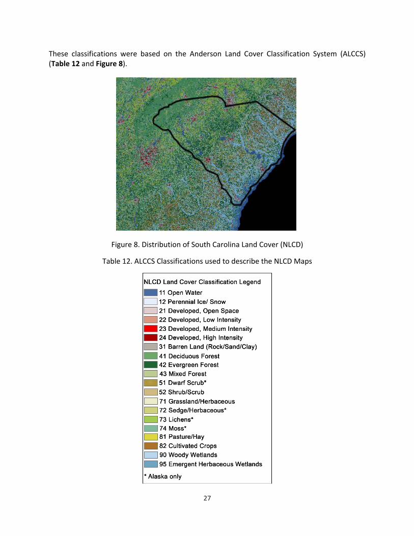
27

These classifications were based on the Anderson Land Cover Classification System (ALCCS) (Table 12 and Figure 8).

Figure 8. Distribution of South Carolina Land Cover (NLCD)

Table 12. ALCCS Classifications used to describe the NLCD Maps

28

Because the identification number given to each pixel had no quantifiable meaning, it needed to be converted into a scale that gave meaning to each of the land classifications. The ALCCS used to describe the pixels from the NLCD was matched to the South Carolina Requirements for Hydraulic Design guides for the runoff coefficient used in the rational method. The rational method is shown by the following equation:

Q = C * I * A * Cf (Eq. 1)

where: Q = discharge (cfs)

C = runoff coefficient

I = rainfall intensity (in/hr)

A = drainage area (acres)

Cf = recurrence interval coefficient

This equation is used to determine the required discharge capacity of various drainage infrastructures across South Carolina. The recurrence interval coefficient is arbitrary as it is the same for each culvert, and the mapped precipitation from the NOAA database can be an estimate to the relative rainfall intensity; however, the drainage area was difficult to estimate. With no indication of the size of the basin or body of water which feeds a specific culvert, the full equation cannot be predicted. The runoff coefficients used to estimate required discharge from the SCDOT Requirements for Hydraulic Design are shown in Table 13 and the corresponding runoff coefficient assigned to the ALCCS designations shown in Table 14.

Table 13. South Carolina Runoff Coefficients Used in Hydraulic Design

Description (SCDOT) Runoff Coefficient Description (SCDOT) Runoff CoefficientPavements & Roofs 0.90 Side Slopes, Earth 0.60

Earth shoulders 0.50 Side Slopes, Turf 0.30Drives & Walks 0.75 Median Areas, Turf 0.25

Gravel Pavements 0.50 Cultivated Land, Clay & Loam 0.50City Business Areas 0.80 Cultivated Land, Sand & Gravel 0.25

Unpaved Road, Sandy Soils 0.34 Industrial Areas, Light 0.50Unpaved Road, Silty Soils 0.35 Industrial Areas, Heavy 0.60Unpaved Road, Clay Soils 0.40 Parks & Cemeteries 0.10Aparment Dwelling Areas 0.50 Playgrounds 0.20

Suburban, Normal Residential 0.45 Woodland & Forest 0.10Dense Residential Sections 0.60 Meadows & Pasture Land 0.25

Lawns, Sandy Soils 0.10 Unimproved Areas 0.10Lawns, Heavy Soils 0.17 Rail Yards 0.25

Grass Shoulders 0.25 Expressways & Freeways 0.00

29

Table 14. ALCCS Pixel Data and Corresponding Runoff Coefficient from SCDOT

Once the parameters were mapped and converted into a quantifiable and meaningful value, the pixel data could be consolidated into larger areas that could be applied to a culvert. With each pixel only covering an average of 9,000 square feet (0.000325 square miles) per pixel, mapping the runoff coefficient of a single pixel to each culvert would likely result in some significant error and wouldn’t capture the effect of the surrounding area as each culvert’s runoff coefficient would be the average of the drainage area supplying the associated stream or river. Consequently, a square area of 25 pixels by 25 pixels was averaged to give a more representative sample of the average runoff coefficient. The new area covered by each data point corresponds to approximately 566,500 square feet, approximately 0.20 square miles, or 128 acres. These data points were then used to assign a culvert an average runoff coefficient for the surrounding 0.20 square miles using the nearest pixel associated with the culvert’s latitude and longitude.

Input Variable Combinations

In producing the most effective model, it is important to determine which combinations of input variables are most effective at predicting various output variables. Certain outputs may be better predicted using a more diverse or complex combination of input variables. In order to organize the testing of these models and to limit the number of trials for each model, a table of the available input variable was created (Table 15). These inputs were then combined to form trial models that would be evaluated to determine which models produced the best

Pixel ID Description (NLCD) Runoff Coefficient SCDOT Description11 Open Water 0.00 --12 Perennial Ice/Snow 0.00 --21 Developed, Open 0.45 Suburban, Normal Residential22 Developed, Low 0.50 Aparment Dwelling Areas

23 Developed, Medium 0.55Aparment Dwelling Areas/ Dense Residential Sections

24 Developed, High 0.60 Dense Residential Sections

31Barren Land

(Rock/Sand/Clay)0.40 Unpaved Road, Clay Soils

41 Deciduous Forest 0.10 Woodland & Forest42 Evergreen Forest 0.10 Woodland & Forest43 Mixed Forest 0.10 Woodland & Forest51 Dwarf Scrub 0.10 Woodland & Forest52 Shrub/Scrub 0.10 Woodland & Forest71 Grassland/Herbaceous 0.25 Meadows & Pasture Land72 Sedge/Herbaceous 0.25 Meadows & Pasture Land73 Lichens 0.25 Meadows & Pasture Land74 Moss 0.25 Meadows & Pasture Land81 Pasture/Hay 0.30 Side Slopes, Turf82 Cultivated Crops 0.40 Unpaved Road, Clay Soils90 Woody Wetlands 0.00 --

95Emergent Herbaceous

Wetlands0.00

--0 No Description 0.00 --

30

results as far as predicting the ten associated output variables (Table 16). The first ten combinations of inputs contain only variables that are linearly added to give the final prediction. The last three combinations of variables have a special variable that is a multiplicative combination of two or more variables. A neural network’s hidden neuron layer can be used to determine some of the more complex relationships between input variables; however, a logistic regression model requires the manipulation of such inputs by the user. After the 13 original combinations had been evaluated, the most accurate predictive model was used for each culvert type and output.

Table 15. Possible Input Variables and Assumed Importance

Variable Name ID # Assigned ImportanceAge 1 1pH 2 1

Runoff Coefficient 3 1Temperature 4 1Precipitation 5 1Num Barrels 6 2Culvert Shape 7 2

Width 8 2Height 9 2Length 10 2

Inlet End Type 11 3Inlet End Treatment 12 3

Inlet Apron Type 13 3Outlet End Type 14 3

Outlet End Treatment 15 3Outlet Apron Type 16 3

INPUT VARIABLES

31

Table 16. Combinations of Input Variables Tested

3.4 Deterioration Modeling Effort

3.4.1 Logistic Regression Analysis

In order to create the logistic regression models for each of the 13 combinations, the MATLAB built‐in function mnrfit was used. The function creates the coefficients of a multinomial logistic regression for a set of given inputs and corresponding outputs using the maximum log‐likelihood function. The coefficients that were returned from the fitting function were used in the built‐in MATLAB function, mnrval which created a probabilistic estimate based on the inputs of an associated culvert and the coefficients of the model that had been created. The result of this function is a probability distribution for each culvert giving an indication of the likelihood that a culvert is rated 1‐5. Assuming a linear relationship between the culvert ratings means that a non‐integer estimate was produced using the probability distribution and the value of the associated output, 1‐5. This predicted value can be compared to the measured output value and the statistical indicators of the effectiveness of the model can be calculated. In the case of each of the 13 combinations, the area under the ROC curve that was produced for each model was the primary indicator of the accuracy of the model. The selection of this criteria was based largely on the versatility of the ROC curve in determining a model’s ability to separate the data in distinct categories.

The 13 combinations of input variables were used to create 13 models, each addressing 6 culvert types and 10 output variables for a total of 780 models. For each of the models four ROC curves were created to address the model’s ability to separate an output rating of 1 from 2‐5, 1‐2 from 3‐5, 1‐3 from 4‐5, and 1‐4 from 5. The area underneath these curves can range from 0.5 to 1.0, with a higher score indicating a more accurate model. An ROC curve can produce an area under the curve of 0.0 usually indicating that the model cannot predict that

Combination ID Input Variables Combined Inputs1 1,2,3,4,5 --2 1,2,3,4 --3 1,2,3,5 --4 1,2,4,5 --5 1,3,4,5 --6 1-5,8,9,10 --7 1-5,6 --8 1-5,7 --9 1-5,11-16 --10 1,2,4 3 x 511 1,2,4 3 x 5 / 812 1,2,4 (3 x 5)/(8 x 9)13 1-5,6-10 --

COMBINATIONS

32

specific value, because there is not a culvert with that specific rating. For some of the culverts with fewer responses, this became an issue in determining the effectiveness of a model. Because this problem is independent of the combination of input variables used to create this model, the ROC curves could still be used as a measure of accuracy. In other cases where the number of observed culverts remained low, a large number of input variables can make it impossible to produce a model whose log‐likelihood function converges. Similarly, when too few or insignificant input variables were used, the log‐likelihood function would not converge. In these cases, an area under the ROC curve of 0.0 could be possible and understood to indicate a category where fewer responses were available.

The results of the 13 models addressing the 6 culvert types and 10 output variables is shown were Table 17. The values corresponding to the maximum area under the 4 ROC curves for each model is highlighted indicating the best combination of input variables.

33

Table 17. Area under Curve Results (Logistic Regression)

1 10 11 12 13 2 3 4 5 6 7 8 9 Max AreaCracked 2.592 2.439 2.421 2.363 2.672 2.428 2.313 2.560 2.550 2.656 2.601 2.633 2.723 9

Separated 2.457 2.382 2.356 2.583 2.924 2.377 2.244 2.457 2.464 2.827 2.466 2.728 2.732 13Corrosion 2.702 2.541 2.526 2.444 2.781 2.546 2.500 2.672 2.687 2.791 2.701 2.737 2.845 9Alignment 2.762 2.604 2.585 2.544 2.822 2.593 2.409 2.753 2.752 2.781 2.773 2.845 2.938 9

Scour 2.941 2.671 2.655 2.686 2.904 2.652 2.638 2.945 2.940 2.924 2.946 2.945 2.993 9Sedimentation 2.807 2.754 2.732 2.758 2.945 2.751 2.416 2.791 2.810 2.921 2.834 0.000 2.956 9

Vegetation 2.391 2.229 2.314 2.271 2.458 2.244 2.296 2.373 2.358 2.494 2.400 2.400 2.572 9Erosion 2.838 2.735 2.720 2.856 3.101 2.724 2.287 2.838 2.827 3.038 2.856 2.907 3.081 13

Blockage 2.367 2.268 2.271 2.229 2.455 2.260 2.240 2.352 2.324 2.459 2.366 2.371 2.611 9Piping 2.478 2.378 2.408 2.375 2.729 2.378 2.312 2.431 2.474 2.682 2.539 2.530 2.826 9

Cracked 2.615 2.431 2.412 2.523 2.977 2.472 2.399 2.600 2.582 2.940 2.683 2.674 0.000 13Separated 2.873 2.716 2.755 2.850 2.955 2.784 2.646 2.745 2.732 3.202 2.935 2.840 0.000 6Corrosion 2.798 2.560 2.488 2.808 3.147 2.577 2.765 2.751 2.606 3.157 2.806 2.866 0.000 6Alignment 3.295 2.899 2.859 3.080 3.226 2.931 3.054 3.265 3.258 3.171 3.299 3.328 0.000 8



Blockage 2.818 2.455 2.460 2.443 2.667 2.456 2.506 2.777 2.594 2.745 2.803 2.661 0.000 1Piping 2.776 2.247 2.371 2.627 2.950 2.241 2.581 2.775 2.788 2.898 2.801 2.839 0.000 13



Vegetation 3.072 2.856 3.296 1.000 1.667 2.837 2.986 2.861 2.942 1.750 2.534 0.000 0.000 11Erosion 0.000 0.000 0.000 0.000 0.000 0.000 0.000 0.000 0.000 0.000 0.000 0.000 0.000 --

Blockage 1.000 0.938 0.875 1.000 1.000 0.938 1.000 1.000 1.000 1.000 1.000 0.000 0.000 1Piping 1.000 1.000 1.000 0.000 0.000 1.000 1.000 1.000 1.000 0.000 1.000 0.000 0.000 1


Scour 1.889 1.833 1.750 1.643 1.500 1.389 1.944 1.467 1.622 1.643 1.889 0.000 0.000 3Sedimentation 0.000 0.000 0.000 0.000 0.000 0.000 0.000 0.000 0.000 0.000 0.000 0.000 0.000 --

Vegetation 2.761 3.194 3.289 2.677 2.700 3.271 3.114 2.936 3.154 0.000 3.171 0.000 0.000 11Erosion 0.000 0.000 0.000 0.000 0.000 0.000 0.000 0.000 0.000 0.000 0.000 0.000 0.000 --

Blockage 1.889 1.889 1.781 1.679 1.000 1.833 1.889 1.528 1.722 0.000 1.889 0.000 0.000 1Piping 1.958 1.958 1.857 1.444 1.000 1.917 1.958 1.483 1.875 1.889 1.958 0.000 0.000 1




Blockage 2.298 2.384 2.371 2.218 2.575 2.385 2.286 2.214 2.334 2.514 2.417 2.321 0.000 13Piping 3.347 3.257 3.318 3.179 3.435 3.270 3.148 3.445 3.224 3.477 3.344 3.357 0.000 6




Blockage 2.756 2.740 2.741 2.692 2.740 2.772 2.735 2.636 2.505 2.988 2.743 0.000 0.000 6Piping 2.602 2.801 2.600 2.366 2.474 2.773 2.785 2.453 2.391 3.319 2.586 0.000 0.000 6

Total Models 10 2 2 0 13 1 1 2 1 11 5 1 8 57

Mixed

COMBINATION NUMBER

RCP

CMP

CAP

HDPE

Masonry

34

3.4.2 Artificial Neural Networks

Like the logistic regression, the 13 combinations of input variables were used to create a total of 780 total neural network models. The three general functions governing the behavior of the neural network model are the weighting function, the bias function, and the transfer function. The transfer function is effected by the number of neurons used to model the relationships between both the input variables and each other and the input variables and the output variables. Because these relationships can often be complex, the number of neurons used in the transfer was varied from 1 neuron to 10 neurons. The creation of the neural network is based on the MATLAB built‐in Neural Network toolbox. The toolbox allows the user to specify the performance function (mean‐squared error and mean‐absolute error); however, in an attempt to stay consistent with the measure of the success of the predictive models between logistic regression and neural network models, the ROC curves were created with each of the models. The associated total area under the four ROC curves was used as the measure of the performance of the models. In each case, the maximum area under the curve was used to determine how many neurons created the best model. Similarly, the best of the 13 combinations of input variables was used to determine the optimal input variable combination (Table 18).

35

Table 18. Area Under Curve Results (Artificial Neural Network)

1 10 11 12 13 2 3 4 5 6 7 8 9 Max AreaCracked 2.865 2.747 2.696 2.647 2.806 2.750 2.608 2.834 2.881 2.836 2.897 2.883 2.772 7




Blockage 2.685 2.580 2.571 2.447 2.650 2.560 2.495 2.615 2.573 2.590 2.610 2.597 2.724 9Piping 2.859 2.821 2.710 2.685 2.831 2.842 2.711 3.004 2.766 2.759 3.056 2.912 2.995 7




Blockage 2.980 2.762 2.749 2.620 3.071 2.724 2.678 3.014 2.723 2.988 3.000 2.837 3.084 9Piping 3.179 3.012 3.141 3.208 3.161 3.108 3.037 2.953 3.061 3.140 3.030 3.142 3.083 12



Vegetation 2.802 2.988 2.892 2.000 2.417 2.912 2.679 3.123 3.089 2.500 2.995 2.980 3.183 9Erosion -- -- -- -- -- -- -- -- -- -- -- -- -- --

Blockage 1.000 1.000 1.000 1.000 1.000 1.000 1.000 1.000 1.000 1.000 1.000 1.000 1.000 1Piping 1.000 1.000 1.000 0.000 0.000 1.000 1.000 1.000 1.000 0.000 1.000 1.000 1.000 1



Vegetation 2.699 3.067 2.919 2.894 3.000 2.917 2.765 3.169 2.969 2.967 2.889 2.699 3.030 4Erosion -- -- -- -- -- -- -- -- -- -- -- -- -- --

Blockage 1.722 1.944 1.628 1.750 1.889 1.917 1.861 1.417 1.833 2.000 1.611 1.722 1.889 6Piping 1.958 2.000 1.651 1.417 1.944 2.000 1.958 1.733 1.817 2.000 1.958 1.958 1.833 10




Blockage 3.093 2.986 3.013 2.920 3.025 2.987 2.867 2.935 3.038 3.030 2.987 2.965 2.949 1Piping 3.547 3.540 3.534 3.614 3.376 3.499 3.384 3.695 3.552 3.548 3.588 3.477 3.714 9




Blockage 2.989 2.886 2.906 2.891 3.018 2.978 2.739 2.997 3.013 3.090 2.964 3.065 2.948 6Piping 3.046 2.929 3.023 2.622 3.545 2.858 3.158 2.866 2.668 3.530 2.783 3.423 3.174 13

Total Models 14 2 2 1 6 0 0 5 0 5 6 3 14 58

Mixed

COMBINATION NUMBER

RCP

CMP

CAP

HDPE

Masonry

36

Additional Model Modifications

Using the best model input combinations for both the logistic regression and the artificial neural network two final models addressing the six different culvert types and ten different output variables. These two models can, at this stage, give a prediction of the desired output on a continuous sale from 1.0‐5.0. In order to further develop the model as an efficient tool to determining the culverts in need of physical assessment, it is important to determine the optimal threshold of allowable falsely identified good condition and poor condition culverts. For example, the cost of examining a large percentage of culverts that may be in good condition needs to be limited; however, the fewer culverts that are marked as poorly rated culverts, the more culverts in need of inspection may be missed. When using ROC curves as an indication of a model’s accuracy, it is important to note that the ROC curve denotes the ability for the model to separate the data into groups while showing the tradeoff between true positive results and false positive results. Using an ROC curve allows the user to select a threshold value after the model is created that indicates the approximate amount of false positive results to be expected by the model.

Selecting the appropriate threshold can be done through two primary methods. The first of which weights the cost of a false positive and false negatives in a cost matrix. The cost matrix that is used to determine the optimal threshold point on the ROC curve is shown by Table 19.

Table 19. Cost Emphasis Matrix

In this matrix, the positive classification represents culverts that are less than or equal to a given output (1‐4). Conversely, the negative category represents culverts that are greater than a given output rating. For example, at an output rating of 3, positive culverts are denoted as culverts less than or equal to 3, while negative culverts are shown as those culverts greater than 3. The ratio of these scores gave an indication of the consequence of falsely identifying culverts with better ratings as having a poor rating, as well as denoting culverts that are in need of inspection and repair as in good condition. In the case of the South Carolina Department of Transportation, the consequence of failing it identify a culvert in need of repair (N|P) would be much greater than the consequence of identifying a culvert that is in good condition as one in need of repair (P|N). Typically, there is no cost associated with correctly identifying good condition or poor condition culverts; however, the model can account for situations that would require these values to be non‐zero.

The second method used to determine the threshold point is by attempting to maximize the percentage of culverts that were placed in the correct category. By using only the cost matrix, the output of the model may categorize all culverts for inspection rendering the model useless. In the case of the logistic regression model and the artificial neural network model, attempting to use the cost matrix as a method for determining the optimal threshold point was ineffective

Actual\Model Positive NegativePositive P|P N|PNegative P|N N|N

37

as the model set the threshold point at 0 false positives and 0 true positives. Because each of the models behave differently, setting a single threshold in terms of a percent of culverts is unlikely to serve each of the culverts well. Imposing realistic limits on the amount of culverts prescribed for inspection was important to the feasibility of the model. These final model modifications and thresholds are set for each of the six culvert types and ten output categories by using the results of the likelihood function. Using this result allows for the best separation of the data. The overestimation of a culvert’s output rating can be corrected for by fitting the observed output versus the predicted output to a regression. This step was most easily done after the composite score was calculated as it meant the user only has to deal with a single value.

Preliminary Conclusions

Figure 9. Relationship between Observed Culverts and Average Number of Inputs

The distribution of most effective models clearly follows the general rule that more data points (culverts) requires a model with more input variables. In cases where the number of observed culverts were smaller, models that utilized fewer input variables were more successful. This trend, illustrated in Figure 9, can be shown with a logarithmic relationship for logistic regression models. This conclusion helped to minimize the time spent testing future combinations of input variables for logistic regressions. Future combinations with more input variables could only be tested on RCP culverts, while combinations with fewer inputs could be tested on HDPE and CAP culverts. CMP, masonry, and mixed/other culverts were tested for all additional models as their dependence on the amount of input variables varied more with the type of output that was being predicted. There were no such relationships present in the results of the artificial neural network models. In addition, there were no relationships found between the number of neurons used to determine the final output ratings and the number of inputs in the final model.

38

In a comparison of the performance measures, there was almost no matches in the best combinations between the mean squared error performance indicator and the area under the ROC curve indicator. Only two of the sixty models (3.33%) found the same combinations of input variables to have combination of inputs yield the best model for both mean squared error and area under the ROC curve. This conclusion was reasonable because the two performance measures are based on fundamentally different principles. The mean squared error attempts to find the model that creates the closest error for each individual culvert based on a continuous scale. Because the data represented by the SCDOT database has culverts with average ratings above four, the data is skewed toward the higher rated culverts. With this information, the mean squared error performance based models are more likely to predict higher ratings in an effort to reduce overall error. Models based on the area under the ROC curve are viewed as more effective when they can sort the culverts into discrete categories 1‐5. The purpose of these models is more in line with the performance characteristics of ROC curves. Ranking the culverts and identifying those culverts in most need of assessment was more important than correctly predicting the rating of culverts, especially those culverts in better condition.

3.5 Primary Outcomes: Model Discussions, Comparisons, and Conclusions

Generalized Effect of Input Variables

Despite the complexities in determining the assessment rating of culverts using logistic regressions and artificial neural networks, conclusions can be made from the coefficients of the model. In the case of the logistic regression, the influence of each input variable, whether positive or negative can be tracked through these coefficients. In total, 15 unique input variables in the various combinations for each of the logistic regression and artificial neural network models. For each of the inputs their impact on a specific output variable can be either positive, negative, or neutral. The complexity of the problem increases in that each input variable can have a defined impact over only portion of the spectrum of assessment values 1‐5. A specific input may significantly impact the decline of a culvert from a rating of 5 to 4, but it may have no effect on the deterioration from 2 to 1. In the case of the dummy variables, this becomes problematic as each coefficient only addresses the binary nature of a single quantifier. To avoid this, the beta value for each possible variable needed to be determined. Once all of this information was received for each of the six culvert types, it could be used to draw conclusions about each variables contribution to the output variables. For example, a coefficient value of 1.25 for the input variable pH would correspond to an increase in the culvert rating of exp(1.25) or 3.49 for each unit increase in pH with all else equal.

From this information, there were several trends that could be observed for each of the logistic regression models. Each of the trends fell into one of six categories. These trends are also illustrated in Figure 10.

Trend 1: Input variable has an undetermined effect on the output

Trend 2: As culvert deteriorates, impact of variable decreases*

39

Trend 3: As culvert deteriorates, impact of variable increases*

Trend 4: Input has little effect on variable**

Trend 5: Input effect magnified at rating category 2 and/or 3 but generally positive or negative*

Trend 6: Impact of variable remains constant as culvert deteriorates *These trends can have a positive or negative effect on variables **Because input range changes based on the type of input, a lower value may be misleading (a unit increase may be more significant in pH as compared to a unit increase in precipitation)

Figure 10. Trend Types for Input Coefficients of Logistic Regression Models

The trend of each input variable was assigned for all inputs of each model. There were a total of 10 trend classifications for each input variable as trends 2, 3, 5 and 6 could be considered positive or negative based on the value of the coefficient. With each variable categorized, the general effect of the input variables could be shown to be positive, negative, or having small effects on the output. An attempt was then made to understand these effects and determine if they are in line with assumptions and practices common to design and maintenance of culverts.

Primary Variables

The four primary variables that were mapped to each culvert and used in most models were pH, runoff coefficient, temperature, and precipitation. Figure 11 captures the general effect of these variables on the outputs of the model. In these figures, which aim to capture the generalized effect of an input variable on all output variables, the positive and negative effects must be interpreted in terms of the equation that governs the prediction of the output variable.

lnP Output≤k

P Output>k=β0+β1X1+β2X2+…+βnXn for k=1,2,3,4 (Eq. 2)

40

Figure 11. Distribution of Effect of Primary Input Variables

In this equation a positive value of β increases the relative probability of the output variable being less than the classification in question (1, 2, 3 or 4). Through this example, a variable indicated as having a negative value increases the probability that a given output variable is greater than the threshold. In examining the generalizations of the impacts of the primary variables, most of these variables are shown to have a negative value. Consequently, a decrease in the value for these variables would correspond to an increase in the probability that the culvert is in better condition than the indication point.

It is important to determine if the negative values for pH, runoff coefficient, temperature, and precipitation follow the general logic of the effects of these variables. Proving that an increase in the pH would help a culverts rating, especially its corrosion rating, follows the logic that more acidic water is worse for a culvert’s health. Similarly, a negative value associated with the temperature coefficient, particularly in structural related models indicates that the places in South Carolina that are colder and more susceptible to freeze and thaw cycles, would have a negative effect on the culvert’s output ratings. These trends can also be observed in a graph of the predicted outputs as a function of the primary input variables.

41

The negative values associated with the input variables of runoff coefficient and precipitation are not as easily explained with intuition. In the case of both runoff coefficient and precipitation, an increase in these inputs would mean an increase in demand on the culvert. While this effect can be explained for some output variables like blockage and vegetation where an increase in the amount of water would decrease the likelihood for excess vegetation, sedimentation, and culvert blockage, other output variables would not logically benefit from an increased amount of water. Alignment, cracking, and erosion would logically see a reduction in output rating with an increase in the precipitation and runoff coefficient when examined in a global sense. It was important to note that the life cycle of a culvert is dependent on the localized conditions that effect the demand, and the input variables used to predict the output capture a more global effect of each culvert.

These general effects were confirmed with graphs isolating a culvert’s predicted output score were plotting against each primary variable. To give reference, the actual distribution of ratings is shown in red, while the predicted rating was shown in red in Figure 12.

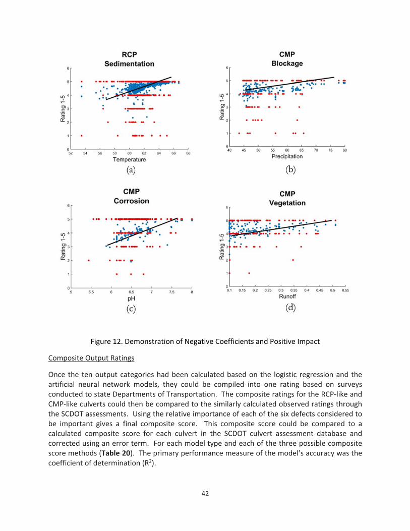
42

Figure 12. Demonstration of Negative Coefficients and Positive Impact

Composite Output Ratings

Once the ten output categories had been calculated based on the logistic regression and the artificial neural network models, they could be compiled into one rating based on surveys conducted to state Departments of Transportation. The composite ratings for the RCP‐like and CMP‐like culverts could then be compared to the similarly calculated observed ratings through the SCDOT assessments. Using the relative importance of each of the six defects considered to be important gives a final composite score. This composite score could be compared to a calculated composite score for each culvert in the SCDOT culvert assessment database and corrected using an error term. For each model type and each of the three possible composite score methods (Table 20). The primary performance measure of the model’s accuracy was the coefficient of determination (R2).

43

Table 20. Coefficient of Determination (R2)

The first observation from the composite score analysis was that each culvert type had a significant advantage using one model type versus another. For RCP, CMP, masonry, and mixed/other culverts, the artificial neural network model proved to produce better results. For the CAP and HDPE models, the logistic regression model proved to explain more of the variation. A possible reason for this occurrence is the lack of data that can be found in the CAP and HDPE categories. When the amount of information was less, the simplest model did the best job of explaining the causes and effects of the input variables. The linear addition of the input variables proved to be the best way to describe the condition of the culvert when only a few culverts were available. This phenomenon may also have been the case because all of the data was used to create the logistic regression models. Without any validation of the model with unused data, a significant bias can be introduced when there are only a few data points.

The second observation was that there was no clear method of developing a composite score that proved to be better than the others. For all culvert types except HDPE, the top two methods for determining composite score were within 10% of each other. This could be partially due to the fact that the two DOT estimates for the relative severity of defects showed only slight differences for RCP and CMP culverts. Furthermore, the differences between the DOT estimates and a simple average of the six output variables assumed to be significant were relatively small as well. Moving forward, all three models will be available for the user to select. The user could also input their own set of weighting criteria; however, there would not be an associated regression analysis that corrects this estimate.

A final observation of the composite score analysis was the relatively low magnitude of the coefficient of determination in comparison to previous research. For the category with the most information, RCP, the coefficient of determination was the worst (0.252). This means that only 25.2% of the variability in the data for RCP culverts is captured by the current model. A possible reason for this poor model could be too much data used to create the model. Because the distribution of the data from the SCDOT Culvert Assessment Database was significantly skewed to the culverts with ratings of 4 and 5, and the model attempts to reduce the amount of total error produced by the regression, the model is biased towards the higher rated culverts. In models where the distribution of culverts had closer to equal amounts of culverts in each category, the coefficient of determination was higher.

44

Using the tools available in a regression analysis allows for the error term to be included in the model. When the user inputs a culvert’s information, the logistic regression or artificial neural network model will produce an estimate based on the functions that define that particular model. The prediction will then be used in the linear regression analysis to produce a final prediction of the culvert’s composite score. In addition to this prediction, the variability in the data will allow for a range of predictions to be made. This range deals with the variability at a specific point in the regression analysis. As shown in Figure 13 representing CMP culverts and a composite scored determined by the DOT Estimate 1 method, the boundary for the culverts can be seen. The upper and lower boundary look to capture one standard deviation from the mean value predicted by the regression. This additional parameter can serve to allow the user to have an estimate as to the lower and upper bound of the composite score.

Variability in the Models

The distribution of the standard deviation for each model can serve to help understand how well the model captures the data with the single prediction. The larger the standard deviation, the less the single prediction accounts for more of the data. For most of the models and composite score weights the average standard deviation across the spectrum of possible answers (1‐5) was between 0.3 and 0.6. In a case where the standard deviation is 0.5, approximately half of the variation is captured in a range of 1.0. A complete breakdown of the standard deviation associated with each of the composite scores and culvert types is shown in Table 21. The average standard deviation was determined by finding the standard deviation of equally spaced points from a predicted output of 3 to a predicted output of 5. Because there was much more variability in the model below an estimation of 3 and very few entries, an average of equally spaced points between 1 and 5 would not give an accurate indication of the average standard deviation. The increased variability can be seen where the lines indicating the standard deviation grow farther apart as the predicted value decreases. This is to be expected as there are fewer data points lower on the scale and the models ability to predict them has decreased.

45

Figure 13. CMP Composite Score DOT Estimate 1 with Error Term

Table 21. Standard Deviation for Each Model Type and Composite Weight

ANN LogRegDOT Est 1 - RCP 0.479 0.500DOT Est 2 - CMP 0.503 0.515

All Equal 0.497 0.514DOT Est 1 - RCP 0.524 0.630DOT Est 2 - CMP 0.549 0.639





All Equal 0.422 0.540

Masonry

Mixed

RCP

CMP

CAP

HDPE

46

3.6 Model Conclusions

Weaknesses of Models

When considering the finalized models, it was important to understand the limitations and weaknesses of its prediction capabilities. The first major weakness of the model was the spatial bias that was created when the mapped input variables were assigned to the culverts. Because these mapped inputs varied spatially using linear interpolation, two culverts that were located very close together would receive nearly identical values for temperature, precipitation, pH, and estimated runoff coefficient. With all other physical properties like culvert type, culvert shape, and dimensions equal, these culverts would likely receive a nearly equal estimate for the output variables. With no additional way to differentiate these culverts such as age, any variation in the ratings of these culverts would not be captured by the model.

In addition to the localized spatial bias, the model may be affected by spatial bias in the global sense. Where models were created with fewer culverts (HDPE and CAP) the model could separate these culverts and assign ratings based entirely on spatial variation illustrated in Figure 14. In this case, the model would predict the culvert rating based on this spatial bias. Any validation performed on this model shows that the predition capabilities for the model are very poor. This was underscored by the neural network’s poor performance on culvert types with fewer data points as the neural network process includes validation.

Figure 14. Spatial Bias Potential in Models with Fewer Input Culverts

In addition to the spatial bias, there is a bias in the model towards the highly rated culverts. Because the distribution of culvert output ratings was significantly skewed towards the higher rated culverts (Table 22). When using models that incorporate all data or a percent of the entire data, the model sought to maximize the performance indicators. With more of the data receiving higher rating, the model prioritizes accurately estimating these data points at the expense of over‐predicting the lower rated culverts. Some of this bias is removed by emphasizing the ROC curves and the models ability to separate these culverts from the higher

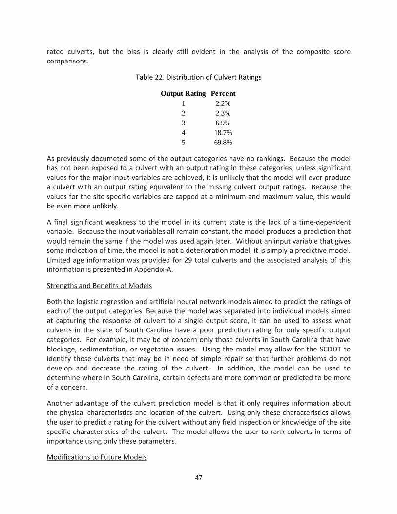
47

rated culverts, but the bias is clearly still evident in the analysis of the composite score comparisons.

Table 22. Distribution of Culvert Ratings

As previously documeted some of the output categories have no rankings. Because the model has not been exposed to a culvert with an output rating in these categories, unless significant values for the major input variables are achieved, it is unlikely that the model will ever produce a culvert with an output rating equivalent to the missing culvert output ratings. Because the values for the site specific variables are capped at a minimum and maximum value, this would be even more unlikely.

A final significant weakness to the model in its current state is the lack of a time‐dependent variable. Because the input variables all remain constant, the model produces a prediction that would remain the same if the model was used again later. Without an input variable that gives some indication of time, the model is not a deterioration model, it is simply a predictive model. Limited age information was provided for 29 total culverts and the associated analysis of this information is presented in Appendix‐A.

Strengths and Benefits of Models

Both the logistic regression and artificial neural network models aimed to predict the ratings of each of the output categories. Because the model was separated into individual models aimed at capturing the response of culvert to a single output score, it can be used to assess what culverts in the state of South Carolina have a poor prediction rating for only specific output categories. For example, it may be of concern only those culverts in South Carolina that have blockage, sedimentation, or vegetation issues. Using the model may allow for the SCDOT to identify those culverts that may be in need of simple repair so that further problems do not develop and decrease the rating of the culvert. In addition, the model can be used to determine where in South Carolina, certain defects are more common or predicted to be more of a concern.

Another advantage of the culvert prediction model is that it only requires information about the physical characteristics and location of the culvert. Using only these characteristics allows the user to predict a rating for the culvert without any field inspection or knowledge of the site specific characteristics of the culvert. The model allows the user to rank culverts in terms of importance using only these parameters.

Modifications to Future Models

Output Rating Percent1 2.2%2 2.3%3 6.9%4 18.7%5 69.8%

48

For the model to continue to improve in its capabilities to predict the output of culverts, modifications are necessary. A continued analysis to the impact of the age of a culvert would allow for these models to be applied to all culvert types and likely produce more accurate models. Implementing the model would only be possible if the age of future culverts whose condition was desired also had a known installation date. With these models would come an expected increase in accuracy as well as a prolonged useful life of the model. If the model could take into account a time‐dependent variable, the model is no longer static and could produce more meaningful results in the future without an update in the parameters of each individual model.

Another important modification to the current model that could bring about an increase in the performance of the model would be using different portions of the data to train the original model. This would apply mostly to the models with a large amount of data. In these cases it may be advantageous to use equal amounts of data from each output category. Because nearly 90% of the data has an output score of either 4 or 5, the bias towards this data is significant. By forcing the model to treat each output equally, it may be more likely to capture the true trends in the data and deterioration of culverts.

In the final model, both the artificial neural network model and the logistic regression model will be available for the user to select and use. However, based solely on the coefficient of determination performance measure, one model is clearly better than the other for each of the culvert type (Table 23).

Table 23. Breakdown of Better Model

Review of Model Creations & Use

Figure 15 reviews the entire process of the predictive model’s creation and use.

Better ModelRCP ANNCMP ANNCAP LogReg

HDPE LogRegMasonry ANN

Mixed ANN

49

Figure 15. Model Overview and Usage

3.6 Chapter Summary

Logistic regression and artificial neural network models are developed to predict the ratings for each of the assessment output categories as per SCDOT’s culvert inspection manual. These categories include: cracking, separation, corrosion, alignment, scour, sedimentation, vegetation, erosion, blockage, and piping. The modeling effort entailed using the physical culvert information given in the inventory database of culverts and mapping the environmental characteristics including historical temperature, precipitation, pH, and estimated runoff coefficient. The predicted scores for each of the output categories were combined to give an overall composite score for each of the culverts. The models produced were shown to have a coefficient of determination of between 0.25 for poorly correlated models to a coefficient of determination 0.80 for better correlated models when comparing the predicted culvert score with the actual culvert score. Ultimately, the acquisition of information on the age of a large portion of the culverts would be desirable to further develop the model.

50

4. RISK‐BASED CULVERT RENEWAL PRIORITIZATION

4.1 SCDOT Culvert Inventory Analysis and Defect Categorization

The latest SCDOT’s culvert inventory database contained condition evaluation scores of various culverts that have been inspected over the past few years. The inspection procedure that is followed is detailed in the SCDOT’s Field Inventory and Inspection Guidelines manual published in 2011 (SCDOT, 2011). The assessment of culverts, as described in the Inspection Guidelines manual, is categorized into separate evaluations of inlet, outlet and barrel structures for each culvert. Eight criteria are specified for inspecting inlet and outlet structures each, while seven criteria are used for the inspection of the barrel. An assessment scale of 1 to 5 (5 representing best condition) has been specified with suggested descriptive assessment levels for each criteria. The inspection criteria are listed in Table 24 while the definitions of these criteria and suggested guidance for ratings are described in greater detail in SCDOT (2011).

Table 24. Criteria used by SCDOT for the assessment of culverts

Inlet/outlet Barrel

Alignment Corrosion

Erosion Cracked

Cracked Alignment

Separated Sediment

Scour Joint Separation

Vegetation Piping

Blocked Blocked

Corrosion

4.2 Survey of Other States

As part of this research project, a brief survey of culvert failure risk assessment is sent out to all the state DOTs. The survey is included in Appendix‐B of this report. The survey focused on the failure risk assessment of the barrel structure within a culvert. The survey identified specific structural defects, shown in Table 25, for each of reinforced concrete pipe (RCP) and corrugated metal pipe (CMP) that may eventually lead to the failure of the barrel. The participant’s opinion on the relative criticality of each defect type is separately solicited for RCP and CMP culverts using a qualitative scale. The definitions of the structural defects along with their threshold severities are specified in the survey to make it as explicit as possible. The definitions of the defects included in the survey are presented in Table 26 and their severities are defined in Table 27.

51

Table 25. Defects in RCP and CMP culverts that may lead to the barrel failure

Reinforced Concrete Pipe (RCP) Corrugated Metal Pipe (CMP)

Cracked Corrosion

Joint misalignment Joint misalignment

Joint inflow/infiltration Joint inflow/infiltration

Invert deterioration Invert deterioration

Bedding voids Bedding voids

Shape deformation

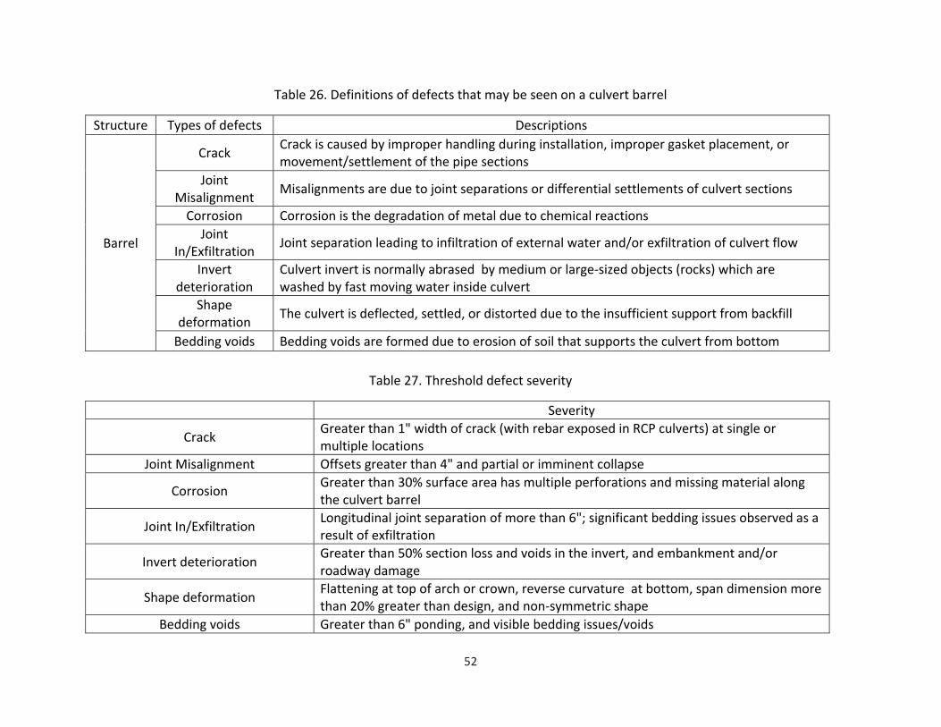
52

Table 26. Definitions of defects that may be seen on a culvert barrel

Structure Types of defects Descriptions

Barrel

Crack Crack is caused by improper handling during installation, improper gasket placement, or movement/settlement of the pipe sections

Joint Misalignment

Misalignments are due to joint separations or differential settlements of culvert sections

Corrosion Corrosion is the degradation of metal due to chemical reactions

Joint In/Exfiltration

Joint separation leading to infiltration of external water and/or exfiltration of culvert flow

Invert deterioration

Culvert invert is normally abrased by medium or large‐sized objects (rocks) which are washed by fast moving water inside culvert

Shape deformation

The culvert is deflected, settled, or distorted due to the insufficient support from backfill

Bedding voids Bedding voids are formed due to erosion of soil that supports the culvert from bottom

Table 27. Threshold defect severity

Severity

Crack Greater than 1" width of crack (with rebar exposed in RCP culverts) at single or multiple locations

Joint Misalignment Offsets greater than 4" and partial or imminent collapse

Corrosion Greater than 30% surface area has multiple perforations and missing material along the culvert barrel

Joint In/Exfiltration Longitudinal joint separation of more than 6"; significant bedding issues observed as a result of exfiltration

Invert deterioration Greater than 50% section loss and voids in the invert, and embankment and/or roadway damage

Shape deformation Flattening at top of arch or crown, reverse curvature at bottom, span dimension more than 20% greater than design, and non‐symmetric shape

Bedding voids Greater than 6" ponding, and visible bedding issues/voids

53

The survey participants were asked the following question for each pair of defects separately for RCP and CMP culverts: “How concerning is defect #1 compared to defect #2 with respect to barrel health while determining the need for its rehabilitation/replacement?” It has been specified that the defect severities be considered equivalent to the threshold levels presented in Table 27. The qualitative scale used in the survey for inputs comprises: “significantly less concerning,” “less concerning,” “somewhat less concerning,” “equally concerning,” “somewhat more concerning,” “more concerning,” and “significantly more concerning.”

The survey responses were initially analyzed for completeness and it was determined that only eight responses were complete enough to be included in further analysis. The eight complete responses were obtained from Arkansas Highway and Transportation Department, Indiana DOT, Ohio DOT, Iowa DOT, Maine DOT, Virginia DOT, Utah DOT, and South Dakota DOT. A few other responses were either incomplete or mere comments on the survey and the overall study methodology. The low response rate can be partly attributed to the fact that the survey was not a usual straight‐forward, objective Q&A type. Nevertheless, it should be noted that some of the responded DOTs have sponsored or participated in culvert infrastructure related studies in the past and their inputs are consequently deemed highly valuable.

The quantitative conversion scale, presented in Table 28, is used to translate the qualitative survey inputs to numeric values for quantitative analysis. Average of quantitative inputs over all responses for each pair of defects is calculated. The principles of Analytical Hierarchy Process (AHP) (Saaty, 1976) are employed for calculating the priority vector that determines the weightings of each defect type as a summary of the survey responses. Table 29 presents the results of the culvert failure risk assessment survey which indicates the relative weighting of defects that influence the overall failure risk of a culvert barrel. It should be noted that the defects “Joint misalignment” and “shape deformation” from the survey are combined to be one defect in order to be consistent with the defects used in the SCDOT’s culvert inventory database.

Table 28. Quantitative conversion scale used for the culvert failure risk assessment survey

Relative Importance Scale

Significantly less concerning 0.25 (or 1/4)

Less concerning 0.33 (or 1/3)

Somewhat less concerning 0.5 (or 1/2)

Equally concerning 1

Somewhat more concerning 2

More concerning 3

Significantly more concerning 4

54

Table 29. Criticality of various barrel defects

Reinforced Concrete Pipe (RCP) Corrugated Metal Pipe (CMP)

Defect Type Weightage (%) Defect Type Weightage (%)

Cracked 22.8 Corrosion 21.2

Joint misalignment 20.5 Joint misalignment & Shape deformation

33.6

Joint inflow/infiltration 23.4 Joint inflow/infiltration 18

Invert deterioration 20 Invert deterioration 17.7

Bedding voids 13.3 Bedding voids 9.5

4.3 Risk‐based Culvert Renewal Prioritization Model

The weightings for various defect categories, as shown in Table 29, are combined with the appropriate rating scores in the culvert inventory database to determine the overall criticality score of a given culvert using Eq. 3. The overall criticality will range between 0 and 1. It should be noted here that only the barrel defects are considered in the failure risk analysis and that the inlet and outlet defects are not.

∑ ∗ (Eq. 3)

C is the overall criticality score of a given culvert; WBj is the percentage weighting assigned to a barrel defect j (presented in Table 29); RBj is the rating score given to a given culvert for the defect j (between 1 and 5) as prescribed by the SCDOT culvert inspection manual.

The criticality score is combined with estimated failure consequences to determine the overall failure risk of a given culvert. Critical culverts lying under smaller roads may not have greater consequences when failed, but those lying under heavy‐traffic corridors will result in severe consequences posing significant risk. Failure consequences therefore will be proportional to the type of road under which the culvert is buried. Culverts with risk values greater than a threshold will be isolated for further inspection, or prioritized for repair.

4.4 Model Demonstration and Outcomes

The failure risk‐based prioritization model is demonstrated using the culvert assessment data available in the SCDOT’s culvert inventory database. All structural barrel defects in the assessment database are mapped with the defects included in the survey, as shown in Tables 30 and 31. A few defects included in the inventory, such as blocking and sediments, are excluded from this risk analysis, for they are not structural defects that directly influence the failure of the barrel.

55

Table 30. Defect mapping for RCP culverts

SCDOT inventory Survey

Cracked Crack

Alignment Joint Misalignment

Joint Separation Joint In/Exfiltration

Piping Bedding Voids

Erosion Invert deterioration

Table 31. Defect mapping for CMP culverts

SCDOT inventory Survey

Corrosion Corrosion

Alignment Joint Misalignment

+ Shape Deformation

Joint Separation Joint In/Exfiltration

Piping Bedding Voids

Erosion Invert deterioration

The SCDOT’s culvert inventory database contains assessment scores of about 5,000 RCP culverts and about 225 CMP culverts which are identified by a unique “Culvert ID.” The RCP culverts in the SCDOT’s culvert inventory database add up to a total length of 90.75 miles while the CMP culverts added up to about 4.37 miles. It should be noted that the inventory database contains assessments conducted only in the first phase of the campaign and therefore it does not cover all the culverts SCDOT is responsible for. These numbers by no means are proportional to the type of culverts SCDOT is responsible for. The assessment scores of the culverts for various defects are combined with the respective defect weightings in Tables 30 and 31 using Eq. 3 to obtain an overall criticality score (C) for each culvert.

The culvert inventory database also identified for each culvert the type of route under which it is buried under. The routes are classified into interstates (denoted by “I”), primaries (denoted by “US” or “SC”), and secondary (denoted by “S”). As noted previously in this chapter, the failure consequences of a culvert are roughly estimated using the type of route they serve. The consequence scores (FC) presented in Table 32 are used (upon discussion with the steering committee) to estimate culvert failure consequences. Figures 16 and 17 illustrate the distribution of RCP and CMP culverts by length, respectively, based on the routes types they are buried under.

56

Table 32. Failure consequence scores

Route Type Failure Consequence Score

I 1

SC 0.75

US 0.75

S 0.25

Figure 16. Route type distribution for RCP culverts measured by length

57

Figure 17. Route type distribution for CMP culverts measured by length

The criticality scores (Cj) are multiplied with the normalized failure consequence scores (FCj) to estimate the failure risk (Rj) of each culvert (j) in the inventory database using Eq. 4. The failure risk values will be in the range of 0 and 1.

∗ 1 (Eq. 4)

It was determined that about 61.3% of RCP culverts measured by length (≈ 55.1 miles) are at no risk as per the assessment scores in the SCDOT’s culvert inventory database. Figure 18 presents the distribution of RCP culverts measured by length based on their failure risk values. It should be noted that only those culverts with failure risk values of greater than zero are included in Figure 18. Out of the RCP culverts that are estimated to be at some risk, only about 4%, measured by length (≈ 1.42 miles), are found to have failure risk estimates ranging between 0.3 and 1, as can be observed from Figure 18. All such RCP culverts with failure risk estimates greater than 0.3 (59 in number) are identified and listed in Appendix‐C of this report in the decreasing order of their failure risk. It should be noted that a few RCP culverts had recorded assessment scores of zero in the SCDOT’s culvert inventory database and such culverts are excluded from the analysis presented in this report, for these entries were perceived to be errors in data recording.

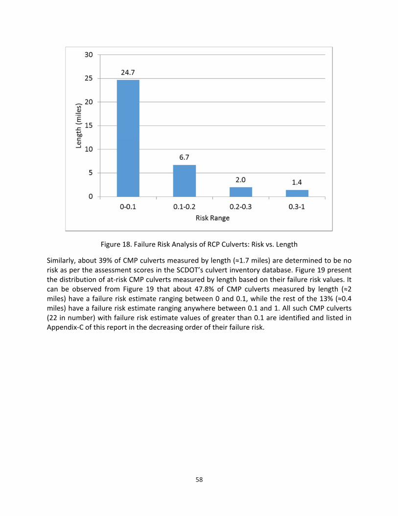
58

Figure 18. Failure Risk Analysis of RCP Culverts: Risk vs. Length

Similarly, about 39% of CMP culverts measured by length (≈1.7 miles) are determined to be no risk as per the assessment scores in the SCDOT’s culvert inventory database. Figure 19 present the distribution of at‐risk CMP culverts measured by length based on their failure risk values. It can be observed from Figure 19 that about 47.8% of CMP culverts measured by length (≈2 miles) have a failure risk estimate ranging between 0 and 0.1, while the rest of the 13% (≈0.4 miles) have a failure risk estimate ranging anywhere between 0.1 and 1. All such CMP culverts (22 in number) with failure risk estimate values of greater than 0.1 are identified and listed in Appendix‐C of this report in the decreasing order of their failure risk.

59

Figure 19. Failure Risk Analysis of CMP Culverts: Risk vs. Length

The failure‐risk based prioritization method identified the most critical RCP and CMP culverts from the list of assessed culverts that would require immediate attention for further inspection and/or renewal. The failure risk assessment is mainly dependent on the evaluation scores in the SCDOT’s culvert inventory database and the defect weightings derived from the responses of the survey conducted as part of this study. Furthermore, broad assumptions were made to estimate the failure consequences of various culverts depending on the type of route they are buried under. As SCDOT continues to monitor their culvert infrastructure and record assessment scores, this prioritization method can serve as a preliminary tool for systematically identifying the set of most critical culvert structures. The defect weightings and the failure consequence estimates can be easily modified to suit the needs of SCDOT as and when needed.

There are several limitations to the failure risk‐based prioritization approach developed and demonstrated in this project. Foremost is the limited number of survey responses that informed the defect‐weightings derived in this study. Due to the varied practices across several DOTs in evaluating culvert structures, it was difficult to capture various practical perspectives in a comprehensive manner through the survey conducted in this study. It was assumed that the defect severities as defined in the survey are representative of defects and their relative influence on the overall barrel condition. The lack of consideration of the inlet and outlet structures as part of the failure risk assessment is another limitation that may be addressed in the future. Another limitation is the uncertainty with respect to the consistency with which defect scoring is carried out, especially when multiple inspectors are engaged.

4.5 Chapter Summary

This chapter presented a failure risk‐based prioritization model for identifying the most critical culverts that may need immediate attention in terms of renewal planning. The prioritization

60

model is based on the principles of analytical hierarchy process (AHP) where in defect scores are combined with their respective relative weightings to estimate the failure risk of a culver barrel. The prioritization model would be mainly informed by the assessment scores from the SCDOT’s culvert inventory database and defect weightings derived from a survey conducted as part of this project. The prioritization model has been demonstrated using the latest culvert assessment inventory obtained from SCDOT to identify the most critical RCP and CMP culverts. The flexible prioritization model allows modification of defect weightings and failure consequence estimates by SCDOT staff as and when needed without much difficulty.

61

5. CULVERT RENEWAL GUIDANCE

Millions of culverts exist in the U.S., some of which are managed by State Departments of Transportation (DOTs) and others by local governments and U.S. Forestry Service. A majority of these culverts are made of reinforced concrete pipe (RCP), corrugated metal pipe (CMP), or high density polyethylene (HDPE) materials. As culvert pipes age, they deteriorate due to a combination of factors that include but not limited to: a) natural material degradation and subsequent loss of structural capacity, b) lack of proper maintenance, c) design defects or construction errors that weaken the system over time, and d) adverse environments (Yazdekhasti et al., 2014). Many existing culverts in the U.S. are in a deteriorated state having reached the end of their useful design life (Yang and Allouche, 2009). Due to the invisibility of buried culverts from the surface, they often get ignored until a problem such as road settlement or flooding arises. There have been several reported cases of culvert failures in the U.S. that caused the collapse of roads, posing a significant safety risk to motorists (Perrin Jr. and Jhaveri, 2004).

There are several technological, managerial and financial challenges to transportation agencies for adequately revamping or rehabilitating the culvert infrastructure. Technological challenges include the lack of appropriate technologies to fix all defects in an economical and reliable manner. Financial challenges include lack of adequate funding to invest in transportation infrastructure assets. Managerial challenges include lack of efficient, knowledge‐based decision‐making tools for the optimal management of culvert infrastructure. In an attempt to address some of the managerial challenges, this chapter describes an easy‐to‐use decision‐making tool called Culvert Renewal Selection Tool (CREST) for determining optimal renewal technique choices for a given application scenario.

Due to the increased traffic density on roadways and the resulting economic, societal, and environmental impacts of conventional open‐cut techniques, transportation agencies are increasingly looking to adopt trenchless techniques for addressing their culvert problems. Several trenchless repair, rehabilitation and replacement techniques (all three categories hereafter referred as “renewal” techniques) are considered as possible alternatives in this study. The objective of this chapter is to synthesize the performance of various popular culvert renewal techniques in order to develop and demonstrate a rational decision making tool for their optimal selection given an application scenario. The CREST model integrates the performance evaluation of various culvert renewal techniques with criteria preferences of the user by employing the principles of Analytical Hierarchy Process (AHP). The CREST model is demonstrated for various typical application scenarios that are grouped into renewal types (non‐structural, semi‐structural or full‐structural) based on the host culvert material, size, prevailing defect type and severity. The CREST model is subsequently validated using a novel practice‐based reflective validation approach in which real‐world culvert renewal preferences are compared with the optimal preferences derived from the CREST model.

62

A few previous studies proposed decision‐making frameworks for the selection of culvert rehabilitation techniques. Thornton et al. (2005) presented a multi‐criteria decision analysis (MCDA) ranking method for selecting an appropriate lining technique from the suite of trenchless lining techniques that included slip lining, close‐fit lining, spiral‐wound lining, cured‐in‐place pipe lining (CIPP), and spray‐on lining. Their method is based on technology scores for multiple decision criteria, but has not adequately mapped the lining techniques with specific defects that they can address. Hollingshead and Tullis (2009) synthesized the description, installation procedures, and highlighted the advantages and limitations of segmental lining, spiral‐wound lining, CIPP, fold and form PVC lining, deformed‐reformed HDPE lining, and cement mortar spray lining in order to provide appropriate information for the selection of trenchless techniques. Hunt et al. (2010) presented a decision making tool to assist with culvert repair, replacement, and possible need for further investigation based on defect intensities. Matthews et al. (2012) developed a set of decision‐making flowcharts for the selection appropriate rehabilitation techniques for CMP culverts considering three classes of defects, namely insufficient hydraulic capacity, inadequate structural capacity and inadequate bedding support. Although previous researchers evaluated trenchless rehabilitation techniques and proposed tools for their appropriate selection, only few presented easy‐to‐use comprehensive and rational decision‐making frameworks that catered to typical application scenarios, for a better and wider utility. This chapter describes such a framework and subsequently demonstrates and validates it.

5.1 Culvert Renewal Techniques: Alternatives

This study investigated the following culvert renewal techniques: open‐cut method (OC), internal grouting through human entry (IG), robotic grouting (RG), internal shotcreting through human entry (IS), robotic shotcreting (RS), slip‐lining (SL), cured‐in‐place pipe lining (CIPP), centrifugally‐cast concrete pipe lining (CCCP), fold and form lining (FFL), spiral‐wound lining (SWL), and pipe bursting (PB). This section describes: (a) the culvert renewal techniques highlighting their specific advantages and limitations, (b) the evaluation of culvert renewal techniques based on critical decision‐making criteria that would influence their selection, and (c) the mapping of culvert renewal techniques with various typical application scenarios based on their reported suitability. A few renewal techniques are deliberately excluded from the analysis presented in this chapter because of their limited use. All the renewal techniques considered in this study are briefly described with their significant advantages and limitations highlighted in Table 33 (Ballinger and Drake, 1995; Caltrans, 2013; Mitchell et al., 2005; Meegoda et al., 2009; Hunt et al., 2010; Hollingshead and Tullis, 2009; Syachrani et al., 2010; and Yazdekhasti et al., 2014).

3.1.1 Open‐Cut Technique (OC): OC is the conventional method for pipeline installation or replacement where a trench is excavated, as shown in Figure 20a, all along the pipe length to enable direct placement of the pipeline, after which the trench is backfilled and any disturbed surface landscape restored. OC is capable of full structural renewal and it is suitable for

63

installing new culvert pipelines both in the right of way of existing deteriorated culverts (i.e., as a replacement method) and new right of way (i.e., as a new installation method). While it is suitable for a multitude of scenarios, it may be prohibitive in some cases due to societal inconvenience in the form of lane closures and subsequent traffic congestion and also due to high cost in dense land‐uses and deep burials (COP, 2016).

3.1.2 Internal grouting through human entry (IG): Internal grouting entails filling internal cracks and joint voids with a specially formulated mix to enhance the culvert’s integrity and reduce inflow/infiltration. Internal grouting is a non‐structural renewal method and is usually facilitated by human entry, as shown in Figure 20b, and it is therefore only suitable for larger sized (> 762mm or 30 inches in diameter) culverts. Cement has been traditionally used as the grout mix, while chemical grout is widely used for leaking joints below groundwater table (Caltrans, 2013).

3.1.3 Robotic grouting (RG): Similar to internal grouting, robotic grouting is also a non‐structural renewal method. As shown in Figure 20c, robotic grouting entails pulling a sealing packer mounted with CCTV camera through to the point of defect in small diameter culverts (≤ 762mm or 30 inches) using cables. Air or water is typically used to test the sturdiness of the grout.

3.1.4 Internal shotcreting through human entry (IS): As shown in Figure 20d, internal shotcreting entails manual spraying of concrete through a pneumatic hose at high velocity to resolve surface problems in large diameter reinforced concrete pipe (RCP) and corrugated metal pipe (CMP) culverts. Internal shotcreting can be employed as either a non‐structural or semi‐structural renewal method (PCA, 2015).

3.1.5 Robotic shotcreting (RS): As shown in Figure 20e, robotic shotcreting entails moving a remotely controlled robot on a track mounted with CCTV cameras and a rotary applicator to facilitate concrete flow to the point of defect in the culvert. RS can be employed as either a non‐structural or semi‐structural renewal method.

3.1.6 Slip‐lining (SL): Slip‐lining is one of the oldest trenchless rehabilitation techniques in which a smaller diameter pipe is pulled or pushed into a deteriorated or failed host pipe using jacks or other equivalent equipment, as shown in Figure 20f. The space between the host pipe and liner is grouted to result in a full‐structural renewal of deteriorated culverts. Poly‐ethylene (PE), high density poly‐ethylene (HDPE) or polyvinyl chloride (PVC) pipes with mechanical (segmental) or fused (continuous) joints are typically used in slip‐lining applications.

3.1.7 Cured‐in‐place pipe lining (CIPP): Cured‐in‐place‐pipe lining, popularly known as CIPP, entails inserting a polymer fiber tube liner or hose into the culvert and inverting it using pressurized water or compressed air to result in a semi‐structural or full‐structural renewal of deteriorated culvert, as shown in Figure 20g. The liner is impregnated with a thermosetting resin such as unsaturated polyester or epoxy vinyl ester. After inversion, the liner is expanded to closely fit the host culvert and cured using hot water, steam or UV light. CIPP can be used for different shapes of host pipes making it particularly suitable for non‐circular culverts. The CIPP liners are known for their flexibility in negotiating bends of up to 90 degrees.

64

3.1.8 Fold and form lining (FFL): Fold and form lining entails inserting a folded liner (HDPE or PVC pipe) into the host culvert pipe, as shown in Figure 20h, after which the liner is reformed to original shape by using hot water or steam to tightly fit into the host culvert. The liner is then cooled to maintain its shape to result in a semi‐structural renewal of a deteriorated culvert.

3.1.9 Spiral‐wound lining (SWL): Spiral wound lining entails feeding a continuous plastic strip (HDPE or PVC) with male and female interlocking edges through a winding machine, as shown in Figure 20i, that moves along the culvert to form a semi‐structural or full‐structural, leak‐tight liner. The space between the host culvert and the plastic liner is grouted to form a robust composite pipe. This technique is more suitable in the case of non‐circular host culverts with strict access restrictions.

3.1.10 Centrifugally‐cast concrete pipe lining (CCCP): Centrifugally‐cast concrete pipe lining entails advancing a spincaster to apply thin coats of fiber‐reinforced cementitious material to the internal surface of the pipeline to form a waterproof full‐structural enhancement layer that adheres tightly to the original pipe, as shown in Figure 20j. The fiber‐reinforced cement mortar or Permacast mortar prevents corrosion and curbs abrasion. Desired structural support and other engineering requirements often dictate the coating thickness. While this method requires shorter rehabilitation time compared to cured‐in‐place pipe lining and offers long‐term protection, it cannot be applied in temperatures below 45°F (Stocking, 2013).

3.1.11 Pipe bursting (PB): Pipe bursting entails inserting a bursting head, which receives energy from static, pneumatic or hydraulic power source, into the host culvert to break it by pulling along the new product pipe simultaneously, as shown in Figure 20k. The shattered pieces of old pipe are forced into the surrounding soil and left in the ground forever. While traditional pipe bursting may be suitable, it is reportedly difficult to burst a thick concrete or corrugated metal culverts (Matthews et al., 2012; IPBA, 2012). The literature however suggests it is possible to burst through corrugated metal pipe using specialized cutting equipment (Matthews et al., 2012). Another study reported that both static and pneumatic pipe bursting methods are suitable to bursting corrugated metal culverts and suggested to limit its use to smaller diameter (≤ 24 inches) culverts of shorter lengths (≤ 150 feet) (Adamtey et al., 2015; Adamtey, 2016).

65

Table 33. Significant advantages and limitations of culvert renewal methods

Technique Advantages Limitations

OC

Offers structural capacity Applicable for any culvert sizes and

shapes

New pipe replacement

Expensive in high‐traffic/dense land uses

Greater societal inconvenience Longer durations in several cases

IG

and RG

Effective for minor defects (crack and joint misalignment)

Watertight with chemical grouting

Simple technique to use

Inadequate in acidic water flow Shorter design life May not be used for moderate to major structural defects

IS and RS

Applicable where formwork is impractical

Provides a corrosion barrier to rebar Watertight with chemical shotcrete

Need specialized equipment and trained personnel

Need significant footprint for setting up of equipment

Inadequate in acidic water flow

SL

Simple and often inexpensive technique

Can be used with live flow conditions Offers structural capacity

Reduced culvert size Needs larger pits for liner insertion Not easy to make existing connections

CIPP

Requires no access pits Can negotiate bends if required Applicable for different culvert shapes

and tight curves

Need a lot of water or steam

Toxic resins could infiltrate flow (limited evidence available though)

Cannot be used with live flow

FFL

Increased liner size compared to SL

Can negotiate bends if required Doesn’t need grouting

Applicable to limited host culvert sizes and shapes

Toxic resins could infiltrate flow Requires additional resources for

folding the pipe

SWL

Can be used with live flow in host culvert

Applicable for different culvert shapes and tight curves

Requires no access pits

Larger manual systems require manned‐entry

Need specialized equipment

Reduced culvert size

CCCP Short curing time

Long‐term protection

Waterproof structural enhancement

Used mostly for corrosion and abrasion

Not applicable under 45 °F

PB

Provide structural support Capable of installing larger than host

culvert size

Faster and cheaper than open‐cut method usually

Difficulty in bursting reinforced concrete and corrugated metal culverts

Could pose threat to surrounding sub‐structures

Not suitable for all soil conditions

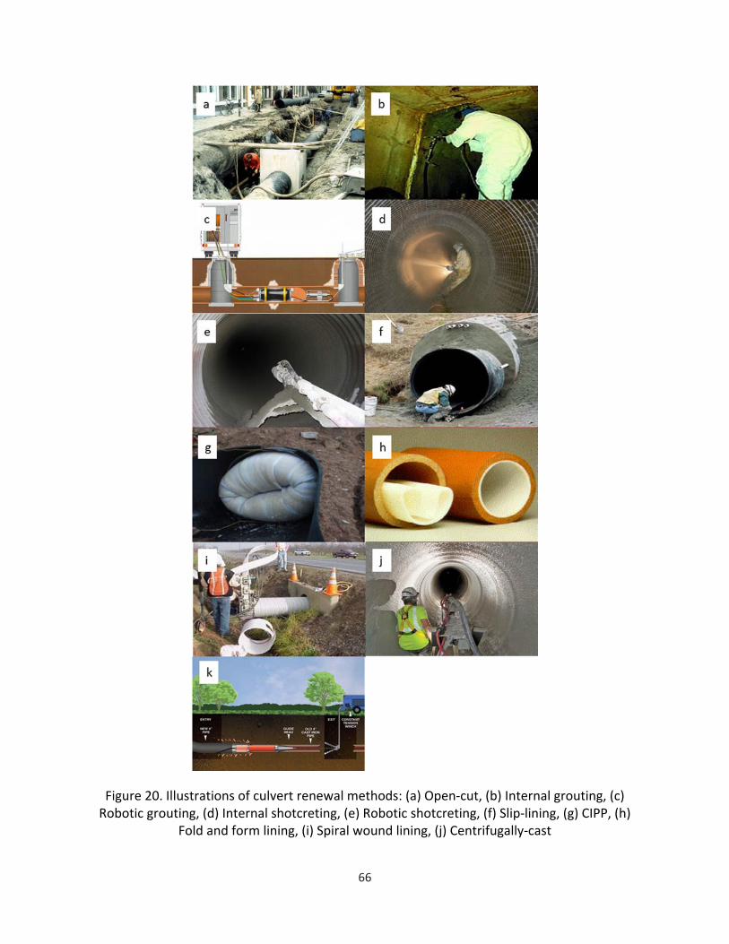
66

Figure 20. Illustrations of culvert renewal methods: (a) Open‐cut, (b) Internal grouting, (c) Robotic grouting, (d) Internal shotcreting, (e) Robotic shotcreting, (f) Slip‐lining, (g) CIPP, (h)

Fold and form lining, (i) Spiral wound lining, (j) Centrifugally‐cast

67

5.2 Evaluation of Culvert Renewal Techniques

Criteria that may influence the decision‐making process of culvert renewal technique selection include but not limited to cost, expected design life, capacity requirements, construction‐related traffic impacts, construction productivity, excavation restrictions, culvert flow level, flow bypassing limitations, safety, culvert access requirements and construction footprint, and environmental impacts. Not all these criteria are relevant in every renewal project. Five criteria, which frequently feature in the decision‐making process (Hunt et al., 2010; Thornton et al., 2005; ProjectMax, 2006; Syachrani et al., 2010; Mitchell et al., 2005), are chosen in this study for comparatively evaluating the culvert renewal techniques; they include cost, expected design life, capacity reduction, traffic impact, and environmental impact.

Table 34. Performance Classes for the Selected Decision Criteria

Cost as considered in this study only indicates the direct cost which includes cost of material, labor and equipment, and excludes costs of societal inconveniences such as traffic delays and detour, noise, air, and water pollution. The cost performance of culvert renewal techniques is synthesized from the literature (Mitchell et al., 2005 and Hunts et al., 2010) and subsequently the techniques are categorized into five different qualitative classes ranging from “High” to “Low” as per the devised scoring convention presented in Table 34.

Expected design life as considered in this study indicates the estimated useful life of the culvert post its renewal. Expected design life varies with the renewal type. Non‐structural renewal, e.g. grouting, may not extend the useful design life of the culvert and therefore expected design life

68

criteria is not crucial for such projects. Similarly, the expected design life varies from semi‐structural to structural renewal type as well. The design life performance of various relevant renewal techniques is synthesized from the literature (Thornton et al., 2005; ProjectMax, 2006; Trenchless Technology Magazine, 2014; Contech Engineered Solutions, 2016; ACPA, 2007; and Rumpca, 1998) and subsequently the techniques are categorized into four quantitative classes ranging from “50 years” to “100 years” as per the devised scoring convention presented in Table 34.

Capacity reduction reflects the ability of a renewal technique to preserve as much culvert flow capacity as possible post its renewal. Renewal techniques are categorized into three qualitative classes namely, “no reduction,” “minor reduction,” and “moderate reduction,” as per the devised scoring convention presented in Table 34.

Traffic impact as considered in this study reflects the potential disturbance to traffic flow caused due to culvert renewal work. Renewal techniques are comparatively evaluated for their potential traffic impact based on the amount of excavation required with each technique. Subsequently, they are categorized into three qualitative classes namely, “low impact,” “moderate impact,” and “severe impact,” as per the devised scoring convention presented in Table 34. For example, if the renewal technique requires minimal to no excavation (possible with CIPP, FFL, SWL), it is considered as “low impact” performance. If the renewal technique requires minimal to reasonable excavation (possibly the case with SL or PB), it is considered as “moderate impact” performance. If a renewal technique requires significant excavation (such as the case with OC), it is considered as “severe impact” performance.

Environmental impact as considered in this study reflects the concerns with the use of certain materials such as mortar or resin which are perceived to be environmentally damaging. Based on the performance of renewal techniques synthesized from literature, they are categorized into three qualitative classes namely, “no impact,” “minor impact,” and “moderate impact,” as per the devised scoring convention presented in Table 34. For example, IG and IS which normally use cement mortar are considered to have minor environmental impact, while RG and RS which normally use chemical grouting are considered to have moderate environmental impact.

Not all the five chosen decision criteria will be relevant in each culvert renewal project. Consequently, decision criteria are appropriately mapped with renewal types (i.e., non‐structural, semi‐structural, and full structural) based on their relevance. For example, cost, expected design life, and environmental impact are considered appropriate for semi‐structural renewal projects, while all five criteria are considered relevant for full‐structural renewal.

The performances of all renewal techniques considered in this study are comparatively evaluated for each of selected criteria based on the literature, as shown in Tables 35‐40. It should be noted that the documented performance data in the literature for the studied renewal techniques was neither entirely quantifiable nor consistent because of which considerable interpretation had to be done with no intentional biases towards any techniques

69

to be able to compare them. Consequently, the comparisons and the subsequent selection preferences should be cautiously used. A more structured comparative objective evaluation of various culvert renewal techniques should be carried out in the future to aid development of more appropriate decision frameworks. As can be observed from Tables 35‐40, the comparative performances are separately synthesized for each renewal type (non‐structural, semi‐structural, and full‐structural) and also for different culvert sizes (<36”, 36~60”, and 60~120”). Only those renewal techniques that can be used for non‐structural, semi‐structural or full structural renewal in each size category are considered for comparative evaluation presented in Tables 35‐40. “Class” scores, which are also presented in Tables 35‐40, are derived based on the performances using the scoring conventions presented in Table 34. Finally, the “ratings,” which are also presented in Tables 35‐40, are derived based on the “class” scores of all renewal techniques using the pair‐wise comparison procedures of analytical hierarchy process (AHP) (Yang, 2011; Najafi and Bhattachar, 2011; and Yoo et al., 2014).


Criteria Category RS CIPP FFL SWL

Cost

Performance Moderate‐High Low Low‐Moderate Low

Class 2 5 4 5

Rating 0.13 0.31 0.25 0.31

Design life

Performance (Years) 50 70* 50* 50

Class 1 1.4 1 1

Rating 0.23 0.31 0.23 0.23

Environmental impact

Performance Moderate Moderate Moderate Minor

Class 1 1 1 2

Rating 0.2 0.2 0.2 0.4 *True performance could be lower than this estimate

Table 36. Evaluation of semi‐structural renewal techniques for 36”‐60”dia. culverts

Criteria Category IS CIPP SWL

Cost

Performance Moderate‐High High High

Class 2 1 1

Rating 0.5 0.25 0.25

Design life

Performance (Years) 50 70* 50

Class 1 1.4 1

Rating 0.29 0.42 0.29


Performance Minor Moderate Minor

Class 2 1 2

Rating 0.4 0.2 0.4 *True performance could be lower than this estimate

70

Table 37. Evaluation of semi‐structural renewal techniques for 60”‐120” dia. culverts

Criteria Category IS SWL

Cost

Performance Moderate‐High High

Class 2 1

Rating 0.67 0.33

Design life

Performance (Years) 50 50

Class 1 1

Rating 0.5 0.5


Performance Minor Minor

Class 2 2

Rating 0.5 0.5

Table 38. Evaluation of full‐structural renewal techniques for <36” dia. culverts

Criteria Category OC SL CIPP SWL PB**

Cost

Performance High Low‐

Moderate Low Low

Low‐Moderate

Class 1 4 5 5 4

Rating 0.06 0.21 0.26 0.26 0.21

Design Life

Performance 75 100* 100* 50 75

Class 1.5 2 2 1 1.5

Rating 0.19 0.25 0.25 0.12 0.19

Capacity Reduction

Performance No Moderate Minor Minor No

Class 3 1 2 2 3

Rating 0.27 0.1 0.18 0.18 0.27

Traffic Impact

Performance Severe Moderate Minor Minor Moderate

Class 1 2 3 3 2

Rating 0.1 0.18 0.27 0.27 0.18

Environmental Impact

Performance No Low Moderate Low No

Class 3 2 1 2 3

Rating 0.27 0.18 0.1 0.18 0.27 *True performance could be lower than this estimate

**Assuming suitable adjustments are made to the bursting technique to make it suitable

71

Table 39. Evaluation of full‐structural renewal techniques for 36”‐60” dia. culverts

Criteria Category OC SL CIPP SWL

Cost

Performance Moderate‐

High Moderate‐

High High High

Class 2 2 1 1

Rating 0.33 0.33 0.17 0.17

Design Life

Performance 75 100* 100* 50

Class 1.5 2 2 1

Rating 0.23 0.31 0.31 0.15

Capacity Reduction

Performance No Moderate Minor Minor

Class 3 1 2 2

Rating 0.38 0.12 0.25 0.25

Traffic Impact

Performance Severe Moderate Minor Minor

Class 1 2 3 3

Rating 0.12 0.22 0.33 0.33


Performance No Low Moderate Low

Class 3 2 1 2


Table 40. Evaluation of full‐structural renewal techniques for 60”‐120” dia. culverts

Criteria Category OC SL SWL

Cost

Performance Moderate to

High High High

Class 2 1 1

Rating 0.5 0.25 0.25

Design Life

Performance 75 100* 50

Class 1.5 2 1

Rating 0.34 0.44 0.22

Capacity Reduction

Performance No Moderate Minor

Class 3 1 2

Rating 0.5 0.17 0.33

Traffic Impact

Performance Severe Moderate Minor

Class 1 2 3

Rating 0.17 0.33 0.5


Performance No Low Low

Class 3 2 2

Rating 0.42 0.29 0.29 *True performance could be lower than this estimate

72

Application scenarios in this study are characterized by culvert material, culvert size, prevalent defect type, and defect severity. Two popular culvert materials are specifically considered, namely reinforced concrete pipe (RCP) and corrugated metal pipe (CMP). Several defects that are commonly observed in culverts include crack (C), invert deterioration (ID), joint misalignment (JM), joint inflow and exfiltration (JI), corrosion (CR), and shape distortion (SD). These defects are further categorized into “minor,” “moderate,” and “major” severity groups. The “minor” type has negligible to insignificant impact on the culvert functionality, while the “moderate” type has reasonable impact on culvert functionality but doesn’t lead to a complete failure of the structure, and the “major” type has significant impact potentially leading to complete failure of the structure in the near future, if left unaddressed. Culverts sizes are categorized into “< 36 inches in diameter (or width),” “≥ 36 inches and < 60 inches,” and “≥ 60 inches and ≤ 120 inches” groups based on the observed transitions in suitability of culvert renewal techniques. For example, RG, RS, PB, and FFL are reported to be only suitable for small sized culverts (< 36 inches in diameter or width), whereas CIPP is also suitable to moderately sized culverts (≥ 36 inches and < 60 inches), IG, IS, and CCCP are suitable for moderate to large sized culverts (≥ 36 inches), and SL and SWL are suitable for a wide range of culvert sizes (up to 120 inches) (Ballinger and Drake, 1995; Caltrans, 2013; Mitchell et al., 2005; Meegoda et al., 2009; Hunt et al., 2010; Hollingshead and Tullis, 2009; and Syachrani et al., 2010). Culverts larger than 120 inch in diameter (or width) may be predominantly renewed using OC and therefore they are deliberately excluded from this study. The classifications highlighted in the previous paragraph are leveraged to develop various typical culvert renewal application scenarios, as shown in Tables 41‐43. The applications scenarios are mapped to appropriate renewal types (i.e., non‐structural, semi‐structural, and full‐structural) based on the structural nature and severity of defects, as shown in Tables 41‐43. Furthermore, the application scenarios are mapped to appropriate renewal techniques that are reported to be suitable, as shown in Tables 41‐43 (Hollingshead and Tullis, 2009; Matthews et al. 2012; Hunt et al., 2010; ProjectMax, 2006; and Syachrani et al., 2010).

5.3 Culvert Renewal Selection Guidance

This section describes an easy‐to‐use, Microsoft Excel‐based decision making tool called Culvert Renewal Selection Tool (CREST) that is developed for the optimal selection of culvert renewal techniques for given application scenarios. The proposed CREST model requires user inputs for the critical decision criteria in the form of percentage weightings that appropriately characterize the relative importance given to the criteria while selecting a renewal technique. The CREST model combines user‐defined percentage weightings and the ratings that are developed in this study (see Tables 35‐40) in order to determine an overall score of each renewal technique for a given application scenario using the principles of Analytical hierarchy process (AHP). AHP is usually employed for simplifying complex decision‐making processes. In AHP, possible alternatives are relatively rated using pair‐wise comparisons based on several decision criteria. The decision criteria are in turn rated using pair‐wise comparisons based on their relative importance to the user. The ratings of the possible alternatives for each criterion are combined with the weightings of the criteria themselves to evaluate the optimal alternative

73

(Saaty, 1987; Saaty, 2008). An overall score (Sj) for each renewal technique (j) is calculated using the following equation: ∑ ∗ , (Eq. 5)

Where, Wi is percentage weighting of criteria i; Ri,j is performance rating of renewal technique j for criteria i; and n is the number of the decision criteria employed.

The overall score (Sj) is the basis for the selection of a renewal technique in the CREST model. Other practical considerations should guide the technique selection in case there is more than one technique with same overall score.

5.4 Demonstration

CREST is demonstrated for all the typical application scenarios developed and presented in Tables 41‐43. The multitude of possibilities in terms of culvert defects, specific field constraints, performance expectations, location constraints, cost limitations, and environmental sensitivities makes it difficult to assign a deterministic set of percentage weightings for the decision criteria that are required as user inputs for the CREST model. For example, cost can be the most decisive criteria in a renewal project when other aspects such as traffic disruption, environmental impacts are inconsequential and no specific field restrictions exist; on the contrary, cost can be a less important criterion in the case of projects with specific requirements or constraints. Given this uncertainty with user preferences of criteria weightings, Monte‐Carlo simulation is employed to randomly generate criteria weightings in 10,000 simulations for each application scenario using uniform probability distribution. The optimal renewal technique in each simulation is identified based on the best overall score (Sj) calculated using CREST.

5.4.1 Results and Discussion The findings resulted from the demonstration of the CREST are appropriately grouped in this section based on the application scenarios each renewal technique is found to be best suitable for. Application scenarios are characterized by culvert material (i.e., RCP or CMP), culvert size (which includes <36”, 36”‐60”, and 60”‐120”), defect types (including crack, corrosion, joint in/exfiltration, joint misalignment, invert deterioration, and shape deformation), and severity (including minor, moderate, and major). The results are presented separately for RCP and CMP application scenarios. The results indicate the percentage of 10,000 Monte‐Carlo simulations in which each renewal technique is found to be best suited for a given application scenario. The ranges of criteria weightings that are found to drive the selection of renewal techniques for each application scenario are subsequently identified and discussed.

74

Table 41. Mapping of RCP application scenarios to renewal types and techniques for <36” dia. culverts

Application Scenarios Culvert Renewal Techniques

Percentage Preference Size Defect types Severity Renewal Type

<36"

Crack

Minor NS RG 100%

Moderate NS RG 100%

SS CIPP 100%

Major

SS CIPP 100%

FFL 0%

FS

SL 1%

CIPP 50.8%

PB 48.2%

OC 0%

JM

Moderate SS CIPP 100%

FFL 0%

Major FS PB 100%

OC 0%

JI

Minor NS RG 100%

Moderate

NS RG 100%

SS

CIPP 31.6%

FFL 0%

SWL 68.4%

Major

SS

CIPP 31.6%

FFL 0%

SWL 68.4%

FS

CIPP 43%

SWL 13.4%

PB 43.6%

OC 0%

ID

Minor NS RS 100%

moderate

NS RS 100%

SS RS 0%

SWL 100%

Major FS

SL 3%

CIPP 51.4%

SWL 25.6%

OC 20% Note: FFL can only be used for circular culverts; NS: Non‐Structural; SS: Semi‐Structural; FF: Full‐Structural

75


dia. culverts



36"~60"

Crack

Minor NS IG 100%

Moderate NS IG 100%

SS CIPP 100%

Major

SS CIPP 100%

FS

SL 16.3%

CIPP 29.7%

OC 54%

JM Moderate SS CIPP 100%

Major FS OC 100%

JI

Minor NS IG 100%

Moderate

NS IG 100%

SS CIPP 37.3%

SWL 62.7%

Major

SS CIPP 37.3%

SWL 62.7%

FS

SL 15.6%

CIPP 24.2%

SWL 9.8%

OC 50.4%

ID

Minor NS IS 100%

Moderate

NS IS 100%

SS IS 100%

SWL 0%

Major FS

SL 15.6%

CIPP 24.2%

SWL 9.8%

OC 50.4%

Note: NS: Non‐Structural; SS: Semi‐Structural; FF: Full‐Structural

76

Table 43. Mapping of RCP application scenarios to renewal types and techniques for 60”‐120” dia. culverts



60"~120"

Crack

Minor NS IG 100%

Moderate NS IG 100%

SS SWL 100%

Major

SS SWL 100%

FS SL 24.8%

OC 75.2%

JM

Moderate SS SWL 100%

Major SS SWL 100%

FS OC 100%

JI

Minor NS IG 100%

Moderate NS IG 100%

SS SWL 100%

Major

SS SWL 100%

FS

SL 10%

SWL 28.5%

OC 61.5%

ID

Minor NS IS 100%

Moderate

NS IS 100%

SS IS 100%

SWL 0%

Major FS

SL 10%

SWL 28.5%

OC 61.5%

Note: NS: Non‐Structural; SS: Semi‐Structural; FF: Full‐Structural

77

Table 44. Range of criteria weightings for semi‐ and full‐ structural culvert renewal techniques for RCP culverts

Structural Types

Application Scenarios

Suitable Renewal

Techniques

Percentage Preference

Suitable Ranges of Criteria Weightings

Cost Design

life Environmental

Impact Capacity

Reduction Traffic Impact

Semi- Structural

JI <36, Moderate-Major CIPP 31.6% - 50-100% 0-20%

N/A SWL 68.4% 0-100% 0-50% 20-100%

JI 36-60, Moderate-Major CIPP 37.3% 50-100% 0-20% SWL 62.7% 0-100% 0-50% 20-100%

Full- Structural

Crack <36”, Major SL 1% - - - - -

CIPP 50.8% 10-100% 10-100% 0-10% 0-20% 20-100% PB 48.2% 0-20% 0-20% 10-100% 20-100% 0-30%

JI <36, Major CIPP 43% 20-100% 10-100% 0-10% 0-20% 30-100% SWL 13.4% - - - - - PB 43.6% 0-20% 0-20% 10-100% 20-100% 0-30%

ID <36, Major

SL 3% - - - - - CIPP 51.4% 0-100% 10-100% 0-20% 0-50% 0-100% SWL 25.6% 0-10% 20-40% OC 20% 40-100% 50-100%

Crack 36-60, Major

SL 16.3% 50-100% 50-80% CIPP 29.7% 30-100% 0-10% 30-100% OC 54% 0-80% 0-30% 10-100% 0-100% 0-30%

JI 36-60, Major

ID 36-60, Major

SL 15.6% 60-100% 70-80% CIPP 24.2% 30-100% 0-10% 30-100% SWL 9.8% - - - - - OC 50.4% 0-80% 0-30% 10-100% 0-100% 0-30%

Crack 60-120, Major SL 24.8% 40-100% 40-100% OC 75.2% 0-100% 0-40% 0-100% 0-100% 0-50%

JI 60-120, Major

ID 60-120, Major

SL 10% 40-100% SWL 28.5% 30-100% OC 61.5% 0-100% 0-40% 0-100% 0-100% 0-30%

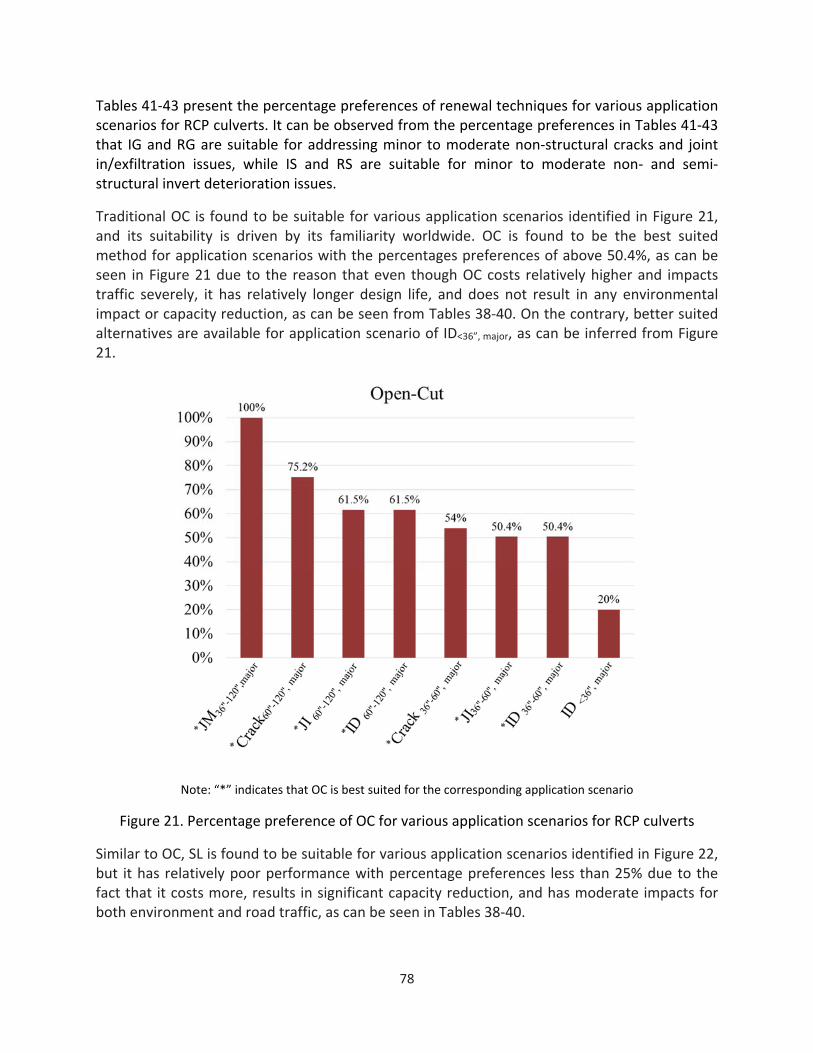
78

Tables 41‐43 present the percentage preferences of renewal techniques for various application scenarios for RCP culverts. It can be observed from the percentage preferences in Tables 41‐43 that IG and RG are suitable for addressing minor to moderate non‐structural cracks and joint in/exfiltration issues, while IS and RS are suitable for minor to moderate non‐ and semi‐structural invert deterioration issues.

Traditional OC is found to be suitable for various application scenarios identified in Figure 21, and its suitability is driven by its familiarity worldwide. OC is found to be the best suited method for application scenarios with the percentages preferences of above 50.4%, as can be seen in Figure 21 due to the reason that even though OC costs relatively higher and impacts traffic severely, it has relatively longer design life, and does not result in any environmental impact or capacity reduction, as can be seen from Tables 38‐40. On the contrary, better suited alternatives are available for application scenario of ID<36”, major, as can be inferred from Figure 21.

Note: “*” indicates that OC is best suited for the corresponding application scenario

Figure 21. Percentage preference of OC for various application scenarios for RCP culverts

Similar to OC, SL is found to be suitable for various application scenarios identified in Figure 22, but it has relatively poor performance with percentage preferences less than 25% due to the fact that it costs more, results in significant capacity reduction, and has moderate impacts for both environment and road traffic, as can be seen in Tables 38‐40.

79

Figure 22. Percentage preference of SL for various application scenarios for RCP culverts

CIPP is found to be suitable for various application scenarios as can be seen in Figures 23 (semi‐structural) and 24 (full‐structural), and this is mainly due to its broader application range in terms of host pipe material, size, shape, and its flexibility to be used as a structural or semi‐structural liner (Ballinger and Drake, 1995; Caltrans, 2013; Mitchell et al., 2005; Meegoda et al., 2009; Hunt et al., 2010; Hollingshead and Tullis, 2009; Syachrani et al., 2010; and Yazdekhasti et al., 2014). However, it has been selected as the best choice for only three application scenarios while for most of the other application scenarios it is selected with lower percentage preference as can be seen in Figures 23 and 24. The reason is due to the fact that it has more environmental impact compared to SWL (SS), PB, and OC as shown in Tables 35 and 36. Furthermore, CIPP (FS) has more capacity reduction compared to PB and OC as can be seen in Tables 38 and 39.

80

Note: “*” indicates that CIPP (semi‐structural) is best suited for the corresponding application scenario

Figure 23. Percentage preference of CIPP (semi‐structural) for various application scenarios for RCP culverts

Note: “*” indicates that CIPP (full‐structural) is best suited for the corresponding application scenario

Figure 24. Percentage preference of CIPP (full‐structural) for various application scenarios for RCP culverts

SWL is found to be best suited for all application scenarios with percentage preference of above 60% for semi‐structural renewal identified in Figure 25, while that of full‐structural renewal is found to be not selected as any best choice with the percentage preferences of less than 30% as can be seen in Figure 26. The main reason is that SWL in case of semi‐structural renewal has

81

minor environmental impact compared to CIPP as can be seen from Tables 35 and 36, while that of full‐structural renewal has relatively shorter design life and costs more for sizes of 36‐60 inches’ culverts as can be seen in Tables 38 and 39.

Note: “*” indicates that SWL (semi‐structural) is best suited for the corresponding application scenario

Figure 25. Percentage preference of SWL (semi‐structural) for various application scenarios for RCP culverts

82

Figure 26. Percentage preference of SWL (full‐structural) for various application scenarios for RCP culverts

PB has been selected to address only three application scenarios due to its limited application range in terms of host pipe material and size. However, it is found to be suited with higher percentage preference of above 40% as can be seen in Figure 27 due to the reason that it has relatively higher cost and design life and no environmental impact and capacity reduction as shown in Table 38. It should be noted that the traditional pipe bursting method may need to be adjusted to be suitable for both RCP.

Note: “*” indicates that PB is best suited for the corresponding application scenario

Figure 27. Percentage preference of PB for various application scenarios for RCP culverts

83

FFL has not been selected during demonstrating scenarios due to its higher cost and shorter design life compared to CIPP as shown in Table 35. However, FFL may be preferred in situations where negligible reduction in culvert capacity is desired.

Furthermore, the ranges of criteria weightings that are found to drive the selection of renewal techniques for each application scenario are subsequently identified and discussed as shown in Table 44. For example, it can be observed from Table 44 that CIPP (semi‐structural) is most likely the best choice when criteria weighting for expected design life is in the range of 50‐100% and environmental impact in the range of 0‐20% for addressing JI <36, Moderate‐Major defects, whereas SWL (semi‐structural) is best suited when criteria weighting for cost is in the range of 0~100%, design life in the range of 0~50%, and environmental impact in the rage of 20~100%.

Tables 45‐50 present the comparative evaluation of various semi‐structural and full structural renewal techniques for CMP culverts. Similar to the results of the RCP application scenarios, Tables 51‐53 present the results – in terms of percentage preferences of various renewal techniques in each application scenario – for CMP application scenarios. Tables 54‐56 present the ranges of criteria weightings that will result in the selection of a given renewal technique. Also, Figures 28‐35 illustrate the preference of several renewal techniques for various CMP application scenarios.

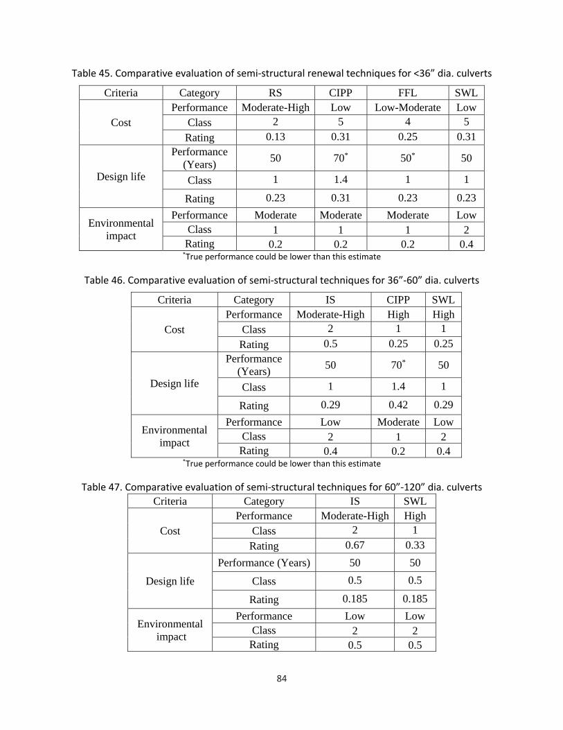
84


Criteria Category RS CIPP FFL SWL

Cost Performance Moderate-High Low Low-Moderate Low

Class 2 5 4 5

Rating 0.13 0.31 0.25 0.31

Design life

Performance (Years)

50 70* 50* 50

Class 1 1.4 1 1

Rating 0.23 0.31 0.23 0.23


Performance Moderate Moderate Moderate Low Class 1 1 1 2 Rating 0.2 0.2 0.2 0.4 *True performance could be lower than this estimate

Table 46. Comparative evaluation of semi‐structural techniques for 36”‐60” dia. culverts

Criteria Category IS CIPP SWL

Cost Performance Moderate-High High High

Class 2 1 1

Rating 0.5 0.25 0.25

Design life

Performance (Years)

50 70* 50

Class 1 1.4 1

Rating 0.29 0.42 0.29


Performance Low Moderate Low Class 2 1 2 Rating 0.4 0.2 0.4

*True performance could be lower than this estimate

Table 47. Comparative evaluation of semi‐structural techniques for 60”‐120” dia. culverts

Criteria Category IS SWL

Cost Performance Moderate-High High

Class 2 1

Rating 0.67 0.33

Design life

Performance (Years) 50 50

Class 0.5 0.5

Rating 0.185 0.185


Performance Low Low Class 2 2 Rating 0.5 0.5

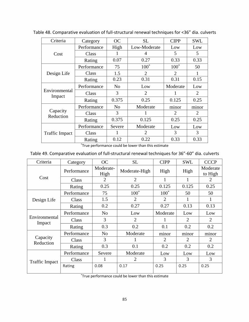
85

Table 48. Comparative evaluation of full‐structural renewal techniques for <36” dia. culverts

Criteria Category OC SL CIPP SWL

Cost Performance High Low-Moderate Low Low

Class 1 4 5 5

Rating 0.07 0.27 0.33 0.33

Design Life Performance 75 100* 100* 50

Class 1.5 2 2 1 Rating 0.23 0.31 0.31 0.15


Performance No Low Moderate Low

Class 3 2 1 2

Rating 0.375 0.25 0.125 0.25

Capacity Reduction

Performance No Moderate minor minor Class 3 1 2 2

Rating 0.375 0.125 0.25 0.25

Traffic Impact Performance Severe Moderate Low Low

Class 1 2 3 3


Table 49. Comparative evaluation of full‐structural renewal techniques for 36”‐60” dia. culverts

Criteria Category OC SL CIPP SWL CCCP

Cost Performance

Moderate-High

Moderate-High High High Moderate to High

Class 2 2 1 1 2

Rating 0.25 0.25 0.125 0.125 0.25

Design Life Performance 75 100* 100* 50 50

Class 1.5 2 2 1 1

Rating 0.2 0.27 0.27 0.13 0.13


Performance No Low Moderate Low Low

Class 3 2 1 2 2

Rating 0.3 0.2 0.1 0.2 0.2

Capacity Reduction

Performance No Moderate minor minor minor Class 3 1 2 2 2

Rating 0.3 0.1 0.2 0.2 0.2

Traffic Impact

Performance Severe Moderate Low Low Low Class 1 2 3 3 3

Rating 0.08 0.17 0.25 0.25 0.25

*True performance could be lower than this estimate

86

Table 50. Comparative evaluation of full‐structural renewal techniques for 60”‐120” dia. culverts

Criteria Category OC SL SWL CCCP

Cost Performance

Moderate-High

High High Moderate to High

Class 2 1 1 2

Rating 0.33 0.17 0.17 0.33

Design Life Performance 75 100* 50 50

Class 1.5 2 1 1

Rating 0.27 0.37 0.18 0.18


Performance No Low Low Low

Class 3 2 2 2

Rating 0.34 0.22 0.22 0.22

Capacity Reduction

Performance No Moderate minor minor Class 3 1 2 2

Rating 0.375 0.125 0.25 0.25

Traffic Impact Performance Severe Moderate Low Low

Class 1 2 3 3


87

Table 51. Mapping of CMP application scenarios to renewal types and techniques for <36” dia. culverts

Application Scenarios Culvert Renewal

Techniques Percentage Preference Size Defect types Severity

Renewal Type

<36"

Joint misalignment Moderate SS

CIPP 100% FFL 0%

Major FS OC 100%

Corrosion

Minor NS RS 100%

Moderate NS RS 100%

SS RS 0%

CIPP 100%

Major

SS RS 0%

CIPP 31.6% SWL 68.4%

FS

SL 4.3% CIPP 43% SWL 26.2% OC 26.5%

Joint in/exfiltration

Minor NS RG 100%

Moderate NS RG 100% SS CIPP 100%

Major

SS CIPP 31.6% FFL 0% SWL 68.4%

FS

SL 4.3% CIPP 43% SWL 26.2% OC 26.5%


Minor NS RS 100%

Moderate NS RS 100%

SS RS 0%

CIPP 100%

Major FS SL 6.4%

CIPP 63.6% OC 30%

Shape deformation Moderate SS

CIPP 100% FFL 0%

Major FS SL 57.5% OC 42.5%

Note: FFL is only used for circular culverts; NS: Non-Structural; SS: Semi-Structural; FF: Full-Structural

88

Table 52. Mapping of CMP application scenarios to renewal types and techniques for 36”‐60” dia. culverts



Renewal Type

36"~60"

Joint misalignment Moderate SS CIPP 100%

Major FS OC 100%

Corrosion

Minor NS IS 100% Moderate NS, SS IS 100%

Major

SS IS 87.8%

CIPP 12.2% SWL 0%

FS

SL 11.5% CIPP 14% SWL 3% CCCP 16.5%

OC 55%


Minor NS IG 100%

Moderate NS IG 100% SS CIPP 100%

Major

SS CIPP 37.3% SWL 62.7%

FS

SL 11.5% CIPP 14% SWL 3% CCCP 16.5%

OC 55%



Major FS SL 17%

CCCP 26% OC 57%

Shape deformation

Moderate SS CIPP 100%

Major FS SL 16.2%

CIPP 22.2% OC 61.6%

Note: FFL is applicable only in round shape culvert; NS: Non‐Structural; SS: Semi‐Structural; FF: Full‐

Structural

89

Table 53. Mapping of CMP application scenarios to renewal types and techniques for 60”‐120” dia. culverts



Renewal Type

60"~120"

Joint misalignment Moderate SS SWL 100%

Major SS SWL 100% FS OC 100%

Corrosion


Major

SS IS 100%

SWL 0%

FS

SL 10% SWL 6.5% CCCP 23.5%

OC 60%


Minor NS IG 100%

Moderate NS IG 100% SS SWL 100%

Major

SS SWL 100%

FS

SL 10% SWL 6.5% CCCP 23.5%

OC 60%


Minor NS IS 100%

Moderate NS, SS IS 100%

Major FS SL 10%

CCCP 30% OC 60%

Shape deformation Moderate SS SWL 100%

Major FS SL 20.3% OC 79.7%

Note: FFL is applicable only in round shape culvert; NS: Non‐Structural; SS: Semi‐Structural; FF: Full‐

Structural

90

Table 54. Range of criteria weightings for semi‐structural CMP culvert renewal techniques


Suitable Renewal Techniques


Suitable Ranges of Criteria Weightings Cost Design life Environmental Impact

JI <36, Major CIPP 31.6% - 50-100% 0-20% SWL 68.4% 0-100% 0-50% 20-100%

Corrosion <36, Major CIPP 31.6% - 50-100% 0-20% SWL 68.4% 0-100% 0-50% 20-100%

JI 36-60, Major CIPP 37.3% 50-100% 0-20% SWL 62.7% 0-100% 0-50% 20-100%

Corrosion 36-60, Major IS 87.8% 0-100% 0-70% 0-100%

CIPP 12.2% - 70-100% -

91

Table 55. Range of criteria weightings for full‐structural CMP culvert renewal techniques of sizes <36 inches diameter


Suitable Renewal

Techniques



Cost Design life Environmental

Impact Capacity


Corrosion <36, Major

JI <36, Major

SL 4.3% - - - - - CIPP 43% 10-100% 10-100% 0-20% 0-40% 10-100% SWL 26.2% 60-90% 0-10% 20-40% - - OC 26.5% 0-10% - 40-100% 40-100% 0-10%

ID <36, Major SL 6.4% - - - - -

CIPP 63.6% 0-100% 0-100% 0-30% 0-50% 10-100% OC 30% - - 30-100% 50-100% 0-10%

SD <36, Major SL 57.5% 20-100% 0-10%, 20-100% 0-40% 0-30% 10-100% OC 42.5% 0-20% 10-20% 30-100% 30-100% 0-10%

92

Table 56. Range of criteria weightings for full‐structural culvert renewal techniques of sizes 36”‐120” diameter

Application Scenarios Suitable Renewal

Techniques



Cost Design life Environmental

Impact Capacity


SD 36-60, Major SL 16.2% - 50-100% - -

CIPP 22.2% - 70-920% - - 40-100% OC 61.6% 0-100% 0-50% 0-100% 0-100% 0-40%

Corrosion 36-60, Major

JI 36-60, Major

SL 11.5% - 50-90% - - - CIPP 14% - 80-90% - - 70-100% SWL 3% - - - - - CCCP 16.5% - 10-20% - - 30-80%

OC 55% 0-100% 0-10%, 20-50% 0-100% 0-100% 0-30%

ID 36-60, Major

SL 17% - 60-100% - - - CCCP 26% - - - - 30-100%

OC 57% 0-100% 0-60% 0-100% 0-100% 0-30%

Corrosion 60-120, Major

JI 60-120, Major

SL 10% - 60-100% - - SWL 6.5% - - - - 70-100% CCCP 23.5% - - - - 30-80%

OC 60% 0-100% 0-60% 0-100% 0-100% 0-30%

ID 60-120, Major

SL 10% - 60-100% - - - CCCP 30% 90-100% - - - 30-100%

OC 60% 0-100% 0-60% 0-100% 0-100% 0-30%

SD 60-120, Major SL 20.3% - 60-100% - - 50-100% OC 79.7% 0-100% 0-60% 0-100% 0-100% 0-50%

93

Note: “*” indicates that OC is best suited for the corresponding application scenario

Figure 28. Percentage preference of OC for various application scenarios for CMP culverts

94

Note: “*” indicates that IS is best suited for the corresponding application scenario

Figure 29. Percentage preference of IS for various application scenarios for CMP culverts

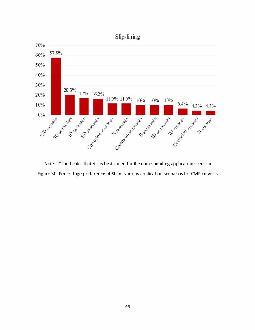
95

Note: “*” indicates that SL is best suited for the corresponding application scenario

Figure 30. Percentage preference of SL for various application scenarios for CMP culverts

96

Note: “*” indicates that CIPP (semi-structural) is best suited for the corresponding application scenario

Figure 31. Percentage preference of CIPP (semi‐structural) for various application scenarios for CMP culverts

97

Note: “*” indicates that CIPP (full-structural) is best suited for the corresponding application scenario

Figure 32. Percentage preference of CIPP (full‐structural) for various application scenarios for CMP culverts

98

Note: “*” indicates that SWL (semi-structural) is best suited for the corresponding application scenario

Figure 33. Percentage preference of SWL (semi‐structural) for various application scenarios for CMP culverts

99

Note: “*” indicates that SWL (full-structural) is best suited for the corresponding application scenario

Figure 34. Percentage preference of SWL (full‐structural) for various application scenarios for CMP culverts

100

Note: “*” indicates that CCCP is best suited for the corresponding application scenario

Figure 35. Percentage preference of CCCP for various application scenarios for CMP culverts

5.4 Validation of the CREST Model

In order to strengthen the findings of the CREST model presented in the previous section, this section describes the validation effort undertaken and summarizes the results of the same. Validation is a scientific process used to confirm that the research approach is indeed suitable for meeting the desired objectives. In the context of this study, validation measures the capability of the proposed analytical model to truly predict the desired outcome in terms of optimal selection of culvert renewal techniques. A validated tool or model can be used to judge the quality, reliability, and consistency of analytical results (Ludwig Huber, 1998). Validation techniques are usually different for quantitative and qualitative research studies (Golafshani, 2003). There is less clarity on the need and appropriateness of various validation techniques for qualitative studies and it is suggested to be affected by the researcher’s perception of validity (Creswell and Miller, 2000). As a result, several previous researchers have themselves devised validation techniques that they considered appropriate (Davies and Dodd, 2002; Lincoln and Guba, 1985; Seale, 1999; and Stenbacka, 2001).

A novel approach, called practice‐based reflective validation (PRV), has been devised and employed in this quasi‐qualitative study to validate both CREST and the resulting findings presented in Chapter 5. In the PRV approach, expert knowledge for determining culvert renewal method selection preferences in real world is tapped. Several design consultants (or

101

experts) work closely with culvert asset managers to thoroughly understand each culvert renewal scenario and subsequently evaluate the most suitable technique that meets the preferences (i.e., in terms of budget, traffic impacts, and etc.) of the owners. The assumptions made in this kind of validation method are that the expert decisions are rational and unbiased. Instead of surveying these experts, which could be a time consuming procedure and may also result in insignificant response rate, various real‐world, documented culvert renewal case studies are reviewed. The rationale is that the expertise of design consultants is embedded in the selection preferences of real‐world culvert renewal projects and therefore, these case studies will serve as a good measure of the validity of CREST. Twenty six real‐world case studies are reviewed to employ the PRV approach. The twenty six cases captured a wide range of application scenarios as shown in Table 57. All these cases involved either RCP or CMP culverts which are the most concerning culvert materials to transportation agencies. These case studies are collected from both consultants’ and contractors’ websites. To ensure the reliability of the validation, it is ideal to obtain data from consultants/contractors that are capable of using several of the studied renewal methods; however, there were few contractors that are experienced in multiple trenchless renewal techniques. Consequently, data is obtained from consultants/contractors who are experienced with as many renewal techniques as possible. The actual renewal technique selected in each of the 26 cases is compared to the predicted technique from CREST, as shown in Tables 58 and 59.

Twenty‐two (85%) out of the 26 documented projects are from 12 different states in the U.S., whereas the remaining five (15%) are from other countries. The information gathered for each project includes year of renewal, asset owner, contractor, culvert material, shape, size, length, major defect, and selected renewal technique. Appendix D presents all these details for all the 26 case studies.

A validation measure called validation score is defined and used in the proposed PRV approach to quantify the comparison of the predicted and actual renewal technique selections in each of the 26 case studies. The validation score (VSj) is calculated using Eq. 6.

,

∈ , (Eq. 6)

Where, VSj is validation score for application scenario j, PPi,j is the percentage preference of the actual renewal technique i as per CREST for application scenario j; n is the number of renewal techniques considered to be suitable for a given application scenario j.

CREST has been used to estimate selection preferences of various suitable culvert renewal methods to each of the 26 project scenarios documented. The validation score will be one when the best suited renewal method as per CREST is same as the actual renewal technique used in a given project. The validation score will proportionately diminish if the predicted best suitable method is different from the actual renewal method. The comparison of the actual renewal technique selected and the predicted preferences of various suitable renewal methods are presented in Table 58 for RCP culvert projects and in Table 59 for CMP projects. As can be observed from Tables 58 and 59, the actual renewal method selected and the predicted best

102

suitable method (as per CREST) is the same in 13 out of the 26 cases (or 50% of the cases) resulting in a validation score of 1. It can be further observed from Tables 58 and 59 that the actual renewal method is the second best suitable method as per CREST in four more cases resulting in a validation score 0.89. Similarly, validation scores in Tables 58 and 59 for all the other cases can be interpreted. The mean and median validation scores for the 26 case studies synthesized are 0.8 and 0.95 respectively, which highlights the merit of CREST and the findings of this study.

It is understandable that in a few cases, the actual technique selections are different from the predicted techniques which are derived for average application scenarios. It can be observed from the comparison presented in Tables 58 and 59 that SWL method has been used in a few projects where SL was found to be best suitable as per CREST. Case study #2 is an example for such disparity. In case study #2, the culvert in Lakehurst Naval Air Station, NJ has deteriorated to an extent where it is no longer hydraulically or structurally adequate. Without considering any other constraints in this project, it seems that SL would be suitable and it has even been determined by CREST as the best choice. In reality however, this project had tight space constraints which probably made the project team go with SPR™ PE technique, a type of SWL method, that enabled the project team re‐line the culvert by accessing it through the manhole structure (Contech, 2014a). Similarly, other disparities observed in this validation effort can be attributed to the unique project constraints that are difficult to generalize.

103

Table 57. Selected culvert defects and case studies for validation

Material Major defect # of Case studies

RCP Crack 2

Invert deterioration 5 Multiple defects 3

CMP

Corrosion 10 Invert deterioration 2

Joint separation 1 Multiple defects 3

104

Table 58. Validation of findings for RCP applications

Case Year Shape Size (in)

Length (ft)

Major defect

Actual technique selection

References Predicted choice

Validation score

1 Unknown Circular 24 18 Crack SL Contech, 2016 SL: 38%

CIPP: 33.8% FFL: 28.2%

1

2 2014 Circular 48 786 ID SWL Contech, 2014a

SL: 38% CIPP: 33.8% CCCP: 27.7% SWL: 0.5%

0.013

3 2014 Circular 54 703 ID SWL Contech, 2014a 0.013

4 2012 Circular 54 300 Crack SL Contech, 2012a 1

5 2010 Circular 96 500 ID SL Contech, 2010 1

6 2012 Box 120 80 ID SL Contech, 2012b 1

7 2013 Circular 144 360*2 ID SL Contech, 2013 1

8 2012 Circular 72 Unknown Multiple SL Contech, 2012c 1

9 2014 Circular 96 42 Multiple SL Contech, 2014b 1

10 2014 Circular 120 1500 Multiple SL Contech, 2014c 1

105

Table 59. Validation of findings for CMP applications

Case Year Shape Size (in)

Length (ft)

Major defect


References Predicted choice

Validation score

11 2010 Circular 36 160 Corrosion CIPP Insituform, 2010

SL: 38% CIPP:33.8% CCCP:27.7% SWL: 0.5%

0.89

12 2010 Circular 36 160 Corrosion CIPP Insituform, 2010 0.89

13 2010 Circular 36 80 Corrosion CCCP MDOT, 2012 0.73

14 2013 Circular 45 550 Corrosion SWL MDOT, 2012 0.013



17 Unknown Circular 60 220 Corrosion CCCP Milliken, 2015a 0.73

18 2013 Circular 66 25 Corrosion CCCP Milliken, 2013 0.73

19 2015 Circular 132 106 Corrosion SL Contech, 2015a 1

20 2014 Circular 74 38*2 ID SL Contech, 2014e 1

21 2014 Ellipse 72 2208 ID SL Contech, 2015b 1

22 Unknown Circular 66 130 Multiple CCCP Milliken, 2015c 0.73

23 Unknown Arch 72 700 Multiple CCCP Milliken, 2015d SL: 59.4%, CCCP:40.6%,

0.68

24 2012 Circular 120 86 Multiple SL Contech, 2012d 1

25 2013 Circular 18~36 6000 Corrosion SL Contech, 2014d

SL: 44% CIPP: 38.1% SWL: 16.9% RS: 1.1%

1

26 Unknown Circular 120 300 JI CCCP Milliken, 2015b SL: 59.4%,

CCCP:39.3%, SWL: 1.3%

0.66

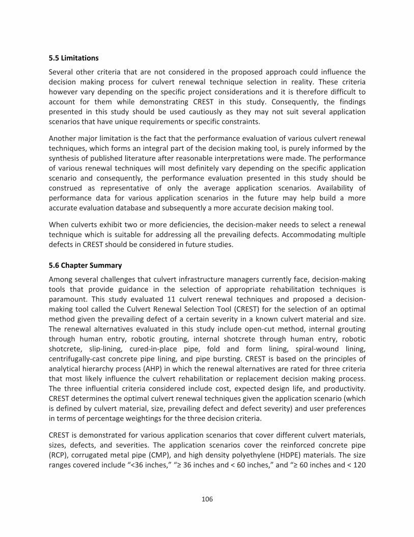
106

5.5 Limitations

Several other criteria that are not considered in the proposed approach could influence the decision making process for culvert renewal technique selection in reality. These criteria however vary depending on the specific project considerations and it is therefore difficult to account for them while demonstrating CREST in this study. Consequently, the findings presented in this study should be used cautiously as they may not suit several application scenarios that have unique requirements or specific constraints.

Another major limitation is the fact that the performance evaluation of various culvert renewal techniques, which forms an integral part of the decision making tool, is purely informed by the synthesis of published literature after reasonable interpretations were made. The performance of various renewal techniques will most definitely vary depending on the specific application scenario and consequently, the performance evaluation presented in this study should be construed as representative of only the average application scenarios. Availability of performance data for various application scenarios in the future may help build a more accurate evaluation database and subsequently a more accurate decision making tool.

When culverts exhibit two or more deficiencies, the decision‐maker needs to select a renewal technique which is suitable for addressing all the prevailing defects. Accommodating multiple defects in CREST should be considered in future studies.

5.6 Chapter Summary

Among several challenges that culvert infrastructure managers currently face, decision‐making tools that provide guidance in the selection of appropriate rehabilitation techniques is paramount. This study evaluated 11 culvert renewal techniques and proposed a decision‐making tool called the Culvert Renewal Selection Tool (CREST) for the selection of an optimal method given the prevailing defect of a certain severity in a known culvert material and size. The renewal alternatives evaluated in this study include open‐cut method, internal grouting through human entry, robotic grouting, internal shotcrete through human entry, robotic shotcrete, slip‐lining, cured‐in‐place pipe, fold and form lining, spiral‐wound lining, centrifugally‐cast concrete pipe lining, and pipe bursting. CREST is based on the principles of analytical hierarchy process (AHP) in which the renewal alternatives are rated for three criteria that most likely influence the culvert rehabilitation or replacement decision making process. The three influential criteria considered include cost, expected design life, and productivity. CREST determines the optimal culvert renewal techniques given the application scenario (which is defined by culvert material, size, prevailing defect and defect severity) and user preferences in terms of percentage weightings for the three decision criteria.

CREST is demonstrated for various application scenarios that cover different culvert materials, sizes, defects, and severities. The application scenarios cover the reinforced concrete pipe (RCP), corrugated metal pipe (CMP), and high density polyethylene (HDPE) materials. The size ranges covered include “<36 inches,” “≥ 36 inches and < 60 inches,” and “≥ 60 inches and < 120

107

inches.” Various defects that are commonly observed in RCP, CMP and HDPE culverts are covered by categorizing their severities into “minor,” “moderate,” and “severe.”

108

6. CONCLUSIONS AND RECOMMENDATIONS

6.1 Major Outcomes and Limitations of the Research

Major outcomes and limitations of this research study are broadly classified into three categories:

6.1.1 Predicting Future Condition of Culvert Structures

Two types of deterioration models were developed that mapped a variety of physical (e.g., culvert material, size, shape, and etc.) and environmental (e.g., pH, runoff coefficient, temperature, and precipitation) input variables with the evaluation (as in model outputs) scores present in the SCDOT’s culvert inventory database. The first type of deterioration models are artificial neural networks (ANNs), while the second type are logistic regression‐based. ANNs were found to be reasonably promising for predicting the output scores of a certain type of culverts, while logistic regression proved promising for others. Overall, four input variables were to be significant; they include: pH, runoff coefficient, temperature, and precipitation.

While these deterioration models could potentially be useful in predicting the future condition of SCDOT’s culvert infrastructure without even inspecting them, there are certain limitations that may dimnish their accuracy. Significant limitations include: (a) the spatial bias that arised due to the linear interpoloation of several environmental input variables based on the latitude and longitude data in the SCDOT’s culvert inventory database. In other words, closely located culverts with similar physical characteristics will result in similar output scores, thereby missing to capture possible inherent variations; and (b) the lack of a time‐dependent input variable in both the types of deterioration models prevents the accounting of age‐based deterioration of culverts. In other words, predicted output variables for similar environmental characteristics would be approximately same irrespective of whether it is a brand new culvert or a 60‐year old culvert.

6.1.2 Identifying and Prioritizing Risky Culverts

A failure risk‐based prioritization model has been developed to rank the culverts in the decreasing order of their failure risk. Only barrel’s failure risk is considered in this study to develop the model and demonstrate it. Failure risk is defined as the product of criticality and estimated failure consequences. Criticality of the culvert barrel is estimated using the principles of analytical hierarchy process (AHP), i.e. through a combination of assessment scores in the SCDOT’s culvert inventory database and defect weightings obtained from the survey of other state DOTs. The barrel defects included in the failure risk analysis of RCP culverts include crack, joint Misalignment, joint inflow/infiltration, bedding Voids, and invert deterioration, while those of CMP culverts include corrosion, joint misalignment, shape distortion, joint inflow/infiltration, bedding voids, and invert deterioration. The failure risk‐based prioritization model was demonstrated on sets of RCP and CMP culverts that were assessed and reported in the SCDOT’s culvert inventory database.

109

It was determined that about 61.3% of RCP culverts (only those recorded in SCDOT’s inventory database) measured by length (≈ 55.1 miles) were at no risk, while about about 4% (≈ 1.42 miles) were found to be somewhat risky. Similarly, about 39% of CMP culverts (≈1.7 miles) were determined to be no risk, while about 13% (≈0.4 miles) are found to be somewhat risky. The failure risk assessment approach demonstrated in this project does have some limitations which include: (a) the limited number of survey responses (only 8 completed) that informed the defect‐weightings derived in this study; (b) the lack of consideration of inlet and outlet structures as part of the failure risk assessment is another limitation that may be addressed in the future; (c) the uncertainty with respect to the consistency with which defect scoring is carried out, especially when multiple inspectors are engaged. While these limitations should be looked into in the future, SCDOT can easily modify the defect weightings and the failure consequence estimates in the failure risk assessment model to suit their needs as and when needed.

6.1.3 Choosing an Efficient Culvert Renewal Method

A number of culvert renewal options currently exist and not all of them are popular and readily offered in the state of SC. Renewal options include repair, rehabilitation and replacement of deficient or deteriorated culverts. Repair entails resolving a specific defect identified through the inspection of a culvert. Rehabilitation entails structural or non‐structural enhancement that will extend the longevity of the culvert before it absolutely need to be replaced. Replacement entails placing a brand new culvert in the right of way of the old and deteriorated culvert which may be abandoned in place or removed out of the ground. A number of trenchless renewal options are currently available in addition to the traditional open‐cut method to address the deterioration concerns of culvert asset owners. The choice of renewal method depends on the host culvert material, size, shape, prevailing defects, location, accessibility, cover depth, ground conditions, and a myriad of other parameters. A number of popular culvert renewal methods were comparatively evaluated based on a set of critical decision criteria. Subsequently, a decision guidance tool named as culvert renewal selection tool (CREST) that enables culvert asset owners to choose an efficient renewal method from a wide variety of choices depending on the culvert, location, environmental characteristics, and organizational preferences. The CREST model has been demonstrated in this study using numerous RCP and CMP application scenarios.

It has been determined that a variety of grouting techniques are suitable for addressing minor to moderate non‐structural cracks and joint in/exfiltration issues, while shotcreting is suitable for minor to moderate non‐structural and semi‐structural invert deterioration issues. Cured‐in‐place‐pipe (CIPP) lining, fold and form lining, or spiral wound lining were found to be suitable options for a variety of other semi‐structural renewal needs. CIPP, slip‐lining, spiral wound lining SWL, pipe bursting, or open‐cut methods were found to be suitable options for a variety of full structural renewal needs.

Major limitations of the renewal selection guidance presented in this report include: (a) lack of sufficient evidence in the literature to comparatively evaluate the numerous renewal options for various application categories (namely, non‐structural, semi‐structural, and full‐structural)

110

in an objective manner. Subsequently, reasonable subjective interpretations needed to be made in order to quantitatively compare the performances of various renewal methods; and (b) the numerous application scenarios for which the results are presented represent average project scenarios and do not specifically cater to extremely constrained or uniquely specified projects. While these limitations may be addressed in the future, the evaluation scores and other preferences can be easily modified by SCDOT staff in the future to suit their needs. The SCDOT staff can also include newer methods into the CREST model in the future for a more thorough evaluation of various renewal options. Furthermore, the validation of the results obtained from the CREST model using practical case studies shows promise in the model for practical utility.

6.2 Benefits to SCDOT

The results from this study have produced broad guidelines for effective management of SCDOT’s culvert structures by maintenance departments at state‐ and district‐level. Specific benefits include: (a) SCDOT can leverage the preliminary guidance presented in this report on culvert inspection techniques to more effectively choose condition assessment techniques when there is a need for deeper inspection of culvert structures far and beyond the torch‐enabled manual inspection from the inlet or the outlet; (b) SCDOT can leverage the deterioration modeling effort and the associated statistical analysis presented in this report to keep track of the important parameters that have been found to be influencing the culvert condition, and also predict the condition of the culverts into the future for effective inspection and capital improvement planning; (c) SCDOT can employ the risk‐based prioritization model presented in this report to more effectively shortlist a set of culverts that need immediate attention; (d) SCDOT can use the developed Culvert Renewal Selection Tool (CREST) both at district‐ and state‐ level to identify suitable culvert renewal techniques depending on its material, size, prevailing defect and its defect. While the benefits are manifold, it may take some effort to seamlessly integrate the guidelines and tools developed in this study into the operational procedures of SCDOT.

111

Appendix A: Culvert Deterioration Age Information

112

In every culvert prediction model surveyed, culvert age played a significant role in the model. Without this information, or any time‐dependent information, the model remains a predictive model and does not change with time. The only factors that would change over time for the proposed model are the annual average temperature, precipitation, and pH values. Even these values are relatively resistant to change as they are the average of the past 30 years’ worth of information. Given this weakness and constraint in the proposed model, time information was requested for some of the culverts shown in the SCDOT database. The installation data was determined for a total of 29 corrugated metal pipe (CMP) culverts were provided. The distribution of this data in terms of the amount of culverts in each age category is shown in Figure 36.

Figure 36. Distribution of Ages for Specified Culverts

The distribution of age information is not ideal as over half of the given information shows culverts over 60 years old. If this distribution is representative of the distribution of culvert ages across the state of South Carolina, then the data could be used to create models for CMP culverts. Table 60 shows the distribution of ratings for the culverts. This distribution follows relatively the same distribution as the overall culvert database meaning the data could produce results applicable to all CMP culverts.

Table 60. Distribution of Culvert Ratings Compared to Overall Database

Rating Total Percent Percent of Total Database5 386 58.9% 69.84%4 170 26.0% 18.74%3 71 10.8% 6.93%2 21 3.2% 2.32%1 7 1.1% 2.17%

113

The same procedure used to create a logistic regression and artificial neural network using the entire database was applied to the 29 data points with age information. The results of this procedure were compared to those of the procedure without age information Table 61. These results showed that two of the ten output variables were better explained with age as an additional input (scour and piping) in both the logistic regression and neural network models. The neural network model addressing cracking was also improved by adding the installation date as an input.

Table 61. Comparison of Models with and without Age

1 10 11 12 13 2 3 4 5 6 7 8 9 Max AreaCracked 2.615 2.431 2.412 2.523 2.977 2.472 2.399 2.600 2.582 2.940 2.683 2.674 0.000 13




Blockage 2.818 2.455 2.460 2.443 2.667 2.456 2.506 2.777 2.594 2.745 2.803 2.661 0.000 1Piping 2.776 2.247 2.371 2.627 2.950 2.241 2.581 2.775 2.788 2.898 2.801 2.839 0.000 13




Blockage 2.980 2.762 2.749 2.620 3.071 2.724 2.678 3.014 2.723 2.988 3.000 2.837 3.084 9Piping 3.179 3.012 3.141 3.208 3.161 3.108 3.037 2.953 3.061 3.140 3.030 3.142 3.083 12




Blockage 1.441 1.542 1.503 1.371 1.547 1.467 1.637 1.584 1.673 1.369 1.547 1.490 1.472 5Piping 2.229 1.867 2.078 2.906 2.110 1.649 3.142 2.969 2.207 2.876 2.110 1.964 2.984 3




Blockage 1.692 1.725 1.780 1.662 1.840 1.784 1.694 1.855 1.781 1.789 1.840 1.856 1.767 8Piping 3.556 3.514 3.428 3.646 3.492 3.558 3.134 3.679 3.563 3.554 3.492 3.573 3.305 4

COMBINATION NUMBER

CMP - Logistic

Regression

CMP - Neural

Network

CMP-AGE Logistic

Regression

CMP-AGE Neural

Network

114

A comparison of the best models reveals that the change in the model in terms of area under the ROC curve shows an increase of less than 7% in the cases where logistic regression models were improved. The neural network was slightly more improved with close to 15% improvement in the piping model and nearly 10% improvement in the scour model. The full breakdown of the comparison between the best models with and without age as an input is shown in Table 62.

Table 62. Comparison of Models with and without Age

To follow the pattern of the calculations of the previous models, the best models were taken and a composite score was calculating using the two detailed DOT methods and the overall average method (Figures 37, 38, and 39). Using these methods, the neural network models showed a significant increase in the coefficient of determination (Table 63)

Table 63. Coefficient of Determination (R2)

LogReg LogReg-Age % Change ANN ANN-Age % Change2.977 2.911 -2.2% 3.286 3.345 1.8%3.202 2.495 -22.1% 3.651 3.241 -11.2%3.157 2.789 -11.7% 3.421 2.862 -16.4%3.328 1.786 -46.3% 3.462 1.906 -44.9%3.162 3.359 6.2% 3.272 3.578 9.4%2.731 1.000 -63.4% 2.894 1.500 -48.2%3.311 1.756 -47.0% 3.458 1.875 -45.8%3.324 2.631 -20.9% 3.503 2.789 -20.4%2.818 1.673 -40.6% 3.084 1.856 -39.8%2.950 3.142 6.5% 3.208 3.679 14.7%

Best AUC

ANN-Age ANN LogReg-Age LogRegDOT Est 1 0.772 0.562 0.627 0.334DOT Est 2 0.728 0.550 0.628 0.349

Average 0.767 0.566 0.628 0.340

115

Figure 37. CMP Average Composite Score

Figure 38. CMP DOT Estimate 1 Composite Score

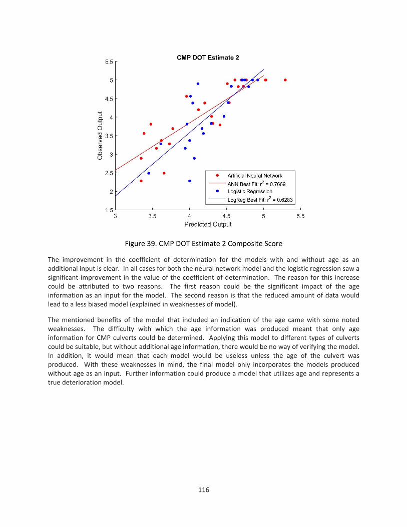
116

Figure 39. CMP DOT Estimate 2 Composite Score

The improvement in the coefficient of determination for the models with and without age as an additional input is clear. In all cases for both the neural network model and the logistic regression saw a significant improvement in the value of the coefficient of determination. The reason for this increase could be attributed to two reasons. The first reason could be the significant impact of the age information as an input for the model. The second reason is that the reduced amount of data would lead to a less biased model (explained in weaknesses of model).

The mentioned benefits of the model that included an indication of the age came with some noted weaknesses. The difficulty with which the age information was produced meant that only age information for CMP culverts could be determined. Applying this model to different types of culverts could be suitable, but without additional age information, there would be no way of verifying the model. In addition, it would mean that each model would be useless unless the age of the culvert was produced. With these weaknesses in mind, the final model only incorporates the models produced without age as an input. Further information could produce a model that utilizes age and represents a true deterioration model.

117

Appendix B: Copy of the Risk Assessment Survey

Figure 40. Barrel Failure Risk Assessment Survey

119

Appendix C: Failure Risk Analysis Results

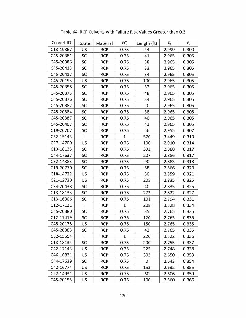
120

Table 64. RCP Culverts with Failure Risk Values Greater than 0.3

Culvert ID Route Material FCj Length (ft) Cj Rj

C13‐19367 US RCP 0.75 44 2.999 0.300

C45‐20381 SC RCP 0.75 41 2.965 0.305

C45‐20386 SC RCP 0.75 38 2.965 0.305

C45‐20413 SC RCP 0.75 33 2.965 0.305

C45‐20417 SC RCP 0.75 34 2.965 0.305

C45‐20193 US RCP 0.75 100 2.965 0.305

C45‐20358 SC RCP 0.75 52 2.965 0.305

C45‐20373 SC RCP 0.75 48 2.965 0.305

C45‐20376 SC RCP 0.75 34 2.965 0.305

C45‐20382 SC RCP 0.75 0 2.965 0.305

C45‐20384 SC RCP 0.75 38 2.965 0.305

C45‐20387 SC RCP 0.75 40 2.965 0.305

C45‐20407 SC RCP 0.75 43 2.965 0.305

C19‐20767 SC RCP 0.75 56 2.955 0.307

C32‐15143 I RCP 1 570 3.449 0.310

C27‐14700 US RCP 0.75 100 2.910 0.314

C13‐18135 SC RCP 0.75 392 2.888 0.317

C44‐17637 SC RCP 0.75 207 2.886 0.317

C32‐14383 SC RCP 0.75 90 2.883 0.318

C19‐20770 SC RCP 0.75 88 2.866 0.320

C18‐14722 US RCP 0.75 50 2.859 0.321

C21‐12730 US RCP 0.75 205 2.835 0.325

C34‐20438 SC RCP 0.75 40 2.835 0.325

C13‐18133 SC RCP 0.75 272 2.822 0.327

C13‐16906 SC RCP 0.75 101 2.794 0.331

C12‐17131 I RCP 1 208 3.328 0.334

C45‐20380 SC RCP 0.75 35 2.765 0.335

C12‐17419 SC RCP 0.75 120 2.765 0.335

C45‐20178 US RCP 0.75 150 2.765 0.335

C45‐20383 SC RCP 0.75 42 2.765 0.335

C32‐15554 I RCP 1 220 3.322 0.336

C13‐18134 SC RCP 0.75 200 2.755 0.337

C42‐17143 US RCP 0.75 225 2.748 0.338

C46‐16831 US RCP 0.75 302 2.650 0.353

C44‐17639 SC RCP 0.75 0 2.643 0.354

C42‐16774 US RCP 0.75 153 2.632 0.355

C22‐14931 US RCP 0.75 60 2.606 0.359

C45‐20155 US RCP 0.75 100 2.560 0.366

121

C12‐17421 SC RCP 0.75 24 2.484 0.377

C21‐12733 US RCP 0.75 138 2.367 0.395

C45‐20385 SC RCP 0.75 40 2.355 0.397

C42‐17082 US RCP 0.75 248 2.322 0.402

C34‐19375 US RCP 0.75 57 2.280 0.408

C20‐16815 I RCP 1 371 2.950 0.410

C27‐15207 I RCP 1 626 2.921 0.416

C21‐20234 SC RCP 0.75 60 2.195 0.421

C21‐20237 SC RCP 0.75 60 2.195 0.421

C12‐18084 SC RCP 0.75 44 2.141 0.429

C17‐20784 SC RCP 0.75 56 2.038 0.444

C17‐20792 SC RCP 0.75 50 2.029 0.446

C42‐17115 US RCP 0.75 350 2.025 0.446

C23‐17703 SC RCP 0.75 54 1.866 0.470

C44‐17035 US RCP 0.75 288 1.825 0.476

C45‐20164 SC RCP 0.75 41 1.625 0.506

C17‐20787 SC RCP 0.75 174 1.067 0.590

C45‐20486 US RCP 0.75 45 1.000 0.600

C45‐20375 SC RCP 0.75 48 0.800 0.630

C13‐19368 US RCP 0.75 40 0.600 0.660

C46‐18585 SC RCP 0.75 170 0.200 0.720

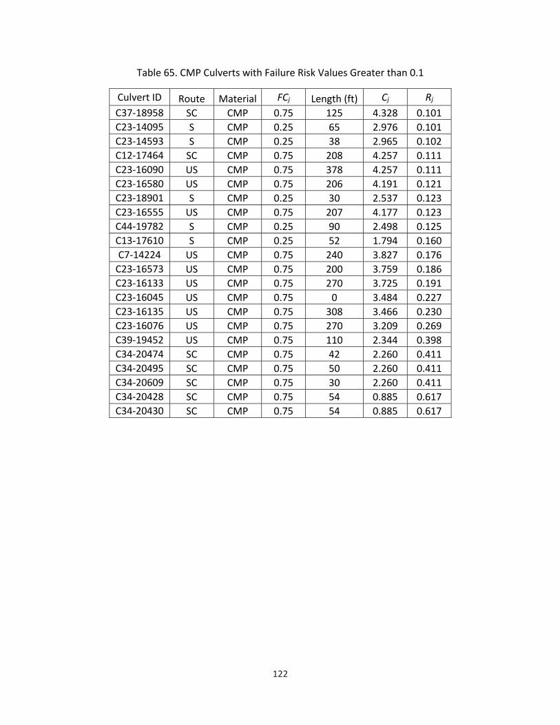
122

Table 65. CMP Culverts with Failure Risk Values Greater than 0.1

Culvert ID Route Material FCj Length (ft) Cj Rj

C37‐18958 SC CMP 0.75 125 4.328 0.101

C23‐14095 S CMP 0.25 65 2.976 0.101

C23‐14593 S CMP 0.25 38 2.965 0.102

C12‐17464 SC CMP 0.75 208 4.257 0.111

C23‐16090 US CMP 0.75 378 4.257 0.111

C23‐16580 US CMP 0.75 206 4.191 0.121

C23‐18901 S CMP 0.25 30 2.537 0.123

C23‐16555 US CMP 0.75 207 4.177 0.123

C44‐19782 S CMP 0.25 90 2.498 0.125

C13‐17610 S CMP 0.25 52 1.794 0.160

C7‐14224 US CMP 0.75 240 3.827 0.176

C23‐16573 US CMP 0.75 200 3.759 0.186

C23‐16133 US CMP 0.75 270 3.725 0.191

C23‐16045 US CMP 0.75 0 3.484 0.227

C23‐16135 US CMP 0.75 308 3.466 0.230

C23‐16076 US CMP 0.75 270 3.209 0.269

C39‐19452 US CMP 0.75 110 2.344 0.398

C34‐20474 SC CMP 0.75 42 2.260 0.411

C34‐20495 SC CMP 0.75 50 2.260 0.411

C34‐20609 SC CMP 0.75 30 2.260 0.411

C34‐20428 SC CMP 0.75 54 0.885 0.617

C34‐20430 SC CMP 0.75 54 0.885 0.617

123

Appendix D: Case Studies for Validation

124

Tables 66, 67 and 68 present the details of various real‐world case studies that were document for validating the CREST model.

Table 66. Practical Case studies for RCP Applications

Case Year Owner Contractor Location Shape Size (in)

Length (ft)

Major defect


References

1 Unknown UDOT Unknown Unknown Circular 24 18 Crack SL Contech, 2016

2 2014 Lakehurst Naval

Air Station Sequoia Construction

& Heitkamp Inc. Unknown Circular 48 786 ID SWL

Contech, 2014a

3 2014 Lakehurst Naval

Air Station Sequoia Construction

& Heitkamp Inc. Unknown Circular 54 703 ID SWL

Contech, 2014a

4 2012 WDOT Michels Corporation Mitchell

Interchange on I‐94, Wisconsin

Circular 54 300 Crack SL Contech, 2012a

5 2010 VAOT Morrill

Construction Interstates 89 and

91, Vermont Circular 96 500 ID SL

Contech, 2010

6 2012 Bradford County Florida

Engineered Lining Bradford County, Pennsylvania

Box 120 80 ID SL Contech, 2012b

7 2013 IDOT Brandt

Construction Co. I‐74 and I‐80 in Moline, Illinois

Circular 144 360*2 ID SL Contech, 2013

8 2012 NHDOT Weaver Brothers

Construction Co Inc. Route 123,

New Hampshire Circular 72 Unknown Multiple SL

Contech, 2012c

9 2014 MEDOT Prock Marine Company

U.S. Route 1, Maine

Circular 96 42 Multiple (ID, Crack)

SL Contech, 2014b

10 2014 Mobile Regional

Airport John G. Walton, Inc. Indiana Reline, Inc.

Mobile Regional Airport, Alabama

Circular 120 1500 Multiple (ID, Crack)

SL Contech, 2014c

125

Table 67. Practical case studies for CMP applications (1)


Length (ft)

Major defect


References

11 2010 Transportation of Quebec

Insituform Highway 640 in

Boisbriand, Québec Circular 36 160 Corrosion CIPP

Insituform, 2010




Insituform, 2010

13 2010 MnDOT District 6 Wabasha, MN

Unknown Unknown Circular 36 80 Corrosion CCCP MDOT, 2012

14 2013 UDOT Dennis Lierd Construction

State Route 201, Utah Circular 45 550 Corrosion SWL MDOT, 2012


Insituform Highway 640 in Boisbriand, Québec

Circular 48 260 Corrosion CIPP Insituform,

2010




Insituform, 2010

17 Unknown Keowee Key Golf

Course & Country Club

Milliken Keowee Key Golf Course and Country Club, SC

Circular 60 220 Corrosion CCCP Milliken, 2015a

18 2013 Henrico County

Virginia Milliken

Byrdhill Rd, Virginia

Circular 66 25 Corrosion CCCP Milliken, 2013

19 2015 Alabama & Gulf Coast Railway

Chase Plumbing & Mechanical, Inc.

Alabama & Gulf Coast Railway, Alabama

Circular 132 106 Corrosion SL Contech, 2015a

126

Table 68. Practical case studies for CMP applications (2)


Length (ft)

Major defect


References

20 2014 Sheboygan County

Sheboygan County Lakeshore Road and

Najacht Road, Wisconsin Circular 74 38*2 ID SL

Contech, 2014e

21 2014 Scott

Air Force Base

Davinroy Mechanical

Contractors Inc

St. Clair County, Illinois

Ellipse 72 2208 ID SL Contech, 2015b

22 Unknown community of

Walden on Lake Conroe

Milliken Walden on Lake Conroe,

Texas Circular 66 130

Multiple (Corrosion,

ID) CCCP

Milliken, 2015c

23 Unknown City of

Rock Springs Milliken Unknown Arch 72 700

Multiple (ID, JI)

CCCP Milliken, 2015d

24 2012 City of

Campbell River Upland Excavating

Ltd.

Coast of British Columbia, Canada

Circular 120 86 Multiple SL Contech, 2012d

25 2013 UDOT Dennis Lierd Construction

State Route 201, Utah

Circular 18~36 6000 Corrosion SL Contech, 2014d

26 Unknown McAllen Texas

Milliken Rio Grande,

Texas Circular 120 300 JI CCCP

Milliken, 2015b

127

7. REFERENCES

<http://oceanpipe.com/sites/oceanpipe.com/files/PDFs/installation‐information/AASHTO%20Post%20Installation%20Inspection%20Guideline.pdf> (May 4th, 2016).

AASHTO. (2009). “AASHTO Post Installation Inspection Guideline.”

Adamtey, S.A., Onsarigo, L., and Atalah, A. (2015). Case Study of the Replacement of Corrugated Metal Culverts Using Pipe Bursting. 2016 No‐Dig Conference, Dallas, Texas.

Adamtey, S.A., 2016. Replacement of corrugated metal pipe culverts using pipe bursting (Doctoral dissertation, INDIANA STATE UNIVERSITY).

Agarwal, M. (2010). “Developing a Framework for Selecting Condition Assessment Technologies for Water and Wastewater Pipes” Master Dissertation in Civil Engineering, Virginia Polytechnic Institute and State University.

Aimin, Y., Jintao, L., Bohai, J., and Haifeng, M. (2011) Study on Damage Identification for a Simply Supported Reinforced Concrete Beam Based on the LMBP Neural Network. Design, Construction, Rehabilitation, and Maintenance of Bridges: pp. 65‐72. doi: 10.1061/47630(409)9

Al‐Gburi, Majid A., Jan‐Erik Jonasson, and Martin Nilsson. "Using Artificial Neural Networks to Predict the Restraint in Concrete Culverts at Early Age." Structural Engineering International 25.3 (2015): 258‐65. Web.

American Concrete Pipe Association (ACPA). (2007). “HDPE Pipe Service Life.” Accessed at: http://www.concretepipe.org/wp‐content/uploads/2015/05/YSK‐142‐HDPE‐Pipe‐Service‐Life.pdf, on August 1st, 2016.

Ana, E. V., and W. Bauwens. "Modeling the Structural Deterioration of Urban Drainage Pipes: The State‐of‐the‐art in Statistical Methods." Urban Water Journal 7.1 (2010): 47‐59. Web.

Ariaratnam, Samuel T., Ashraf El‐Assaly, and Yuqing Yang. "Assessment of Infrastructure Inspection Needs Using Logistic Models." J. Infrastruct. Syst. Journal of Infrastructure Systems 7.4 (2001): 160‐65. Web.

Baik, Hyeon‐Shik, Hyung Seok Jeong, and Dulcy M. Abraham. "Estimating Transition Probabilities in Markov Chain‐Based Deterioration Models for Management of Wastewater Systems." J. Water Resour. Plann. Manage. Journal of Water Resources Planning and Management 132.1 (2006): 15‐24. Web.

128

Ballinger, C. A., and Drake, P. G. (1995). “Culvert Repair Practices Manual: Volume1.” RD‐94‐096, Federal Highway Administration, Mclean, VA.

Beaver, Jesse L., Timothy J. Mcgrath, and Blaine Leonard. "Condition Assessment of Utah Highway Culverts and Determination of Culvert Performance Measures." Critical Transitions in Water and Environmental Resources Management (2004): n. pag. Web.

California Department of Transportation (Caltrans). (2013) “Design Information Bulletin No. 83 ‐ 03Caltrans Supplement to FHWA Culvert Repair Practices Manual.” Accessed at: http://www.dot.ca.gov/hq/oppd/dib/dib83‐03.pdf, on May 1st, 2015.

Contech. (2010). “I‐89 Relines, Quimby Mountain Rd & Exit 2.” <http://www.conteches.com/KnowledgeCenter/CaseStudies/CaseStudyDetails?articleId=674>.

Contech. (2012a). “I‐94 Reline at Mitchell Interchange.”

< http://www.conteches.com/knowledge‐center/case‐studies/case‐study‐details/articleid/678/i‐94‐reline‐at‐mitchell‐interchange>.

Contech. (2012b). “Bradford County Reline.” <http://www.conteches.com/KnowledgeCenter/CaseStudies/CaseStudyDetails?articleId=443>.

Contech. (2012c). “NHDOT State Route 123.” <http://www.conteches.com/KnowledgeCenter/CaseStudies/CaseStudyDetails?articleId=828>.

Contech. (2012d). “Galerno Road over Simms Creek Reline.” <http://www.conteches.com/KnowledgeCenter/CaseStudies/CaseStudyDetails?articleId=978>.

Contech. (2013). “Henry County – IDOT I‐74/280 Reline.” <http://www.conteches.com/KnowledgeCenter/CaseStudies/CaseStudyDetails?articleId=1146>.

Contech. (2014a). “Lakehurst Naval Air Station – Reline.” <http://www.conteches.com/KnowledgeCenter/CaseStudies/CaseStudyDetails?articleId=1136>.

Contech. (2014b). “US Route 1 ‐ Warren, Maine Culvert Replacement.” <http://www.conteches.com/KnowledgeCenter/CaseStudies/CaseStudyDetails?articleId=1310>.

Contech. (2014c). “Mobile Regional Airport ‐ Runway 14/32.” <http://www.conteches.com/KnowledgeCenter/CaseStudies/CaseStudyDetails?articleId=1148>.

129

Contech. (2014d). “UDOT SR201 and I‐80 Reline.” <http://www.conteches.com/KnowledgeCenter/CaseStudies/CaseStudyDetails?articleId=1460> .

Contech. (2014e). “Lakeshore & Najacht Road Reline.” <http://www.conteches.com/KnowledgeCenter/CaseStudies/CaseStudyDetails?articleId=1496>.

Contech. (2015a). “Alabama & Gulf Coast Railway Reline.” <http://www.conteches.com/KnowledgeCenter/CaseStudies/CaseStudyDetails?articleId=1496>.

Contech. (2015b). “Scott Air Force Base Drainage Improvements.” <http://www.conteches.com/KnowledgeCenter/CaseStudies/CaseStudyDetails?articleId=1179>.

Contech. (2016). “Cornia Drive.” <http://www.conteches.com/KnowledgeCenter/CaseStudies/CaseStudyDetails?articleId=520>.

Contech Engineered Solutions. (2016). “Corrugated Metal Pipe” Accessed at: http://www.conteches.com/DesktopModules/Bring2mind/DMX/Download.aspx?command=core_download&entryid=1940&language=en‐US&PortalId=0&TabId=144, on August 1st, 2016.

Cook, R. Dennis; Weisberg, Sanford (1982). Residuals and Influence in Regression. (Repr. ed.). New York: Chapman and Hall. ISBN 041224280X. Retrieved 3 September 2016.

Costello, S. B., Chapman, D. N., Rogers, C. D. F., and Metje, N. (2007). “Underground asset location and condition assessment technologies.” Tunneling and Underground Space Technology, 22, 524–542.

Derr, K., and Hubbard, P. (2009). “In‐service Inspection of Wastewater Force Mains.” Pipelines 2009, 360, 249‐260.

Ennaouri, I., and Musandji Fuamba, M. (2013). “New Integrated Condition‐Assessment Model for Combined Storm‐Sewer Systems” Journal of Water Resources Planning and Management, 139(1), 53‐64.

Fawcett, Tom. "An Introduction to ROC Analysis." Pattern Recognition Letters27.8 (2006): 861‐74. Web.

FHWA. (2010). “Culvert Assessment and Decision Making Procedures Manual. Lakewood, CO.” <http://www.cflhd.gov/programs/techDevelopment/hydraulics/culvertassessment/01_Culvert_Assessment_Decision_Making_Proceudres_Manual.pdf> (May 1, 2015).

Hao, T., Rogers, C.D.F., Metje, N., Chapman, D. N., Muggleton, J. M.., Foo, K. Y., Wangd, P., Pennock, S. R.., Atkins, P. R.., Swingler, S. G., Parker, J., Costello, S. B., Burrow, M. P. N.,

130

Anspach, J. H., Armitage, R. J., Cohn, A. G., Goddard, K., Lewin, P. L., Orlando, G., Redfern, M. A., Royal, A. C. D., and Saul, A. J.. (2012). “Condition Assessment of the Buried Utility Service Infrastructure.” Tunneling and Underground Space Technology, 28, 331‐344

Hollingshead, T., and Tullis, B. P. (2009). “In‐Situ Culvert Rehabilitation: Synthesis Study and Field Evaluation.” Report No. UT‐09.16, Utah Department of Transportation, Salt Lake, Utah.

Hunt, J. H., Zerges, S. M., Roberts, B. C., and Bergendahl, B. (2010). “Culvert Assessment and Decision‐Making Procedures Manual for Federal Lands Highway.” Publication No. FHWA‐CFL/TD‐10‐005, Federal Highway Administration Central Federal Lands Highway Division, Lakewood, CO.

Insituform. (2010). “MTQ Rehabilitates Highway Culverts.” <http://www.insituform.com/AboutUs/CaseStudies/NACaseStudies/Canadian‐Culvert‐Rehab>.

International Pipe Bursting Association (IPBA) (2012). “Guideline for Pipe Bursting.” Available at: http://www.teamipr.com/pdf/specification‐pipebursting.pdf

J., Colorado Urrea Gabriel. Service Life of Concrete and Metal Culverts Located in Ohio Department of Transportation Districts 9 and 10. Thesis. Ohio University, December, 2014. N.p.: n.p., n.d. Print.

Karamouz, M., Yousefi, M., Zahmatkesh, Z., and Nazif, S. (2012). “Development of an Algorithm for Vulnerability Zoning of Water Distribution Network.” Proceedings of the World Environmental and Water Resources Congress 2012: Crossing Boundaries, 3011‐3020.

Kleiner, Yehuda, and Balvant Rajani. "Comprehensive Review of Structural Deterioration of Water Mains: Statistical Models." Urban Water 3.3 (2001): 131‐50. Web.

Kleiner, Yehuda, Balvant Rajani, and Rehan Sadiq. "Failure Risk Management of Buried Infrastructure Using Fuzzy‐based Techniques." J Water Supply Res Tec Journal of Water Supply: Research and Technology ‐ Aqua 55.2 (2006): 81‐94. Web.

Lanzo Lining Services, Inc. (LLSI). (2010). “Engineering Design Guide for Rehabilitation with Cured‐In‐Place Pipe.” Accessed at: http://lanzo.net/pdf/lanzo‐lining‐guide‐2410.pdf, on May 1st, 2015.

Liriano, S. L., & Day, R. (2001). Prediction of scour depth at culvert outlets using neural networks. Journal of Hydroinformatics, 3(4), 231‐238.

Liu, Z., Kleiner, Y., and Rajani, B. (2012). “Condition Assessment Technologies for Water Transmission and Distribution Systems.” Institute for Research in Construction National Research Council Canada Ottawa, Ontario, Canada.

131

Marquardt, Donald W. "An Algorithm for Least‐Squares Estimation of Nonlinear Parameters." Journal of the Society for Industrial and Applied Mathematics 11.2 (1963): 431‐41. Web.

MATLAB, Statistics Toolbox, and Neural Network Toolbox Release 2015a, The MathWorks, Inc., Natick, Massachusetts, United States.

Matthews, J. C., Simicevic, J., Kestler, M. A., and Piehl, R. (2012). “Decision Analysis Guide for Corrugated Metal Culvert Rehabilitation and Replacement Using Trenchless Technology.” 1177 1810‐STDDC, United States Department of Agriculture, Washington, D.C.

Meegoda, J. N., Juliano, T. M., and Tang, C., (2009). “Culvert Information Management System – Demonstration Project.” FHWA‐NJ‐2009‐017, New Jersey Department of Transportation, Trenton, NJ.

Meegoda, Jay N. and Thomas M. Juliano. Corrugated Steel Culvert Pipe Deterioration. New Jersey Department of Transportation Bureau of Research and Federal Highway Administration, 2009. Print.

Meegoda, Jay N., and Zhenting Zou. "Long‐Term Maintenance of Culvert Networks." J. Pipeline Syst. Eng. Pract. Journal of Pipeline Systems Engineering and Practice 6.4 (2015): 04015003. Web.

Meegoda, Jay N., Thomas M. Juliano, Mutiu G. Ayoola, and Sunil Dhar, "A Methodology to Predict the Remaining Service Life of Cscps" (April 13, 2004). International Conference on Case Histories in Geotechnical Engineering. Paper 8.

Micevski, Tom, George Kuczera, and Peter Coombes. "Markov Model for Storm Water Pipe Deterioration." J. Infrastruct. Syst. Journal of Infrastructure Systems8.2 (2002): 49‐56. Web.

Milliken. (2013). “Geospray® Geopolymer: Culvert Relining.” <http://infrastructure.milliken.com/pages/case‐studies/detail/0/22/>.

Milliken. (2015a). “Geospray® Geopolymer: Culvert Rehabilitation.” <http://infrastructure.milliken.com/pages/case‐studies/detail/0/23/>.

Milliken. (2015b). “Geospray® Geopolymer: Storm Water Rehab.” <http://infrastructure.milliken.com/geospray‐storm‐water‐rehab‐case‐study/>.

Milliken. (2015c). “Geospray® Geopolymer: Corrugated Metal Storm Sewer.”

<http://infrastructure.milliken.com/pages/case‐studies/detail/0/20/>.

Milliken. (2015d). “Geospray® Geopolymer: Arched Storm Culvert.” <http://infrastructure.milliken.com/geospray‐arched‐storm‐culvert‐case‐study/>.

132

Minesota Department of Transportation (MDOT). (2012). “Culvert Repair Best Practices, Specifications, and Special Provisions: Task C Research Synthesis.” Minesota Department of Transportation, Minesota.

Mitchell, G. F., Masada, T., Sargand, S. M., and Jobes Henderson & Associates, Inc. (2005). “Risk Assessment and Update of Inspection Procedures for Culverts.” FHWA/OH‐2005/002, Ohio Department of Transportation, Columbus, OH.

Monographs on Statistic and Applied Probability. London: Chapman & Hall., n.d. Print.

Najafi, M., and Bhattachar, D. V. (2011). “Development of a Culvert Inventory and Inspection Framework for Asset Management of Road Structures.” J. King Saud University Science, 23(3), 243–254.

Najafi, M., Salem, S., Bhattachar, D., Salman, B., Patil, R.., and Calderon, D. (2008). “An Asset Management Approach for Drainage Infrastructures & Culverts.” Midwest Regional University Transportation Center, University of Wisconsin‐Madison, Madison, WI 53706.

Najafi, Mohammad, and Guru Kulandaivel. "Pipeline Condition Prediction Using Neural Network Models." Pipelines 2005 (2005): n. pag. Web.

National Cooperative Highway Research Program (NCHRP). (2002). “Assessment and Rehabilitation of Existing Culverts.” Transportation Research Board – the National Academies, Washington, D.C.

Ohio Department of Transportation (ODOT). (2003). "Culvert management manual." <https://www.dot.state.oh.us/Divisions/Engineering/Hydraulics/Culvert%20Management/Culvert%20Management%20Manual/CMM%20‐%20July%202015.pdf> (May 1st, 2015).

PCA. (2015). “Shotcrete.” <http://www.cement.org/concrete‐basics/concrete‐homes/building‐systems‐for‐every‐need/shotcrete>.

Perrin, Jr., and Jhaveri, C. S. (2004). “The Economic Costs of Culvert Failures.” Proceedings of the 83rd Annual Meeting of the Transportation Research Board, Washington, D.C.

ProjectMax. (2006). “Rehabilitation of Sewer Pipelines.” Accessed at: http://www.projectmax.co.nz/_literature_43894/overview_of_sewer_rehabilitation, on May 1st, 2015.

Rumpca, A. H. (1998). “Evaluation of High Density Polyethylene (HDPE) Pipe.” SD96‐11‐F, South Dakota Department of Transportation, Pierre, SD.

Saaty, L. S. (2008). “Decision Making with the Analytic Hierarchy Process.” Int. J. Services Sciences, 1, 83‐98.

Saaty, R. W. (1987). The analytic hierarchy process—what it is and how it is used. Mathematical Modelling, 9(3), 161‐176.

133

Salem, Ossama, Baris Salman, and Mohammad Najafi. "Culvert Asset Management Practices and Deterioration Modeling." Transportation Research Record: Journal of the Transportation Research Board 2285 (2012): 1‐7. Web.

SCDOT, “Pipe & Culvert Inventory and Assessment Guidelines,” 2011.

Selvakumar, A., Tuccillo, M. E., Martel, K. D., Matthews, J. C., and Feeney, C. (2014). “Demonstration and Evaluation of State‐of‐the‐Art Wastewater Collection Systems Condition Assessment Technologies.” Journal of Pipeline Systems Engineering and Practice, 5(2), 1949‐1190.

Sheela, K. Gnana, and S. N. Deepa. "Review on Methods to Fix Number of Hidden Neurons in Neural Networks." Mathematical Problems in Engineering 2013 (2013): 1‐11. Web.

South Carolina Department of Transportation, “Requirements for Hydraulic Design Studies,” SCDOT, 2009. www.scdot.org

Stocking, A. (2013). “Three Trenchless Culvert‐Rehab Solutions.” Accessed at: http://www.pwmag.com/pipes/three‐trenchless‐culvert‐rehab‐solutions.aspx,on May 1st, 2015.

Syachrani, S., Jeong, H. S., Rai, V., Chae, M., and Iseley, T. (2010). “A Risk Management Approach to Safety Assessment of Trenchless Technologies for Culvert Rehabilitation.” Tunnelling and Underground Space Technology, 25, 681–688.

Tatari, Omer, Shad M. Sargand, Teruhisa Masada, and Bashar Tarawneh. "Neural Network Approach to Condition Assessment of Highway Culverts: Case Study in Ohio." J. Infrastruct. Syst. Journal of Infrastructure Systems 19.4 (2013): 409‐14. Web.

The Welding Institute (TWI). (2016). “What are the Advantages and Disadvantages of Ultrasonic Examination in Non‐Destructive Examination?” <http://www.twi‐global.com/technical‐knowledge/faqs/ndt/faq‐what‐are‐the‐advantages‐and‐disadvantages‐of‐ultrasonic‐examination‐in‐non‐destructive‐examination‐nde/> (June 18th, 2016).

Thompson, Paul D., Kevin M. Ford, and Mohammad H. R. Arman. Estimating Life Expectancies of Highway Assets. Washington, D.C. Transportation Research Board, 2012. Print.

Thornton C. I., Robeson, M. D., Girard, L. G., and Smith, B. A. (2005). “Culvert Pipe Liner Guide and Specifications.” FHWA‐CFL/TD‐05‐003, Federal Highway Administration Central Federal Lands Highway Division, Lakewood, CO.

Tran, D. H., A. W. M. Ng, B. J. C. Perera, S. Burn, and P. Davis. "Application of Probabilistic Neural Networks in Modelling Structural Deterioration of Stormwater Pipes." Urban Water Journal 3.3 (2006): 175‐84. Web.

Tran, H. D., B. J. C. Perera, and A. W. M. Ng. "Predicting Structural Deterioration Condition of Individual Storm‐Water Pipes Using Probabilistic Neural Networks and Multiple Logistic

134

Regression Models." J. Water Resour. Plann. Manage. Journal of Water Resources Planning and Management 135.6 (2009): 553‐57. Web.

Tran, Huu Dung. Investigation of Deterioration Models for Stormwater Pipe Systems. Thesis. 2007. N.p.: n.p., n.d. Print.

Trenchless Technology Magazine. (2006). “Trenchless Technology from Owner’s Perspective.” Accessed at: http://trenchlessonline.com/trenchless‐technology‐from‐the‐owners‐perspective, on May 1st, 2015.

Trenchless Technology Magazine. (2014). “2014 Pipe Relining Guide.” Accessed at: http://www.trenchlessonline.com/pdfs/2014‐pipe‐relining‐guide.pdf, on August 1st, 2016.

Tuccillo, M. E., Jolley, J., Martel, K., and Boyd, G. (2010). “Report on Condition Assessment Technology of Wastewater Collection Systems.” U.S. Environmental Protection Agency (USEPA), Ohio.

U.S. Environmental Protection Agency (US EPA). (2015). “Water Technology Fact Sheet.” Accessed at: http://water.epa.gov/scitech/wastetech/upload/2006_10_16_mtb_pipebursting_final.pdf, on May 1st, 2015.

Verma, Snajeev Kumar, Sudhir Singh Bhadauria, and Saleem Akhtar. “Estimating Residual Service Life of Deteriorated Reinforced Concrete Structures.” American Journal of Civil Engineering and Architecture AJCEA 1.5 (2013): 92‐96. Web.

Wyant, David C. Assessment and Rehabilitation of Existing Culverts. Washington, D.C. Transportation Research Board, 2002. Print.

Yang, C and Allouche, E. (2009). "Evaluation of Non‐destructive Methods for Condition Assessment of Culverts and Their Embedment." ICPTT 2009, 361, 28‐38

Yang, C. (2011). “Predicting Deterioration Rate of Culvert Structures Utilizing a Markov Model.” Doctoral Dissertation, College of Engineering and Science, Louisiana Tech University, Ruston, LA.

Yang, C. (2011). “Predicting Deterioration Rate of Culvert Structures Utilizing a Markov Model.” Doctoral Dissertation, College Of Engineering and Science Louisiana Tech University, Ruston, LA.

Yang, C. and Allouche, E. (2009). "Evaluation of Non‐destructive Methods for Condition Assessment of Culverts and Their Embedment." ICPTT 2009,361, 28‐38.

Yang, Chenguang, and Erez Allouche. "Evaluation of Non‐Destructive Methods for Condition Assessment of Culverts and Their Embedment." Icptt 2009 (2009): n. pag. Web.

135

Yazdekhasti, S., Piratla, K. R., Khan, A. and Atamturktur, S. (2014). “Analysis of Factors Influencing the Selection of Water Main Rehabilitation Methods,” NASTT No Dig 2014, Orlando, FL.

Yoo, D., Kang, D, Jun, H, and Kim, J. (2014). “Rehabilitation Priority Determination of Water Pipes Based on Hydraulic Importance.” Water, 6(12), 3864‐3887.

Best Practices for Assessing Health and Determining ... · i Final Report Best Practices for...

Documents

Transcript of Best Practices for Assessing Health and Determining ... · i Final Report Best Practices for...