Best Fit and Selection of Probability Distribution Models for Frequency Analysis of Extreme Mean...
20
International Journal of Engineering Research and Development e-ISSN: 2278-067X, p-ISSN: 2278-800X, www.ijerd.com Volume 11, Issue 04 (April 2015), PP.34-53 34 Best Fit and Selection of Probability Distribution Models for Frequency Analysis of Extreme Mean Annual Rainfall Events EM Masereka 1 , FAO Otieno 2 , GM Ochieng 3 J Snyman 4 1 D.Tech. student Civil Engineering Department, Tshwane University of Technology, Pretoria, South Africa 2 Prof and Vice Chancellor, Durban University of Technology, Durban, South Africa 3 Prof and Head of Dept; Civil Engineering and Building, Vaal University of Technology, Vanderbijlpark, South Africa 4 Dr, J. Snyman; Senior Lecturer Dept; Civil Engineering and Building Tshwane University of Technology; Pretoria South Africa Abstract:- Frequency analysis of extreme low mean annual rainfall events is important to water resource planners at catchment level because mean annual rainfall is an important parameter in determining mean annual runoff. Mean annual runoff is an important input in determining surface water available for water resource infrastructure development. In order to carry out frequency analysis of extreme low mean annual rainfall events, it is necessary to identify the best fit probability distribution models (PDMs) for the frequency analysis. The primary objective of the study was to develop two model identification criteria. The first criterion was developed to identify candidate probability distribution models from which the best fit probability distribution models were identified. The second criterion was applied to select the best fit probability distribution models from the candidate models. The secondary objectives were: to apply the developed criteria to identify the candidate and best fit probability distribution models and carry out frequency analysis of extreme low mean annual rainfall events in the Sabie river catchment which is one of water deficit catchments in South Africa. Although not directly correlated, mean annual rainfall determines mean annual runoff at catchment level. Therefore frequency analysis of mean annual rainfall events is important part of estimating mean annual runoff events at catchment level. From estimated annual runoff figures water resource available at catchment level can be estimated. This makes mean annual rainfall modeling important for water resource planning and management at catchment level. The two model identification criteria which were developed are: Candidate Model Identification Criterion (CMIC) and Least Sum of Statistics Model Identification Criterion (LSSMIC). CMIC and LSSMIC were applied to identify candidate models and best fit models for frequency analysis of distribution of extreme low mean annual rainfall events of the 8 rainfall zones in the Sabie river catchment. The mean annual rainfall data for the period 1920-2004 obtained from the Water Research Commission of South Africa was used in this study. Points below threshold method (PBTM) was applied to obtain the samples of extreme low mean annual rainfall events from each of the 8 rainfall zones. The long term mean of 85 years of each of the 8 rainfall zones was chosen as the threshold. The identification of the best-fit models for frequency analysis of extreme low mean annual rainfall events in each of the 8 rainfall zones was carried out in 2 stages. Stage 1 was the application of CMIC to identify candidate models. Stage 2 was the application of LSSMIC to identify the best fit models from the candidate models. The performance of CMIC and LSSMIC was assessed by application of Probability-Probability (P-P) plots. Although P-P plot results cannot be considered completely conclusive, CMIC and LSSMIC criteria make useful tools as model selection method for frequency analysis of extreme mean annual rainfall events. The results from the application of CMIC and LSSMIC showed that the best fit models for frequency analysis of extreme low mean annual rainfall events in the Sabie river catchment are; Log Pearson 3, Generalised Logistic and Extreme Generalised Value. Keywords:- Best-fit probability distribution function, Candidate probability distribution functions, candidate model identification criterion (CMIC) Least sum of statistics model selection criterion (LSSMIC) I. INTRODUCTION A. Water resources situation in South Africa South Africa is made of 19 water management areas (WMA), 11 of these water management areas are water deficit catchment where water resource demand is greater than the available water resource. Estimates carried out by Department of Water and Forestry indicate that by 2025 two or more additional Water
-
Upload
ijerd-editor -
Category
Technology
-
view
71 -
download
1
Transcript of Best Fit and Selection of Probability Distribution Models for Frequency Analysis of Extreme Mean...
International Journal of Engineering Research and Development
e-ISSN 2278-067X p-ISSN 2278-800X wwwijerdcom
Volume 11 Issue 04 (April 2015) PP34-53
34
Best Fit and Selection of Probability Distribution Models for
Frequency Analysis of Extreme Mean Annual Rainfall Events
EM Masereka1 FAO Otieno
2 GM Ochieng
3 J Snyman
4
1DTech student Civil Engineering Department Tshwane University of Technology
Pretoria South Africa 2Prof and Vice Chancellor Durban University of Technology Durban South Africa
3Prof and Head of Dept Civil Engineering and Building Vaal University of Technology
Vanderbijlpark South Africa 4Dr J Snyman Senior Lecturer Dept Civil Engineering and Building Tshwane
University of Technology Pretoria South Africa
Abstract- Frequency analysis of extreme low mean annual rainfall events is important to water resource
planners at catchment level because mean annual rainfall is an important parameter in determining mean annual
runoff Mean annual runoff is an important input in determining surface water available for water resource
infrastructure development In order to carry out frequency analysis of extreme low mean annual rainfall events
it is necessary to identify the best fit probability distribution models (PDMs) for the frequency analysis The
primary objective of the study was to develop two model identification criteria The first criterion was
developed to identify candidate probability distribution models from which the best fit probability distribution
models were identified The second criterion was applied to select the best fit probability distribution models
from the candidate models The secondary objectives were to apply the developed criteria to identify the
candidate and best fit probability distribution models and carry out frequency analysis of extreme low mean
annual rainfall events in the Sabie river catchment which is one of water deficit catchments in South Africa
Although not directly correlated mean annual rainfall determines mean annual runoff at catchment level
Therefore frequency analysis of mean annual rainfall events is important part of estimating mean annual runoff
events at catchment level From estimated annual runoff figures water resource available at catchment level can
be estimated This makes mean annual rainfall modeling important for water resource planning and management
at catchment level
The two model identification criteria which were developed are Candidate Model Identification Criterion
(CMIC) and Least Sum of Statistics Model Identification Criterion (LSSMIC)
CMIC and LSSMIC were applied to identify candidate models and best fit models for frequency analysis of
distribution of extreme low mean annual rainfall events of the 8 rainfall zones in the Sabie river catchment The
mean annual rainfall data for the period 1920-2004 obtained from the Water Research Commission of South
Africa was used in this study Points below threshold method (PBTM) was applied to obtain the samples of
extreme low mean annual rainfall events from each of the 8 rainfall zones The long term mean of 85 years of
each of the 8 rainfall zones was chosen as the threshold
The identification of the best-fit models for frequency analysis of extreme low mean annual rainfall events in
each of the 8 rainfall zones was carried out in 2 stages Stage 1 was the application of CMIC to identify
candidate models Stage 2 was the application of LSSMIC to identify the best fit models from the candidate
models The performance of CMIC and LSSMIC was assessed by application of Probability-Probability (P-P)
plots
Although P-P plot results cannot be considered completely conclusive CMIC and LSSMIC criteria make useful
tools as model selection method for frequency analysis of extreme mean annual rainfall events
The results from the application of CMIC and LSSMIC showed that the best fit models for frequency analysis of
extreme low mean annual rainfall events in the Sabie river catchment are Log Pearson 3 Generalised Logistic
and Extreme Generalised Value
Keywords- Best-fit probability distribution function Candidate probability distribution functions candidate
model identification criterion (CMIC) Least sum of statistics model selection criterion (LSSMIC)
I INTRODUCTION A Water resources situation in South Africa
South Africa is made of 19 water management areas (WMA) 11 of these water management areas are
water deficit catchment where water resource demand is greater than the available water resource Estimates
carried out by Department of Water and Forestry indicate that by 2025 two or more additional Water
Best Fit and Selection of Probability Distribution Models for Frequency Analysis of Extreme Mean Annualhellip
35
Management Areas will experience water deficit situation (IWMI 1998) Although only 11 out of 19 water
management areas are in situation of water resource deficit on average the whole country can be classified as
water stressed (IWMI 1998) The annual fresh water availability is estimated to be less than 1700msup3 per capita
The 1700msup3 per capita is taken as the threshold or index for water stress Prolonged periods of low rainfall
periods result into low production agricultural products
South Africa depends on surface water resources for most of its domestic industrial and irrigation
requirements (NWRS 2003) There are no big rivers in South Africa so the surface water resources are mainly
in form of runoff The estimated mean annual runoff under natural condition is 49000 M msup3a and the mean
annual rainfall is 465 mm (NWRS 2003) The utilizable groundwater exploitation potential is estimated at
7500Mm3a (NWRS 2003) Although not directly correlated the amount of mean annual runoff depends on the
amount of mean annual rainfall Mean annual run off and mean annual rainfall are important variables for water
resource planning at catchment level In planning water resource systems at catchment level it is necessary to
consider the impacts of extreme scenarios of both mean annual rainfall and mean annual runoff
B Modeling the distribution of extreme mean annual rainfall events
Modeling of the distribution of extreme mean annual rainfall events is based on the assumption that
these events are independent and identically distributed random events This process is called stochastic
modeling Stochastic modeling therefore involves developing mathematical models that are applied to
extrapolate and generate events based on sample data of those specific events Numerous Stochastic models
have been developed to extrapolate different aspects of hydro-meteorological events including mean annual run-
off mean annual rainfall temperature stream flow groundwater soil moisture and wind Shamir et al (2007)
developed stochastic techniques to generate input data for modeling small to medium catchments Furrer and
Katz (2008) studied generation of extreme stochastic rainfall events The general practice in stochastic analysis
of hydro-meteorological events including extreme mean annual rainfall has been to assume a probability
distribution function that is then applied in the analysis The focus of this study was to develop model
identification criteria for selecting the best fit probability distribution functions for frequency analysis of
extreme annual rainfall events and apply the developed criteria to identify the best fit models The identified
best fit models were applied in modeling the distribution of extreme mean annual rainfall events in Sabie river
catchment which is one of water deficit catchments in South Africa
C Methods of identifying best fit probability distribution functions for extreme mean annual rainfall events
In developing magnitude ndash return period models for frequency analysis of extreme mean annual rainfall
events like other extreme hydro meteorological events it is necessary to identify probability distribution
functions that best fit the extreme event data The methods for identifying best fit probability distribution
functions that have been applied include maximum likelihood method (Merz and Bloschl 2005 Willems et al
2007) L-moments based method (Hosking et al 1985 Hosking 1990) Akaike information criteria
(Akaike1973) and Bayesian information criteria(Schwarz1978) The reliability of identifying the best fit
models for hydro-meteorological frequency analysis has had some criticisms Schulze (1989) points out that
because of general short data non homogeneity and non stationary of sample data extrapolation beyond the
record length of the sample data may give unreliable results
Boven (2000) has outlined the below listed limitations of applying probability distribution functions in modeling
extreme of hydro-meteorological events eg floods-
The best fit probability distribution function of the parent events is unknown And different probability
distribution functions may give acceptable fits to the available data Yet extrapolation based on these
probability distribution functions may result in significantly different estimates of the design events
The fitted probability distribution function does not explicitly take into account any changes in the
runoff generation processes for higher magnitude event
Apart from the above criticisms a gap still remains in that a specific criteria to identify best-fit PDFs for extreme
hydro-meteorological events that is universally accepted in South Africa has not been developed ( Smither and
Schulze 2003)
This gap is addressed in this study by developing two model identification criteria based on data from Sabie
river catchment Sabie river catchment is water deficit catchment
D Probability Distribution functions for frequency analysis of extreme hydro- meteorological events in South
Africa
Log-Pearson 3 (LP3) probability distribution function has been recommended for design hydro-
meteorological events mostly flood and drought in South Africa (Alexander 1990 2001) Gorgens (2007) used
both the LP3 and General Extreme Value distribution and found the two models suitable for frequency analysis
Best Fit and Selection of Probability Distribution Models for Frequency Analysis of Extreme Mean Annualhellip
36
of extreme hydro meteorological events in South Africa However Mkhandi et al (2000) found that the Pearson
Type 3 probability distribution function fitted with parameter by method of PWM to be the most appropriate
distribution to use in 12 of the 15 relatively homogenous regions identified in South Africa (Smithers-JC
2002) Cullis et al (2007) and Gericke (2010) have specifically recommended for further research in developing
the methodologies of determining best fit PDFs for frequency analysis of extreme hydro-meteorological events
in South Africa (Smithers JC 2002) In this study two model identification criteria were developed to address
the problem of identifying best fit probability distribution functions for frequency analysis of extreme hydro
meteorological events specifically extreme mean annual rainfall events in water deficit catchments in South
Africa
E Uncertainty associated with modeling of extreme mean annual rainfall events
There is inherent uncertainty in modeling extreme mean annual rainfall like other extreme hydro-
meteorological events Yen et al (1986) identified 5 classes of uncertainties The classes are-
Natural uncertainty due to inherent randomness of natural process
Model uncertainty due to inability of the identified model to present accurately the systemrsquos true
physical behavior
Parameter uncertainty resulting from inability to quantify accurately the model inputs and parameters
Data uncertainty including measurement errors and instrument malfunctioning
Operational uncertainty that includes human factors that are not accounted for in modeling or design
procedure
Yue-Ping (2010) quotes Van Asselt (2000) to have classified uncertainty based on the modelerrsquos and decision
makersrsquo views In this case the two classes are model outcome uncertainty and decision uncertainty The aim of
statistical modeling of extreme hydro-meteorological events is to reduce the degree of uncertainty and the risks
associated to acceptable levels
F Limitations inherent in presently applied model selection criteria
The common practice in frequency analysis of extreme hydro meteorological events like extreme mean
annual rainfall has been that the modeler chooses a model for frequency analysis or chooses a set of models
from which he identifies the best-fit model to be applied for the frequency analysis (Laio et al 2009) The
following limitations have been identified in this approach which include among others the following
Subjectivity - This limitation arises from the fact that there is no consistent universally accepted
method of choosing a model to be applied or a set of candidate models from which the best fit can be
identified for frequency analysis In other words the choice depends on the experience of the modeler
and therefore subjective
Ambiguity - The limitation arises from the fact that two or more models may pass the goodness-of-fit
test Which one to choose for analysis then leads to ambiguity (Burnham and Anderson 2002) and
Parsimony - The case of parsimony is when the identified model mimics the sample data applied as
frequency analysis rather than the trend of the variable under consideration
Jiang (2014) has further outlined limitations of presently applied model selection criteria as
Effective sample size This arises from the fact that the size of the sample n may not be equal to data
points because of correlation
The dimension of the model This limitation is due to the fact that the number of parameters can affect
the model fitting process
The finite-sample performance and effectiveness of the penalty These limitations are due to the fact
that the penalty chosen may be subjective and
The criterion of Optimality This limitation is due to the fact that in the present criteria practical
considerations for instance economic or social factors are hardly included
The limitation of parameter under and over fitting to models has also been cited in the current model
selection criteria An attempt was made to address the above outlined limitations in developing the two model
selection criteria
II METHODS Developing two model identification criteria and applying the developed criteria for frequency analysis
of extreme low mean annual rainfall events in 8 rainfall zones in Sabie secondary catchment was carried out in 4
stages
1 Developing CMIC for identifying candidate model
Best Fit and Selection of Probability Distribution Models for Frequency Analysis of Extreme Mean Annualhellip
37
2 Developing LSSMSC for identifying the best fit models from the candidate models
3 Developing frequency analysis models based on the identified best fit models
4 Developing QT-T models for each extreme low mean rainfall event sample
A Development process of CMIC
The development of CMIC was made in two steps Step 1 was based on classification of PDFs and
bound characteristics of upper and lower tail events of the distributions of the sample data of the extreme low
mean annual rainfall The step 2 was based on set significance levels in hypothesis testing as explained below
1) Bounds classification and tail events characteristics of PDFs The step 1 of development of CMIC criterion
was based on the classification of continuous probability distribution functions and bound characteristics of
upper and lower tail events of the distributions of sample data Continuous probability distribution functions can
be divided into four classes Bounded Unbounded Non-Negative and Advanced (MathWave 2011) This
division is based on their upper and lower tail events characteristics and their functionality The lower and the
upper tail events of the samples were applied to develop CMIC because the extreme characteristics of a sample
are expressed in the spread of tail events Probability distribution function of events in any sample of any
variable has two bounds upper and lower tail events MathWave (2011) has proposed three possible
characteristics of any tail events bound These are - unknown open and closed These characteristics were
adopted
The rationale behind the three characteristics can be illustrated as follows Let sample M of variable X
be made of events X1 X2helliphelliphellipXn-1 Xn arranged in ascending order and the sample size is n If the sample
events X1 and Xn are defined and known then the sample comes from a parent population of frequency
distribution functions with both lower and upper tails bounded and the tails are closed These distributions are
called bounded with closed tails (MathWave 2011) If X1 and Xn events of M are undefined with unknown
value then the sample belongs to a parent population of frequency distribution which is unbounded with
unknown or open tails If X1 and Xn of the sample are positive then the sample belongs to a population of
frequency distribution with end tails which can be non-negative unknown open or closed The sample data that
does not belong to any of the above groups belongs to populations with advanced distribution functions
(MathWave 2011) Summary of distribution bounds is given in Table I
Table I Bound Classifications and Tail Characteristics of Distribution Functions
Upper
Lower
Unknown Open Closed
Unknown Bounded
Unbounded
Non-Negative
advanced
Unbounded
Non-Negative
Advanced
Bounded
Advanced
Open Unbounded
Advanced
Unbounded
Advanced
Advanced
Closed Bounded
Non-Negative
Advanced
Non-Negative
Advanced
Bounded
Advanced
Source (MathWave 2011)
The CMIC criterion for identifying sample specific candidate models for frequency analysis was based on Table
1 The development of CMIC involved the following basics
Let the sample M of variable X be made of events
21
If events are arranged in ascending order then
22
and if is the smallest numerical value event and forms the last event of lower tail of frequency distribution of
and is the largest numerical value event and forms the last event of upper tail of frequency distribution
of then in this case both upper and lower tails of are bounded defined and closed therefore the
candidate models for frequency analysis of are bounded and advanced with closed tails (Table1) There are
two extreme scenarios in this method Scenario one arises when numerical values X1 and Xn of a specific sample
events are unknown and undefined In this case all available continuous probability distribution functions are
Best Fit and Selection of Probability Distribution Models for Frequency Analysis of Extreme Mean Annualhellip
38
candidate models These models are bounded unbounded non- negative and advanced (Table I) The other
scenario is when the numerical values of X1 and X n are identified and defined numerical values In this case
bounded and advanced continuous probability distribution functions are the candidate models The step 1
procedure led to identification of the initial candidate models for frequency analysis of low and high extreme
mean rainfall sample data events
2) Hypothesis testing and significance levels This was step 2 of development of CMIC For initial candidate
models identified in Step 1 for each sample data hypothesis testing at significance levels 02 01 005 002 and
001was carried out
The goodness of fit tests adopted for this study were Kolomogrov-Smirnov Anderson-Darling and
Chi-Square The reasons for applying the 3 specific goodness of fit tests are outlined in section C
The null and the alternative hypothesis for each test were -
HO The sample data was best described by the specific probability distribution function
HA The sample data was not best described by the specific probability distribution function
The hypothesis testing was applied to fence-off the final candidate models from the initial candidate
models identified by bounds method Models from initial candidate models that were rejected in hypothesis
testing at any significance levels of 02 01 005 002 and 001 by any of the three goodness-of-fit tests were
dropped from the candidate models
B Development of Least Sum of the Statistic Model Identification Criterion (LSSMIC)
1) Introduction The Least Sum of the Statistic Model Selection Criterion (LSSMSC) was developed by
determining the Least Sum of Statistics of goodness of fit of the tests - Kolmogorov-Smirnov Anderson-
Darling and Chi-Square The mathematical principle of each of the tests on which development of LSSMSC
was based is briefly discussed below
2) Kolmogorov-Smirnov statistic Kolmogorov-Smirnov statistic is based on uniform law of large
numbers which is expressed in Glivenko-Cantelli Theorem (Wellener 1977)
The theorem can be summarized as
23
In this case is the cumulative distribution function is the empirical cumulative distribution function
defined by
24
where are iid with distribution and
The uniformity of this law for large numbers can be explained as
25
26
where is the empirical distribution that assigns to each
The law of large numbers indicates that for all
According to GLivenkondashCantelli theorem (Wellner 1977) this happens uniformly over Applications of
Kolmogorov-Smirnov statistic as an index in determining the best-fit model among the candidate models was
based on this theorem The model with the Least Kolmogorov-Smirnov statistic was taken as the best fit model
for this test since as in equation 26
3) Anderson-Darling statistic Anderson-Darling statistic is an index of goodness-ofndashfit test In this
case the Anderson-Darling goodness-ofndashfit test is the comparison of empirical distribution function
assumed to be the parent distribution that is the distribution being fitted to sample data
The hypothesis is
Ho 27
The hypothesis is rejected if is very different from
Best Fit and Selection of Probability Distribution Models for Frequency Analysis of Extreme Mean Annualhellip
39
The difference between and is defined by-
28
where is a weight function
For a given variable and a distribution to be fitted to samples of events of the random variable
has a binomial distribution with probability (Anderson1952) The expected value of
is and the variance is
Since the objective was to identify best fit models for frequency analysis of extreme events the emphasis was
put into upper and lower tails of the models in this case
29 (a)
then specifically for extreme mean rainfall events
= 29 (b)
In equation 28 if the mean is 0 and the variance 1 then and this leads to the Anderson-
Darling statistic-
210
Equation 210 can be re-arranged and be written as
211
where and
is the ordered sample
From equation 210 and 211 it can be concluded that the model with the least value of among the candidate
models is the best fit
4) Chi-Squared statistic Applying as an index in determining the best-fit-model of extreme low
mean annual rainfall events from candidate models was based on the interpretation of as described in the
section that follows
The value of indicates that the discrepancy between the empirical distribution function and
the model being fitted to sample data is in accord with the error of variance Therefore the best fit
model among the candidate models is the one with the least discrepancy Absolute (abs was
adopted in the study
abs was defined as
212(a)
212(b)
where number of degrees of freedom given by
is the expected frequency in the corresponding bin
is the observed frequency in each bin Number of observations
Number of fitted observations Number of candidate models
C Elements of LSSMSC
To develop an alternative but simple model selection criterion advantages of and were
intergrated The intergration of the three goodness of fit tests led to Least Sum of Statistic Model Selection
Criterion ( LSSMSC) The definition of the developed LSSMSC is
Best Fit and Selection of Probability Distribution Models for Frequency Analysis of Extreme Mean Annualhellip
40
213
where Kolomogrov-Smirnov statistic
Anderson-Darling statistic
Absolute reduced Chi-Square
= number of models
D Application of CMIC and LSSMIC
The developed CMIC and LSSMSC criteria were applied in Easy fit v55 software to identify candidate
and best fit models for the frequency analysis of the extreme mean annual events Mean annual rainfall data for
the period 1920-2004 for each of the 8 rainfall zones was obtained from Water Research Commission Pretoria
Easy fit V55 was chosen for this study because of the following features (mathwave2011)
1) It supports more than 50 continuous and discrete probability distribution functions
2) It has powerful automated fitting model combined with flexible manual fitting capabilities
3) It carries out goodness of fit tests
4) It has capability of generating random numbers
5) It is easily applied to user interface
6) There is comprehensive technical assistance from the developers (Mathwave2011)
Other scientific features which make Easy Fit V55 include
o It can be applied to analyze large data sets (up to 250000 data points)
o It includes application of advanced distributions to improve the validity of probability distribution
functions
o It can be applied to calculate descriptive statistics
o It organizes data and analyzes results into project files
1) Application of points below threshold (PBT) Model Points below threshold (PBT) model was applied to
identify extreme low mean annual rainfall events for each of the 8 rainfall zones For each of the 8 rainfall
zones the mean of mean annual rainfall values for the period 1920-2004 was chosen as the threshold for that
particular rainfall zone The mean rainfall events less than the threshold formed the extreme low mean annual
rainfall events The mean of mean annual rainfall values of each rainfall zone was chosen as the threshold
because annual rainfall less than the mean leads to agricultural drought
E Development of QT-T models
Based on the identified best fit model for frequency analysis extreme low mean annual rainfall events
for each of the 8 rainfall zones QT-T models were developed The developed QT-T models were applied to
extrapolate and estimate extreme low mean annual rainfall events for return periods of 5 10 25 50 100 and
200 years for each of the 8 rainfall zones The methods of parameter estimations applied were methods of
moments and maximum likelihood
F Assessment of performance of CMIC and LSSMIC
The performance of CMIC and LSSMIC as candidate and best fit models for frequency analysis of
extreme mean annual rainfall events was carried out by applying probability-probability (P-P) in EasyFit 55
software EasyFit 55 software displays reference graphic plots The closeness of the candidate model plot to the
reference graphic plots was the mode of the assessment applied This was visual assessment
III RESULTS A Descriptive statistics of extreme low mean annual rainfall for 8 rainfall zones
The descriptive statistics of events of the 8 samples of extreme low mean annual rainfall are presented
in table II The descriptive statistics were applied in developing QT-T models for frequency analysis of the
extreme low annual rainfall events in each rainfall zone The skewness and excess kurtosis of each sample have
been applied in describing the symmetry and the peakedness of the frequency distributions of these samples
Best Fit and Selection of Probability Distribution Models for Frequency Analysis of Extreme Mean Annualhellip
41
Table II Descriptive statistics
Rainfall zones X3a1 X3a2 X3b X3c X3d1 X3d2 X3e X3f
Statistic Value Value Value Value Value Value Value Value
Sample Size 50 47 49 51 51 47 52 50
Range 3888 4103 502 5263 5939 5528 4926 5001
Mean 8549 8336 8296 8265 8289 809 809 8206
Variance 9692 1076 1261 1733 1562 1493 1655 1624
Std Deviation 9845 1037 1123 1316 125 1222 1286 1274
Coef of Variation 01152 01245 01354 01593 01508 0151 0159 01553
Std Error 1392 1513 1604 1843 175 1782 1784 1802
Skewness -0549 -0460 -0923 -1043 -114 -0865 -0764 -0694
Excess Kurtosis -0454 -0428 0569 0784 1944 0738 -0230 -0200
The skewness value of each of the 8 samples of extreme mean annual rainfall is less than zero ie
negative This means that the frequency distribution of events in each of these samples is left skewed Most of
the events are concentrated on the right of the mean with extreme events to the left The excess kurtosis value of
each of the 8 samples is less than 3 This means that the frequency distribution of each sample is platykurtic
with peak flatter and wider than that of normal distribution
B Initial candidate models
The results of applying CMIC to each of the 8 data samples of extreme low mean annual rainfall are
presented in table II To obtain these results method described in section B was applied The results showed that
all the 8 samples had similar candidate models presented in table IIThese candidate models are Beta
Generalised Extreme Value Generalised Logistic Generalised Pareto Johson SB Kamaraswany Log-Pearson
3 Piet Phased Bi- Webull Power function Recipricol Triangular Uniform and Wakeby
C Final candidate models
Step 2 of the CMIC described in section B was applied to sets of the initial identified candidate models
given in table II The results are presented in tables 33-35 The results showed that the final candidate models
for frequency analysis of extreme low mean annual rainfall events in each of the 8 rainfall zones were
Generalised Logistic (GL) Log-Pearson 3 (LP3) and Generalised Extreme Value (GEV) The CDFs and PDFs
of the identified candidate models are presented in table VII
Generalised Logistic Log-Pearson 3 and Generalised Extreme Value frequency analysis models were
identified as the final candidate models because none of these models was rejected at significance levels
0201 002 and 001 in the three goodness of fit test in any of the 8 samples of extreme low mean rainfall
events The results of goodness of fit tests are presented in tables IV-VI
Table III The identified initial candidate models
Distribution Kolmogorov
Smirnov
Anderson
Darling ( A2n)
Chi-Squared
)
Statistic Rank Statistic Rank Statistic Rank
Beta 00731 3 2155 7 256 5
Gen Extreme Value 00795 5 02345 3 2898 7
Gen Logistic 0102 10 05311 5 2863 6
Gen Pareto 00894 7 1149 12 NA
Johnson SB 00704 1 0168 1 418 9
Kumaraswamy 00718 2 2153 6 256 4
Log-Pearson 3 00931 8 03815 4 127 1
Pert 01366 12 4782 10 64 10
Phased Bi-Exponential 09992 15 5126 15 NA
Phased Bi-Weibull 04529 14 5226 14 NA
Power Function 00871 6 2216 8 178 2
Reciprocal 02855 13 987 11 1618 11
Triangular 01047 11 2431 9 232 3
Uniform 00954 9 1501 13 NA
Wakeby 00748 4 02058 2 3774 8
Best Fit and Selection of Probability Distribution Models for Frequency Analysis of Extreme Mean Annualhellip
42
Tables IV-VI Identified final candidate models
Table IV Generalised Extreme Value distribution
Gen Extreme Value
Kolmogorov-Smirnov ( )
Sample Size
Statistic
P-Value
Rank
47
00815
08886
1
02 01 005 002 001
Critical Value 0153 01748 01942 02172 0233
Reject No No No No No
Anderson-Darling (A2
n )
Sample Size
Statistic
Rank
47
034
1
02 01 005 002 001
Critical Value 1375 1929 2502 3289 3907
Reject No No No No No
Chi-Squared ( )
Deg of freedom
Statistic
P-Value
Rank
4
417
03836
2
02 01 005 002 001
Critical Value 5989 7779 9488 1167 1328
Reject No No No No No
Table V Generalised Logistics distribution
Gen Logistic
Kolmogorov-Smirnov (
Sample Size
Statistic
P-Value
Rank
47
01055
06343
3
02 01 005 002 001
Critical Value 0153 01748 01942 02172 0233
Reject No No No No No
Anderson-Darling (A2
n)
Sample Size
Statistic
Rank
47
05878
3
02 01 005 002 001
Critical Value 1375 1929 2502 3289 3907
Reject No No No No No
Chi-Squared (
Deg of freedom
Statistic
P-Value
Rank
4
3292
05102
1
02 01 005 002 001
Critical Value 5989 7779 9488 1167 1328
Reject No No No No No
Best Fit and Selection of Probability Distribution Models for Frequency Analysis of Extreme Mean Annualhellip
43
Table VI Log-Pearson distribution
Log-Pearson 3
Kolmogorov-Smirnov ( )
Sample Size
Statistic
P-Value
Rank
47
00899
08093
2
02 01 005 002 001
Critical Value 0153 01748 01942 02172 0233
Reject No No No No No
Anderson-Darling ( A2n)
Sample Size
Statistic
Rank
47
03954
2
02 01 005 002 001
Critical Value 1375 1929 2502 3289 3907
Reject No No No No No
Chi-Squared (
Deg of freedom
Statistic
P-Value
Rank
5
433
05029
3
02 01 005 002 001
Critical Value 7289 9236 1107 1339 1509
Reject No No No No No
Table VII Candidate models for modeling the distribution of extreme low mean annual rainfall events in 8
rainfall zones in Sabie river catchment
Distribution CDF or PDF Domain
Generalized Extreme
Value
Generalized Logistics
Log-Pearson 3
D Results of identification of best-fit models for frequency analysis of extreme low mean annual rainfall
events in Sabie river catchment
The best fit models for frequency analysis of extreme low mean annual rainfall events in 8 rainfall
zones in Sabie river catchment are presented in tables VII-XV The summary of the results of the best fit model
identification is presented in table XVI
Table VIII Best fit model Zone X3 a1
Distribution Kolmogorov
Smirnov
Anderson
Darling
A2
n
Chi-Squared
Abs(1- LSSMIC Best fit
Statistic Statistic Statistic
Gen Extreme Value 0079 0234 2898 1898 2211
Gen Logistic 0102 0531 2863 1863 2496
Log-Pearson 3 0093 0381 1270 0270 0744 X
Best Fit and Selection of Probability Distribution Models for Frequency Analysis of Extreme Mean Annualhellip
44
Table IX Best fit model Zone X3a2
Distribution Kolmogorov
Smirnov
Anderson
Darling
A2n
Chi-Squared (
Abs (1- LSSMIC Best fit
Statistic Statistic Statistic
Gen Logistic 0105 0587 3292 2292 2984 x
Gen Extreme Value 0081 0340 4170 3170 3591
Log-Pearson 3 0089 0395 4330 3330 3814
Table X Best fit model Zone X3b
Distribution Kolmogorov
Smirnov
Anderson
Darling A2n
Chi-Squared ( Abs (1- LSSMIC Best fit
Statistic Statistic Statistic
Gen Logistic 0073 0302 2653 1653 2028 x
Johnson SB 0089 0241 5127 4127 4457
Log-Pearson 3 0077 0273 7055 6055 6405
Table XI Best fit model Zone X31c
Distribution Kolmogorov
Smirnov
Anderson
Darling(
A2n)
Chi-
Squared
(
Abs (1-
LSSMIC Best
fit
Statistic Statistic Statistic
Gen Extreme Value 0042 0133 0350 0649 0824
Log-Pearson 3 0059 0248 0866 0133 0440 x
Gen Logistic 0069 0286 2065 1065 1420
Table XII Best fit model Zone X3d1
Distribution Kolmogorov
Smirnov (
Anderson
Darling
(A2
n)
Chi-Squared
(
Abs ( 1- LSSMIC Best fit
Statistic Statistic Statistic
Wakeby 0088 1362 3262 2262 3712
Gen Logistic 0106 0516 3950 2950 3572 x
Gen Extreme Value 0097 0446 5923 4923 5466
Table XII Best fit model Zone X3d2
Distribution Kolmogorov
Smirnov
Anderson
Darling
(A2n)
Chi-Squared
(
Abs (1- LSSMIC Best fit
Statistic Statistic Statistic
Gen Extreme Value 0054 0118 0799 0201 0373 x
Gen Logistic 0082 0191 1334 0334 0607
Log-Pearson 3 0055 0124 1553 0553 0732
Table XIV Best fit model Zone X3e
Distribution Kolmogorov
Smirnov
Anderson
Darling
A2
n
Chi-Squared
(
Abs(1- LSSMIC Best fit
Statistic Statistic Statistic
Gen Extreme Value 0088 0461 2029 1029 1578 X
Gen Logistic 0107 0771 3415 2415 3293
Log-Pearson 3 0125 0770 3432 2432 3327
Best Fit and Selection of Probability Distribution Models for Frequency Analysis of Extreme Mean Annualhellip
45
Table XV Best fit model Zone X3f
Distribution Kolmogorov
Smirnov
Anderson
Darling (
A2n)
Chi-
Squared
(
Abs ( 1-
LSSMIC Best
fit
Statistic Statistic Statistic
Log-Pearson 3 0072 0401 1244 0244 0717 X
Gen Extreme Value 0057 0265 1843 0843 1165
Gen Logistic 0092 0560 4527 3527 4179
Table XVI Summary of best fit model identification results
Best fit model
Log-Pearson 3
Rainfall zones
3 375
Generalized Logistic 3 375
Generalized Extreme Value 2 25
Totals 8 100
Log- Pearson 3 and Generalised Logistic models each was the best fit models for frequency analysis of
extreme low mean annual rainfall events in 3 rainfall zones Generalised extreme value model was the best fit in
2 rainfall zones The results shows that there no single model which is the best fit for frequency analysis of all
low mean annual rainfall events in Sabie river catchment
Table XVII Best fit and QT-T models for frequency analysis of extreme low mean annual rainfall events
Rainfall
zone
Best fit
model
QT-T model
X3a1 LP 3
X3a2 GL
X3b GL
X3c LP 3
X3d1 GL
X3d2 GEV
X3e GEV
X3f LP 3
E Results of frequency analysis of extreme low mean annual rainfall events in 8 rainfall zones in water
deficit catchments in South Africa
The results of frequency analysis of extreme low mean annual rainfall events in the 8 zones of water
deficit catchments in South Africa are presented in table XVIII
Best Fit and Selection of Probability Distribution Models for Frequency Analysis of Extreme Mean Annualhellip
46
Table XVIII Recurrence intervals in years of extreme low mean annual rainfall events
F How CMIC and LSSMIC address common limitations of model identification criteria
General Information Criteria (GIC) can be expressed as
31
where is the measure lack of fit by model
is the dimension of defined as the number of free parameter under model
is the penalty for complexity of the model (Parsimony)
may depend on effective sample size and dimension of (free parameters)
Addressing of limitations cited by Jiang (2014) by developing CMIC and LSSMIC was based on Equation 31
Emanating from this work and based on the results obtained thereof following can be considered with respect to
the previous cited limitations with the current model selection criteria
Limitation of effective sample size
In the case where the sample size is not equal to sample points this limitation is addressed by identifying
candidate models and best models based on characteristic of sample probability tail events and hypothesis
significance levels Sample distribution tail shape and not size is applied In so doing the effect of sample size is
eliminated Kolomogrov-Smirnov goodness-of-fit index is a component of LSSMIC This index is generally not
influenced by the possible inequality of sample size against the sample points especially in case of correlations
Limitation due to dimension of the model (parameters)
For practical purposes as illustrated in previous sections the Anderson-Darling goodness-of-fit index has been
adjusted to address the complexity of the problem (Refer to Equation 211) Chi-Squared goodness-of-fit was
also adjusted to absolute index to address the limitation of dimension of the model (Refer to Equation 212(a))
Over and under parameter fitting limitation was also addressed in developing of absolute Chi-Squared index
(Refer to Equation 212(b) In this procedure parsimony was also addressed Both Anderson-Darling and Chi-
Squared indices are elements in LSSMIC
Limitation of ambiguity
Determination of LSSMIC index results into specific numbers which in turn reduces ambiguity A special case
is when parameters shape or scale of Wakeby model is equal to zero In that case Wakeby and Generalized
Pareto statistics are equal and if are the least then the two models are taken as the best fit
Rainfall
zone
Best-
fit
Mathematical model
Recurrence interval in years
5 10 25 50 100 200
X3a1 LP3
7706 7318 6984 6776 6624 647 6
X3a2 GL
9912 9855 9790 9749 9708 9671
X3b GL
9362 9030 8691 8484 8306 8152
X3c LP3 7167 6823 6678 6415 6290 6154
X3d1 GL
9260 8891 8459 8200 7973 7772
X3d2 GEV
8751 8417 8160 8044 7968 7899
X3e GEV
8627 8317 8093 7999 7940 7903
X3f LP3
7120 6801 6307 6045 5912 5782
Best Fit and Selection of Probability Distribution Models for Frequency Analysis of Extreme Mean Annualhellip
47
Limitation of Criterion of Optimality
CMIC and LSSMIC have been developed in such a way that other parameters can be included This approach
ensures that technical and social parameters or variables can be included when needed In this particular case
peaks under threshold models have been included This could practically be assigned to the demand for water
resources needed at catchment level
Limitation of small sample and extreme events
This limitation is deemed to be solved by including Anderson-Darling and Kolomogrov-Smirnov in LSSMIC as
both cater for small sample and extreme events scenarios
IV CONCLUSION The main objective of this study was to develop two model identification criteria for frequency
analysis of extreme low mean rainfall events in water deficit catchments in South Africa The two model
selection criteria which were developed are
1 Candidate Model Identification Criterion (CM1C) for identifying candidate models
2 Least Sum of Statistics Model Identification Criterion ( LSSM1C) for identifying the best fit models for
frequency analysis of the extreme low mean annual rainfall events from the identified candidate models
The two developed criteria were applied to identify candidate models and best fit models for frequency analyses
of the extreme low mean annual rainfall events in 8 rainfall zones in Sabie river catchment Results obtained
showed that there no single probability distribution function is the best fit for all the 8 rainfall zones (table XVI)
Log-Pearson 3 (LP3) probability distribution function has been recommended for design hydro-
meteorological events mostly flood and drought in South Africa (Alexander 1990 2001) From the results of
this study Log-Pearson 3 may not be the only best fit model for frequency analyses of extreme hydro-
meteorological events in South Africa It is therefore important to carry out model identification processes to
identify best fit model for the specific required frequency analysis
Probability-Probability (P-P) plots were applied to evaluate the performance of CMIC and LSSMISC
The plots showed that CMIC and LSSMIC performed fairly well Although the Probability-Probability (P-P)
plot results cannot be considered completely conclusive CMIC and LSSMSC criteria make useful tools as
model selection method for frequency analysis of extreme mean annual rainfall events
ACKNOWLEDGEMENT The study has been supported by the Provincial Dept of Agriculture Rural Development Land and
Environmental Affairs Mpumalanga Provincial Government South Africa
REFERENCES [1] Akaike H 1974`` A new look at the statistical model identificationrsquorsquoIEEE Transaction on automatic
control vol 6 pp 716-725
[2] Alexander WJR 1990 Flood Hydrology for Southern Africa SANCOLD Pretoria RSA
[3] Alexander WJR 2001 Flood Risk Reduction Measures University of Pretoria Pretoria RSA
[4] Alexander WJR 2002a The standard design flood Journal of the South Africa Institution of Civil
[5] Engineers 44 (1)26-31
[6] Anderson TW Darling DA 1952 Asymptotic theory of certain goodness-of-fit criteria based on
[7] stochastic processes AnnMatStat 23 193-212
[8] AndersonD R and Burnham K P 2002 Avoiding pitfalls when using information-theoretic
methods Journal of wildlife management 66(3) 912-918
[9] Beven K J 2000 Rain-Run-off modeling The Primer John Wiley and sons Chichester UK 360
360pp
[10] Bobee B and Rasmussen P F 1995 Recent advances in flood frequency analysis Reviews of
Geophysics supplement July 1111-1116
[11] Bodini A and Cossu Q A 2010 Vulnerability assessment of Central-East Sardinia ( Italy) to
extreme rainfall events Journal of Natural hazards and Earth systems sciences 10 Pp 61-77
[12] Claeskens G Hjort NL 2003 The focused Information Criterion Journal of the American statistical
[13] Association 98 900-916
[14] FeyenHMJ 1970 Identification of run-off processes in catchments with a small scale topograph
[15] Furrer E M and Katz R W 2008 ``Improving the simulation of extreme precipitation events by
stochastic weather generatorsrsquorsquo Water Resources Research 44 W 12439doi 10292008 WR 007316
2008
[16] Gericke OJ 2010 Evaluation of the SDF method using a customized Design Flood Estimation Tool
University of Stellenbosch Stellenbosch South Africa 480 pp
Best Fit and Selection of Probability Distribution Models for Frequency Analysis of Extreme Mean Annualhellip
48
[17] Gorgens A H M Joint Peak- Volume ( JPV) Design Flood Hydrographs for South Africa WRC
Report 1420307 Water Research Commission Pretoria South Africa
[18] Gorgens A H M LysonsS Hayes L Makhabana M and Maluleke D 2007 Modernised South
African Design Floo Pro actce in the context of Dam safety WRC Report 1420 2 07 Water
Research omission Pretoria South Africa
[19] Goswani P and Ramesh K V 2007 Extreme rainfall events Vulnerability Analysis for Disaster
Management and Observation Systems Design Research Report CSIR PP21
[20] Hernandez A R P Balling R C Jr and Barber-Matinez 2009 Comparative analysis of indices of
extreme rainfall events Variation and trend from Southern Mexico Journal de Atmosfera 2 pages 219-
228
[21] Hosking JRM 1990 L-moments Analysis and estimation of distribution using Linear combinations
of
[22] order statistics Journal of the Royal statistics society Series B 52 105-124
[23] Hosking JRM Wallis JR Wood EF 1985 Estimation of the generalized extreme-value
distribution
[24] by the method of probability-weighted moments Technimetrics 27 (3) pp 251-261
[25] Hjort NL Claeskens G 2003 Rejoinder to the focused
[26] Jiang J 2014 The fence method Advances in statistics Volume 2014 Article ID 38081
[27] Kidson R Richards KS Carling PA 2005 Reconstructing the Ca-100 year flood in Northern
[28] Thailand Geomorphology 70 (2-4) 279-595
[29] Kottegoda NT Rosso R 1998 Statistics Probability and Reliability for Civil and Environmental
[30] Engineers McGrawHill New York
[31] Laio etal 2009 Model selection techniques for the frequency analysis of hydrological extremes
water
[32] Research Vol45 W07416
[33] Laio F 2004 Cramer-Von Mises and Anderson-Darling goodness-of-fit tests for extreme value
[34] distributions with unknown parameters Water Resources Research 40 W09308
[35] doi1010292004WR003204
[36] Mathwave(2011) httpwwwmathwavecom
[37] Mallows CL 1995 Some comments on Cp Technimetrics 37 362-372
[38] Mallows CL 1973 Some comments on Cp Technimetrics 15 661-675
[39] Meiz R and Bloschl G 2004 Regionaliisation of catchment model parameters J Hydrol 287 pp 95-
123
[40] Mkhandi SH Kachroo RK Gunasekara TAG 2000 Flood frequency analysis of Southern
Africa
[41] II Identification of regional distributions Hydrological Sciences Journal 45(3)449-464
[42] Mutua FM 1994 The use of the Akaike Information Criterion in the identification of an optimum
flood
[43] frequency model Hydro SciJ39 (3) 235-244
[44] Salami A W ( 2004) Prediction of the annual flow regime along Asa River using probability
distribution models AMSE periodicals Lyon France Modeling c-2004 65 (2) 41-56 ( httpamse-
modelingorgcontentamse 2004 htm)
[45] Schwarz G 1978 Estimating the dimension of a model Annals stat 6 461-464
[46] Schulze RE 1989 Non-stationary catchment responses and other problems in determing flood
series A case for a simulation modeling approach In Kienzle S W Maaren H (Eds) Proceedings
of the Fourth South African National Hyrological Symposium SANCIAHS Pretoria RSA pp 135-157
[47] ShamirE 2005 2004Application of temporal streamflow descriptors in hydrologic model parameter
estimationWater Resource Research 41 doi 10 10292004 WR 003409 SSN 0043-1397
[48] Shao J Sitter RR 1996 Bootstrip for imprinted Survey data Journal of the American statistical
[49] Association 93 819-831
[50] Smithers JC Schulze RE 2001 Design runoff estimation A review with reference to practices in
[51] South Africa Proceedings of Tenth South Africa National Hydrology Symposium 26-28 September
[52] 2001 School of BEEH University of Natal Pietermaritzburg RSA
[53] Smithers JC Schulze RE 2003 Design rainfall and flood estimation in South AfricaWRC Report
No
[54] 10600103 Water Research Commission Pretoria RSA
[55] Stedinger JR Vogel RM Foufoula E 1993 Frequency analysis of extreme events in Handbook
of
[56] Hydrology DR McGrawHill chap 18 66pp
Best Fit and Selection of Probability Distribution Models for Frequency Analysis of Extreme Mean Annualhellip
49
[57] Stedinger JR 1980 Fitting log normal distribution to hydrologic data Water Resource research
16(3)
[58] pp 481-490
[59] Stephens MA 1976 Asymptotic results for goodness-of-fit statistics with unknown parameters Ann
[60] Stat Vol 4 357-369
[61] Van der Linde A 2005 DIC in variable selection statistical Neerlandica 59 45-56
[62] Van der Linde A 2004 DIC in variable selection Technical report Institute of statistics University of
[63] Bremen httpwwwmathuni-bremende$simsard1downloadpapersvarse12pdf
[64] Wellner JA 1977 Aglirenko-Cantelli Theorem and strong laws of large numbers for function of
order
[65] statistics The annual of statistics vol5 number 3 1977 473-480
[66] Wilks DS 1998 Multi-site generalization of daily stochastic precipitation model J Hydro 210 178-
191
[67] Willens P Olsson J Ambjerg_Nielsen BeechamS Pathirana A BulowGregersen MadsenH and
Nguyen VTV 2007 Impact of climate change on rainfall extreme and urban drainage systems pp19-
20
[68] WMO- World Meteorological organization 1988 Analysing long Time Series of Hydrological data
with respect of climat variability WCAP-No 3 WMO-TD No 224
[69] WMO- World Meteorological organization 2009 Guidelines on Analysis of extremes in a changing
climate in support of informed decisions for adaptations WCDMP-No 72 WMO-TD No 1500
[70] Yua-Ping Xu Booij Martin J Tong Yang_Bin 2010 Uncertainity analysis in statistical modeling of
extreme hydrological events
[71] Yue S and Wang 2004 The Mann-Kendall test modified by effective sample size to detect trend in
serially correlated hydrological series Journal of Water Resources Management 18 Pages 201-218
Appendix A Probability-Probability (P-P) plots for extreme low mean rainfall events for the
8 rainfall zones
P-P Plot Zone X3a1
Gen Extreme Value Gen Logistic Log-Pearson 3
P (Empirical)
1090807060504030201
P (
Mo
de
l)
1
09
08
07
06
05
04
03
02
01
0
Fig 1 P-P plot Zone x3a1 Extreme mean annual rainfall events
Best Fit and Selection of Probability Distribution Models for Frequency Analysis of Extreme Mean Annualhellip
50
P-P Plot Zone x3a2
Gen Extreme Value Gen Logistic Log-Pearson 3
P (Empirical)
1090807060504030201
P (
Mo
de
l)
1
09
08
07
06
05
04
03
02
01
0
Fig 2 P-P plot Zone x3a2 Extreme mean annual rainfall events
P-P Plot Zone x3b
Gen Logistic Log-Pearson 3 Wakeby
P (Empirical)
1090807060504030201
P (
Model)
1
09
08
07
06
05
04
03
02
01
0
Fig 3 P-P plot Zone x3b Extreme mean annual rainfall events
Best Fit and Selection of Probability Distribution Models for Frequency Analysis of Extreme Mean Annualhellip
51
P-P Plot Zone x3c
Gen Extreme Value Gen Logistic Log-Pearson 3
P (Empirical)
10908070605040302010
P (
Model)
1
09
08
07
06
05
04
03
02
01
0
Fig4 P-P plot Zone x3c Extreme mean annual rainfall events
P-P Plot Zone x3d1
Gen Extreme Value Gen Logistic Wakeby
P (Empirical)
10908070605040302010
P (
Model)
1
09
08
07
06
05
04
03
02
01
0
Fig 5 P-P plot Zone x3d1 Extreme mean annual rainfall events
Best Fit and Selection of Probability Distribution Models for Frequency Analysis of Extreme Mean Annualhellip
52
P-P Plot Zone x3d2
Gen Extreme Value Gen Logistic Log-Pearson 3
P (Empirical)
1090807060504030201
P (
Model)
1
09
08
07
06
05
04
03
02
01
0
FIG 6 P-P plot Zone x3d2 Extreme mean annual rainfall events
P-P Plot Zone x3e
Gen Extreme Value Gen Logistic Log-Pearson 3
P (Empirical)
1080604020
P (
Model)
1
09
08
07
06
05
04
03
02
01
0
Fig 7 P-P plot Zone x3e Extreme mean annual rainfall events
Best Fit and Selection of Probability Distribution Models for Frequency Analysis of Extreme Mean Annualhellip
53
P-P Plot Zone x3f
Gen Extreme Value Gen Logistic Log-Pearson 3
P (Empirical)
1090807060504030201
P (
Mo
de
l)
1
09
08
07
06
05
04
03
02
01
0
Fig8 P-P plot Zone x3f Extreme mean annual rainfall events
Best Fit and Selection of Probability Distribution Models for Frequency Analysis of Extreme Mean Annualhellip
36
of extreme hydro meteorological events in South Africa However Mkhandi et al (2000) found that the Pearson
Type 3 probability distribution function fitted with parameter by method of PWM to be the most appropriate
distribution to use in 12 of the 15 relatively homogenous regions identified in South Africa (Smithers-JC
2002) Cullis et al (2007) and Gericke (2010) have specifically recommended for further research in developing
the methodologies of determining best fit PDFs for frequency analysis of extreme hydro-meteorological events
in South Africa (Smithers JC 2002) In this study two model identification criteria were developed to address
the problem of identifying best fit probability distribution functions for frequency analysis of extreme hydro
meteorological events specifically extreme mean annual rainfall events in water deficit catchments in South
Africa
E Uncertainty associated with modeling of extreme mean annual rainfall events
There is inherent uncertainty in modeling extreme mean annual rainfall like other extreme hydro-
meteorological events Yen et al (1986) identified 5 classes of uncertainties The classes are-
Natural uncertainty due to inherent randomness of natural process
Model uncertainty due to inability of the identified model to present accurately the systemrsquos true
physical behavior
Parameter uncertainty resulting from inability to quantify accurately the model inputs and parameters
Data uncertainty including measurement errors and instrument malfunctioning
Operational uncertainty that includes human factors that are not accounted for in modeling or design
procedure
Yue-Ping (2010) quotes Van Asselt (2000) to have classified uncertainty based on the modelerrsquos and decision
makersrsquo views In this case the two classes are model outcome uncertainty and decision uncertainty The aim of
statistical modeling of extreme hydro-meteorological events is to reduce the degree of uncertainty and the risks
associated to acceptable levels
F Limitations inherent in presently applied model selection criteria
The common practice in frequency analysis of extreme hydro meteorological events like extreme mean
annual rainfall has been that the modeler chooses a model for frequency analysis or chooses a set of models
from which he identifies the best-fit model to be applied for the frequency analysis (Laio et al 2009) The
following limitations have been identified in this approach which include among others the following
Subjectivity - This limitation arises from the fact that there is no consistent universally accepted
method of choosing a model to be applied or a set of candidate models from which the best fit can be
identified for frequency analysis In other words the choice depends on the experience of the modeler
and therefore subjective
Ambiguity - The limitation arises from the fact that two or more models may pass the goodness-of-fit
test Which one to choose for analysis then leads to ambiguity (Burnham and Anderson 2002) and
Parsimony - The case of parsimony is when the identified model mimics the sample data applied as
frequency analysis rather than the trend of the variable under consideration
Jiang (2014) has further outlined limitations of presently applied model selection criteria as
Effective sample size This arises from the fact that the size of the sample n may not be equal to data
points because of correlation
The dimension of the model This limitation is due to the fact that the number of parameters can affect
the model fitting process
The finite-sample performance and effectiveness of the penalty These limitations are due to the fact
that the penalty chosen may be subjective and
The criterion of Optimality This limitation is due to the fact that in the present criteria practical
considerations for instance economic or social factors are hardly included
The limitation of parameter under and over fitting to models has also been cited in the current model
selection criteria An attempt was made to address the above outlined limitations in developing the two model
selection criteria
II METHODS Developing two model identification criteria and applying the developed criteria for frequency analysis
of extreme low mean annual rainfall events in 8 rainfall zones in Sabie secondary catchment was carried out in 4
stages
1 Developing CMIC for identifying candidate model
Best Fit and Selection of Probability Distribution Models for Frequency Analysis of Extreme Mean Annualhellip
37
2 Developing LSSMSC for identifying the best fit models from the candidate models
3 Developing frequency analysis models based on the identified best fit models
4 Developing QT-T models for each extreme low mean rainfall event sample
A Development process of CMIC
The development of CMIC was made in two steps Step 1 was based on classification of PDFs and
bound characteristics of upper and lower tail events of the distributions of the sample data of the extreme low
mean annual rainfall The step 2 was based on set significance levels in hypothesis testing as explained below
1) Bounds classification and tail events characteristics of PDFs The step 1 of development of CMIC criterion
was based on the classification of continuous probability distribution functions and bound characteristics of
upper and lower tail events of the distributions of sample data Continuous probability distribution functions can
be divided into four classes Bounded Unbounded Non-Negative and Advanced (MathWave 2011) This
division is based on their upper and lower tail events characteristics and their functionality The lower and the
upper tail events of the samples were applied to develop CMIC because the extreme characteristics of a sample
are expressed in the spread of tail events Probability distribution function of events in any sample of any
variable has two bounds upper and lower tail events MathWave (2011) has proposed three possible
characteristics of any tail events bound These are - unknown open and closed These characteristics were
adopted
The rationale behind the three characteristics can be illustrated as follows Let sample M of variable X
be made of events X1 X2helliphelliphellipXn-1 Xn arranged in ascending order and the sample size is n If the sample
events X1 and Xn are defined and known then the sample comes from a parent population of frequency
distribution functions with both lower and upper tails bounded and the tails are closed These distributions are
called bounded with closed tails (MathWave 2011) If X1 and Xn events of M are undefined with unknown
value then the sample belongs to a parent population of frequency distribution which is unbounded with
unknown or open tails If X1 and Xn of the sample are positive then the sample belongs to a population of
frequency distribution with end tails which can be non-negative unknown open or closed The sample data that
does not belong to any of the above groups belongs to populations with advanced distribution functions
(MathWave 2011) Summary of distribution bounds is given in Table I
Table I Bound Classifications and Tail Characteristics of Distribution Functions
Upper
Lower
Unknown Open Closed
Unknown Bounded
Unbounded
Non-Negative
advanced
Unbounded
Non-Negative
Advanced
Bounded
Advanced
Open Unbounded
Advanced
Unbounded
Advanced
Advanced
Closed Bounded
Non-Negative
Advanced
Non-Negative
Advanced
Bounded
Advanced
Source (MathWave 2011)
The CMIC criterion for identifying sample specific candidate models for frequency analysis was based on Table
1 The development of CMIC involved the following basics
Let the sample M of variable X be made of events
21
If events are arranged in ascending order then
22
and if is the smallest numerical value event and forms the last event of lower tail of frequency distribution of
and is the largest numerical value event and forms the last event of upper tail of frequency distribution
of then in this case both upper and lower tails of are bounded defined and closed therefore the
candidate models for frequency analysis of are bounded and advanced with closed tails (Table1) There are
two extreme scenarios in this method Scenario one arises when numerical values X1 and Xn of a specific sample
events are unknown and undefined In this case all available continuous probability distribution functions are
Best Fit and Selection of Probability Distribution Models for Frequency Analysis of Extreme Mean Annualhellip
38
candidate models These models are bounded unbounded non- negative and advanced (Table I) The other
scenario is when the numerical values of X1 and X n are identified and defined numerical values In this case
bounded and advanced continuous probability distribution functions are the candidate models The step 1
procedure led to identification of the initial candidate models for frequency analysis of low and high extreme
mean rainfall sample data events
2) Hypothesis testing and significance levels This was step 2 of development of CMIC For initial candidate
models identified in Step 1 for each sample data hypothesis testing at significance levels 02 01 005 002 and
001was carried out
The goodness of fit tests adopted for this study were Kolomogrov-Smirnov Anderson-Darling and
Chi-Square The reasons for applying the 3 specific goodness of fit tests are outlined in section C
The null and the alternative hypothesis for each test were -
HO The sample data was best described by the specific probability distribution function
HA The sample data was not best described by the specific probability distribution function
The hypothesis testing was applied to fence-off the final candidate models from the initial candidate
models identified by bounds method Models from initial candidate models that were rejected in hypothesis
testing at any significance levels of 02 01 005 002 and 001 by any of the three goodness-of-fit tests were
dropped from the candidate models
B Development of Least Sum of the Statistic Model Identification Criterion (LSSMIC)
1) Introduction The Least Sum of the Statistic Model Selection Criterion (LSSMSC) was developed by
determining the Least Sum of Statistics of goodness of fit of the tests - Kolmogorov-Smirnov Anderson-
Darling and Chi-Square The mathematical principle of each of the tests on which development of LSSMSC
was based is briefly discussed below
2) Kolmogorov-Smirnov statistic Kolmogorov-Smirnov statistic is based on uniform law of large
numbers which is expressed in Glivenko-Cantelli Theorem (Wellener 1977)
The theorem can be summarized as
23
In this case is the cumulative distribution function is the empirical cumulative distribution function
defined by
24
where are iid with distribution and
The uniformity of this law for large numbers can be explained as
25
26
where is the empirical distribution that assigns to each
The law of large numbers indicates that for all
According to GLivenkondashCantelli theorem (Wellner 1977) this happens uniformly over Applications of
Kolmogorov-Smirnov statistic as an index in determining the best-fit model among the candidate models was
based on this theorem The model with the Least Kolmogorov-Smirnov statistic was taken as the best fit model
for this test since as in equation 26
3) Anderson-Darling statistic Anderson-Darling statistic is an index of goodness-ofndashfit test In this
case the Anderson-Darling goodness-ofndashfit test is the comparison of empirical distribution function
assumed to be the parent distribution that is the distribution being fitted to sample data
The hypothesis is
Ho 27
The hypothesis is rejected if is very different from
Best Fit and Selection of Probability Distribution Models for Frequency Analysis of Extreme Mean Annualhellip
39
The difference between and is defined by-
28
where is a weight function
For a given variable and a distribution to be fitted to samples of events of the random variable
has a binomial distribution with probability (Anderson1952) The expected value of
is and the variance is
Since the objective was to identify best fit models for frequency analysis of extreme events the emphasis was
put into upper and lower tails of the models in this case
29 (a)
then specifically for extreme mean rainfall events
= 29 (b)
In equation 28 if the mean is 0 and the variance 1 then and this leads to the Anderson-
Darling statistic-
210
Equation 210 can be re-arranged and be written as
211
where and
is the ordered sample
From equation 210 and 211 it can be concluded that the model with the least value of among the candidate
models is the best fit
4) Chi-Squared statistic Applying as an index in determining the best-fit-model of extreme low
mean annual rainfall events from candidate models was based on the interpretation of as described in the
section that follows
The value of indicates that the discrepancy between the empirical distribution function and
the model being fitted to sample data is in accord with the error of variance Therefore the best fit
model among the candidate models is the one with the least discrepancy Absolute (abs was
adopted in the study
abs was defined as
212(a)
212(b)
where number of degrees of freedom given by
is the expected frequency in the corresponding bin
is the observed frequency in each bin Number of observations
Number of fitted observations Number of candidate models
C Elements of LSSMSC
To develop an alternative but simple model selection criterion advantages of and were
intergrated The intergration of the three goodness of fit tests led to Least Sum of Statistic Model Selection
Criterion ( LSSMSC) The definition of the developed LSSMSC is
Best Fit and Selection of Probability Distribution Models for Frequency Analysis of Extreme Mean Annualhellip
40
213
where Kolomogrov-Smirnov statistic
Anderson-Darling statistic
Absolute reduced Chi-Square
= number of models
D Application of CMIC and LSSMIC
The developed CMIC and LSSMSC criteria were applied in Easy fit v55 software to identify candidate
and best fit models for the frequency analysis of the extreme mean annual events Mean annual rainfall data for
the period 1920-2004 for each of the 8 rainfall zones was obtained from Water Research Commission Pretoria
Easy fit V55 was chosen for this study because of the following features (mathwave2011)
1) It supports more than 50 continuous and discrete probability distribution functions
2) It has powerful automated fitting model combined with flexible manual fitting capabilities
3) It carries out goodness of fit tests
4) It has capability of generating random numbers
5) It is easily applied to user interface
6) There is comprehensive technical assistance from the developers (Mathwave2011)
Other scientific features which make Easy Fit V55 include
o It can be applied to analyze large data sets (up to 250000 data points)
o It includes application of advanced distributions to improve the validity of probability distribution
functions
o It can be applied to calculate descriptive statistics
o It organizes data and analyzes results into project files
1) Application of points below threshold (PBT) Model Points below threshold (PBT) model was applied to
identify extreme low mean annual rainfall events for each of the 8 rainfall zones For each of the 8 rainfall
zones the mean of mean annual rainfall values for the period 1920-2004 was chosen as the threshold for that
particular rainfall zone The mean rainfall events less than the threshold formed the extreme low mean annual
rainfall events The mean of mean annual rainfall values of each rainfall zone was chosen as the threshold
because annual rainfall less than the mean leads to agricultural drought
E Development of QT-T models
Based on the identified best fit model for frequency analysis extreme low mean annual rainfall events
for each of the 8 rainfall zones QT-T models were developed The developed QT-T models were applied to
extrapolate and estimate extreme low mean annual rainfall events for return periods of 5 10 25 50 100 and
200 years for each of the 8 rainfall zones The methods of parameter estimations applied were methods of
moments and maximum likelihood
F Assessment of performance of CMIC and LSSMIC
The performance of CMIC and LSSMIC as candidate and best fit models for frequency analysis of
extreme mean annual rainfall events was carried out by applying probability-probability (P-P) in EasyFit 55
software EasyFit 55 software displays reference graphic plots The closeness of the candidate model plot to the
reference graphic plots was the mode of the assessment applied This was visual assessment
III RESULTS A Descriptive statistics of extreme low mean annual rainfall for 8 rainfall zones
The descriptive statistics of events of the 8 samples of extreme low mean annual rainfall are presented
in table II The descriptive statistics were applied in developing QT-T models for frequency analysis of the
extreme low annual rainfall events in each rainfall zone The skewness and excess kurtosis of each sample have
been applied in describing the symmetry and the peakedness of the frequency distributions of these samples
Best Fit and Selection of Probability Distribution Models for Frequency Analysis of Extreme Mean Annualhellip
41
Table II Descriptive statistics
Rainfall zones X3a1 X3a2 X3b X3c X3d1 X3d2 X3e X3f
Statistic Value Value Value Value Value Value Value Value
Sample Size 50 47 49 51 51 47 52 50
Range 3888 4103 502 5263 5939 5528 4926 5001
Mean 8549 8336 8296 8265 8289 809 809 8206
Variance 9692 1076 1261 1733 1562 1493 1655 1624
Std Deviation 9845 1037 1123 1316 125 1222 1286 1274
Coef of Variation 01152 01245 01354 01593 01508 0151 0159 01553
Std Error 1392 1513 1604 1843 175 1782 1784 1802
Skewness -0549 -0460 -0923 -1043 -114 -0865 -0764 -0694
Excess Kurtosis -0454 -0428 0569 0784 1944 0738 -0230 -0200
The skewness value of each of the 8 samples of extreme mean annual rainfall is less than zero ie
negative This means that the frequency distribution of events in each of these samples is left skewed Most of
the events are concentrated on the right of the mean with extreme events to the left The excess kurtosis value of
each of the 8 samples is less than 3 This means that the frequency distribution of each sample is platykurtic
with peak flatter and wider than that of normal distribution
B Initial candidate models
The results of applying CMIC to each of the 8 data samples of extreme low mean annual rainfall are
presented in table II To obtain these results method described in section B was applied The results showed that
all the 8 samples had similar candidate models presented in table IIThese candidate models are Beta
Generalised Extreme Value Generalised Logistic Generalised Pareto Johson SB Kamaraswany Log-Pearson
3 Piet Phased Bi- Webull Power function Recipricol Triangular Uniform and Wakeby
C Final candidate models
Step 2 of the CMIC described in section B was applied to sets of the initial identified candidate models
given in table II The results are presented in tables 33-35 The results showed that the final candidate models
for frequency analysis of extreme low mean annual rainfall events in each of the 8 rainfall zones were
Generalised Logistic (GL) Log-Pearson 3 (LP3) and Generalised Extreme Value (GEV) The CDFs and PDFs
of the identified candidate models are presented in table VII
Generalised Logistic Log-Pearson 3 and Generalised Extreme Value frequency analysis models were
identified as the final candidate models because none of these models was rejected at significance levels
0201 002 and 001 in the three goodness of fit test in any of the 8 samples of extreme low mean rainfall
events The results of goodness of fit tests are presented in tables IV-VI
Table III The identified initial candidate models
Distribution Kolmogorov
Smirnov
Anderson
Darling ( A2n)
Chi-Squared
)
Statistic Rank Statistic Rank Statistic Rank
Beta 00731 3 2155 7 256 5
Gen Extreme Value 00795 5 02345 3 2898 7
Gen Logistic 0102 10 05311 5 2863 6
Gen Pareto 00894 7 1149 12 NA
Johnson SB 00704 1 0168 1 418 9
Kumaraswamy 00718 2 2153 6 256 4
Log-Pearson 3 00931 8 03815 4 127 1
Pert 01366 12 4782 10 64 10
Phased Bi-Exponential 09992 15 5126 15 NA
Phased Bi-Weibull 04529 14 5226 14 NA
Power Function 00871 6 2216 8 178 2
Reciprocal 02855 13 987 11 1618 11
Triangular 01047 11 2431 9 232 3
Uniform 00954 9 1501 13 NA
Wakeby 00748 4 02058 2 3774 8
Best Fit and Selection of Probability Distribution Models for Frequency Analysis of Extreme Mean Annualhellip
42
Tables IV-VI Identified final candidate models
Table IV Generalised Extreme Value distribution
Gen Extreme Value
Kolmogorov-Smirnov ( )
Sample Size
Statistic
P-Value
Rank
47
00815
08886
1
02 01 005 002 001
Critical Value 0153 01748 01942 02172 0233
Reject No No No No No
Anderson-Darling (A2
n )
Sample Size
Statistic
Rank
47
034
1
02 01 005 002 001
Critical Value 1375 1929 2502 3289 3907
Reject No No No No No
Chi-Squared ( )
Deg of freedom
Statistic
P-Value
Rank
4
417
03836
2
02 01 005 002 001
Critical Value 5989 7779 9488 1167 1328
Reject No No No No No
Table V Generalised Logistics distribution
Gen Logistic
Kolmogorov-Smirnov (
Sample Size
Statistic
P-Value
Rank
47
01055
06343
3
02 01 005 002 001
Critical Value 0153 01748 01942 02172 0233
Reject No No No No No
Anderson-Darling (A2
n)
Sample Size
Statistic
Rank
47
05878
3
02 01 005 002 001
Critical Value 1375 1929 2502 3289 3907
Reject No No No No No
Chi-Squared (
Deg of freedom
Statistic
P-Value
Rank
4
3292
05102
1
02 01 005 002 001
Critical Value 5989 7779 9488 1167 1328
Reject No No No No No
Best Fit and Selection of Probability Distribution Models for Frequency Analysis of Extreme Mean Annualhellip
43
Table VI Log-Pearson distribution
Log-Pearson 3
Kolmogorov-Smirnov ( )
Sample Size
Statistic
P-Value
Rank
47
00899
08093
2
02 01 005 002 001
Critical Value 0153 01748 01942 02172 0233
Reject No No No No No
Anderson-Darling ( A2n)
Sample Size
Statistic
Rank
47
03954
2
02 01 005 002 001
Critical Value 1375 1929 2502 3289 3907
Reject No No No No No
Chi-Squared (
Deg of freedom
Statistic
P-Value
Rank
5
433
05029
3
02 01 005 002 001
Critical Value 7289 9236 1107 1339 1509
Reject No No No No No
Table VII Candidate models for modeling the distribution of extreme low mean annual rainfall events in 8
rainfall zones in Sabie river catchment
Distribution CDF or PDF Domain
Generalized Extreme
Value
Generalized Logistics
Log-Pearson 3
D Results of identification of best-fit models for frequency analysis of extreme low mean annual rainfall
events in Sabie river catchment
The best fit models for frequency analysis of extreme low mean annual rainfall events in 8 rainfall
zones in Sabie river catchment are presented in tables VII-XV The summary of the results of the best fit model
identification is presented in table XVI
Table VIII Best fit model Zone X3 a1
Distribution Kolmogorov
Smirnov
Anderson
Darling
A2
n
Chi-Squared
Abs(1- LSSMIC Best fit
Statistic Statistic Statistic
Gen Extreme Value 0079 0234 2898 1898 2211
Gen Logistic 0102 0531 2863 1863 2496
Log-Pearson 3 0093 0381 1270 0270 0744 X
Best Fit and Selection of Probability Distribution Models for Frequency Analysis of Extreme Mean Annualhellip
44
Table IX Best fit model Zone X3a2
Distribution Kolmogorov
Smirnov
Anderson
Darling
A2n
Chi-Squared (
Abs (1- LSSMIC Best fit
Statistic Statistic Statistic
Gen Logistic 0105 0587 3292 2292 2984 x
Gen Extreme Value 0081 0340 4170 3170 3591
Log-Pearson 3 0089 0395 4330 3330 3814
Table X Best fit model Zone X3b
Distribution Kolmogorov
Smirnov
Anderson
Darling A2n
Chi-Squared ( Abs (1- LSSMIC Best fit
Statistic Statistic Statistic
Gen Logistic 0073 0302 2653 1653 2028 x
Johnson SB 0089 0241 5127 4127 4457
Log-Pearson 3 0077 0273 7055 6055 6405
Table XI Best fit model Zone X31c
Distribution Kolmogorov
Smirnov
Anderson
Darling(
A2n)
Chi-
Squared
(
Abs (1-
LSSMIC Best
fit
Statistic Statistic Statistic
Gen Extreme Value 0042 0133 0350 0649 0824
Log-Pearson 3 0059 0248 0866 0133 0440 x
Gen Logistic 0069 0286 2065 1065 1420
Table XII Best fit model Zone X3d1
Distribution Kolmogorov
Smirnov (
Anderson
Darling
(A2
n)
Chi-Squared
(
Abs ( 1- LSSMIC Best fit
Statistic Statistic Statistic
Wakeby 0088 1362 3262 2262 3712
Gen Logistic 0106 0516 3950 2950 3572 x
Gen Extreme Value 0097 0446 5923 4923 5466
Table XII Best fit model Zone X3d2
Distribution Kolmogorov
Smirnov
Anderson
Darling
(A2n)
Chi-Squared
(
Abs (1- LSSMIC Best fit
Statistic Statistic Statistic
Gen Extreme Value 0054 0118 0799 0201 0373 x
Gen Logistic 0082 0191 1334 0334 0607
Log-Pearson 3 0055 0124 1553 0553 0732
Table XIV Best fit model Zone X3e
Distribution Kolmogorov
Smirnov
Anderson
Darling
A2
n
Chi-Squared
(
Abs(1- LSSMIC Best fit
Statistic Statistic Statistic
Gen Extreme Value 0088 0461 2029 1029 1578 X
Gen Logistic 0107 0771 3415 2415 3293
Log-Pearson 3 0125 0770 3432 2432 3327
Best Fit and Selection of Probability Distribution Models for Frequency Analysis of Extreme Mean Annualhellip
45
Table XV Best fit model Zone X3f
Distribution Kolmogorov
Smirnov
Anderson
Darling (
A2n)
Chi-
Squared
(
Abs ( 1-
LSSMIC Best
fit
Statistic Statistic Statistic
Log-Pearson 3 0072 0401 1244 0244 0717 X
Gen Extreme Value 0057 0265 1843 0843 1165
Gen Logistic 0092 0560 4527 3527 4179
Table XVI Summary of best fit model identification results
Best fit model
Log-Pearson 3
Rainfall zones
3 375
Generalized Logistic 3 375
Generalized Extreme Value 2 25
Totals 8 100
Log- Pearson 3 and Generalised Logistic models each was the best fit models for frequency analysis of
extreme low mean annual rainfall events in 3 rainfall zones Generalised extreme value model was the best fit in
2 rainfall zones The results shows that there no single model which is the best fit for frequency analysis of all
low mean annual rainfall events in Sabie river catchment
Table XVII Best fit and QT-T models for frequency analysis of extreme low mean annual rainfall events
Rainfall
zone
Best fit
model
QT-T model
X3a1 LP 3
X3a2 GL
X3b GL
X3c LP 3
X3d1 GL
X3d2 GEV
X3e GEV
X3f LP 3
E Results of frequency analysis of extreme low mean annual rainfall events in 8 rainfall zones in water
deficit catchments in South Africa
The results of frequency analysis of extreme low mean annual rainfall events in the 8 zones of water
deficit catchments in South Africa are presented in table XVIII
Best Fit and Selection of Probability Distribution Models for Frequency Analysis of Extreme Mean Annualhellip
46
Table XVIII Recurrence intervals in years of extreme low mean annual rainfall events
F How CMIC and LSSMIC address common limitations of model identification criteria
General Information Criteria (GIC) can be expressed as
31
where is the measure lack of fit by model
is the dimension of defined as the number of free parameter under model
is the penalty for complexity of the model (Parsimony)
may depend on effective sample size and dimension of (free parameters)
Addressing of limitations cited by Jiang (2014) by developing CMIC and LSSMIC was based on Equation 31
Emanating from this work and based on the results obtained thereof following can be considered with respect to
the previous cited limitations with the current model selection criteria
Limitation of effective sample size
In the case where the sample size is not equal to sample points this limitation is addressed by identifying
candidate models and best models based on characteristic of sample probability tail events and hypothesis
significance levels Sample distribution tail shape and not size is applied In so doing the effect of sample size is
eliminated Kolomogrov-Smirnov goodness-of-fit index is a component of LSSMIC This index is generally not
influenced by the possible inequality of sample size against the sample points especially in case of correlations
Limitation due to dimension of the model (parameters)
For practical purposes as illustrated in previous sections the Anderson-Darling goodness-of-fit index has been
adjusted to address the complexity of the problem (Refer to Equation 211) Chi-Squared goodness-of-fit was
also adjusted to absolute index to address the limitation of dimension of the model (Refer to Equation 212(a))
Over and under parameter fitting limitation was also addressed in developing of absolute Chi-Squared index
(Refer to Equation 212(b) In this procedure parsimony was also addressed Both Anderson-Darling and Chi-
Squared indices are elements in LSSMIC
Limitation of ambiguity
Determination of LSSMIC index results into specific numbers which in turn reduces ambiguity A special case
is when parameters shape or scale of Wakeby model is equal to zero In that case Wakeby and Generalized
Pareto statistics are equal and if are the least then the two models are taken as the best fit
Rainfall
zone
Best-
fit
Mathematical model
Recurrence interval in years
5 10 25 50 100 200
X3a1 LP3
7706 7318 6984 6776 6624 647 6
X3a2 GL
9912 9855 9790 9749 9708 9671
X3b GL
9362 9030 8691 8484 8306 8152
X3c LP3 7167 6823 6678 6415 6290 6154
X3d1 GL
9260 8891 8459 8200 7973 7772
X3d2 GEV
8751 8417 8160 8044 7968 7899
X3e GEV
8627 8317 8093 7999 7940 7903
X3f LP3
7120 6801 6307 6045 5912 5782
Best Fit and Selection of Probability Distribution Models for Frequency Analysis of Extreme Mean Annualhellip
47
Limitation of Criterion of Optimality
CMIC and LSSMIC have been developed in such a way that other parameters can be included This approach
ensures that technical and social parameters or variables can be included when needed In this particular case
peaks under threshold models have been included This could practically be assigned to the demand for water
resources needed at catchment level
Limitation of small sample and extreme events
This limitation is deemed to be solved by including Anderson-Darling and Kolomogrov-Smirnov in LSSMIC as
both cater for small sample and extreme events scenarios
IV CONCLUSION The main objective of this study was to develop two model identification criteria for frequency
analysis of extreme low mean rainfall events in water deficit catchments in South Africa The two model
selection criteria which were developed are
1 Candidate Model Identification Criterion (CM1C) for identifying candidate models
2 Least Sum of Statistics Model Identification Criterion ( LSSM1C) for identifying the best fit models for
frequency analysis of the extreme low mean annual rainfall events from the identified candidate models
The two developed criteria were applied to identify candidate models and best fit models for frequency analyses
of the extreme low mean annual rainfall events in 8 rainfall zones in Sabie river catchment Results obtained
showed that there no single probability distribution function is the best fit for all the 8 rainfall zones (table XVI)
Log-Pearson 3 (LP3) probability distribution function has been recommended for design hydro-
meteorological events mostly flood and drought in South Africa (Alexander 1990 2001) From the results of
this study Log-Pearson 3 may not be the only best fit model for frequency analyses of extreme hydro-
meteorological events in South Africa It is therefore important to carry out model identification processes to
identify best fit model for the specific required frequency analysis
Probability-Probability (P-P) plots were applied to evaluate the performance of CMIC and LSSMISC
The plots showed that CMIC and LSSMIC performed fairly well Although the Probability-Probability (P-P)
plot results cannot be considered completely conclusive CMIC and LSSMSC criteria make useful tools as
model selection method for frequency analysis of extreme mean annual rainfall events
ACKNOWLEDGEMENT The study has been supported by the Provincial Dept of Agriculture Rural Development Land and
Environmental Affairs Mpumalanga Provincial Government South Africa
REFERENCES [1] Akaike H 1974`` A new look at the statistical model identificationrsquorsquoIEEE Transaction on automatic
control vol 6 pp 716-725
[2] Alexander WJR 1990 Flood Hydrology for Southern Africa SANCOLD Pretoria RSA
[3] Alexander WJR 2001 Flood Risk Reduction Measures University of Pretoria Pretoria RSA
[4] Alexander WJR 2002a The standard design flood Journal of the South Africa Institution of Civil
[5] Engineers 44 (1)26-31
[6] Anderson TW Darling DA 1952 Asymptotic theory of certain goodness-of-fit criteria based on
[7] stochastic processes AnnMatStat 23 193-212
[8] AndersonD R and Burnham K P 2002 Avoiding pitfalls when using information-theoretic
methods Journal of wildlife management 66(3) 912-918
[9] Beven K J 2000 Rain-Run-off modeling The Primer John Wiley and sons Chichester UK 360
360pp
[10] Bobee B and Rasmussen P F 1995 Recent advances in flood frequency analysis Reviews of
Geophysics supplement July 1111-1116
[11] Bodini A and Cossu Q A 2010 Vulnerability assessment of Central-East Sardinia ( Italy) to
extreme rainfall events Journal of Natural hazards and Earth systems sciences 10 Pp 61-77
[12] Claeskens G Hjort NL 2003 The focused Information Criterion Journal of the American statistical
[13] Association 98 900-916
[14] FeyenHMJ 1970 Identification of run-off processes in catchments with a small scale topograph
[15] Furrer E M and Katz R W 2008 ``Improving the simulation of extreme precipitation events by
stochastic weather generatorsrsquorsquo Water Resources Research 44 W 12439doi 10292008 WR 007316
2008
[16] Gericke OJ 2010 Evaluation of the SDF method using a customized Design Flood Estimation Tool
University of Stellenbosch Stellenbosch South Africa 480 pp
Best Fit and Selection of Probability Distribution Models for Frequency Analysis of Extreme Mean Annualhellip
48
[17] Gorgens A H M Joint Peak- Volume ( JPV) Design Flood Hydrographs for South Africa WRC
Report 1420307 Water Research Commission Pretoria South Africa
[18] Gorgens A H M LysonsS Hayes L Makhabana M and Maluleke D 2007 Modernised South
African Design Floo Pro actce in the context of Dam safety WRC Report 1420 2 07 Water
Research omission Pretoria South Africa
[19] Goswani P and Ramesh K V 2007 Extreme rainfall events Vulnerability Analysis for Disaster
Management and Observation Systems Design Research Report CSIR PP21
[20] Hernandez A R P Balling R C Jr and Barber-Matinez 2009 Comparative analysis of indices of
extreme rainfall events Variation and trend from Southern Mexico Journal de Atmosfera 2 pages 219-
228
[21] Hosking JRM 1990 L-moments Analysis and estimation of distribution using Linear combinations
of
[22] order statistics Journal of the Royal statistics society Series B 52 105-124
[23] Hosking JRM Wallis JR Wood EF 1985 Estimation of the generalized extreme-value
distribution
[24] by the method of probability-weighted moments Technimetrics 27 (3) pp 251-261
[25] Hjort NL Claeskens G 2003 Rejoinder to the focused
[26] Jiang J 2014 The fence method Advances in statistics Volume 2014 Article ID 38081
[27] Kidson R Richards KS Carling PA 2005 Reconstructing the Ca-100 year flood in Northern
[28] Thailand Geomorphology 70 (2-4) 279-595
[29] Kottegoda NT Rosso R 1998 Statistics Probability and Reliability for Civil and Environmental
[30] Engineers McGrawHill New York
[31] Laio etal 2009 Model selection techniques for the frequency analysis of hydrological extremes
water
[32] Research Vol45 W07416
[33] Laio F 2004 Cramer-Von Mises and Anderson-Darling goodness-of-fit tests for extreme value
[34] distributions with unknown parameters Water Resources Research 40 W09308
[35] doi1010292004WR003204
[36] Mathwave(2011) httpwwwmathwavecom
[37] Mallows CL 1995 Some comments on Cp Technimetrics 37 362-372
[38] Mallows CL 1973 Some comments on Cp Technimetrics 15 661-675
[39] Meiz R and Bloschl G 2004 Regionaliisation of catchment model parameters J Hydrol 287 pp 95-
123
[40] Mkhandi SH Kachroo RK Gunasekara TAG 2000 Flood frequency analysis of Southern
Africa
[41] II Identification of regional distributions Hydrological Sciences Journal 45(3)449-464
[42] Mutua FM 1994 The use of the Akaike Information Criterion in the identification of an optimum
flood
[43] frequency model Hydro SciJ39 (3) 235-244
[44] Salami A W ( 2004) Prediction of the annual flow regime along Asa River using probability
distribution models AMSE periodicals Lyon France Modeling c-2004 65 (2) 41-56 ( httpamse-
modelingorgcontentamse 2004 htm)
[45] Schwarz G 1978 Estimating the dimension of a model Annals stat 6 461-464
[46] Schulze RE 1989 Non-stationary catchment responses and other problems in determing flood
series A case for a simulation modeling approach In Kienzle S W Maaren H (Eds) Proceedings
of the Fourth South African National Hyrological Symposium SANCIAHS Pretoria RSA pp 135-157
[47] ShamirE 2005 2004Application of temporal streamflow descriptors in hydrologic model parameter
estimationWater Resource Research 41 doi 10 10292004 WR 003409 SSN 0043-1397
[48] Shao J Sitter RR 1996 Bootstrip for imprinted Survey data Journal of the American statistical
[49] Association 93 819-831
[50] Smithers JC Schulze RE 2001 Design runoff estimation A review with reference to practices in
[51] South Africa Proceedings of Tenth South Africa National Hydrology Symposium 26-28 September
[52] 2001 School of BEEH University of Natal Pietermaritzburg RSA
[53] Smithers JC Schulze RE 2003 Design rainfall and flood estimation in South AfricaWRC Report
No
[54] 10600103 Water Research Commission Pretoria RSA
[55] Stedinger JR Vogel RM Foufoula E 1993 Frequency analysis of extreme events in Handbook
of
[56] Hydrology DR McGrawHill chap 18 66pp
Best Fit and Selection of Probability Distribution Models for Frequency Analysis of Extreme Mean Annualhellip
49
[57] Stedinger JR 1980 Fitting log normal distribution to hydrologic data Water Resource research
16(3)
[58] pp 481-490
[59] Stephens MA 1976 Asymptotic results for goodness-of-fit statistics with unknown parameters Ann
[60] Stat Vol 4 357-369
[61] Van der Linde A 2005 DIC in variable selection statistical Neerlandica 59 45-56
[62] Van der Linde A 2004 DIC in variable selection Technical report Institute of statistics University of
[63] Bremen httpwwwmathuni-bremende$simsard1downloadpapersvarse12pdf
[64] Wellner JA 1977 Aglirenko-Cantelli Theorem and strong laws of large numbers for function of
order
[65] statistics The annual of statistics vol5 number 3 1977 473-480
[66] Wilks DS 1998 Multi-site generalization of daily stochastic precipitation model J Hydro 210 178-
191
[67] Willens P Olsson J Ambjerg_Nielsen BeechamS Pathirana A BulowGregersen MadsenH and
Nguyen VTV 2007 Impact of climate change on rainfall extreme and urban drainage systems pp19-
20
[68] WMO- World Meteorological organization 1988 Analysing long Time Series of Hydrological data
with respect of climat variability WCAP-No 3 WMO-TD No 224
[69] WMO- World Meteorological organization 2009 Guidelines on Analysis of extremes in a changing
climate in support of informed decisions for adaptations WCDMP-No 72 WMO-TD No 1500
[70] Yua-Ping Xu Booij Martin J Tong Yang_Bin 2010 Uncertainity analysis in statistical modeling of
extreme hydrological events
[71] Yue S and Wang 2004 The Mann-Kendall test modified by effective sample size to detect trend in
serially correlated hydrological series Journal of Water Resources Management 18 Pages 201-218
Appendix A Probability-Probability (P-P) plots for extreme low mean rainfall events for the
8 rainfall zones
P-P Plot Zone X3a1
Gen Extreme Value Gen Logistic Log-Pearson 3
P (Empirical)
1090807060504030201
P (
Mo
de
l)
1
09
08
07
06
05
04
03
02
01
0
Fig 1 P-P plot Zone x3a1 Extreme mean annual rainfall events
Best Fit and Selection of Probability Distribution Models for Frequency Analysis of Extreme Mean Annualhellip
50
P-P Plot Zone x3a2
Gen Extreme Value Gen Logistic Log-Pearson 3
P (Empirical)
1090807060504030201
P (
Mo
de
l)
1
09
08
07
06
05
04
03
02
01
0
Fig 2 P-P plot Zone x3a2 Extreme mean annual rainfall events
P-P Plot Zone x3b
Gen Logistic Log-Pearson 3 Wakeby
P (Empirical)
1090807060504030201
P (
Model)
1
09
08
07
06
05
04
03
02
01
0
Fig 3 P-P plot Zone x3b Extreme mean annual rainfall events
Best Fit and Selection of Probability Distribution Models for Frequency Analysis of Extreme Mean Annualhellip
51
P-P Plot Zone x3c
Gen Extreme Value Gen Logistic Log-Pearson 3
P (Empirical)
10908070605040302010
P (
Model)
1
09
08
07
06
05
04
03
02
01
0
Fig4 P-P plot Zone x3c Extreme mean annual rainfall events
P-P Plot Zone x3d1
Gen Extreme Value Gen Logistic Wakeby
P (Empirical)
10908070605040302010
P (
Model)
1
09
08
07
06
05
04
03
02
01
0
Fig 5 P-P plot Zone x3d1 Extreme mean annual rainfall events
Best Fit and Selection of Probability Distribution Models for Frequency Analysis of Extreme Mean Annualhellip
52
P-P Plot Zone x3d2
Gen Extreme Value Gen Logistic Log-Pearson 3
P (Empirical)
1090807060504030201
P (
Model)
1
09
08
07
06
05
04
03
02
01
0
FIG 6 P-P plot Zone x3d2 Extreme mean annual rainfall events
P-P Plot Zone x3e
Gen Extreme Value Gen Logistic Log-Pearson 3
P (Empirical)
1080604020
P (
Model)
1
09
08
07
06
05
04
03
02
01
0
Fig 7 P-P plot Zone x3e Extreme mean annual rainfall events
Best Fit and Selection of Probability Distribution Models for Frequency Analysis of Extreme Mean Annualhellip
53
P-P Plot Zone x3f
Gen Extreme Value Gen Logistic Log-Pearson 3
P (Empirical)
1090807060504030201
P (
Mo
de
l)
1
09
08
07
06
05
04
03
02
01
0
Fig8 P-P plot Zone x3f Extreme mean annual rainfall events

Best Fit and Selection of Probability Distribution Models for Frequency Analysis of Extreme Mean Annualhellip
38
candidate models These models are bounded unbounded non- negative and advanced (Table I) The other
scenario is when the numerical values of X1 and X n are identified and defined numerical values In this case
bounded and advanced continuous probability distribution functions are the candidate models The step 1
procedure led to identification of the initial candidate models for frequency analysis of low and high extreme
mean rainfall sample data events
2) Hypothesis testing and significance levels This was step 2 of development of CMIC For initial candidate
models identified in Step 1 for each sample data hypothesis testing at significance levels 02 01 005 002 and
001was carried out
The goodness of fit tests adopted for this study were Kolomogrov-Smirnov Anderson-Darling and
Chi-Square The reasons for applying the 3 specific goodness of fit tests are outlined in section C
The null and the alternative hypothesis for each test were -
HO The sample data was best described by the specific probability distribution function
HA The sample data was not best described by the specific probability distribution function
The hypothesis testing was applied to fence-off the final candidate models from the initial candidate
models identified by bounds method Models from initial candidate models that were rejected in hypothesis
testing at any significance levels of 02 01 005 002 and 001 by any of the three goodness-of-fit tests were
dropped from the candidate models
B Development of Least Sum of the Statistic Model Identification Criterion (LSSMIC)
1) Introduction The Least Sum of the Statistic Model Selection Criterion (LSSMSC) was developed by
determining the Least Sum of Statistics of goodness of fit of the tests - Kolmogorov-Smirnov Anderson-
Darling and Chi-Square The mathematical principle of each of the tests on which development of LSSMSC
was based is briefly discussed below
2) Kolmogorov-Smirnov statistic Kolmogorov-Smirnov statistic is based on uniform law of large
numbers which is expressed in Glivenko-Cantelli Theorem (Wellener 1977)
The theorem can be summarized as
23
In this case is the cumulative distribution function is the empirical cumulative distribution function
defined by
24
where are iid with distribution and
The uniformity of this law for large numbers can be explained as
25
26
where is the empirical distribution that assigns to each
The law of large numbers indicates that for all
According to GLivenkondashCantelli theorem (Wellner 1977) this happens uniformly over Applications of
Kolmogorov-Smirnov statistic as an index in determining the best-fit model among the candidate models was
based on this theorem The model with the Least Kolmogorov-Smirnov statistic was taken as the best fit model
for this test since as in equation 26
3) Anderson-Darling statistic Anderson-Darling statistic is an index of goodness-ofndashfit test In this
case the Anderson-Darling goodness-ofndashfit test is the comparison of empirical distribution function
assumed to be the parent distribution that is the distribution being fitted to sample data
The hypothesis is
Ho 27
The hypothesis is rejected if is very different from
Best Fit and Selection of Probability Distribution Models for Frequency Analysis of Extreme Mean Annualhellip
39
The difference between and is defined by-
28
where is a weight function
For a given variable and a distribution to be fitted to samples of events of the random variable
has a binomial distribution with probability (Anderson1952) The expected value of
is and the variance is
Since the objective was to identify best fit models for frequency analysis of extreme events the emphasis was
put into upper and lower tails of the models in this case
29 (a)
then specifically for extreme mean rainfall events
= 29 (b)
In equation 28 if the mean is 0 and the variance 1 then and this leads to the Anderson-
Darling statistic-
210
Equation 210 can be re-arranged and be written as
211
where and
is the ordered sample
From equation 210 and 211 it can be concluded that the model with the least value of among the candidate
models is the best fit
4) Chi-Squared statistic Applying as an index in determining the best-fit-model of extreme low
mean annual rainfall events from candidate models was based on the interpretation of as described in the
section that follows
The value of indicates that the discrepancy between the empirical distribution function and
the model being fitted to sample data is in accord with the error of variance Therefore the best fit
model among the candidate models is the one with the least discrepancy Absolute (abs was
adopted in the study
abs was defined as
212(a)
212(b)
where number of degrees of freedom given by
is the expected frequency in the corresponding bin
is the observed frequency in each bin Number of observations
Number of fitted observations Number of candidate models
C Elements of LSSMSC
To develop an alternative but simple model selection criterion advantages of and were
intergrated The intergration of the three goodness of fit tests led to Least Sum of Statistic Model Selection
Criterion ( LSSMSC) The definition of the developed LSSMSC is
Best Fit and Selection of Probability Distribution Models for Frequency Analysis of Extreme Mean Annualhellip
40
213
where Kolomogrov-Smirnov statistic
Anderson-Darling statistic
Absolute reduced Chi-Square
= number of models
D Application of CMIC and LSSMIC
The developed CMIC and LSSMSC criteria were applied in Easy fit v55 software to identify candidate
and best fit models for the frequency analysis of the extreme mean annual events Mean annual rainfall data for
the period 1920-2004 for each of the 8 rainfall zones was obtained from Water Research Commission Pretoria
Easy fit V55 was chosen for this study because of the following features (mathwave2011)
1) It supports more than 50 continuous and discrete probability distribution functions
2) It has powerful automated fitting model combined with flexible manual fitting capabilities
3) It carries out goodness of fit tests
4) It has capability of generating random numbers
5) It is easily applied to user interface
6) There is comprehensive technical assistance from the developers (Mathwave2011)
Other scientific features which make Easy Fit V55 include
o It can be applied to analyze large data sets (up to 250000 data points)
o It includes application of advanced distributions to improve the validity of probability distribution
functions
o It can be applied to calculate descriptive statistics
o It organizes data and analyzes results into project files
1) Application of points below threshold (PBT) Model Points below threshold (PBT) model was applied to
identify extreme low mean annual rainfall events for each of the 8 rainfall zones For each of the 8 rainfall
zones the mean of mean annual rainfall values for the period 1920-2004 was chosen as the threshold for that
particular rainfall zone The mean rainfall events less than the threshold formed the extreme low mean annual
rainfall events The mean of mean annual rainfall values of each rainfall zone was chosen as the threshold
because annual rainfall less than the mean leads to agricultural drought
E Development of QT-T models
Based on the identified best fit model for frequency analysis extreme low mean annual rainfall events
for each of the 8 rainfall zones QT-T models were developed The developed QT-T models were applied to
extrapolate and estimate extreme low mean annual rainfall events for return periods of 5 10 25 50 100 and
200 years for each of the 8 rainfall zones The methods of parameter estimations applied were methods of
moments and maximum likelihood
F Assessment of performance of CMIC and LSSMIC
The performance of CMIC and LSSMIC as candidate and best fit models for frequency analysis of
extreme mean annual rainfall events was carried out by applying probability-probability (P-P) in EasyFit 55
software EasyFit 55 software displays reference graphic plots The closeness of the candidate model plot to the
reference graphic plots was the mode of the assessment applied This was visual assessment
III RESULTS A Descriptive statistics of extreme low mean annual rainfall for 8 rainfall zones
The descriptive statistics of events of the 8 samples of extreme low mean annual rainfall are presented
in table II The descriptive statistics were applied in developing QT-T models for frequency analysis of the
extreme low annual rainfall events in each rainfall zone The skewness and excess kurtosis of each sample have
been applied in describing the symmetry and the peakedness of the frequency distributions of these samples
Best Fit and Selection of Probability Distribution Models for Frequency Analysis of Extreme Mean Annualhellip
41
Table II Descriptive statistics
Rainfall zones X3a1 X3a2 X3b X3c X3d1 X3d2 X3e X3f
Statistic Value Value Value Value Value Value Value Value
Sample Size 50 47 49 51 51 47 52 50
Range 3888 4103 502 5263 5939 5528 4926 5001
Mean 8549 8336 8296 8265 8289 809 809 8206
Variance 9692 1076 1261 1733 1562 1493 1655 1624
Std Deviation 9845 1037 1123 1316 125 1222 1286 1274
Coef of Variation 01152 01245 01354 01593 01508 0151 0159 01553
Std Error 1392 1513 1604 1843 175 1782 1784 1802
Skewness -0549 -0460 -0923 -1043 -114 -0865 -0764 -0694
Excess Kurtosis -0454 -0428 0569 0784 1944 0738 -0230 -0200
The skewness value of each of the 8 samples of extreme mean annual rainfall is less than zero ie
negative This means that the frequency distribution of events in each of these samples is left skewed Most of
the events are concentrated on the right of the mean with extreme events to the left The excess kurtosis value of
each of the 8 samples is less than 3 This means that the frequency distribution of each sample is platykurtic
with peak flatter and wider than that of normal distribution
B Initial candidate models
The results of applying CMIC to each of the 8 data samples of extreme low mean annual rainfall are
presented in table II To obtain these results method described in section B was applied The results showed that
all the 8 samples had similar candidate models presented in table IIThese candidate models are Beta
Generalised Extreme Value Generalised Logistic Generalised Pareto Johson SB Kamaraswany Log-Pearson
3 Piet Phased Bi- Webull Power function Recipricol Triangular Uniform and Wakeby
C Final candidate models
Step 2 of the CMIC described in section B was applied to sets of the initial identified candidate models
given in table II The results are presented in tables 33-35 The results showed that the final candidate models
for frequency analysis of extreme low mean annual rainfall events in each of the 8 rainfall zones were
Generalised Logistic (GL) Log-Pearson 3 (LP3) and Generalised Extreme Value (GEV) The CDFs and PDFs
of the identified candidate models are presented in table VII
Generalised Logistic Log-Pearson 3 and Generalised Extreme Value frequency analysis models were
identified as the final candidate models because none of these models was rejected at significance levels
0201 002 and 001 in the three goodness of fit test in any of the 8 samples of extreme low mean rainfall
events The results of goodness of fit tests are presented in tables IV-VI
Table III The identified initial candidate models
Distribution Kolmogorov
Smirnov
Anderson
Darling ( A2n)
Chi-Squared
)
Statistic Rank Statistic Rank Statistic Rank
Beta 00731 3 2155 7 256 5
Gen Extreme Value 00795 5 02345 3 2898 7
Gen Logistic 0102 10 05311 5 2863 6
Gen Pareto 00894 7 1149 12 NA
Johnson SB 00704 1 0168 1 418 9
Kumaraswamy 00718 2 2153 6 256 4
Log-Pearson 3 00931 8 03815 4 127 1
Pert 01366 12 4782 10 64 10
Phased Bi-Exponential 09992 15 5126 15 NA
Phased Bi-Weibull 04529 14 5226 14 NA
Power Function 00871 6 2216 8 178 2
Reciprocal 02855 13 987 11 1618 11
Triangular 01047 11 2431 9 232 3
Uniform 00954 9 1501 13 NA
Wakeby 00748 4 02058 2 3774 8
Best Fit and Selection of Probability Distribution Models for Frequency Analysis of Extreme Mean Annualhellip
42
Tables IV-VI Identified final candidate models
Table IV Generalised Extreme Value distribution
Gen Extreme Value
Kolmogorov-Smirnov ( )
Sample Size
Statistic
P-Value
Rank
47
00815
08886
1
02 01 005 002 001
Critical Value 0153 01748 01942 02172 0233
Reject No No No No No
Anderson-Darling (A2
n )
Sample Size
Statistic
Rank
47
034
1
02 01 005 002 001
Critical Value 1375 1929 2502 3289 3907
Reject No No No No No
Chi-Squared ( )
Deg of freedom
Statistic
P-Value
Rank
4
417
03836
2
02 01 005 002 001
Critical Value 5989 7779 9488 1167 1328
Reject No No No No No
Table V Generalised Logistics distribution
Gen Logistic
Kolmogorov-Smirnov (
Sample Size
Statistic
P-Value
Rank
47
01055
06343
3
02 01 005 002 001
Critical Value 0153 01748 01942 02172 0233
Reject No No No No No
Anderson-Darling (A2
n)
Sample Size
Statistic
Rank
47
05878
3
02 01 005 002 001
Critical Value 1375 1929 2502 3289 3907
Reject No No No No No
Chi-Squared (
Deg of freedom
Statistic
P-Value
Rank
4
3292
05102
1
02 01 005 002 001
Critical Value 5989 7779 9488 1167 1328
Reject No No No No No
Best Fit and Selection of Probability Distribution Models for Frequency Analysis of Extreme Mean Annualhellip
43
Table VI Log-Pearson distribution
Log-Pearson 3
Kolmogorov-Smirnov ( )
Sample Size
Statistic
P-Value
Rank
47
00899
08093
2
02 01 005 002 001
Critical Value 0153 01748 01942 02172 0233
Reject No No No No No
Anderson-Darling ( A2n)
Sample Size
Statistic
Rank
47
03954
2
02 01 005 002 001
Critical Value 1375 1929 2502 3289 3907
Reject No No No No No
Chi-Squared (
Deg of freedom
Statistic
P-Value
Rank
5
433
05029
3
02 01 005 002 001
Critical Value 7289 9236 1107 1339 1509
Reject No No No No No
Table VII Candidate models for modeling the distribution of extreme low mean annual rainfall events in 8
rainfall zones in Sabie river catchment
Distribution CDF or PDF Domain
Generalized Extreme
Value
Generalized Logistics
Log-Pearson 3
D Results of identification of best-fit models for frequency analysis of extreme low mean annual rainfall
events in Sabie river catchment
The best fit models for frequency analysis of extreme low mean annual rainfall events in 8 rainfall
zones in Sabie river catchment are presented in tables VII-XV The summary of the results of the best fit model
identification is presented in table XVI
Table VIII Best fit model Zone X3 a1
Distribution Kolmogorov
Smirnov
Anderson
Darling
A2
n
Chi-Squared
Abs(1- LSSMIC Best fit
Statistic Statistic Statistic
Gen Extreme Value 0079 0234 2898 1898 2211
Gen Logistic 0102 0531 2863 1863 2496
Log-Pearson 3 0093 0381 1270 0270 0744 X
Best Fit and Selection of Probability Distribution Models for Frequency Analysis of Extreme Mean Annualhellip
44
Table IX Best fit model Zone X3a2
Distribution Kolmogorov
Smirnov
Anderson
Darling
A2n
Chi-Squared (
Abs (1- LSSMIC Best fit
Statistic Statistic Statistic
Gen Logistic 0105 0587 3292 2292 2984 x
Gen Extreme Value 0081 0340 4170 3170 3591
Log-Pearson 3 0089 0395 4330 3330 3814
Table X Best fit model Zone X3b
Distribution Kolmogorov
Smirnov
Anderson
Darling A2n
Chi-Squared ( Abs (1- LSSMIC Best fit
Statistic Statistic Statistic
Gen Logistic 0073 0302 2653 1653 2028 x
Johnson SB 0089 0241 5127 4127 4457
Log-Pearson 3 0077 0273 7055 6055 6405
Table XI Best fit model Zone X31c
Distribution Kolmogorov
Smirnov
Anderson
Darling(
A2n)
Chi-
Squared
(
Abs (1-
LSSMIC Best
fit
Statistic Statistic Statistic
Gen Extreme Value 0042 0133 0350 0649 0824
Log-Pearson 3 0059 0248 0866 0133 0440 x
Gen Logistic 0069 0286 2065 1065 1420
Table XII Best fit model Zone X3d1
Distribution Kolmogorov
Smirnov (
Anderson
Darling
(A2
n)
Chi-Squared
(
Abs ( 1- LSSMIC Best fit
Statistic Statistic Statistic
Wakeby 0088 1362 3262 2262 3712
Gen Logistic 0106 0516 3950 2950 3572 x
Gen Extreme Value 0097 0446 5923 4923 5466
Table XII Best fit model Zone X3d2
Distribution Kolmogorov
Smirnov
Anderson
Darling
(A2n)
Chi-Squared
(
Abs (1- LSSMIC Best fit
Statistic Statistic Statistic
Gen Extreme Value 0054 0118 0799 0201 0373 x
Gen Logistic 0082 0191 1334 0334 0607
Log-Pearson 3 0055 0124 1553 0553 0732
Table XIV Best fit model Zone X3e
Distribution Kolmogorov
Smirnov
Anderson
Darling
A2
n
Chi-Squared
(
Abs(1- LSSMIC Best fit
Statistic Statistic Statistic
Gen Extreme Value 0088 0461 2029 1029 1578 X
Gen Logistic 0107 0771 3415 2415 3293
Log-Pearson 3 0125 0770 3432 2432 3327
Best Fit and Selection of Probability Distribution Models for Frequency Analysis of Extreme Mean Annualhellip
45
Table XV Best fit model Zone X3f
Distribution Kolmogorov
Smirnov
Anderson
Darling (
A2n)
Chi-
Squared
(
Abs ( 1-
LSSMIC Best
fit
Statistic Statistic Statistic
Log-Pearson 3 0072 0401 1244 0244 0717 X
Gen Extreme Value 0057 0265 1843 0843 1165
Gen Logistic 0092 0560 4527 3527 4179
Table XVI Summary of best fit model identification results
Best fit model
Log-Pearson 3
Rainfall zones
3 375
Generalized Logistic 3 375
Generalized Extreme Value 2 25
Totals 8 100
Log- Pearson 3 and Generalised Logistic models each was the best fit models for frequency analysis of
extreme low mean annual rainfall events in 3 rainfall zones Generalised extreme value model was the best fit in
2 rainfall zones The results shows that there no single model which is the best fit for frequency analysis of all
low mean annual rainfall events in Sabie river catchment
Table XVII Best fit and QT-T models for frequency analysis of extreme low mean annual rainfall events
Rainfall
zone
Best fit
model
QT-T model
X3a1 LP 3
X3a2 GL
X3b GL
X3c LP 3
X3d1 GL
X3d2 GEV
X3e GEV
X3f LP 3
E Results of frequency analysis of extreme low mean annual rainfall events in 8 rainfall zones in water
deficit catchments in South Africa
The results of frequency analysis of extreme low mean annual rainfall events in the 8 zones of water
deficit catchments in South Africa are presented in table XVIII
Best Fit and Selection of Probability Distribution Models for Frequency Analysis of Extreme Mean Annualhellip
46
Table XVIII Recurrence intervals in years of extreme low mean annual rainfall events
F How CMIC and LSSMIC address common limitations of model identification criteria
General Information Criteria (GIC) can be expressed as
31
where is the measure lack of fit by model
is the dimension of defined as the number of free parameter under model
is the penalty for complexity of the model (Parsimony)
may depend on effective sample size and dimension of (free parameters)
Addressing of limitations cited by Jiang (2014) by developing CMIC and LSSMIC was based on Equation 31
Emanating from this work and based on the results obtained thereof following can be considered with respect to
the previous cited limitations with the current model selection criteria
Limitation of effective sample size
In the case where the sample size is not equal to sample points this limitation is addressed by identifying
candidate models and best models based on characteristic of sample probability tail events and hypothesis
significance levels Sample distribution tail shape and not size is applied In so doing the effect of sample size is
eliminated Kolomogrov-Smirnov goodness-of-fit index is a component of LSSMIC This index is generally not
influenced by the possible inequality of sample size against the sample points especially in case of correlations
Limitation due to dimension of the model (parameters)
For practical purposes as illustrated in previous sections the Anderson-Darling goodness-of-fit index has been
adjusted to address the complexity of the problem (Refer to Equation 211) Chi-Squared goodness-of-fit was
also adjusted to absolute index to address the limitation of dimension of the model (Refer to Equation 212(a))
Over and under parameter fitting limitation was also addressed in developing of absolute Chi-Squared index
(Refer to Equation 212(b) In this procedure parsimony was also addressed Both Anderson-Darling and Chi-
Squared indices are elements in LSSMIC
Limitation of ambiguity
Determination of LSSMIC index results into specific numbers which in turn reduces ambiguity A special case
is when parameters shape or scale of Wakeby model is equal to zero In that case Wakeby and Generalized
Pareto statistics are equal and if are the least then the two models are taken as the best fit
Rainfall
zone
Best-
fit
Mathematical model
Recurrence interval in years
5 10 25 50 100 200
X3a1 LP3
7706 7318 6984 6776 6624 647 6
X3a2 GL
9912 9855 9790 9749 9708 9671
X3b GL
9362 9030 8691 8484 8306 8152
X3c LP3 7167 6823 6678 6415 6290 6154
X3d1 GL
9260 8891 8459 8200 7973 7772
X3d2 GEV
8751 8417 8160 8044 7968 7899
X3e GEV
8627 8317 8093 7999 7940 7903
X3f LP3
7120 6801 6307 6045 5912 5782
Best Fit and Selection of Probability Distribution Models for Frequency Analysis of Extreme Mean Annualhellip
47
Limitation of Criterion of Optimality
CMIC and LSSMIC have been developed in such a way that other parameters can be included This approach
ensures that technical and social parameters or variables can be included when needed In this particular case
peaks under threshold models have been included This could practically be assigned to the demand for water
resources needed at catchment level
Limitation of small sample and extreme events
This limitation is deemed to be solved by including Anderson-Darling and Kolomogrov-Smirnov in LSSMIC as
both cater for small sample and extreme events scenarios
IV CONCLUSION The main objective of this study was to develop two model identification criteria for frequency
analysis of extreme low mean rainfall events in water deficit catchments in South Africa The two model
selection criteria which were developed are
1 Candidate Model Identification Criterion (CM1C) for identifying candidate models
2 Least Sum of Statistics Model Identification Criterion ( LSSM1C) for identifying the best fit models for
frequency analysis of the extreme low mean annual rainfall events from the identified candidate models
The two developed criteria were applied to identify candidate models and best fit models for frequency analyses
of the extreme low mean annual rainfall events in 8 rainfall zones in Sabie river catchment Results obtained
showed that there no single probability distribution function is the best fit for all the 8 rainfall zones (table XVI)
Log-Pearson 3 (LP3) probability distribution function has been recommended for design hydro-
meteorological events mostly flood and drought in South Africa (Alexander 1990 2001) From the results of
this study Log-Pearson 3 may not be the only best fit model for frequency analyses of extreme hydro-
meteorological events in South Africa It is therefore important to carry out model identification processes to
identify best fit model for the specific required frequency analysis
Probability-Probability (P-P) plots were applied to evaluate the performance of CMIC and LSSMISC
The plots showed that CMIC and LSSMIC performed fairly well Although the Probability-Probability (P-P)
plot results cannot be considered completely conclusive CMIC and LSSMSC criteria make useful tools as
model selection method for frequency analysis of extreme mean annual rainfall events
ACKNOWLEDGEMENT The study has been supported by the Provincial Dept of Agriculture Rural Development Land and
Environmental Affairs Mpumalanga Provincial Government South Africa
REFERENCES [1] Akaike H 1974`` A new look at the statistical model identificationrsquorsquoIEEE Transaction on automatic
control vol 6 pp 716-725
[2] Alexander WJR 1990 Flood Hydrology for Southern Africa SANCOLD Pretoria RSA
[3] Alexander WJR 2001 Flood Risk Reduction Measures University of Pretoria Pretoria RSA
[4] Alexander WJR 2002a The standard design flood Journal of the South Africa Institution of Civil
[5] Engineers 44 (1)26-31
[6] Anderson TW Darling DA 1952 Asymptotic theory of certain goodness-of-fit criteria based on
[7] stochastic processes AnnMatStat 23 193-212
[8] AndersonD R and Burnham K P 2002 Avoiding pitfalls when using information-theoretic
methods Journal of wildlife management 66(3) 912-918
[9] Beven K J 2000 Rain-Run-off modeling The Primer John Wiley and sons Chichester UK 360
360pp
[10] Bobee B and Rasmussen P F 1995 Recent advances in flood frequency analysis Reviews of
Geophysics supplement July 1111-1116
[11] Bodini A and Cossu Q A 2010 Vulnerability assessment of Central-East Sardinia ( Italy) to
extreme rainfall events Journal of Natural hazards and Earth systems sciences 10 Pp 61-77
[12] Claeskens G Hjort NL 2003 The focused Information Criterion Journal of the American statistical
[13] Association 98 900-916
[14] FeyenHMJ 1970 Identification of run-off processes in catchments with a small scale topograph
[15] Furrer E M and Katz R W 2008 ``Improving the simulation of extreme precipitation events by
stochastic weather generatorsrsquorsquo Water Resources Research 44 W 12439doi 10292008 WR 007316
2008
[16] Gericke OJ 2010 Evaluation of the SDF method using a customized Design Flood Estimation Tool
University of Stellenbosch Stellenbosch South Africa 480 pp
Best Fit and Selection of Probability Distribution Models for Frequency Analysis of Extreme Mean Annualhellip
48
[17] Gorgens A H M Joint Peak- Volume ( JPV) Design Flood Hydrographs for South Africa WRC
Report 1420307 Water Research Commission Pretoria South Africa
[18] Gorgens A H M LysonsS Hayes L Makhabana M and Maluleke D 2007 Modernised South
African Design Floo Pro actce in the context of Dam safety WRC Report 1420 2 07 Water
Research omission Pretoria South Africa
[19] Goswani P and Ramesh K V 2007 Extreme rainfall events Vulnerability Analysis for Disaster
Management and Observation Systems Design Research Report CSIR PP21
[20] Hernandez A R P Balling R C Jr and Barber-Matinez 2009 Comparative analysis of indices of
extreme rainfall events Variation and trend from Southern Mexico Journal de Atmosfera 2 pages 219-
228
[21] Hosking JRM 1990 L-moments Analysis and estimation of distribution using Linear combinations
of
[22] order statistics Journal of the Royal statistics society Series B 52 105-124
[23] Hosking JRM Wallis JR Wood EF 1985 Estimation of the generalized extreme-value
distribution
[24] by the method of probability-weighted moments Technimetrics 27 (3) pp 251-261
[25] Hjort NL Claeskens G 2003 Rejoinder to the focused
[26] Jiang J 2014 The fence method Advances in statistics Volume 2014 Article ID 38081
[27] Kidson R Richards KS Carling PA 2005 Reconstructing the Ca-100 year flood in Northern
[28] Thailand Geomorphology 70 (2-4) 279-595
[29] Kottegoda NT Rosso R 1998 Statistics Probability and Reliability for Civil and Environmental
[30] Engineers McGrawHill New York
[31] Laio etal 2009 Model selection techniques for the frequency analysis of hydrological extremes
water
[32] Research Vol45 W07416
[33] Laio F 2004 Cramer-Von Mises and Anderson-Darling goodness-of-fit tests for extreme value
[34] distributions with unknown parameters Water Resources Research 40 W09308
[35] doi1010292004WR003204
[36] Mathwave(2011) httpwwwmathwavecom
[37] Mallows CL 1995 Some comments on Cp Technimetrics 37 362-372
[38] Mallows CL 1973 Some comments on Cp Technimetrics 15 661-675
[39] Meiz R and Bloschl G 2004 Regionaliisation of catchment model parameters J Hydrol 287 pp 95-
123
[40] Mkhandi SH Kachroo RK Gunasekara TAG 2000 Flood frequency analysis of Southern
Africa
[41] II Identification of regional distributions Hydrological Sciences Journal 45(3)449-464
[42] Mutua FM 1994 The use of the Akaike Information Criterion in the identification of an optimum
flood
[43] frequency model Hydro SciJ39 (3) 235-244
[44] Salami A W ( 2004) Prediction of the annual flow regime along Asa River using probability
distribution models AMSE periodicals Lyon France Modeling c-2004 65 (2) 41-56 ( httpamse-
modelingorgcontentamse 2004 htm)
[45] Schwarz G 1978 Estimating the dimension of a model Annals stat 6 461-464
[46] Schulze RE 1989 Non-stationary catchment responses and other problems in determing flood
series A case for a simulation modeling approach In Kienzle S W Maaren H (Eds) Proceedings
of the Fourth South African National Hyrological Symposium SANCIAHS Pretoria RSA pp 135-157
[47] ShamirE 2005 2004Application of temporal streamflow descriptors in hydrologic model parameter
estimationWater Resource Research 41 doi 10 10292004 WR 003409 SSN 0043-1397
[48] Shao J Sitter RR 1996 Bootstrip for imprinted Survey data Journal of the American statistical
[49] Association 93 819-831
[50] Smithers JC Schulze RE 2001 Design runoff estimation A review with reference to practices in
[51] South Africa Proceedings of Tenth South Africa National Hydrology Symposium 26-28 September
[52] 2001 School of BEEH University of Natal Pietermaritzburg RSA
[53] Smithers JC Schulze RE 2003 Design rainfall and flood estimation in South AfricaWRC Report
No
[54] 10600103 Water Research Commission Pretoria RSA
[55] Stedinger JR Vogel RM Foufoula E 1993 Frequency analysis of extreme events in Handbook
of
[56] Hydrology DR McGrawHill chap 18 66pp
Best Fit and Selection of Probability Distribution Models for Frequency Analysis of Extreme Mean Annualhellip
49
[57] Stedinger JR 1980 Fitting log normal distribution to hydrologic data Water Resource research
16(3)
[58] pp 481-490
[59] Stephens MA 1976 Asymptotic results for goodness-of-fit statistics with unknown parameters Ann
[60] Stat Vol 4 357-369
[61] Van der Linde A 2005 DIC in variable selection statistical Neerlandica 59 45-56
[62] Van der Linde A 2004 DIC in variable selection Technical report Institute of statistics University of
[63] Bremen httpwwwmathuni-bremende$simsard1downloadpapersvarse12pdf
[64] Wellner JA 1977 Aglirenko-Cantelli Theorem and strong laws of large numbers for function of
order
[65] statistics The annual of statistics vol5 number 3 1977 473-480
[66] Wilks DS 1998 Multi-site generalization of daily stochastic precipitation model J Hydro 210 178-
191
[67] Willens P Olsson J Ambjerg_Nielsen BeechamS Pathirana A BulowGregersen MadsenH and
Nguyen VTV 2007 Impact of climate change on rainfall extreme and urban drainage systems pp19-
20
[68] WMO- World Meteorological organization 1988 Analysing long Time Series of Hydrological data
with respect of climat variability WCAP-No 3 WMO-TD No 224
[69] WMO- World Meteorological organization 2009 Guidelines on Analysis of extremes in a changing
climate in support of informed decisions for adaptations WCDMP-No 72 WMO-TD No 1500
[70] Yua-Ping Xu Booij Martin J Tong Yang_Bin 2010 Uncertainity analysis in statistical modeling of
extreme hydrological events
[71] Yue S and Wang 2004 The Mann-Kendall test modified by effective sample size to detect trend in
serially correlated hydrological series Journal of Water Resources Management 18 Pages 201-218
Appendix A Probability-Probability (P-P) plots for extreme low mean rainfall events for the
8 rainfall zones
P-P Plot Zone X3a1
Gen Extreme Value Gen Logistic Log-Pearson 3
P (Empirical)
1090807060504030201
P (
Mo
de
l)
1
09
08
07
06
05
04
03
02
01
0
Fig 1 P-P plot Zone x3a1 Extreme mean annual rainfall events
Best Fit and Selection of Probability Distribution Models for Frequency Analysis of Extreme Mean Annualhellip
50
P-P Plot Zone x3a2
Gen Extreme Value Gen Logistic Log-Pearson 3
P (Empirical)
1090807060504030201
P (
Mo
de
l)
1
09
08
07
06
05
04
03
02
01
0
Fig 2 P-P plot Zone x3a2 Extreme mean annual rainfall events
P-P Plot Zone x3b
Gen Logistic Log-Pearson 3 Wakeby
P (Empirical)
1090807060504030201
P (
Model)
1
09
08
07
06
05
04
03
02
01
0
Fig 3 P-P plot Zone x3b Extreme mean annual rainfall events
Best Fit and Selection of Probability Distribution Models for Frequency Analysis of Extreme Mean Annualhellip
51
P-P Plot Zone x3c
Gen Extreme Value Gen Logistic Log-Pearson 3
P (Empirical)
10908070605040302010
P (
Model)
1
09
08
07
06
05
04
03
02
01
0
Fig4 P-P plot Zone x3c Extreme mean annual rainfall events
P-P Plot Zone x3d1
Gen Extreme Value Gen Logistic Wakeby
P (Empirical)
10908070605040302010
P (
Model)
1
09
08
07
06
05
04
03
02
01
0
Fig 5 P-P plot Zone x3d1 Extreme mean annual rainfall events
Best Fit and Selection of Probability Distribution Models for Frequency Analysis of Extreme Mean Annualhellip
52
P-P Plot Zone x3d2
Gen Extreme Value Gen Logistic Log-Pearson 3
P (Empirical)
1090807060504030201
P (
Model)
1
09
08
07
06
05
04
03
02
01
0
FIG 6 P-P plot Zone x3d2 Extreme mean annual rainfall events
P-P Plot Zone x3e
Gen Extreme Value Gen Logistic Log-Pearson 3
P (Empirical)
1080604020
P (
Model)
1
09
08
07
06
05
04
03
02
01
0
Fig 7 P-P plot Zone x3e Extreme mean annual rainfall events
Best Fit and Selection of Probability Distribution Models for Frequency Analysis of Extreme Mean Annualhellip
53
P-P Plot Zone x3f
Gen Extreme Value Gen Logistic Log-Pearson 3
P (Empirical)
1090807060504030201
P (
Mo
de
l)
1
09
08
07
06
05
04
03
02
01
0
Fig8 P-P plot Zone x3f Extreme mean annual rainfall events
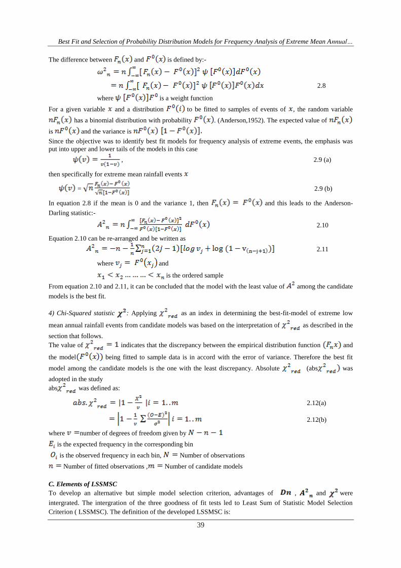
Best Fit and Selection of Probability Distribution Models for Frequency Analysis of Extreme Mean Annualhellip
39
The difference between and is defined by-
28
where is a weight function
For a given variable and a distribution to be fitted to samples of events of the random variable
has a binomial distribution with probability (Anderson1952) The expected value of
is and the variance is
Since the objective was to identify best fit models for frequency analysis of extreme events the emphasis was
put into upper and lower tails of the models in this case
29 (a)
then specifically for extreme mean rainfall events
= 29 (b)
In equation 28 if the mean is 0 and the variance 1 then and this leads to the Anderson-
Darling statistic-
210
Equation 210 can be re-arranged and be written as
211
where and
is the ordered sample
From equation 210 and 211 it can be concluded that the model with the least value of among the candidate
models is the best fit
4) Chi-Squared statistic Applying as an index in determining the best-fit-model of extreme low
mean annual rainfall events from candidate models was based on the interpretation of as described in the
section that follows
The value of indicates that the discrepancy between the empirical distribution function and
the model being fitted to sample data is in accord with the error of variance Therefore the best fit
model among the candidate models is the one with the least discrepancy Absolute (abs was
adopted in the study
abs was defined as
212(a)
212(b)
where number of degrees of freedom given by
is the expected frequency in the corresponding bin
is the observed frequency in each bin Number of observations
Number of fitted observations Number of candidate models
C Elements of LSSMSC
To develop an alternative but simple model selection criterion advantages of and were
intergrated The intergration of the three goodness of fit tests led to Least Sum of Statistic Model Selection
Criterion ( LSSMSC) The definition of the developed LSSMSC is
Best Fit and Selection of Probability Distribution Models for Frequency Analysis of Extreme Mean Annualhellip
40
213
where Kolomogrov-Smirnov statistic
Anderson-Darling statistic
Absolute reduced Chi-Square
= number of models
D Application of CMIC and LSSMIC
The developed CMIC and LSSMSC criteria were applied in Easy fit v55 software to identify candidate
and best fit models for the frequency analysis of the extreme mean annual events Mean annual rainfall data for
the period 1920-2004 for each of the 8 rainfall zones was obtained from Water Research Commission Pretoria
Easy fit V55 was chosen for this study because of the following features (mathwave2011)
1) It supports more than 50 continuous and discrete probability distribution functions
2) It has powerful automated fitting model combined with flexible manual fitting capabilities
3) It carries out goodness of fit tests
4) It has capability of generating random numbers
5) It is easily applied to user interface
6) There is comprehensive technical assistance from the developers (Mathwave2011)
Other scientific features which make Easy Fit V55 include
o It can be applied to analyze large data sets (up to 250000 data points)
o It includes application of advanced distributions to improve the validity of probability distribution
functions
o It can be applied to calculate descriptive statistics
o It organizes data and analyzes results into project files
1) Application of points below threshold (PBT) Model Points below threshold (PBT) model was applied to
identify extreme low mean annual rainfall events for each of the 8 rainfall zones For each of the 8 rainfall
zones the mean of mean annual rainfall values for the period 1920-2004 was chosen as the threshold for that
particular rainfall zone The mean rainfall events less than the threshold formed the extreme low mean annual
rainfall events The mean of mean annual rainfall values of each rainfall zone was chosen as the threshold
because annual rainfall less than the mean leads to agricultural drought
E Development of QT-T models
Based on the identified best fit model for frequency analysis extreme low mean annual rainfall events
for each of the 8 rainfall zones QT-T models were developed The developed QT-T models were applied to
extrapolate and estimate extreme low mean annual rainfall events for return periods of 5 10 25 50 100 and
200 years for each of the 8 rainfall zones The methods of parameter estimations applied were methods of
moments and maximum likelihood
F Assessment of performance of CMIC and LSSMIC
The performance of CMIC and LSSMIC as candidate and best fit models for frequency analysis of
extreme mean annual rainfall events was carried out by applying probability-probability (P-P) in EasyFit 55
software EasyFit 55 software displays reference graphic plots The closeness of the candidate model plot to the
reference graphic plots was the mode of the assessment applied This was visual assessment
III RESULTS A Descriptive statistics of extreme low mean annual rainfall for 8 rainfall zones
The descriptive statistics of events of the 8 samples of extreme low mean annual rainfall are presented
in table II The descriptive statistics were applied in developing QT-T models for frequency analysis of the
extreme low annual rainfall events in each rainfall zone The skewness and excess kurtosis of each sample have
been applied in describing the symmetry and the peakedness of the frequency distributions of these samples
Best Fit and Selection of Probability Distribution Models for Frequency Analysis of Extreme Mean Annualhellip
41
Table II Descriptive statistics
Rainfall zones X3a1 X3a2 X3b X3c X3d1 X3d2 X3e X3f
Statistic Value Value Value Value Value Value Value Value
Sample Size 50 47 49 51 51 47 52 50
Range 3888 4103 502 5263 5939 5528 4926 5001
Mean 8549 8336 8296 8265 8289 809 809 8206
Variance 9692 1076 1261 1733 1562 1493 1655 1624
Std Deviation 9845 1037 1123 1316 125 1222 1286 1274
Coef of Variation 01152 01245 01354 01593 01508 0151 0159 01553
Std Error 1392 1513 1604 1843 175 1782 1784 1802
Skewness -0549 -0460 -0923 -1043 -114 -0865 -0764 -0694
Excess Kurtosis -0454 -0428 0569 0784 1944 0738 -0230 -0200
The skewness value of each of the 8 samples of extreme mean annual rainfall is less than zero ie
negative This means that the frequency distribution of events in each of these samples is left skewed Most of
the events are concentrated on the right of the mean with extreme events to the left The excess kurtosis value of
each of the 8 samples is less than 3 This means that the frequency distribution of each sample is platykurtic
with peak flatter and wider than that of normal distribution
B Initial candidate models
The results of applying CMIC to each of the 8 data samples of extreme low mean annual rainfall are
presented in table II To obtain these results method described in section B was applied The results showed that
all the 8 samples had similar candidate models presented in table IIThese candidate models are Beta
Generalised Extreme Value Generalised Logistic Generalised Pareto Johson SB Kamaraswany Log-Pearson
3 Piet Phased Bi- Webull Power function Recipricol Triangular Uniform and Wakeby
C Final candidate models
Step 2 of the CMIC described in section B was applied to sets of the initial identified candidate models
given in table II The results are presented in tables 33-35 The results showed that the final candidate models
for frequency analysis of extreme low mean annual rainfall events in each of the 8 rainfall zones were
Generalised Logistic (GL) Log-Pearson 3 (LP3) and Generalised Extreme Value (GEV) The CDFs and PDFs
of the identified candidate models are presented in table VII
Generalised Logistic Log-Pearson 3 and Generalised Extreme Value frequency analysis models were
identified as the final candidate models because none of these models was rejected at significance levels
0201 002 and 001 in the three goodness of fit test in any of the 8 samples of extreme low mean rainfall
events The results of goodness of fit tests are presented in tables IV-VI
Table III The identified initial candidate models
Distribution Kolmogorov
Smirnov
Anderson
Darling ( A2n)
Chi-Squared
)
Statistic Rank Statistic Rank Statistic Rank
Beta 00731 3 2155 7 256 5
Gen Extreme Value 00795 5 02345 3 2898 7
Gen Logistic 0102 10 05311 5 2863 6
Gen Pareto 00894 7 1149 12 NA
Johnson SB 00704 1 0168 1 418 9
Kumaraswamy 00718 2 2153 6 256 4
Log-Pearson 3 00931 8 03815 4 127 1
Pert 01366 12 4782 10 64 10
Phased Bi-Exponential 09992 15 5126 15 NA
Phased Bi-Weibull 04529 14 5226 14 NA
Power Function 00871 6 2216 8 178 2
Reciprocal 02855 13 987 11 1618 11
Triangular 01047 11 2431 9 232 3
Uniform 00954 9 1501 13 NA
Wakeby 00748 4 02058 2 3774 8
Best Fit and Selection of Probability Distribution Models for Frequency Analysis of Extreme Mean Annualhellip
42
Tables IV-VI Identified final candidate models
Table IV Generalised Extreme Value distribution
Gen Extreme Value
Kolmogorov-Smirnov ( )
Sample Size
Statistic
P-Value
Rank
47
00815
08886
1
02 01 005 002 001
Critical Value 0153 01748 01942 02172 0233
Reject No No No No No
Anderson-Darling (A2
n )
Sample Size
Statistic
Rank
47
034
1
02 01 005 002 001
Critical Value 1375 1929 2502 3289 3907
Reject No No No No No
Chi-Squared ( )
Deg of freedom
Statistic
P-Value
Rank
4
417
03836
2
02 01 005 002 001
Critical Value 5989 7779 9488 1167 1328
Reject No No No No No
Table V Generalised Logistics distribution
Gen Logistic
Kolmogorov-Smirnov (
Sample Size
Statistic
P-Value
Rank
47
01055
06343
3
02 01 005 002 001
Critical Value 0153 01748 01942 02172 0233
Reject No No No No No
Anderson-Darling (A2
n)
Sample Size
Statistic
Rank
47
05878
3
02 01 005 002 001
Critical Value 1375 1929 2502 3289 3907
Reject No No No No No
Chi-Squared (
Deg of freedom
Statistic
P-Value
Rank
4
3292
05102
1
02 01 005 002 001
Critical Value 5989 7779 9488 1167 1328
Reject No No No No No
Best Fit and Selection of Probability Distribution Models for Frequency Analysis of Extreme Mean Annualhellip
43
Table VI Log-Pearson distribution
Log-Pearson 3
Kolmogorov-Smirnov ( )
Sample Size
Statistic
P-Value
Rank
47
00899
08093
2
02 01 005 002 001
Critical Value 0153 01748 01942 02172 0233
Reject No No No No No
Anderson-Darling ( A2n)
Sample Size
Statistic
Rank
47
03954
2
02 01 005 002 001
Critical Value 1375 1929 2502 3289 3907
Reject No No No No No
Chi-Squared (
Deg of freedom
Statistic
P-Value
Rank
5
433
05029
3
02 01 005 002 001
Critical Value 7289 9236 1107 1339 1509
Reject No No No No No
Table VII Candidate models for modeling the distribution of extreme low mean annual rainfall events in 8
rainfall zones in Sabie river catchment
Distribution CDF or PDF Domain
Generalized Extreme
Value
Generalized Logistics
Log-Pearson 3
D Results of identification of best-fit models for frequency analysis of extreme low mean annual rainfall
events in Sabie river catchment
The best fit models for frequency analysis of extreme low mean annual rainfall events in 8 rainfall
zones in Sabie river catchment are presented in tables VII-XV The summary of the results of the best fit model
identification is presented in table XVI
Table VIII Best fit model Zone X3 a1
Distribution Kolmogorov
Smirnov
Anderson
Darling
A2
n
Chi-Squared
Abs(1- LSSMIC Best fit
Statistic Statistic Statistic
Gen Extreme Value 0079 0234 2898 1898 2211
Gen Logistic 0102 0531 2863 1863 2496
Log-Pearson 3 0093 0381 1270 0270 0744 X
Best Fit and Selection of Probability Distribution Models for Frequency Analysis of Extreme Mean Annualhellip
44
Table IX Best fit model Zone X3a2
Distribution Kolmogorov
Smirnov
Anderson
Darling
A2n
Chi-Squared (
Abs (1- LSSMIC Best fit
Statistic Statistic Statistic
Gen Logistic 0105 0587 3292 2292 2984 x
Gen Extreme Value 0081 0340 4170 3170 3591
Log-Pearson 3 0089 0395 4330 3330 3814
Table X Best fit model Zone X3b
Distribution Kolmogorov
Smirnov
Anderson
Darling A2n
Chi-Squared ( Abs (1- LSSMIC Best fit
Statistic Statistic Statistic
Gen Logistic 0073 0302 2653 1653 2028 x
Johnson SB 0089 0241 5127 4127 4457
Log-Pearson 3 0077 0273 7055 6055 6405
Table XI Best fit model Zone X31c
Distribution Kolmogorov
Smirnov
Anderson
Darling(
A2n)
Chi-
Squared
(
Abs (1-
LSSMIC Best
fit
Statistic Statistic Statistic
Gen Extreme Value 0042 0133 0350 0649 0824
Log-Pearson 3 0059 0248 0866 0133 0440 x
Gen Logistic 0069 0286 2065 1065 1420
Table XII Best fit model Zone X3d1
Distribution Kolmogorov
Smirnov (
Anderson
Darling
(A2
n)
Chi-Squared
(
Abs ( 1- LSSMIC Best fit
Statistic Statistic Statistic
Wakeby 0088 1362 3262 2262 3712
Gen Logistic 0106 0516 3950 2950 3572 x
Gen Extreme Value 0097 0446 5923 4923 5466
Table XII Best fit model Zone X3d2
Distribution Kolmogorov
Smirnov
Anderson
Darling
(A2n)
Chi-Squared
(
Abs (1- LSSMIC Best fit
Statistic Statistic Statistic
Gen Extreme Value 0054 0118 0799 0201 0373 x
Gen Logistic 0082 0191 1334 0334 0607
Log-Pearson 3 0055 0124 1553 0553 0732
Table XIV Best fit model Zone X3e
Distribution Kolmogorov
Smirnov
Anderson
Darling
A2
n
Chi-Squared
(
Abs(1- LSSMIC Best fit
Statistic Statistic Statistic
Gen Extreme Value 0088 0461 2029 1029 1578 X
Gen Logistic 0107 0771 3415 2415 3293
Log-Pearson 3 0125 0770 3432 2432 3327
Best Fit and Selection of Probability Distribution Models for Frequency Analysis of Extreme Mean Annualhellip
45
Table XV Best fit model Zone X3f
Distribution Kolmogorov
Smirnov
Anderson
Darling (
A2n)
Chi-
Squared
(
Abs ( 1-
LSSMIC Best
fit
Statistic Statistic Statistic
Log-Pearson 3 0072 0401 1244 0244 0717 X
Gen Extreme Value 0057 0265 1843 0843 1165
Gen Logistic 0092 0560 4527 3527 4179
Table XVI Summary of best fit model identification results
Best fit model
Log-Pearson 3
Rainfall zones
3 375
Generalized Logistic 3 375
Generalized Extreme Value 2 25
Totals 8 100
Log- Pearson 3 and Generalised Logistic models each was the best fit models for frequency analysis of
extreme low mean annual rainfall events in 3 rainfall zones Generalised extreme value model was the best fit in
2 rainfall zones The results shows that there no single model which is the best fit for frequency analysis of all
low mean annual rainfall events in Sabie river catchment
Table XVII Best fit and QT-T models for frequency analysis of extreme low mean annual rainfall events
Rainfall
zone
Best fit
model
QT-T model
X3a1 LP 3
X3a2 GL
X3b GL
X3c LP 3
X3d1 GL
X3d2 GEV
X3e GEV
X3f LP 3
E Results of frequency analysis of extreme low mean annual rainfall events in 8 rainfall zones in water
deficit catchments in South Africa
The results of frequency analysis of extreme low mean annual rainfall events in the 8 zones of water
deficit catchments in South Africa are presented in table XVIII
Best Fit and Selection of Probability Distribution Models for Frequency Analysis of Extreme Mean Annualhellip
46
Table XVIII Recurrence intervals in years of extreme low mean annual rainfall events
F How CMIC and LSSMIC address common limitations of model identification criteria
General Information Criteria (GIC) can be expressed as
31
where is the measure lack of fit by model
is the dimension of defined as the number of free parameter under model
is the penalty for complexity of the model (Parsimony)
may depend on effective sample size and dimension of (free parameters)
Addressing of limitations cited by Jiang (2014) by developing CMIC and LSSMIC was based on Equation 31
Emanating from this work and based on the results obtained thereof following can be considered with respect to
the previous cited limitations with the current model selection criteria
Limitation of effective sample size
In the case where the sample size is not equal to sample points this limitation is addressed by identifying
candidate models and best models based on characteristic of sample probability tail events and hypothesis
significance levels Sample distribution tail shape and not size is applied In so doing the effect of sample size is
eliminated Kolomogrov-Smirnov goodness-of-fit index is a component of LSSMIC This index is generally not
influenced by the possible inequality of sample size against the sample points especially in case of correlations
Limitation due to dimension of the model (parameters)
For practical purposes as illustrated in previous sections the Anderson-Darling goodness-of-fit index has been
adjusted to address the complexity of the problem (Refer to Equation 211) Chi-Squared goodness-of-fit was
also adjusted to absolute index to address the limitation of dimension of the model (Refer to Equation 212(a))
Over and under parameter fitting limitation was also addressed in developing of absolute Chi-Squared index
(Refer to Equation 212(b) In this procedure parsimony was also addressed Both Anderson-Darling and Chi-
Squared indices are elements in LSSMIC
Limitation of ambiguity
Determination of LSSMIC index results into specific numbers which in turn reduces ambiguity A special case
is when parameters shape or scale of Wakeby model is equal to zero In that case Wakeby and Generalized
Pareto statistics are equal and if are the least then the two models are taken as the best fit
Rainfall
zone
Best-
fit
Mathematical model
Recurrence interval in years
5 10 25 50 100 200
X3a1 LP3
7706 7318 6984 6776 6624 647 6
X3a2 GL
9912 9855 9790 9749 9708 9671
X3b GL
9362 9030 8691 8484 8306 8152
X3c LP3 7167 6823 6678 6415 6290 6154
X3d1 GL
9260 8891 8459 8200 7973 7772
X3d2 GEV
8751 8417 8160 8044 7968 7899
X3e GEV
8627 8317 8093 7999 7940 7903
X3f LP3
7120 6801 6307 6045 5912 5782
Best Fit and Selection of Probability Distribution Models for Frequency Analysis of Extreme Mean Annualhellip
47
Limitation of Criterion of Optimality
CMIC and LSSMIC have been developed in such a way that other parameters can be included This approach
ensures that technical and social parameters or variables can be included when needed In this particular case
peaks under threshold models have been included This could practically be assigned to the demand for water
resources needed at catchment level
Limitation of small sample and extreme events
This limitation is deemed to be solved by including Anderson-Darling and Kolomogrov-Smirnov in LSSMIC as
both cater for small sample and extreme events scenarios
IV CONCLUSION The main objective of this study was to develop two model identification criteria for frequency
analysis of extreme low mean rainfall events in water deficit catchments in South Africa The two model
selection criteria which were developed are
1 Candidate Model Identification Criterion (CM1C) for identifying candidate models
2 Least Sum of Statistics Model Identification Criterion ( LSSM1C) for identifying the best fit models for
frequency analysis of the extreme low mean annual rainfall events from the identified candidate models
The two developed criteria were applied to identify candidate models and best fit models for frequency analyses
of the extreme low mean annual rainfall events in 8 rainfall zones in Sabie river catchment Results obtained
showed that there no single probability distribution function is the best fit for all the 8 rainfall zones (table XVI)
Log-Pearson 3 (LP3) probability distribution function has been recommended for design hydro-
meteorological events mostly flood and drought in South Africa (Alexander 1990 2001) From the results of
this study Log-Pearson 3 may not be the only best fit model for frequency analyses of extreme hydro-
meteorological events in South Africa It is therefore important to carry out model identification processes to
identify best fit model for the specific required frequency analysis
Probability-Probability (P-P) plots were applied to evaluate the performance of CMIC and LSSMISC
The plots showed that CMIC and LSSMIC performed fairly well Although the Probability-Probability (P-P)
plot results cannot be considered completely conclusive CMIC and LSSMSC criteria make useful tools as
model selection method for frequency analysis of extreme mean annual rainfall events
ACKNOWLEDGEMENT The study has been supported by the Provincial Dept of Agriculture Rural Development Land and
Environmental Affairs Mpumalanga Provincial Government South Africa
REFERENCES [1] Akaike H 1974`` A new look at the statistical model identificationrsquorsquoIEEE Transaction on automatic
control vol 6 pp 716-725
[2] Alexander WJR 1990 Flood Hydrology for Southern Africa SANCOLD Pretoria RSA
[3] Alexander WJR 2001 Flood Risk Reduction Measures University of Pretoria Pretoria RSA
[4] Alexander WJR 2002a The standard design flood Journal of the South Africa Institution of Civil
[5] Engineers 44 (1)26-31
[6] Anderson TW Darling DA 1952 Asymptotic theory of certain goodness-of-fit criteria based on
[7] stochastic processes AnnMatStat 23 193-212
[8] AndersonD R and Burnham K P 2002 Avoiding pitfalls when using information-theoretic
methods Journal of wildlife management 66(3) 912-918
[9] Beven K J 2000 Rain-Run-off modeling The Primer John Wiley and sons Chichester UK 360
360pp
[10] Bobee B and Rasmussen P F 1995 Recent advances in flood frequency analysis Reviews of
Geophysics supplement July 1111-1116
[11] Bodini A and Cossu Q A 2010 Vulnerability assessment of Central-East Sardinia ( Italy) to
extreme rainfall events Journal of Natural hazards and Earth systems sciences 10 Pp 61-77
[12] Claeskens G Hjort NL 2003 The focused Information Criterion Journal of the American statistical
[13] Association 98 900-916
[14] FeyenHMJ 1970 Identification of run-off processes in catchments with a small scale topograph
[15] Furrer E M and Katz R W 2008 ``Improving the simulation of extreme precipitation events by
stochastic weather generatorsrsquorsquo Water Resources Research 44 W 12439doi 10292008 WR 007316
2008
[16] Gericke OJ 2010 Evaluation of the SDF method using a customized Design Flood Estimation Tool
University of Stellenbosch Stellenbosch South Africa 480 pp
Best Fit and Selection of Probability Distribution Models for Frequency Analysis of Extreme Mean Annualhellip
48
[17] Gorgens A H M Joint Peak- Volume ( JPV) Design Flood Hydrographs for South Africa WRC
Report 1420307 Water Research Commission Pretoria South Africa
[18] Gorgens A H M LysonsS Hayes L Makhabana M and Maluleke D 2007 Modernised South
African Design Floo Pro actce in the context of Dam safety WRC Report 1420 2 07 Water
Research omission Pretoria South Africa
[19] Goswani P and Ramesh K V 2007 Extreme rainfall events Vulnerability Analysis for Disaster
Management and Observation Systems Design Research Report CSIR PP21
[20] Hernandez A R P Balling R C Jr and Barber-Matinez 2009 Comparative analysis of indices of
extreme rainfall events Variation and trend from Southern Mexico Journal de Atmosfera 2 pages 219-
228
[21] Hosking JRM 1990 L-moments Analysis and estimation of distribution using Linear combinations
of
[22] order statistics Journal of the Royal statistics society Series B 52 105-124
[23] Hosking JRM Wallis JR Wood EF 1985 Estimation of the generalized extreme-value
distribution
[24] by the method of probability-weighted moments Technimetrics 27 (3) pp 251-261
[25] Hjort NL Claeskens G 2003 Rejoinder to the focused
[26] Jiang J 2014 The fence method Advances in statistics Volume 2014 Article ID 38081
[27] Kidson R Richards KS Carling PA 2005 Reconstructing the Ca-100 year flood in Northern
[28] Thailand Geomorphology 70 (2-4) 279-595
[29] Kottegoda NT Rosso R 1998 Statistics Probability and Reliability for Civil and Environmental
[30] Engineers McGrawHill New York
[31] Laio etal 2009 Model selection techniques for the frequency analysis of hydrological extremes
water
[32] Research Vol45 W07416
[33] Laio F 2004 Cramer-Von Mises and Anderson-Darling goodness-of-fit tests for extreme value
[34] distributions with unknown parameters Water Resources Research 40 W09308
[35] doi1010292004WR003204
[36] Mathwave(2011) httpwwwmathwavecom
[37] Mallows CL 1995 Some comments on Cp Technimetrics 37 362-372
[38] Mallows CL 1973 Some comments on Cp Technimetrics 15 661-675
[39] Meiz R and Bloschl G 2004 Regionaliisation of catchment model parameters J Hydrol 287 pp 95-
123
[40] Mkhandi SH Kachroo RK Gunasekara TAG 2000 Flood frequency analysis of Southern
Africa
[41] II Identification of regional distributions Hydrological Sciences Journal 45(3)449-464
[42] Mutua FM 1994 The use of the Akaike Information Criterion in the identification of an optimum
flood
[43] frequency model Hydro SciJ39 (3) 235-244
[44] Salami A W ( 2004) Prediction of the annual flow regime along Asa River using probability
distribution models AMSE periodicals Lyon France Modeling c-2004 65 (2) 41-56 ( httpamse-
modelingorgcontentamse 2004 htm)
[45] Schwarz G 1978 Estimating the dimension of a model Annals stat 6 461-464
[46] Schulze RE 1989 Non-stationary catchment responses and other problems in determing flood
series A case for a simulation modeling approach In Kienzle S W Maaren H (Eds) Proceedings
of the Fourth South African National Hyrological Symposium SANCIAHS Pretoria RSA pp 135-157
[47] ShamirE 2005 2004Application of temporal streamflow descriptors in hydrologic model parameter
estimationWater Resource Research 41 doi 10 10292004 WR 003409 SSN 0043-1397
[48] Shao J Sitter RR 1996 Bootstrip for imprinted Survey data Journal of the American statistical
[49] Association 93 819-831
[50] Smithers JC Schulze RE 2001 Design runoff estimation A review with reference to practices in
[51] South Africa Proceedings of Tenth South Africa National Hydrology Symposium 26-28 September
[52] 2001 School of BEEH University of Natal Pietermaritzburg RSA
[53] Smithers JC Schulze RE 2003 Design rainfall and flood estimation in South AfricaWRC Report
No
[54] 10600103 Water Research Commission Pretoria RSA
[55] Stedinger JR Vogel RM Foufoula E 1993 Frequency analysis of extreme events in Handbook
of
[56] Hydrology DR McGrawHill chap 18 66pp
Best Fit and Selection of Probability Distribution Models for Frequency Analysis of Extreme Mean Annualhellip
49
[57] Stedinger JR 1980 Fitting log normal distribution to hydrologic data Water Resource research
16(3)
[58] pp 481-490
[59] Stephens MA 1976 Asymptotic results for goodness-of-fit statistics with unknown parameters Ann
[60] Stat Vol 4 357-369
[61] Van der Linde A 2005 DIC in variable selection statistical Neerlandica 59 45-56
[62] Van der Linde A 2004 DIC in variable selection Technical report Institute of statistics University of
[63] Bremen httpwwwmathuni-bremende$simsard1downloadpapersvarse12pdf
[64] Wellner JA 1977 Aglirenko-Cantelli Theorem and strong laws of large numbers for function of
order
[65] statistics The annual of statistics vol5 number 3 1977 473-480
[66] Wilks DS 1998 Multi-site generalization of daily stochastic precipitation model J Hydro 210 178-
191
[67] Willens P Olsson J Ambjerg_Nielsen BeechamS Pathirana A BulowGregersen MadsenH and
Nguyen VTV 2007 Impact of climate change on rainfall extreme and urban drainage systems pp19-
20
[68] WMO- World Meteorological organization 1988 Analysing long Time Series of Hydrological data
with respect of climat variability WCAP-No 3 WMO-TD No 224
[69] WMO- World Meteorological organization 2009 Guidelines on Analysis of extremes in a changing
climate in support of informed decisions for adaptations WCDMP-No 72 WMO-TD No 1500
[70] Yua-Ping Xu Booij Martin J Tong Yang_Bin 2010 Uncertainity analysis in statistical modeling of
extreme hydrological events
[71] Yue S and Wang 2004 The Mann-Kendall test modified by effective sample size to detect trend in
serially correlated hydrological series Journal of Water Resources Management 18 Pages 201-218
Appendix A Probability-Probability (P-P) plots for extreme low mean rainfall events for the
8 rainfall zones
P-P Plot Zone X3a1
Gen Extreme Value Gen Logistic Log-Pearson 3
P (Empirical)
1090807060504030201
P (
Mo
de
l)
1
09
08
07
06
05
04
03
02
01
0
Fig 1 P-P plot Zone x3a1 Extreme mean annual rainfall events
Best Fit and Selection of Probability Distribution Models for Frequency Analysis of Extreme Mean Annualhellip
50
P-P Plot Zone x3a2
Gen Extreme Value Gen Logistic Log-Pearson 3
P (Empirical)
1090807060504030201
P (
Mo
de
l)
1
09
08
07
06
05
04
03
02
01
0
Fig 2 P-P plot Zone x3a2 Extreme mean annual rainfall events
P-P Plot Zone x3b
Gen Logistic Log-Pearson 3 Wakeby
P (Empirical)
1090807060504030201
P (
Model)
1
09
08
07
06
05
04
03
02
01
0
Fig 3 P-P plot Zone x3b Extreme mean annual rainfall events
Best Fit and Selection of Probability Distribution Models for Frequency Analysis of Extreme Mean Annualhellip
51
P-P Plot Zone x3c
Gen Extreme Value Gen Logistic Log-Pearson 3
P (Empirical)
10908070605040302010
P (
Model)
1
09
08
07
06
05
04
03
02
01
0
Fig4 P-P plot Zone x3c Extreme mean annual rainfall events
P-P Plot Zone x3d1
Gen Extreme Value Gen Logistic Wakeby
P (Empirical)
10908070605040302010
P (
Model)
1
09
08
07
06
05
04
03
02
01
0
Fig 5 P-P plot Zone x3d1 Extreme mean annual rainfall events
Best Fit and Selection of Probability Distribution Models for Frequency Analysis of Extreme Mean Annualhellip
52
P-P Plot Zone x3d2
Gen Extreme Value Gen Logistic Log-Pearson 3
P (Empirical)
1090807060504030201
P (
Model)
1
09
08
07
06
05
04
03
02
01
0
FIG 6 P-P plot Zone x3d2 Extreme mean annual rainfall events
P-P Plot Zone x3e
Gen Extreme Value Gen Logistic Log-Pearson 3
P (Empirical)
1080604020
P (
Model)
1
09
08
07
06
05
04
03
02
01
0
Fig 7 P-P plot Zone x3e Extreme mean annual rainfall events
Best Fit and Selection of Probability Distribution Models for Frequency Analysis of Extreme Mean Annualhellip
53
P-P Plot Zone x3f
Gen Extreme Value Gen Logistic Log-Pearson 3
P (Empirical)
1090807060504030201
P (
Mo
de
l)
1
09
08
07
06
05
04
03
02
01
0
Fig8 P-P plot Zone x3f Extreme mean annual rainfall events
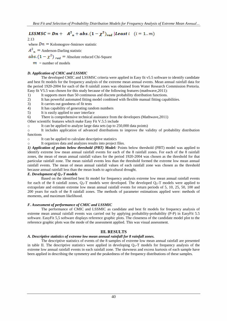
Best Fit and Selection of Probability Distribution Models for Frequency Analysis of Extreme Mean Annualhellip
41
Table II Descriptive statistics
Rainfall zones X3a1 X3a2 X3b X3c X3d1 X3d2 X3e X3f
Statistic Value Value Value Value Value Value Value Value
Sample Size 50 47 49 51 51 47 52 50
Range 3888 4103 502 5263 5939 5528 4926 5001
Mean 8549 8336 8296 8265 8289 809 809 8206
Variance 9692 1076 1261 1733 1562 1493 1655 1624
Std Deviation 9845 1037 1123 1316 125 1222 1286 1274
Coef of Variation 01152 01245 01354 01593 01508 0151 0159 01553
Std Error 1392 1513 1604 1843 175 1782 1784 1802
Skewness -0549 -0460 -0923 -1043 -114 -0865 -0764 -0694
Excess Kurtosis -0454 -0428 0569 0784 1944 0738 -0230 -0200
The skewness value of each of the 8 samples of extreme mean annual rainfall is less than zero ie
negative This means that the frequency distribution of events in each of these samples is left skewed Most of
the events are concentrated on the right of the mean with extreme events to the left The excess kurtosis value of
each of the 8 samples is less than 3 This means that the frequency distribution of each sample is platykurtic
with peak flatter and wider than that of normal distribution
B Initial candidate models
The results of applying CMIC to each of the 8 data samples of extreme low mean annual rainfall are
presented in table II To obtain these results method described in section B was applied The results showed that
all the 8 samples had similar candidate models presented in table IIThese candidate models are Beta
Generalised Extreme Value Generalised Logistic Generalised Pareto Johson SB Kamaraswany Log-Pearson
3 Piet Phased Bi- Webull Power function Recipricol Triangular Uniform and Wakeby
C Final candidate models
Step 2 of the CMIC described in section B was applied to sets of the initial identified candidate models
given in table II The results are presented in tables 33-35 The results showed that the final candidate models
for frequency analysis of extreme low mean annual rainfall events in each of the 8 rainfall zones were
Generalised Logistic (GL) Log-Pearson 3 (LP3) and Generalised Extreme Value (GEV) The CDFs and PDFs
of the identified candidate models are presented in table VII
Generalised Logistic Log-Pearson 3 and Generalised Extreme Value frequency analysis models were
identified as the final candidate models because none of these models was rejected at significance levels
0201 002 and 001 in the three goodness of fit test in any of the 8 samples of extreme low mean rainfall
events The results of goodness of fit tests are presented in tables IV-VI
Table III The identified initial candidate models
Distribution Kolmogorov
Smirnov
Anderson
Darling ( A2n)
Chi-Squared
)
Statistic Rank Statistic Rank Statistic Rank
Beta 00731 3 2155 7 256 5
Gen Extreme Value 00795 5 02345 3 2898 7
Gen Logistic 0102 10 05311 5 2863 6
Gen Pareto 00894 7 1149 12 NA
Johnson SB 00704 1 0168 1 418 9
Kumaraswamy 00718 2 2153 6 256 4
Log-Pearson 3 00931 8 03815 4 127 1
Pert 01366 12 4782 10 64 10
Phased Bi-Exponential 09992 15 5126 15 NA
Phased Bi-Weibull 04529 14 5226 14 NA
Power Function 00871 6 2216 8 178 2
Reciprocal 02855 13 987 11 1618 11
Triangular 01047 11 2431 9 232 3
Uniform 00954 9 1501 13 NA
Wakeby 00748 4 02058 2 3774 8
Best Fit and Selection of Probability Distribution Models for Frequency Analysis of Extreme Mean Annualhellip
42
Tables IV-VI Identified final candidate models
Table IV Generalised Extreme Value distribution
Gen Extreme Value
Kolmogorov-Smirnov ( )
Sample Size
Statistic
P-Value
Rank
47
00815
08886
1
02 01 005 002 001
Critical Value 0153 01748 01942 02172 0233
Reject No No No No No
Anderson-Darling (A2
n )
Sample Size
Statistic
Rank
47
034
1
02 01 005 002 001
Critical Value 1375 1929 2502 3289 3907
Reject No No No No No
Chi-Squared ( )
Deg of freedom
Statistic
P-Value
Rank
4
417
03836
2
02 01 005 002 001
Critical Value 5989 7779 9488 1167 1328
Reject No No No No No
Table V Generalised Logistics distribution
Gen Logistic
Kolmogorov-Smirnov (
Sample Size
Statistic
P-Value
Rank
47
01055
06343
3
02 01 005 002 001
Critical Value 0153 01748 01942 02172 0233
Reject No No No No No
Anderson-Darling (A2
n)
Sample Size
Statistic
Rank
47
05878
3
02 01 005 002 001
Critical Value 1375 1929 2502 3289 3907
Reject No No No No No
Chi-Squared (
Deg of freedom
Statistic
P-Value
Rank
4
3292
05102
1
02 01 005 002 001
Critical Value 5989 7779 9488 1167 1328
Reject No No No No No
Best Fit and Selection of Probability Distribution Models for Frequency Analysis of Extreme Mean Annualhellip
43
Table VI Log-Pearson distribution
Log-Pearson 3
Kolmogorov-Smirnov ( )
Sample Size
Statistic
P-Value
Rank
47
00899
08093
2
02 01 005 002 001
Critical Value 0153 01748 01942 02172 0233
Reject No No No No No
Anderson-Darling ( A2n)
Sample Size
Statistic
Rank
47
03954
2
02 01 005 002 001
Critical Value 1375 1929 2502 3289 3907
Reject No No No No No
Chi-Squared (
Deg of freedom
Statistic
P-Value
Rank
5
433
05029
3
02 01 005 002 001
Critical Value 7289 9236 1107 1339 1509
Reject No No No No No
Table VII Candidate models for modeling the distribution of extreme low mean annual rainfall events in 8
rainfall zones in Sabie river catchment
Distribution CDF or PDF Domain
Generalized Extreme
Value
Generalized Logistics
Log-Pearson 3
D Results of identification of best-fit models for frequency analysis of extreme low mean annual rainfall
events in Sabie river catchment
The best fit models for frequency analysis of extreme low mean annual rainfall events in 8 rainfall
zones in Sabie river catchment are presented in tables VII-XV The summary of the results of the best fit model
identification is presented in table XVI
Table VIII Best fit model Zone X3 a1
Distribution Kolmogorov
Smirnov
Anderson
Darling
A2
n
Chi-Squared
Abs(1- LSSMIC Best fit
Statistic Statistic Statistic
Gen Extreme Value 0079 0234 2898 1898 2211
Gen Logistic 0102 0531 2863 1863 2496
Log-Pearson 3 0093 0381 1270 0270 0744 X
Best Fit and Selection of Probability Distribution Models for Frequency Analysis of Extreme Mean Annualhellip
44
Table IX Best fit model Zone X3a2
Distribution Kolmogorov
Smirnov
Anderson
Darling
A2n
Chi-Squared (
Abs (1- LSSMIC Best fit
Statistic Statistic Statistic
Gen Logistic 0105 0587 3292 2292 2984 x
Gen Extreme Value 0081 0340 4170 3170 3591
Log-Pearson 3 0089 0395 4330 3330 3814
Table X Best fit model Zone X3b
Distribution Kolmogorov
Smirnov
Anderson
Darling A2n
Chi-Squared ( Abs (1- LSSMIC Best fit
Statistic Statistic Statistic
Gen Logistic 0073 0302 2653 1653 2028 x
Johnson SB 0089 0241 5127 4127 4457
Log-Pearson 3 0077 0273 7055 6055 6405
Table XI Best fit model Zone X31c
Distribution Kolmogorov
Smirnov
Anderson
Darling(
A2n)
Chi-
Squared
(
Abs (1-
LSSMIC Best
fit
Statistic Statistic Statistic
Gen Extreme Value 0042 0133 0350 0649 0824
Log-Pearson 3 0059 0248 0866 0133 0440 x
Gen Logistic 0069 0286 2065 1065 1420
Table XII Best fit model Zone X3d1
Distribution Kolmogorov
Smirnov (
Anderson
Darling
(A2
n)
Chi-Squared
(
Abs ( 1- LSSMIC Best fit
Statistic Statistic Statistic
Wakeby 0088 1362 3262 2262 3712
Gen Logistic 0106 0516 3950 2950 3572 x
Gen Extreme Value 0097 0446 5923 4923 5466
Table XII Best fit model Zone X3d2
Distribution Kolmogorov
Smirnov
Anderson
Darling
(A2n)
Chi-Squared
(
Abs (1- LSSMIC Best fit
Statistic Statistic Statistic
Gen Extreme Value 0054 0118 0799 0201 0373 x
Gen Logistic 0082 0191 1334 0334 0607
Log-Pearson 3 0055 0124 1553 0553 0732
Table XIV Best fit model Zone X3e
Distribution Kolmogorov
Smirnov
Anderson
Darling
A2
n
Chi-Squared
(
Abs(1- LSSMIC Best fit
Statistic Statistic Statistic
Gen Extreme Value 0088 0461 2029 1029 1578 X
Gen Logistic 0107 0771 3415 2415 3293
Log-Pearson 3 0125 0770 3432 2432 3327
Best Fit and Selection of Probability Distribution Models for Frequency Analysis of Extreme Mean Annualhellip
45
Table XV Best fit model Zone X3f
Distribution Kolmogorov
Smirnov
Anderson
Darling (
A2n)
Chi-
Squared
(
Abs ( 1-
LSSMIC Best
fit
Statistic Statistic Statistic
Log-Pearson 3 0072 0401 1244 0244 0717 X
Gen Extreme Value 0057 0265 1843 0843 1165
Gen Logistic 0092 0560 4527 3527 4179
Table XVI Summary of best fit model identification results
Best fit model
Log-Pearson 3
Rainfall zones
3 375
Generalized Logistic 3 375
Generalized Extreme Value 2 25
Totals 8 100
Log- Pearson 3 and Generalised Logistic models each was the best fit models for frequency analysis of
extreme low mean annual rainfall events in 3 rainfall zones Generalised extreme value model was the best fit in
2 rainfall zones The results shows that there no single model which is the best fit for frequency analysis of all
low mean annual rainfall events in Sabie river catchment
Table XVII Best fit and QT-T models for frequency analysis of extreme low mean annual rainfall events
Rainfall
zone
Best fit
model
QT-T model
X3a1 LP 3
X3a2 GL
X3b GL
X3c LP 3
X3d1 GL
X3d2 GEV
X3e GEV
X3f LP 3
E Results of frequency analysis of extreme low mean annual rainfall events in 8 rainfall zones in water
deficit catchments in South Africa
The results of frequency analysis of extreme low mean annual rainfall events in the 8 zones of water
deficit catchments in South Africa are presented in table XVIII
Best Fit and Selection of Probability Distribution Models for Frequency Analysis of Extreme Mean Annualhellip
46
Table XVIII Recurrence intervals in years of extreme low mean annual rainfall events
F How CMIC and LSSMIC address common limitations of model identification criteria
General Information Criteria (GIC) can be expressed as
31
where is the measure lack of fit by model
is the dimension of defined as the number of free parameter under model
is the penalty for complexity of the model (Parsimony)
may depend on effective sample size and dimension of (free parameters)
Addressing of limitations cited by Jiang (2014) by developing CMIC and LSSMIC was based on Equation 31
Emanating from this work and based on the results obtained thereof following can be considered with respect to
the previous cited limitations with the current model selection criteria
Limitation of effective sample size
In the case where the sample size is not equal to sample points this limitation is addressed by identifying
candidate models and best models based on characteristic of sample probability tail events and hypothesis
significance levels Sample distribution tail shape and not size is applied In so doing the effect of sample size is
eliminated Kolomogrov-Smirnov goodness-of-fit index is a component of LSSMIC This index is generally not
influenced by the possible inequality of sample size against the sample points especially in case of correlations
Limitation due to dimension of the model (parameters)
For practical purposes as illustrated in previous sections the Anderson-Darling goodness-of-fit index has been
adjusted to address the complexity of the problem (Refer to Equation 211) Chi-Squared goodness-of-fit was
also adjusted to absolute index to address the limitation of dimension of the model (Refer to Equation 212(a))
Over and under parameter fitting limitation was also addressed in developing of absolute Chi-Squared index
(Refer to Equation 212(b) In this procedure parsimony was also addressed Both Anderson-Darling and Chi-
Squared indices are elements in LSSMIC
Limitation of ambiguity
Determination of LSSMIC index results into specific numbers which in turn reduces ambiguity A special case
is when parameters shape or scale of Wakeby model is equal to zero In that case Wakeby and Generalized
Pareto statistics are equal and if are the least then the two models are taken as the best fit
Rainfall
zone
Best-
fit
Mathematical model
Recurrence interval in years
5 10 25 50 100 200
X3a1 LP3
7706 7318 6984 6776 6624 647 6
X3a2 GL
9912 9855 9790 9749 9708 9671
X3b GL
9362 9030 8691 8484 8306 8152
X3c LP3 7167 6823 6678 6415 6290 6154
X3d1 GL
9260 8891 8459 8200 7973 7772
X3d2 GEV
8751 8417 8160 8044 7968 7899
X3e GEV
8627 8317 8093 7999 7940 7903
X3f LP3
7120 6801 6307 6045 5912 5782
Best Fit and Selection of Probability Distribution Models for Frequency Analysis of Extreme Mean Annualhellip
47
Limitation of Criterion of Optimality
CMIC and LSSMIC have been developed in such a way that other parameters can be included This approach
ensures that technical and social parameters or variables can be included when needed In this particular case
peaks under threshold models have been included This could practically be assigned to the demand for water
resources needed at catchment level
Limitation of small sample and extreme events
This limitation is deemed to be solved by including Anderson-Darling and Kolomogrov-Smirnov in LSSMIC as
both cater for small sample and extreme events scenarios
IV CONCLUSION The main objective of this study was to develop two model identification criteria for frequency
analysis of extreme low mean rainfall events in water deficit catchments in South Africa The two model
selection criteria which were developed are
1 Candidate Model Identification Criterion (CM1C) for identifying candidate models
2 Least Sum of Statistics Model Identification Criterion ( LSSM1C) for identifying the best fit models for
frequency analysis of the extreme low mean annual rainfall events from the identified candidate models
The two developed criteria were applied to identify candidate models and best fit models for frequency analyses
of the extreme low mean annual rainfall events in 8 rainfall zones in Sabie river catchment Results obtained
showed that there no single probability distribution function is the best fit for all the 8 rainfall zones (table XVI)
Log-Pearson 3 (LP3) probability distribution function has been recommended for design hydro-
meteorological events mostly flood and drought in South Africa (Alexander 1990 2001) From the results of
this study Log-Pearson 3 may not be the only best fit model for frequency analyses of extreme hydro-
meteorological events in South Africa It is therefore important to carry out model identification processes to
identify best fit model for the specific required frequency analysis
Probability-Probability (P-P) plots were applied to evaluate the performance of CMIC and LSSMISC
The plots showed that CMIC and LSSMIC performed fairly well Although the Probability-Probability (P-P)
plot results cannot be considered completely conclusive CMIC and LSSMSC criteria make useful tools as
model selection method for frequency analysis of extreme mean annual rainfall events
ACKNOWLEDGEMENT The study has been supported by the Provincial Dept of Agriculture Rural Development Land and
Environmental Affairs Mpumalanga Provincial Government South Africa
REFERENCES [1] Akaike H 1974`` A new look at the statistical model identificationrsquorsquoIEEE Transaction on automatic
control vol 6 pp 716-725
[2] Alexander WJR 1990 Flood Hydrology for Southern Africa SANCOLD Pretoria RSA
[3] Alexander WJR 2001 Flood Risk Reduction Measures University of Pretoria Pretoria RSA
[4] Alexander WJR 2002a The standard design flood Journal of the South Africa Institution of Civil
[5] Engineers 44 (1)26-31
[6] Anderson TW Darling DA 1952 Asymptotic theory of certain goodness-of-fit criteria based on
[7] stochastic processes AnnMatStat 23 193-212
[8] AndersonD R and Burnham K P 2002 Avoiding pitfalls when using information-theoretic
methods Journal of wildlife management 66(3) 912-918
[9] Beven K J 2000 Rain-Run-off modeling The Primer John Wiley and sons Chichester UK 360
360pp
[10] Bobee B and Rasmussen P F 1995 Recent advances in flood frequency analysis Reviews of
Geophysics supplement July 1111-1116
[11] Bodini A and Cossu Q A 2010 Vulnerability assessment of Central-East Sardinia ( Italy) to
extreme rainfall events Journal of Natural hazards and Earth systems sciences 10 Pp 61-77
[12] Claeskens G Hjort NL 2003 The focused Information Criterion Journal of the American statistical
[13] Association 98 900-916
[14] FeyenHMJ 1970 Identification of run-off processes in catchments with a small scale topograph
[15] Furrer E M and Katz R W 2008 ``Improving the simulation of extreme precipitation events by
stochastic weather generatorsrsquorsquo Water Resources Research 44 W 12439doi 10292008 WR 007316
2008
[16] Gericke OJ 2010 Evaluation of the SDF method using a customized Design Flood Estimation Tool
University of Stellenbosch Stellenbosch South Africa 480 pp
Best Fit and Selection of Probability Distribution Models for Frequency Analysis of Extreme Mean Annualhellip
48
[17] Gorgens A H M Joint Peak- Volume ( JPV) Design Flood Hydrographs for South Africa WRC
Report 1420307 Water Research Commission Pretoria South Africa
[18] Gorgens A H M LysonsS Hayes L Makhabana M and Maluleke D 2007 Modernised South
African Design Floo Pro actce in the context of Dam safety WRC Report 1420 2 07 Water
Research omission Pretoria South Africa
[19] Goswani P and Ramesh K V 2007 Extreme rainfall events Vulnerability Analysis for Disaster
Management and Observation Systems Design Research Report CSIR PP21
[20] Hernandez A R P Balling R C Jr and Barber-Matinez 2009 Comparative analysis of indices of
extreme rainfall events Variation and trend from Southern Mexico Journal de Atmosfera 2 pages 219-
228
[21] Hosking JRM 1990 L-moments Analysis and estimation of distribution using Linear combinations
of
[22] order statistics Journal of the Royal statistics society Series B 52 105-124
[23] Hosking JRM Wallis JR Wood EF 1985 Estimation of the generalized extreme-value
distribution
[24] by the method of probability-weighted moments Technimetrics 27 (3) pp 251-261
[25] Hjort NL Claeskens G 2003 Rejoinder to the focused
[26] Jiang J 2014 The fence method Advances in statistics Volume 2014 Article ID 38081
[27] Kidson R Richards KS Carling PA 2005 Reconstructing the Ca-100 year flood in Northern
[28] Thailand Geomorphology 70 (2-4) 279-595
[29] Kottegoda NT Rosso R 1998 Statistics Probability and Reliability for Civil and Environmental
[30] Engineers McGrawHill New York
[31] Laio etal 2009 Model selection techniques for the frequency analysis of hydrological extremes
water
[32] Research Vol45 W07416
[33] Laio F 2004 Cramer-Von Mises and Anderson-Darling goodness-of-fit tests for extreme value
[34] distributions with unknown parameters Water Resources Research 40 W09308
[35] doi1010292004WR003204
[36] Mathwave(2011) httpwwwmathwavecom
[37] Mallows CL 1995 Some comments on Cp Technimetrics 37 362-372
[38] Mallows CL 1973 Some comments on Cp Technimetrics 15 661-675
[39] Meiz R and Bloschl G 2004 Regionaliisation of catchment model parameters J Hydrol 287 pp 95-
123
[40] Mkhandi SH Kachroo RK Gunasekara TAG 2000 Flood frequency analysis of Southern
Africa
[41] II Identification of regional distributions Hydrological Sciences Journal 45(3)449-464
[42] Mutua FM 1994 The use of the Akaike Information Criterion in the identification of an optimum
flood
[43] frequency model Hydro SciJ39 (3) 235-244
[44] Salami A W ( 2004) Prediction of the annual flow regime along Asa River using probability
distribution models AMSE periodicals Lyon France Modeling c-2004 65 (2) 41-56 ( httpamse-
modelingorgcontentamse 2004 htm)
[45] Schwarz G 1978 Estimating the dimension of a model Annals stat 6 461-464
[46] Schulze RE 1989 Non-stationary catchment responses and other problems in determing flood
series A case for a simulation modeling approach In Kienzle S W Maaren H (Eds) Proceedings
of the Fourth South African National Hyrological Symposium SANCIAHS Pretoria RSA pp 135-157
[47] ShamirE 2005 2004Application of temporal streamflow descriptors in hydrologic model parameter
estimationWater Resource Research 41 doi 10 10292004 WR 003409 SSN 0043-1397
[48] Shao J Sitter RR 1996 Bootstrip for imprinted Survey data Journal of the American statistical
[49] Association 93 819-831
[50] Smithers JC Schulze RE 2001 Design runoff estimation A review with reference to practices in
[51] South Africa Proceedings of Tenth South Africa National Hydrology Symposium 26-28 September
[52] 2001 School of BEEH University of Natal Pietermaritzburg RSA
[53] Smithers JC Schulze RE 2003 Design rainfall and flood estimation in South AfricaWRC Report
No
[54] 10600103 Water Research Commission Pretoria RSA
[55] Stedinger JR Vogel RM Foufoula E 1993 Frequency analysis of extreme events in Handbook
of
[56] Hydrology DR McGrawHill chap 18 66pp
Best Fit and Selection of Probability Distribution Models for Frequency Analysis of Extreme Mean Annualhellip
49
[57] Stedinger JR 1980 Fitting log normal distribution to hydrologic data Water Resource research
16(3)
[58] pp 481-490
[59] Stephens MA 1976 Asymptotic results for goodness-of-fit statistics with unknown parameters Ann
[60] Stat Vol 4 357-369
[61] Van der Linde A 2005 DIC in variable selection statistical Neerlandica 59 45-56
[62] Van der Linde A 2004 DIC in variable selection Technical report Institute of statistics University of
[63] Bremen httpwwwmathuni-bremende$simsard1downloadpapersvarse12pdf
[64] Wellner JA 1977 Aglirenko-Cantelli Theorem and strong laws of large numbers for function of
order
[65] statistics The annual of statistics vol5 number 3 1977 473-480
[66] Wilks DS 1998 Multi-site generalization of daily stochastic precipitation model J Hydro 210 178-
191
[67] Willens P Olsson J Ambjerg_Nielsen BeechamS Pathirana A BulowGregersen MadsenH and
Nguyen VTV 2007 Impact of climate change on rainfall extreme and urban drainage systems pp19-
20
[68] WMO- World Meteorological organization 1988 Analysing long Time Series of Hydrological data
with respect of climat variability WCAP-No 3 WMO-TD No 224
[69] WMO- World Meteorological organization 2009 Guidelines on Analysis of extremes in a changing
climate in support of informed decisions for adaptations WCDMP-No 72 WMO-TD No 1500
[70] Yua-Ping Xu Booij Martin J Tong Yang_Bin 2010 Uncertainity analysis in statistical modeling of
extreme hydrological events
[71] Yue S and Wang 2004 The Mann-Kendall test modified by effective sample size to detect trend in
serially correlated hydrological series Journal of Water Resources Management 18 Pages 201-218
Appendix A Probability-Probability (P-P) plots for extreme low mean rainfall events for the
8 rainfall zones
P-P Plot Zone X3a1
Gen Extreme Value Gen Logistic Log-Pearson 3
P (Empirical)
1090807060504030201
P (
Mo
de
l)
1
09
08
07
06
05
04
03
02
01
0
Fig 1 P-P plot Zone x3a1 Extreme mean annual rainfall events
Best Fit and Selection of Probability Distribution Models for Frequency Analysis of Extreme Mean Annualhellip
50
P-P Plot Zone x3a2
Gen Extreme Value Gen Logistic Log-Pearson 3
P (Empirical)
1090807060504030201
P (
Mo
de
l)
1
09
08
07
06
05
04
03
02
01
0
Fig 2 P-P plot Zone x3a2 Extreme mean annual rainfall events
P-P Plot Zone x3b
Gen Logistic Log-Pearson 3 Wakeby
P (Empirical)
1090807060504030201
P (
Model)
1
09
08
07
06
05
04
03
02
01
0
Fig 3 P-P plot Zone x3b Extreme mean annual rainfall events
Best Fit and Selection of Probability Distribution Models for Frequency Analysis of Extreme Mean Annualhellip
51
P-P Plot Zone x3c
Gen Extreme Value Gen Logistic Log-Pearson 3
P (Empirical)
10908070605040302010
P (
Model)
1
09
08
07
06
05
04
03
02
01
0
Fig4 P-P plot Zone x3c Extreme mean annual rainfall events
P-P Plot Zone x3d1
Gen Extreme Value Gen Logistic Wakeby
P (Empirical)
10908070605040302010
P (
Model)
1
09
08
07
06
05
04
03
02
01
0
Fig 5 P-P plot Zone x3d1 Extreme mean annual rainfall events
Best Fit and Selection of Probability Distribution Models for Frequency Analysis of Extreme Mean Annualhellip
52
P-P Plot Zone x3d2
Gen Extreme Value Gen Logistic Log-Pearson 3
P (Empirical)
1090807060504030201
P (
Model)
1
09
08
07
06
05
04
03
02
01
0
FIG 6 P-P plot Zone x3d2 Extreme mean annual rainfall events
P-P Plot Zone x3e
Gen Extreme Value Gen Logistic Log-Pearson 3
P (Empirical)
1080604020
P (
Model)
1
09
08
07
06
05
04
03
02
01
0
Fig 7 P-P plot Zone x3e Extreme mean annual rainfall events
Best Fit and Selection of Probability Distribution Models for Frequency Analysis of Extreme Mean Annualhellip
53
P-P Plot Zone x3f
Gen Extreme Value Gen Logistic Log-Pearson 3
P (Empirical)
1090807060504030201
P (
Mo
de
l)
1
09
08
07
06
05
04
03
02
01
0
Fig8 P-P plot Zone x3f Extreme mean annual rainfall events
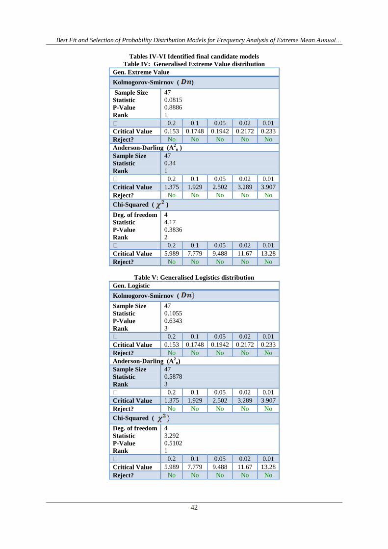
Best Fit and Selection of Probability Distribution Models for Frequency Analysis of Extreme Mean Annualhellip
42
Tables IV-VI Identified final candidate models
Table IV Generalised Extreme Value distribution
Gen Extreme Value
Kolmogorov-Smirnov ( )
Sample Size
Statistic
P-Value
Rank
47
00815
08886
1
02 01 005 002 001
Critical Value 0153 01748 01942 02172 0233
Reject No No No No No
Anderson-Darling (A2
n )
Sample Size
Statistic
Rank
47
034
1
02 01 005 002 001
Critical Value 1375 1929 2502 3289 3907
Reject No No No No No
Chi-Squared ( )
Deg of freedom
Statistic
P-Value
Rank
4
417
03836
2
02 01 005 002 001
Critical Value 5989 7779 9488 1167 1328
Reject No No No No No
Table V Generalised Logistics distribution
Gen Logistic
Kolmogorov-Smirnov (
Sample Size
Statistic
P-Value
Rank
47
01055
06343
3
02 01 005 002 001
Critical Value 0153 01748 01942 02172 0233
Reject No No No No No
Anderson-Darling (A2
n)
Sample Size
Statistic
Rank
47
05878
3
02 01 005 002 001
Critical Value 1375 1929 2502 3289 3907
Reject No No No No No
Chi-Squared (
Deg of freedom
Statistic
P-Value
Rank
4
3292
05102
1
02 01 005 002 001
Critical Value 5989 7779 9488 1167 1328
Reject No No No No No
Best Fit and Selection of Probability Distribution Models for Frequency Analysis of Extreme Mean Annualhellip
43
Table VI Log-Pearson distribution
Log-Pearson 3
Kolmogorov-Smirnov ( )
Sample Size
Statistic
P-Value
Rank
47
00899
08093
2
02 01 005 002 001
Critical Value 0153 01748 01942 02172 0233
Reject No No No No No
Anderson-Darling ( A2n)
Sample Size
Statistic
Rank
47
03954
2
02 01 005 002 001
Critical Value 1375 1929 2502 3289 3907
Reject No No No No No
Chi-Squared (
Deg of freedom
Statistic
P-Value
Rank
5
433
05029
3
02 01 005 002 001
Critical Value 7289 9236 1107 1339 1509
Reject No No No No No
Table VII Candidate models for modeling the distribution of extreme low mean annual rainfall events in 8
rainfall zones in Sabie river catchment
Distribution CDF or PDF Domain
Generalized Extreme
Value
Generalized Logistics
Log-Pearson 3
D Results of identification of best-fit models for frequency analysis of extreme low mean annual rainfall
events in Sabie river catchment
The best fit models for frequency analysis of extreme low mean annual rainfall events in 8 rainfall
zones in Sabie river catchment are presented in tables VII-XV The summary of the results of the best fit model
identification is presented in table XVI
Table VIII Best fit model Zone X3 a1
Distribution Kolmogorov
Smirnov
Anderson
Darling
A2
n
Chi-Squared
Abs(1- LSSMIC Best fit
Statistic Statistic Statistic
Gen Extreme Value 0079 0234 2898 1898 2211
Gen Logistic 0102 0531 2863 1863 2496
Log-Pearson 3 0093 0381 1270 0270 0744 X
Best Fit and Selection of Probability Distribution Models for Frequency Analysis of Extreme Mean Annualhellip
44
Table IX Best fit model Zone X3a2
Distribution Kolmogorov
Smirnov
Anderson
Darling
A2n
Chi-Squared (
Abs (1- LSSMIC Best fit
Statistic Statistic Statistic
Gen Logistic 0105 0587 3292 2292 2984 x
Gen Extreme Value 0081 0340 4170 3170 3591
Log-Pearson 3 0089 0395 4330 3330 3814
Table X Best fit model Zone X3b
Distribution Kolmogorov
Smirnov
Anderson
Darling A2n
Chi-Squared ( Abs (1- LSSMIC Best fit
Statistic Statistic Statistic
Gen Logistic 0073 0302 2653 1653 2028 x
Johnson SB 0089 0241 5127 4127 4457
Log-Pearson 3 0077 0273 7055 6055 6405
Table XI Best fit model Zone X31c
Distribution Kolmogorov
Smirnov
Anderson
Darling(
A2n)
Chi-
Squared
(
Abs (1-
LSSMIC Best
fit
Statistic Statistic Statistic
Gen Extreme Value 0042 0133 0350 0649 0824
Log-Pearson 3 0059 0248 0866 0133 0440 x
Gen Logistic 0069 0286 2065 1065 1420
Table XII Best fit model Zone X3d1
Distribution Kolmogorov
Smirnov (
Anderson
Darling
(A2
n)
Chi-Squared
(
Abs ( 1- LSSMIC Best fit
Statistic Statistic Statistic
Wakeby 0088 1362 3262 2262 3712
Gen Logistic 0106 0516 3950 2950 3572 x
Gen Extreme Value 0097 0446 5923 4923 5466
Table XII Best fit model Zone X3d2
Distribution Kolmogorov
Smirnov
Anderson
Darling
(A2n)
Chi-Squared
(
Abs (1- LSSMIC Best fit
Statistic Statistic Statistic
Gen Extreme Value 0054 0118 0799 0201 0373 x
Gen Logistic 0082 0191 1334 0334 0607
Log-Pearson 3 0055 0124 1553 0553 0732
Table XIV Best fit model Zone X3e
Distribution Kolmogorov
Smirnov
Anderson
Darling
A2
n
Chi-Squared
(
Abs(1- LSSMIC Best fit
Statistic Statistic Statistic
Gen Extreme Value 0088 0461 2029 1029 1578 X
Gen Logistic 0107 0771 3415 2415 3293
Log-Pearson 3 0125 0770 3432 2432 3327
Best Fit and Selection of Probability Distribution Models for Frequency Analysis of Extreme Mean Annualhellip
45
Table XV Best fit model Zone X3f
Distribution Kolmogorov
Smirnov
Anderson
Darling (
A2n)
Chi-
Squared
(
Abs ( 1-
LSSMIC Best
fit
Statistic Statistic Statistic
Log-Pearson 3 0072 0401 1244 0244 0717 X
Gen Extreme Value 0057 0265 1843 0843 1165
Gen Logistic 0092 0560 4527 3527 4179
Table XVI Summary of best fit model identification results
Best fit model
Log-Pearson 3
Rainfall zones
3 375
Generalized Logistic 3 375
Generalized Extreme Value 2 25
Totals 8 100
Log- Pearson 3 and Generalised Logistic models each was the best fit models for frequency analysis of
extreme low mean annual rainfall events in 3 rainfall zones Generalised extreme value model was the best fit in
2 rainfall zones The results shows that there no single model which is the best fit for frequency analysis of all
low mean annual rainfall events in Sabie river catchment
Table XVII Best fit and QT-T models for frequency analysis of extreme low mean annual rainfall events
Rainfall
zone
Best fit
model
QT-T model
X3a1 LP 3
X3a2 GL
X3b GL
X3c LP 3
X3d1 GL
X3d2 GEV
X3e GEV
X3f LP 3
E Results of frequency analysis of extreme low mean annual rainfall events in 8 rainfall zones in water
deficit catchments in South Africa
The results of frequency analysis of extreme low mean annual rainfall events in the 8 zones of water
deficit catchments in South Africa are presented in table XVIII
Best Fit and Selection of Probability Distribution Models for Frequency Analysis of Extreme Mean Annualhellip
46
Table XVIII Recurrence intervals in years of extreme low mean annual rainfall events
F How CMIC and LSSMIC address common limitations of model identification criteria
General Information Criteria (GIC) can be expressed as
31
where is the measure lack of fit by model
is the dimension of defined as the number of free parameter under model
is the penalty for complexity of the model (Parsimony)
may depend on effective sample size and dimension of (free parameters)
Addressing of limitations cited by Jiang (2014) by developing CMIC and LSSMIC was based on Equation 31
Emanating from this work and based on the results obtained thereof following can be considered with respect to
the previous cited limitations with the current model selection criteria
Limitation of effective sample size
In the case where the sample size is not equal to sample points this limitation is addressed by identifying
candidate models and best models based on characteristic of sample probability tail events and hypothesis
significance levels Sample distribution tail shape and not size is applied In so doing the effect of sample size is
eliminated Kolomogrov-Smirnov goodness-of-fit index is a component of LSSMIC This index is generally not
influenced by the possible inequality of sample size against the sample points especially in case of correlations
Limitation due to dimension of the model (parameters)
For practical purposes as illustrated in previous sections the Anderson-Darling goodness-of-fit index has been
adjusted to address the complexity of the problem (Refer to Equation 211) Chi-Squared goodness-of-fit was
also adjusted to absolute index to address the limitation of dimension of the model (Refer to Equation 212(a))
Over and under parameter fitting limitation was also addressed in developing of absolute Chi-Squared index
(Refer to Equation 212(b) In this procedure parsimony was also addressed Both Anderson-Darling and Chi-
Squared indices are elements in LSSMIC
Limitation of ambiguity
Determination of LSSMIC index results into specific numbers which in turn reduces ambiguity A special case
is when parameters shape or scale of Wakeby model is equal to zero In that case Wakeby and Generalized
Pareto statistics are equal and if are the least then the two models are taken as the best fit
Rainfall
zone
Best-
fit
Mathematical model
Recurrence interval in years
5 10 25 50 100 200
X3a1 LP3
7706 7318 6984 6776 6624 647 6
X3a2 GL
9912 9855 9790 9749 9708 9671
X3b GL
9362 9030 8691 8484 8306 8152
X3c LP3 7167 6823 6678 6415 6290 6154
X3d1 GL
9260 8891 8459 8200 7973 7772
X3d2 GEV
8751 8417 8160 8044 7968 7899
X3e GEV
8627 8317 8093 7999 7940 7903
X3f LP3
7120 6801 6307 6045 5912 5782
Best Fit and Selection of Probability Distribution Models for Frequency Analysis of Extreme Mean Annualhellip
47
Limitation of Criterion of Optimality
CMIC and LSSMIC have been developed in such a way that other parameters can be included This approach
ensures that technical and social parameters or variables can be included when needed In this particular case
peaks under threshold models have been included This could practically be assigned to the demand for water
resources needed at catchment level
Limitation of small sample and extreme events
This limitation is deemed to be solved by including Anderson-Darling and Kolomogrov-Smirnov in LSSMIC as
both cater for small sample and extreme events scenarios
IV CONCLUSION The main objective of this study was to develop two model identification criteria for frequency
analysis of extreme low mean rainfall events in water deficit catchments in South Africa The two model
selection criteria which were developed are
1 Candidate Model Identification Criterion (CM1C) for identifying candidate models
2 Least Sum of Statistics Model Identification Criterion ( LSSM1C) for identifying the best fit models for
frequency analysis of the extreme low mean annual rainfall events from the identified candidate models
The two developed criteria were applied to identify candidate models and best fit models for frequency analyses
of the extreme low mean annual rainfall events in 8 rainfall zones in Sabie river catchment Results obtained
showed that there no single probability distribution function is the best fit for all the 8 rainfall zones (table XVI)
Log-Pearson 3 (LP3) probability distribution function has been recommended for design hydro-
meteorological events mostly flood and drought in South Africa (Alexander 1990 2001) From the results of
this study Log-Pearson 3 may not be the only best fit model for frequency analyses of extreme hydro-
meteorological events in South Africa It is therefore important to carry out model identification processes to
identify best fit model for the specific required frequency analysis
Probability-Probability (P-P) plots were applied to evaluate the performance of CMIC and LSSMISC
The plots showed that CMIC and LSSMIC performed fairly well Although the Probability-Probability (P-P)
plot results cannot be considered completely conclusive CMIC and LSSMSC criteria make useful tools as
model selection method for frequency analysis of extreme mean annual rainfall events
ACKNOWLEDGEMENT The study has been supported by the Provincial Dept of Agriculture Rural Development Land and
Environmental Affairs Mpumalanga Provincial Government South Africa
REFERENCES [1] Akaike H 1974`` A new look at the statistical model identificationrsquorsquoIEEE Transaction on automatic
control vol 6 pp 716-725
[2] Alexander WJR 1990 Flood Hydrology for Southern Africa SANCOLD Pretoria RSA
[3] Alexander WJR 2001 Flood Risk Reduction Measures University of Pretoria Pretoria RSA
[4] Alexander WJR 2002a The standard design flood Journal of the South Africa Institution of Civil
[5] Engineers 44 (1)26-31
[6] Anderson TW Darling DA 1952 Asymptotic theory of certain goodness-of-fit criteria based on
[7] stochastic processes AnnMatStat 23 193-212
[8] AndersonD R and Burnham K P 2002 Avoiding pitfalls when using information-theoretic
methods Journal of wildlife management 66(3) 912-918
[9] Beven K J 2000 Rain-Run-off modeling The Primer John Wiley and sons Chichester UK 360
360pp
[10] Bobee B and Rasmussen P F 1995 Recent advances in flood frequency analysis Reviews of
Geophysics supplement July 1111-1116
[11] Bodini A and Cossu Q A 2010 Vulnerability assessment of Central-East Sardinia ( Italy) to
extreme rainfall events Journal of Natural hazards and Earth systems sciences 10 Pp 61-77
[12] Claeskens G Hjort NL 2003 The focused Information Criterion Journal of the American statistical
[13] Association 98 900-916
[14] FeyenHMJ 1970 Identification of run-off processes in catchments with a small scale topograph
[15] Furrer E M and Katz R W 2008 ``Improving the simulation of extreme precipitation events by
stochastic weather generatorsrsquorsquo Water Resources Research 44 W 12439doi 10292008 WR 007316
2008
[16] Gericke OJ 2010 Evaluation of the SDF method using a customized Design Flood Estimation Tool
University of Stellenbosch Stellenbosch South Africa 480 pp
Best Fit and Selection of Probability Distribution Models for Frequency Analysis of Extreme Mean Annualhellip
48
[17] Gorgens A H M Joint Peak- Volume ( JPV) Design Flood Hydrographs for South Africa WRC
Report 1420307 Water Research Commission Pretoria South Africa
[18] Gorgens A H M LysonsS Hayes L Makhabana M and Maluleke D 2007 Modernised South
African Design Floo Pro actce in the context of Dam safety WRC Report 1420 2 07 Water
Research omission Pretoria South Africa
[19] Goswani P and Ramesh K V 2007 Extreme rainfall events Vulnerability Analysis for Disaster
Management and Observation Systems Design Research Report CSIR PP21
[20] Hernandez A R P Balling R C Jr and Barber-Matinez 2009 Comparative analysis of indices of
extreme rainfall events Variation and trend from Southern Mexico Journal de Atmosfera 2 pages 219-
228
[21] Hosking JRM 1990 L-moments Analysis and estimation of distribution using Linear combinations
of
[22] order statistics Journal of the Royal statistics society Series B 52 105-124
[23] Hosking JRM Wallis JR Wood EF 1985 Estimation of the generalized extreme-value
distribution
[24] by the method of probability-weighted moments Technimetrics 27 (3) pp 251-261
[25] Hjort NL Claeskens G 2003 Rejoinder to the focused
[26] Jiang J 2014 The fence method Advances in statistics Volume 2014 Article ID 38081
[27] Kidson R Richards KS Carling PA 2005 Reconstructing the Ca-100 year flood in Northern
[28] Thailand Geomorphology 70 (2-4) 279-595
[29] Kottegoda NT Rosso R 1998 Statistics Probability and Reliability for Civil and Environmental
[30] Engineers McGrawHill New York
[31] Laio etal 2009 Model selection techniques for the frequency analysis of hydrological extremes
water
[32] Research Vol45 W07416
[33] Laio F 2004 Cramer-Von Mises and Anderson-Darling goodness-of-fit tests for extreme value
[34] distributions with unknown parameters Water Resources Research 40 W09308
[35] doi1010292004WR003204
[36] Mathwave(2011) httpwwwmathwavecom
[37] Mallows CL 1995 Some comments on Cp Technimetrics 37 362-372
[38] Mallows CL 1973 Some comments on Cp Technimetrics 15 661-675
[39] Meiz R and Bloschl G 2004 Regionaliisation of catchment model parameters J Hydrol 287 pp 95-
123
[40] Mkhandi SH Kachroo RK Gunasekara TAG 2000 Flood frequency analysis of Southern
Africa
[41] II Identification of regional distributions Hydrological Sciences Journal 45(3)449-464
[42] Mutua FM 1994 The use of the Akaike Information Criterion in the identification of an optimum
flood
[43] frequency model Hydro SciJ39 (3) 235-244
[44] Salami A W ( 2004) Prediction of the annual flow regime along Asa River using probability
distribution models AMSE periodicals Lyon France Modeling c-2004 65 (2) 41-56 ( httpamse-
modelingorgcontentamse 2004 htm)
[45] Schwarz G 1978 Estimating the dimension of a model Annals stat 6 461-464
[46] Schulze RE 1989 Non-stationary catchment responses and other problems in determing flood
series A case for a simulation modeling approach In Kienzle S W Maaren H (Eds) Proceedings
of the Fourth South African National Hyrological Symposium SANCIAHS Pretoria RSA pp 135-157
[47] ShamirE 2005 2004Application of temporal streamflow descriptors in hydrologic model parameter
estimationWater Resource Research 41 doi 10 10292004 WR 003409 SSN 0043-1397
[48] Shao J Sitter RR 1996 Bootstrip for imprinted Survey data Journal of the American statistical
[49] Association 93 819-831
[50] Smithers JC Schulze RE 2001 Design runoff estimation A review with reference to practices in
[51] South Africa Proceedings of Tenth South Africa National Hydrology Symposium 26-28 September
[52] 2001 School of BEEH University of Natal Pietermaritzburg RSA
[53] Smithers JC Schulze RE 2003 Design rainfall and flood estimation in South AfricaWRC Report
No
[54] 10600103 Water Research Commission Pretoria RSA
[55] Stedinger JR Vogel RM Foufoula E 1993 Frequency analysis of extreme events in Handbook
of
[56] Hydrology DR McGrawHill chap 18 66pp
Best Fit and Selection of Probability Distribution Models for Frequency Analysis of Extreme Mean Annualhellip
49
[57] Stedinger JR 1980 Fitting log normal distribution to hydrologic data Water Resource research
16(3)
[58] pp 481-490
[59] Stephens MA 1976 Asymptotic results for goodness-of-fit statistics with unknown parameters Ann
[60] Stat Vol 4 357-369
[61] Van der Linde A 2005 DIC in variable selection statistical Neerlandica 59 45-56
[62] Van der Linde A 2004 DIC in variable selection Technical report Institute of statistics University of
[63] Bremen httpwwwmathuni-bremende$simsard1downloadpapersvarse12pdf
[64] Wellner JA 1977 Aglirenko-Cantelli Theorem and strong laws of large numbers for function of
order
[65] statistics The annual of statistics vol5 number 3 1977 473-480
[66] Wilks DS 1998 Multi-site generalization of daily stochastic precipitation model J Hydro 210 178-
191
[67] Willens P Olsson J Ambjerg_Nielsen BeechamS Pathirana A BulowGregersen MadsenH and
Nguyen VTV 2007 Impact of climate change on rainfall extreme and urban drainage systems pp19-
20
[68] WMO- World Meteorological organization 1988 Analysing long Time Series of Hydrological data
with respect of climat variability WCAP-No 3 WMO-TD No 224
[69] WMO- World Meteorological organization 2009 Guidelines on Analysis of extremes in a changing
climate in support of informed decisions for adaptations WCDMP-No 72 WMO-TD No 1500
[70] Yua-Ping Xu Booij Martin J Tong Yang_Bin 2010 Uncertainity analysis in statistical modeling of
extreme hydrological events
[71] Yue S and Wang 2004 The Mann-Kendall test modified by effective sample size to detect trend in
serially correlated hydrological series Journal of Water Resources Management 18 Pages 201-218
Appendix A Probability-Probability (P-P) plots for extreme low mean rainfall events for the
8 rainfall zones
P-P Plot Zone X3a1
Gen Extreme Value Gen Logistic Log-Pearson 3
P (Empirical)
1090807060504030201
P (
Mo
de
l)
1
09
08
07
06
05
04
03
02
01
0
Fig 1 P-P plot Zone x3a1 Extreme mean annual rainfall events
Best Fit and Selection of Probability Distribution Models for Frequency Analysis of Extreme Mean Annualhellip
50
P-P Plot Zone x3a2
Gen Extreme Value Gen Logistic Log-Pearson 3
P (Empirical)
1090807060504030201
P (
Mo
de
l)
1
09
08
07
06
05
04
03
02
01
0
Fig 2 P-P plot Zone x3a2 Extreme mean annual rainfall events
P-P Plot Zone x3b
Gen Logistic Log-Pearson 3 Wakeby
P (Empirical)
1090807060504030201
P (
Model)
1
09
08
07
06
05
04
03
02
01
0
Fig 3 P-P plot Zone x3b Extreme mean annual rainfall events
Best Fit and Selection of Probability Distribution Models for Frequency Analysis of Extreme Mean Annualhellip
51
P-P Plot Zone x3c
Gen Extreme Value Gen Logistic Log-Pearson 3
P (Empirical)
10908070605040302010
P (
Model)
1
09
08
07
06
05
04
03
02
01
0
Fig4 P-P plot Zone x3c Extreme mean annual rainfall events
P-P Plot Zone x3d1
Gen Extreme Value Gen Logistic Wakeby
P (Empirical)
10908070605040302010
P (
Model)
1
09
08
07
06
05
04
03
02
01
0
Fig 5 P-P plot Zone x3d1 Extreme mean annual rainfall events
Best Fit and Selection of Probability Distribution Models for Frequency Analysis of Extreme Mean Annualhellip
52
P-P Plot Zone x3d2
Gen Extreme Value Gen Logistic Log-Pearson 3
P (Empirical)
1090807060504030201
P (
Model)
1
09
08
07
06
05
04
03
02
01
0
FIG 6 P-P plot Zone x3d2 Extreme mean annual rainfall events
P-P Plot Zone x3e
Gen Extreme Value Gen Logistic Log-Pearson 3
P (Empirical)
1080604020
P (
Model)
1
09
08
07
06
05
04
03
02
01
0
Fig 7 P-P plot Zone x3e Extreme mean annual rainfall events
Best Fit and Selection of Probability Distribution Models for Frequency Analysis of Extreme Mean Annualhellip
53
P-P Plot Zone x3f
Gen Extreme Value Gen Logistic Log-Pearson 3
P (Empirical)
1090807060504030201
P (
Mo
de
l)
1
09
08
07
06
05
04
03
02
01
0
Fig8 P-P plot Zone x3f Extreme mean annual rainfall events
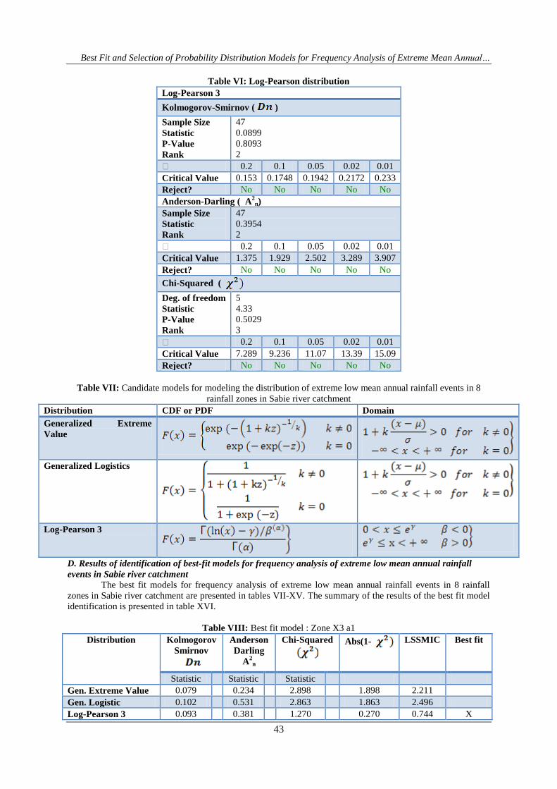
Best Fit and Selection of Probability Distribution Models for Frequency Analysis of Extreme Mean Annualhellip
43
Table VI Log-Pearson distribution
Log-Pearson 3
Kolmogorov-Smirnov ( )
Sample Size
Statistic
P-Value
Rank
47
00899
08093
2
02 01 005 002 001
Critical Value 0153 01748 01942 02172 0233
Reject No No No No No
Anderson-Darling ( A2n)
Sample Size
Statistic
Rank
47
03954
2
02 01 005 002 001
Critical Value 1375 1929 2502 3289 3907
Reject No No No No No
Chi-Squared (
Deg of freedom
Statistic
P-Value
Rank
5
433
05029
3
02 01 005 002 001
Critical Value 7289 9236 1107 1339 1509
Reject No No No No No
Table VII Candidate models for modeling the distribution of extreme low mean annual rainfall events in 8
rainfall zones in Sabie river catchment
Distribution CDF or PDF Domain
Generalized Extreme
Value
Generalized Logistics
Log-Pearson 3
D Results of identification of best-fit models for frequency analysis of extreme low mean annual rainfall
events in Sabie river catchment
The best fit models for frequency analysis of extreme low mean annual rainfall events in 8 rainfall
zones in Sabie river catchment are presented in tables VII-XV The summary of the results of the best fit model
identification is presented in table XVI
Table VIII Best fit model Zone X3 a1
Distribution Kolmogorov
Smirnov
Anderson
Darling
A2
n
Chi-Squared
Abs(1- LSSMIC Best fit
Statistic Statistic Statistic
Gen Extreme Value 0079 0234 2898 1898 2211
Gen Logistic 0102 0531 2863 1863 2496
Log-Pearson 3 0093 0381 1270 0270 0744 X
Best Fit and Selection of Probability Distribution Models for Frequency Analysis of Extreme Mean Annualhellip
44
Table IX Best fit model Zone X3a2
Distribution Kolmogorov
Smirnov
Anderson
Darling
A2n
Chi-Squared (
Abs (1- LSSMIC Best fit
Statistic Statistic Statistic
Gen Logistic 0105 0587 3292 2292 2984 x
Gen Extreme Value 0081 0340 4170 3170 3591
Log-Pearson 3 0089 0395 4330 3330 3814
Table X Best fit model Zone X3b
Distribution Kolmogorov
Smirnov
Anderson
Darling A2n
Chi-Squared ( Abs (1- LSSMIC Best fit
Statistic Statistic Statistic
Gen Logistic 0073 0302 2653 1653 2028 x
Johnson SB 0089 0241 5127 4127 4457
Log-Pearson 3 0077 0273 7055 6055 6405
Table XI Best fit model Zone X31c
Distribution Kolmogorov
Smirnov
Anderson
Darling(
A2n)
Chi-
Squared
(
Abs (1-
LSSMIC Best
fit
Statistic Statistic Statistic
Gen Extreme Value 0042 0133 0350 0649 0824
Log-Pearson 3 0059 0248 0866 0133 0440 x
Gen Logistic 0069 0286 2065 1065 1420
Table XII Best fit model Zone X3d1
Distribution Kolmogorov
Smirnov (
Anderson
Darling
(A2
n)
Chi-Squared
(
Abs ( 1- LSSMIC Best fit
Statistic Statistic Statistic
Wakeby 0088 1362 3262 2262 3712
Gen Logistic 0106 0516 3950 2950 3572 x
Gen Extreme Value 0097 0446 5923 4923 5466
Table XII Best fit model Zone X3d2
Distribution Kolmogorov
Smirnov
Anderson
Darling
(A2n)
Chi-Squared
(
Abs (1- LSSMIC Best fit
Statistic Statistic Statistic
Gen Extreme Value 0054 0118 0799 0201 0373 x
Gen Logistic 0082 0191 1334 0334 0607
Log-Pearson 3 0055 0124 1553 0553 0732
Table XIV Best fit model Zone X3e
Distribution Kolmogorov
Smirnov
Anderson
Darling
A2
n
Chi-Squared
(
Abs(1- LSSMIC Best fit
Statistic Statistic Statistic
Gen Extreme Value 0088 0461 2029 1029 1578 X
Gen Logistic 0107 0771 3415 2415 3293
Log-Pearson 3 0125 0770 3432 2432 3327
Best Fit and Selection of Probability Distribution Models for Frequency Analysis of Extreme Mean Annualhellip
45
Table XV Best fit model Zone X3f
Distribution Kolmogorov
Smirnov
Anderson
Darling (
A2n)
Chi-
Squared
(
Abs ( 1-
LSSMIC Best
fit
Statistic Statistic Statistic
Log-Pearson 3 0072 0401 1244 0244 0717 X
Gen Extreme Value 0057 0265 1843 0843 1165
Gen Logistic 0092 0560 4527 3527 4179
Table XVI Summary of best fit model identification results
Best fit model
Log-Pearson 3
Rainfall zones
3 375
Generalized Logistic 3 375
Generalized Extreme Value 2 25
Totals 8 100
Log- Pearson 3 and Generalised Logistic models each was the best fit models for frequency analysis of
extreme low mean annual rainfall events in 3 rainfall zones Generalised extreme value model was the best fit in
2 rainfall zones The results shows that there no single model which is the best fit for frequency analysis of all
low mean annual rainfall events in Sabie river catchment
Table XVII Best fit and QT-T models for frequency analysis of extreme low mean annual rainfall events
Rainfall
zone
Best fit
model
QT-T model
X3a1 LP 3
X3a2 GL
X3b GL
X3c LP 3
X3d1 GL
X3d2 GEV
X3e GEV
X3f LP 3
E Results of frequency analysis of extreme low mean annual rainfall events in 8 rainfall zones in water
deficit catchments in South Africa
The results of frequency analysis of extreme low mean annual rainfall events in the 8 zones of water
deficit catchments in South Africa are presented in table XVIII
Best Fit and Selection of Probability Distribution Models for Frequency Analysis of Extreme Mean Annualhellip
46
Table XVIII Recurrence intervals in years of extreme low mean annual rainfall events
F How CMIC and LSSMIC address common limitations of model identification criteria
General Information Criteria (GIC) can be expressed as
31
where is the measure lack of fit by model
is the dimension of defined as the number of free parameter under model
is the penalty for complexity of the model (Parsimony)
may depend on effective sample size and dimension of (free parameters)
Addressing of limitations cited by Jiang (2014) by developing CMIC and LSSMIC was based on Equation 31
Emanating from this work and based on the results obtained thereof following can be considered with respect to
the previous cited limitations with the current model selection criteria
Limitation of effective sample size
In the case where the sample size is not equal to sample points this limitation is addressed by identifying
candidate models and best models based on characteristic of sample probability tail events and hypothesis
significance levels Sample distribution tail shape and not size is applied In so doing the effect of sample size is
eliminated Kolomogrov-Smirnov goodness-of-fit index is a component of LSSMIC This index is generally not
influenced by the possible inequality of sample size against the sample points especially in case of correlations
Limitation due to dimension of the model (parameters)
For practical purposes as illustrated in previous sections the Anderson-Darling goodness-of-fit index has been
adjusted to address the complexity of the problem (Refer to Equation 211) Chi-Squared goodness-of-fit was
also adjusted to absolute index to address the limitation of dimension of the model (Refer to Equation 212(a))
Over and under parameter fitting limitation was also addressed in developing of absolute Chi-Squared index
(Refer to Equation 212(b) In this procedure parsimony was also addressed Both Anderson-Darling and Chi-
Squared indices are elements in LSSMIC
Limitation of ambiguity
Determination of LSSMIC index results into specific numbers which in turn reduces ambiguity A special case
is when parameters shape or scale of Wakeby model is equal to zero In that case Wakeby and Generalized
Pareto statistics are equal and if are the least then the two models are taken as the best fit
Rainfall
zone
Best-
fit
Mathematical model
Recurrence interval in years
5 10 25 50 100 200
X3a1 LP3
7706 7318 6984 6776 6624 647 6
X3a2 GL
9912 9855 9790 9749 9708 9671
X3b GL
9362 9030 8691 8484 8306 8152
X3c LP3 7167 6823 6678 6415 6290 6154
X3d1 GL
9260 8891 8459 8200 7973 7772
X3d2 GEV
8751 8417 8160 8044 7968 7899
X3e GEV
8627 8317 8093 7999 7940 7903
X3f LP3
7120 6801 6307 6045 5912 5782
Best Fit and Selection of Probability Distribution Models for Frequency Analysis of Extreme Mean Annualhellip
47
Limitation of Criterion of Optimality
CMIC and LSSMIC have been developed in such a way that other parameters can be included This approach
ensures that technical and social parameters or variables can be included when needed In this particular case
peaks under threshold models have been included This could practically be assigned to the demand for water
resources needed at catchment level
Limitation of small sample and extreme events
This limitation is deemed to be solved by including Anderson-Darling and Kolomogrov-Smirnov in LSSMIC as
both cater for small sample and extreme events scenarios
IV CONCLUSION The main objective of this study was to develop two model identification criteria for frequency
analysis of extreme low mean rainfall events in water deficit catchments in South Africa The two model
selection criteria which were developed are
1 Candidate Model Identification Criterion (CM1C) for identifying candidate models
2 Least Sum of Statistics Model Identification Criterion ( LSSM1C) for identifying the best fit models for
frequency analysis of the extreme low mean annual rainfall events from the identified candidate models
The two developed criteria were applied to identify candidate models and best fit models for frequency analyses
of the extreme low mean annual rainfall events in 8 rainfall zones in Sabie river catchment Results obtained
showed that there no single probability distribution function is the best fit for all the 8 rainfall zones (table XVI)
Log-Pearson 3 (LP3) probability distribution function has been recommended for design hydro-
meteorological events mostly flood and drought in South Africa (Alexander 1990 2001) From the results of
this study Log-Pearson 3 may not be the only best fit model for frequency analyses of extreme hydro-
meteorological events in South Africa It is therefore important to carry out model identification processes to
identify best fit model for the specific required frequency analysis
Probability-Probability (P-P) plots were applied to evaluate the performance of CMIC and LSSMISC
The plots showed that CMIC and LSSMIC performed fairly well Although the Probability-Probability (P-P)
plot results cannot be considered completely conclusive CMIC and LSSMSC criteria make useful tools as
model selection method for frequency analysis of extreme mean annual rainfall events
ACKNOWLEDGEMENT The study has been supported by the Provincial Dept of Agriculture Rural Development Land and
Environmental Affairs Mpumalanga Provincial Government South Africa
REFERENCES [1] Akaike H 1974`` A new look at the statistical model identificationrsquorsquoIEEE Transaction on automatic
control vol 6 pp 716-725
[2] Alexander WJR 1990 Flood Hydrology for Southern Africa SANCOLD Pretoria RSA
[3] Alexander WJR 2001 Flood Risk Reduction Measures University of Pretoria Pretoria RSA
[4] Alexander WJR 2002a The standard design flood Journal of the South Africa Institution of Civil
[5] Engineers 44 (1)26-31
[6] Anderson TW Darling DA 1952 Asymptotic theory of certain goodness-of-fit criteria based on
[7] stochastic processes AnnMatStat 23 193-212
[8] AndersonD R and Burnham K P 2002 Avoiding pitfalls when using information-theoretic
methods Journal of wildlife management 66(3) 912-918
[9] Beven K J 2000 Rain-Run-off modeling The Primer John Wiley and sons Chichester UK 360
360pp
[10] Bobee B and Rasmussen P F 1995 Recent advances in flood frequency analysis Reviews of
Geophysics supplement July 1111-1116
[11] Bodini A and Cossu Q A 2010 Vulnerability assessment of Central-East Sardinia ( Italy) to
extreme rainfall events Journal of Natural hazards and Earth systems sciences 10 Pp 61-77
[12] Claeskens G Hjort NL 2003 The focused Information Criterion Journal of the American statistical
[13] Association 98 900-916
[14] FeyenHMJ 1970 Identification of run-off processes in catchments with a small scale topograph
[15] Furrer E M and Katz R W 2008 ``Improving the simulation of extreme precipitation events by
stochastic weather generatorsrsquorsquo Water Resources Research 44 W 12439doi 10292008 WR 007316
2008
[16] Gericke OJ 2010 Evaluation of the SDF method using a customized Design Flood Estimation Tool
University of Stellenbosch Stellenbosch South Africa 480 pp
Best Fit and Selection of Probability Distribution Models for Frequency Analysis of Extreme Mean Annualhellip
48
[17] Gorgens A H M Joint Peak- Volume ( JPV) Design Flood Hydrographs for South Africa WRC
Report 1420307 Water Research Commission Pretoria South Africa
[18] Gorgens A H M LysonsS Hayes L Makhabana M and Maluleke D 2007 Modernised South
African Design Floo Pro actce in the context of Dam safety WRC Report 1420 2 07 Water
Research omission Pretoria South Africa
[19] Goswani P and Ramesh K V 2007 Extreme rainfall events Vulnerability Analysis for Disaster
Management and Observation Systems Design Research Report CSIR PP21
[20] Hernandez A R P Balling R C Jr and Barber-Matinez 2009 Comparative analysis of indices of
extreme rainfall events Variation and trend from Southern Mexico Journal de Atmosfera 2 pages 219-
228
[21] Hosking JRM 1990 L-moments Analysis and estimation of distribution using Linear combinations
of
[22] order statistics Journal of the Royal statistics society Series B 52 105-124
[23] Hosking JRM Wallis JR Wood EF 1985 Estimation of the generalized extreme-value
distribution
[24] by the method of probability-weighted moments Technimetrics 27 (3) pp 251-261
[25] Hjort NL Claeskens G 2003 Rejoinder to the focused
[26] Jiang J 2014 The fence method Advances in statistics Volume 2014 Article ID 38081
[27] Kidson R Richards KS Carling PA 2005 Reconstructing the Ca-100 year flood in Northern
[28] Thailand Geomorphology 70 (2-4) 279-595
[29] Kottegoda NT Rosso R 1998 Statistics Probability and Reliability for Civil and Environmental
[30] Engineers McGrawHill New York
[31] Laio etal 2009 Model selection techniques for the frequency analysis of hydrological extremes
water
[32] Research Vol45 W07416
[33] Laio F 2004 Cramer-Von Mises and Anderson-Darling goodness-of-fit tests for extreme value
[34] distributions with unknown parameters Water Resources Research 40 W09308
[35] doi1010292004WR003204
[36] Mathwave(2011) httpwwwmathwavecom
[37] Mallows CL 1995 Some comments on Cp Technimetrics 37 362-372
[38] Mallows CL 1973 Some comments on Cp Technimetrics 15 661-675
[39] Meiz R and Bloschl G 2004 Regionaliisation of catchment model parameters J Hydrol 287 pp 95-
123
[40] Mkhandi SH Kachroo RK Gunasekara TAG 2000 Flood frequency analysis of Southern
Africa
[41] II Identification of regional distributions Hydrological Sciences Journal 45(3)449-464
[42] Mutua FM 1994 The use of the Akaike Information Criterion in the identification of an optimum
flood
[43] frequency model Hydro SciJ39 (3) 235-244
[44] Salami A W ( 2004) Prediction of the annual flow regime along Asa River using probability
distribution models AMSE periodicals Lyon France Modeling c-2004 65 (2) 41-56 ( httpamse-
modelingorgcontentamse 2004 htm)
[45] Schwarz G 1978 Estimating the dimension of a model Annals stat 6 461-464
[46] Schulze RE 1989 Non-stationary catchment responses and other problems in determing flood
series A case for a simulation modeling approach In Kienzle S W Maaren H (Eds) Proceedings
of the Fourth South African National Hyrological Symposium SANCIAHS Pretoria RSA pp 135-157
[47] ShamirE 2005 2004Application of temporal streamflow descriptors in hydrologic model parameter
estimationWater Resource Research 41 doi 10 10292004 WR 003409 SSN 0043-1397
[48] Shao J Sitter RR 1996 Bootstrip for imprinted Survey data Journal of the American statistical
[49] Association 93 819-831
[50] Smithers JC Schulze RE 2001 Design runoff estimation A review with reference to practices in
[51] South Africa Proceedings of Tenth South Africa National Hydrology Symposium 26-28 September
[52] 2001 School of BEEH University of Natal Pietermaritzburg RSA
[53] Smithers JC Schulze RE 2003 Design rainfall and flood estimation in South AfricaWRC Report
No
[54] 10600103 Water Research Commission Pretoria RSA
[55] Stedinger JR Vogel RM Foufoula E 1993 Frequency analysis of extreme events in Handbook
of
[56] Hydrology DR McGrawHill chap 18 66pp
Best Fit and Selection of Probability Distribution Models for Frequency Analysis of Extreme Mean Annualhellip
49
[57] Stedinger JR 1980 Fitting log normal distribution to hydrologic data Water Resource research
16(3)
[58] pp 481-490
[59] Stephens MA 1976 Asymptotic results for goodness-of-fit statistics with unknown parameters Ann
[60] Stat Vol 4 357-369
[61] Van der Linde A 2005 DIC in variable selection statistical Neerlandica 59 45-56
[62] Van der Linde A 2004 DIC in variable selection Technical report Institute of statistics University of
[63] Bremen httpwwwmathuni-bremende$simsard1downloadpapersvarse12pdf
[64] Wellner JA 1977 Aglirenko-Cantelli Theorem and strong laws of large numbers for function of
order
[65] statistics The annual of statistics vol5 number 3 1977 473-480
[66] Wilks DS 1998 Multi-site generalization of daily stochastic precipitation model J Hydro 210 178-
191
[67] Willens P Olsson J Ambjerg_Nielsen BeechamS Pathirana A BulowGregersen MadsenH and
Nguyen VTV 2007 Impact of climate change on rainfall extreme and urban drainage systems pp19-
20
[68] WMO- World Meteorological organization 1988 Analysing long Time Series of Hydrological data
with respect of climat variability WCAP-No 3 WMO-TD No 224
[69] WMO- World Meteorological organization 2009 Guidelines on Analysis of extremes in a changing
climate in support of informed decisions for adaptations WCDMP-No 72 WMO-TD No 1500
[70] Yua-Ping Xu Booij Martin J Tong Yang_Bin 2010 Uncertainity analysis in statistical modeling of
extreme hydrological events
[71] Yue S and Wang 2004 The Mann-Kendall test modified by effective sample size to detect trend in
serially correlated hydrological series Journal of Water Resources Management 18 Pages 201-218
Appendix A Probability-Probability (P-P) plots for extreme low mean rainfall events for the
8 rainfall zones
P-P Plot Zone X3a1
Gen Extreme Value Gen Logistic Log-Pearson 3
P (Empirical)
1090807060504030201
P (
Mo
de
l)
1
09
08
07
06
05
04
03
02
01
0
Fig 1 P-P plot Zone x3a1 Extreme mean annual rainfall events
Best Fit and Selection of Probability Distribution Models for Frequency Analysis of Extreme Mean Annualhellip
50
P-P Plot Zone x3a2
Gen Extreme Value Gen Logistic Log-Pearson 3
P (Empirical)
1090807060504030201
P (
Mo
de
l)
1
09
08
07
06
05
04
03
02
01
0
Fig 2 P-P plot Zone x3a2 Extreme mean annual rainfall events
P-P Plot Zone x3b
Gen Logistic Log-Pearson 3 Wakeby
P (Empirical)
1090807060504030201
P (
Model)
1
09
08
07
06
05
04
03
02
01
0
Fig 3 P-P plot Zone x3b Extreme mean annual rainfall events
Best Fit and Selection of Probability Distribution Models for Frequency Analysis of Extreme Mean Annualhellip
51
P-P Plot Zone x3c
Gen Extreme Value Gen Logistic Log-Pearson 3
P (Empirical)
10908070605040302010
P (
Model)
1
09
08
07
06
05
04
03
02
01
0
Fig4 P-P plot Zone x3c Extreme mean annual rainfall events
P-P Plot Zone x3d1
Gen Extreme Value Gen Logistic Wakeby
P (Empirical)
10908070605040302010
P (
Model)
1
09
08
07
06
05
04
03
02
01
0
Fig 5 P-P plot Zone x3d1 Extreme mean annual rainfall events
Best Fit and Selection of Probability Distribution Models for Frequency Analysis of Extreme Mean Annualhellip
52
P-P Plot Zone x3d2
Gen Extreme Value Gen Logistic Log-Pearson 3
P (Empirical)
1090807060504030201
P (
Model)
1
09
08
07
06
05
04
03
02
01
0
FIG 6 P-P plot Zone x3d2 Extreme mean annual rainfall events
P-P Plot Zone x3e
Gen Extreme Value Gen Logistic Log-Pearson 3
P (Empirical)
1080604020
P (
Model)
1
09
08
07
06
05
04
03
02
01
0
Fig 7 P-P plot Zone x3e Extreme mean annual rainfall events
Best Fit and Selection of Probability Distribution Models for Frequency Analysis of Extreme Mean Annualhellip
53
P-P Plot Zone x3f
Gen Extreme Value Gen Logistic Log-Pearson 3
P (Empirical)
1090807060504030201
P (
Mo
de
l)
1
09
08
07
06
05
04
03
02
01
0
Fig8 P-P plot Zone x3f Extreme mean annual rainfall events
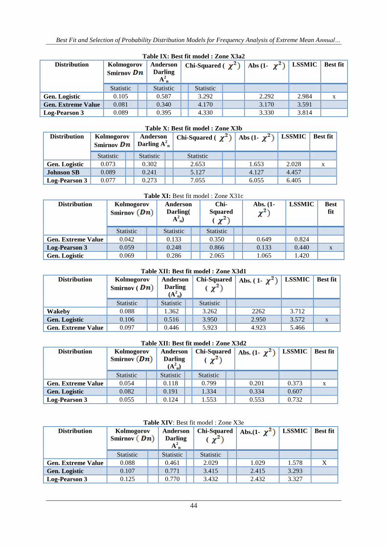
Best Fit and Selection of Probability Distribution Models for Frequency Analysis of Extreme Mean Annualhellip
44
Table IX Best fit model Zone X3a2
Distribution Kolmogorov
Smirnov
Anderson
Darling
A2n
Chi-Squared (
Abs (1- LSSMIC Best fit
Statistic Statistic Statistic
Gen Logistic 0105 0587 3292 2292 2984 x
Gen Extreme Value 0081 0340 4170 3170 3591
Log-Pearson 3 0089 0395 4330 3330 3814
Table X Best fit model Zone X3b
Distribution Kolmogorov
Smirnov
Anderson
Darling A2n
Chi-Squared ( Abs (1- LSSMIC Best fit
Statistic Statistic Statistic
Gen Logistic 0073 0302 2653 1653 2028 x
Johnson SB 0089 0241 5127 4127 4457
Log-Pearson 3 0077 0273 7055 6055 6405
Table XI Best fit model Zone X31c
Distribution Kolmogorov
Smirnov
Anderson
Darling(
A2n)
Chi-
Squared
(
Abs (1-
LSSMIC Best
fit
Statistic Statistic Statistic
Gen Extreme Value 0042 0133 0350 0649 0824
Log-Pearson 3 0059 0248 0866 0133 0440 x
Gen Logistic 0069 0286 2065 1065 1420
Table XII Best fit model Zone X3d1
Distribution Kolmogorov
Smirnov (
Anderson
Darling
(A2
n)
Chi-Squared
(
Abs ( 1- LSSMIC Best fit
Statistic Statistic Statistic
Wakeby 0088 1362 3262 2262 3712
Gen Logistic 0106 0516 3950 2950 3572 x
Gen Extreme Value 0097 0446 5923 4923 5466
Table XII Best fit model Zone X3d2
Distribution Kolmogorov
Smirnov
Anderson
Darling
(A2n)
Chi-Squared
(
Abs (1- LSSMIC Best fit
Statistic Statistic Statistic
Gen Extreme Value 0054 0118 0799 0201 0373 x
Gen Logistic 0082 0191 1334 0334 0607
Log-Pearson 3 0055 0124 1553 0553 0732
Table XIV Best fit model Zone X3e
Distribution Kolmogorov
Smirnov
Anderson
Darling
A2
n
Chi-Squared
(
Abs(1- LSSMIC Best fit
Statistic Statistic Statistic
Gen Extreme Value 0088 0461 2029 1029 1578 X
Gen Logistic 0107 0771 3415 2415 3293
Log-Pearson 3 0125 0770 3432 2432 3327
Best Fit and Selection of Probability Distribution Models for Frequency Analysis of Extreme Mean Annualhellip
45
Table XV Best fit model Zone X3f
Distribution Kolmogorov
Smirnov
Anderson
Darling (
A2n)
Chi-
Squared
(
Abs ( 1-
LSSMIC Best
fit
Statistic Statistic Statistic
Log-Pearson 3 0072 0401 1244 0244 0717 X
Gen Extreme Value 0057 0265 1843 0843 1165
Gen Logistic 0092 0560 4527 3527 4179
Table XVI Summary of best fit model identification results
Best fit model
Log-Pearson 3
Rainfall zones
3 375
Generalized Logistic 3 375
Generalized Extreme Value 2 25
Totals 8 100
Log- Pearson 3 and Generalised Logistic models each was the best fit models for frequency analysis of
extreme low mean annual rainfall events in 3 rainfall zones Generalised extreme value model was the best fit in
2 rainfall zones The results shows that there no single model which is the best fit for frequency analysis of all
low mean annual rainfall events in Sabie river catchment
Table XVII Best fit and QT-T models for frequency analysis of extreme low mean annual rainfall events
Rainfall
zone
Best fit
model
QT-T model
X3a1 LP 3
X3a2 GL
X3b GL
X3c LP 3
X3d1 GL
X3d2 GEV
X3e GEV
X3f LP 3
E Results of frequency analysis of extreme low mean annual rainfall events in 8 rainfall zones in water
deficit catchments in South Africa
The results of frequency analysis of extreme low mean annual rainfall events in the 8 zones of water
deficit catchments in South Africa are presented in table XVIII
Best Fit and Selection of Probability Distribution Models for Frequency Analysis of Extreme Mean Annualhellip
46
Table XVIII Recurrence intervals in years of extreme low mean annual rainfall events
F How CMIC and LSSMIC address common limitations of model identification criteria
General Information Criteria (GIC) can be expressed as
31
where is the measure lack of fit by model
is the dimension of defined as the number of free parameter under model
is the penalty for complexity of the model (Parsimony)
may depend on effective sample size and dimension of (free parameters)
Addressing of limitations cited by Jiang (2014) by developing CMIC and LSSMIC was based on Equation 31
Emanating from this work and based on the results obtained thereof following can be considered with respect to
the previous cited limitations with the current model selection criteria
Limitation of effective sample size
In the case where the sample size is not equal to sample points this limitation is addressed by identifying
candidate models and best models based on characteristic of sample probability tail events and hypothesis
significance levels Sample distribution tail shape and not size is applied In so doing the effect of sample size is
eliminated Kolomogrov-Smirnov goodness-of-fit index is a component of LSSMIC This index is generally not
influenced by the possible inequality of sample size against the sample points especially in case of correlations
Limitation due to dimension of the model (parameters)
For practical purposes as illustrated in previous sections the Anderson-Darling goodness-of-fit index has been
adjusted to address the complexity of the problem (Refer to Equation 211) Chi-Squared goodness-of-fit was
also adjusted to absolute index to address the limitation of dimension of the model (Refer to Equation 212(a))
Over and under parameter fitting limitation was also addressed in developing of absolute Chi-Squared index
(Refer to Equation 212(b) In this procedure parsimony was also addressed Both Anderson-Darling and Chi-
Squared indices are elements in LSSMIC
Limitation of ambiguity
Determination of LSSMIC index results into specific numbers which in turn reduces ambiguity A special case
is when parameters shape or scale of Wakeby model is equal to zero In that case Wakeby and Generalized
Pareto statistics are equal and if are the least then the two models are taken as the best fit
Rainfall
zone
Best-
fit
Mathematical model
Recurrence interval in years
5 10 25 50 100 200
X3a1 LP3
7706 7318 6984 6776 6624 647 6
X3a2 GL
9912 9855 9790 9749 9708 9671
X3b GL
9362 9030 8691 8484 8306 8152
X3c LP3 7167 6823 6678 6415 6290 6154
X3d1 GL
9260 8891 8459 8200 7973 7772
X3d2 GEV
8751 8417 8160 8044 7968 7899
X3e GEV
8627 8317 8093 7999 7940 7903
X3f LP3
7120 6801 6307 6045 5912 5782
Best Fit and Selection of Probability Distribution Models for Frequency Analysis of Extreme Mean Annualhellip
47
Limitation of Criterion of Optimality
CMIC and LSSMIC have been developed in such a way that other parameters can be included This approach
ensures that technical and social parameters or variables can be included when needed In this particular case
peaks under threshold models have been included This could practically be assigned to the demand for water
resources needed at catchment level
Limitation of small sample and extreme events
This limitation is deemed to be solved by including Anderson-Darling and Kolomogrov-Smirnov in LSSMIC as
both cater for small sample and extreme events scenarios
IV CONCLUSION The main objective of this study was to develop two model identification criteria for frequency
analysis of extreme low mean rainfall events in water deficit catchments in South Africa The two model
selection criteria which were developed are
1 Candidate Model Identification Criterion (CM1C) for identifying candidate models
2 Least Sum of Statistics Model Identification Criterion ( LSSM1C) for identifying the best fit models for
frequency analysis of the extreme low mean annual rainfall events from the identified candidate models
The two developed criteria were applied to identify candidate models and best fit models for frequency analyses
of the extreme low mean annual rainfall events in 8 rainfall zones in Sabie river catchment Results obtained
showed that there no single probability distribution function is the best fit for all the 8 rainfall zones (table XVI)
Log-Pearson 3 (LP3) probability distribution function has been recommended for design hydro-
meteorological events mostly flood and drought in South Africa (Alexander 1990 2001) From the results of
this study Log-Pearson 3 may not be the only best fit model for frequency analyses of extreme hydro-
meteorological events in South Africa It is therefore important to carry out model identification processes to
identify best fit model for the specific required frequency analysis
Probability-Probability (P-P) plots were applied to evaluate the performance of CMIC and LSSMISC
The plots showed that CMIC and LSSMIC performed fairly well Although the Probability-Probability (P-P)
plot results cannot be considered completely conclusive CMIC and LSSMSC criteria make useful tools as
model selection method for frequency analysis of extreme mean annual rainfall events
ACKNOWLEDGEMENT The study has been supported by the Provincial Dept of Agriculture Rural Development Land and
Environmental Affairs Mpumalanga Provincial Government South Africa
REFERENCES [1] Akaike H 1974`` A new look at the statistical model identificationrsquorsquoIEEE Transaction on automatic
control vol 6 pp 716-725
[2] Alexander WJR 1990 Flood Hydrology for Southern Africa SANCOLD Pretoria RSA
[3] Alexander WJR 2001 Flood Risk Reduction Measures University of Pretoria Pretoria RSA
[4] Alexander WJR 2002a The standard design flood Journal of the South Africa Institution of Civil
[5] Engineers 44 (1)26-31
[6] Anderson TW Darling DA 1952 Asymptotic theory of certain goodness-of-fit criteria based on
[7] stochastic processes AnnMatStat 23 193-212
[8] AndersonD R and Burnham K P 2002 Avoiding pitfalls when using information-theoretic
methods Journal of wildlife management 66(3) 912-918
[9] Beven K J 2000 Rain-Run-off modeling The Primer John Wiley and sons Chichester UK 360
360pp
[10] Bobee B and Rasmussen P F 1995 Recent advances in flood frequency analysis Reviews of
Geophysics supplement July 1111-1116
[11] Bodini A and Cossu Q A 2010 Vulnerability assessment of Central-East Sardinia ( Italy) to
extreme rainfall events Journal of Natural hazards and Earth systems sciences 10 Pp 61-77
[12] Claeskens G Hjort NL 2003 The focused Information Criterion Journal of the American statistical
[13] Association 98 900-916
[14] FeyenHMJ 1970 Identification of run-off processes in catchments with a small scale topograph
[15] Furrer E M and Katz R W 2008 ``Improving the simulation of extreme precipitation events by
stochastic weather generatorsrsquorsquo Water Resources Research 44 W 12439doi 10292008 WR 007316
2008
[16] Gericke OJ 2010 Evaluation of the SDF method using a customized Design Flood Estimation Tool
University of Stellenbosch Stellenbosch South Africa 480 pp
Best Fit and Selection of Probability Distribution Models for Frequency Analysis of Extreme Mean Annualhellip
48
[17] Gorgens A H M Joint Peak- Volume ( JPV) Design Flood Hydrographs for South Africa WRC
Report 1420307 Water Research Commission Pretoria South Africa
[18] Gorgens A H M LysonsS Hayes L Makhabana M and Maluleke D 2007 Modernised South
African Design Floo Pro actce in the context of Dam safety WRC Report 1420 2 07 Water
Research omission Pretoria South Africa
[19] Goswani P and Ramesh K V 2007 Extreme rainfall events Vulnerability Analysis for Disaster
Management and Observation Systems Design Research Report CSIR PP21
[20] Hernandez A R P Balling R C Jr and Barber-Matinez 2009 Comparative analysis of indices of
extreme rainfall events Variation and trend from Southern Mexico Journal de Atmosfera 2 pages 219-
228
[21] Hosking JRM 1990 L-moments Analysis and estimation of distribution using Linear combinations
of
[22] order statistics Journal of the Royal statistics society Series B 52 105-124
[23] Hosking JRM Wallis JR Wood EF 1985 Estimation of the generalized extreme-value
distribution
[24] by the method of probability-weighted moments Technimetrics 27 (3) pp 251-261
[25] Hjort NL Claeskens G 2003 Rejoinder to the focused
[26] Jiang J 2014 The fence method Advances in statistics Volume 2014 Article ID 38081
[27] Kidson R Richards KS Carling PA 2005 Reconstructing the Ca-100 year flood in Northern
[28] Thailand Geomorphology 70 (2-4) 279-595
[29] Kottegoda NT Rosso R 1998 Statistics Probability and Reliability for Civil and Environmental
[30] Engineers McGrawHill New York
[31] Laio etal 2009 Model selection techniques for the frequency analysis of hydrological extremes
water
[32] Research Vol45 W07416
[33] Laio F 2004 Cramer-Von Mises and Anderson-Darling goodness-of-fit tests for extreme value
[34] distributions with unknown parameters Water Resources Research 40 W09308
[35] doi1010292004WR003204
[36] Mathwave(2011) httpwwwmathwavecom
[37] Mallows CL 1995 Some comments on Cp Technimetrics 37 362-372
[38] Mallows CL 1973 Some comments on Cp Technimetrics 15 661-675
[39] Meiz R and Bloschl G 2004 Regionaliisation of catchment model parameters J Hydrol 287 pp 95-
123
[40] Mkhandi SH Kachroo RK Gunasekara TAG 2000 Flood frequency analysis of Southern
Africa
[41] II Identification of regional distributions Hydrological Sciences Journal 45(3)449-464
[42] Mutua FM 1994 The use of the Akaike Information Criterion in the identification of an optimum
flood
[43] frequency model Hydro SciJ39 (3) 235-244
[44] Salami A W ( 2004) Prediction of the annual flow regime along Asa River using probability
distribution models AMSE periodicals Lyon France Modeling c-2004 65 (2) 41-56 ( httpamse-
modelingorgcontentamse 2004 htm)
[45] Schwarz G 1978 Estimating the dimension of a model Annals stat 6 461-464
[46] Schulze RE 1989 Non-stationary catchment responses and other problems in determing flood
series A case for a simulation modeling approach In Kienzle S W Maaren H (Eds) Proceedings
of the Fourth South African National Hyrological Symposium SANCIAHS Pretoria RSA pp 135-157
[47] ShamirE 2005 2004Application of temporal streamflow descriptors in hydrologic model parameter
estimationWater Resource Research 41 doi 10 10292004 WR 003409 SSN 0043-1397
[48] Shao J Sitter RR 1996 Bootstrip for imprinted Survey data Journal of the American statistical
[49] Association 93 819-831
[50] Smithers JC Schulze RE 2001 Design runoff estimation A review with reference to practices in
[51] South Africa Proceedings of Tenth South Africa National Hydrology Symposium 26-28 September
[52] 2001 School of BEEH University of Natal Pietermaritzburg RSA
[53] Smithers JC Schulze RE 2003 Design rainfall and flood estimation in South AfricaWRC Report
No
[54] 10600103 Water Research Commission Pretoria RSA
[55] Stedinger JR Vogel RM Foufoula E 1993 Frequency analysis of extreme events in Handbook
of
[56] Hydrology DR McGrawHill chap 18 66pp
Best Fit and Selection of Probability Distribution Models for Frequency Analysis of Extreme Mean Annualhellip
49
[57] Stedinger JR 1980 Fitting log normal distribution to hydrologic data Water Resource research
16(3)
[58] pp 481-490
[59] Stephens MA 1976 Asymptotic results for goodness-of-fit statistics with unknown parameters Ann
[60] Stat Vol 4 357-369
[61] Van der Linde A 2005 DIC in variable selection statistical Neerlandica 59 45-56
[62] Van der Linde A 2004 DIC in variable selection Technical report Institute of statistics University of
[63] Bremen httpwwwmathuni-bremende$simsard1downloadpapersvarse12pdf
[64] Wellner JA 1977 Aglirenko-Cantelli Theorem and strong laws of large numbers for function of
order
[65] statistics The annual of statistics vol5 number 3 1977 473-480
[66] Wilks DS 1998 Multi-site generalization of daily stochastic precipitation model J Hydro 210 178-
191
[67] Willens P Olsson J Ambjerg_Nielsen BeechamS Pathirana A BulowGregersen MadsenH and
Nguyen VTV 2007 Impact of climate change on rainfall extreme and urban drainage systems pp19-
20
[68] WMO- World Meteorological organization 1988 Analysing long Time Series of Hydrological data
with respect of climat variability WCAP-No 3 WMO-TD No 224
[69] WMO- World Meteorological organization 2009 Guidelines on Analysis of extremes in a changing
climate in support of informed decisions for adaptations WCDMP-No 72 WMO-TD No 1500
[70] Yua-Ping Xu Booij Martin J Tong Yang_Bin 2010 Uncertainity analysis in statistical modeling of
extreme hydrological events
[71] Yue S and Wang 2004 The Mann-Kendall test modified by effective sample size to detect trend in
serially correlated hydrological series Journal of Water Resources Management 18 Pages 201-218
Appendix A Probability-Probability (P-P) plots for extreme low mean rainfall events for the
8 rainfall zones
P-P Plot Zone X3a1
Gen Extreme Value Gen Logistic Log-Pearson 3
P (Empirical)
1090807060504030201
P (
Mo
de
l)
1
09
08
07
06
05
04
03
02
01
0
Fig 1 P-P plot Zone x3a1 Extreme mean annual rainfall events
Best Fit and Selection of Probability Distribution Models for Frequency Analysis of Extreme Mean Annualhellip
50
P-P Plot Zone x3a2
Gen Extreme Value Gen Logistic Log-Pearson 3
P (Empirical)
1090807060504030201
P (
Mo
de
l)
1
09
08
07
06
05
04
03
02
01
0
Fig 2 P-P plot Zone x3a2 Extreme mean annual rainfall events
P-P Plot Zone x3b
Gen Logistic Log-Pearson 3 Wakeby
P (Empirical)
1090807060504030201
P (
Model)
1
09
08
07
06
05
04
03
02
01
0
Fig 3 P-P plot Zone x3b Extreme mean annual rainfall events
Best Fit and Selection of Probability Distribution Models for Frequency Analysis of Extreme Mean Annualhellip
51
P-P Plot Zone x3c
Gen Extreme Value Gen Logistic Log-Pearson 3
P (Empirical)
10908070605040302010
P (
Model)
1
09
08
07
06
05
04
03
02
01
0
Fig4 P-P plot Zone x3c Extreme mean annual rainfall events
P-P Plot Zone x3d1
Gen Extreme Value Gen Logistic Wakeby
P (Empirical)
10908070605040302010
P (
Model)
1
09
08
07
06
05
04
03
02
01
0
Fig 5 P-P plot Zone x3d1 Extreme mean annual rainfall events
Best Fit and Selection of Probability Distribution Models for Frequency Analysis of Extreme Mean Annualhellip
52
P-P Plot Zone x3d2
Gen Extreme Value Gen Logistic Log-Pearson 3
P (Empirical)
1090807060504030201
P (
Model)
1
09
08
07
06
05
04
03
02
01
0
FIG 6 P-P plot Zone x3d2 Extreme mean annual rainfall events
P-P Plot Zone x3e
Gen Extreme Value Gen Logistic Log-Pearson 3
P (Empirical)
1080604020
P (
Model)
1
09
08
07
06
05
04
03
02
01
0
Fig 7 P-P plot Zone x3e Extreme mean annual rainfall events
Best Fit and Selection of Probability Distribution Models for Frequency Analysis of Extreme Mean Annualhellip
53
P-P Plot Zone x3f
Gen Extreme Value Gen Logistic Log-Pearson 3
P (Empirical)
1090807060504030201
P (
Mo
de
l)
1
09
08
07
06
05
04
03
02
01
0
Fig8 P-P plot Zone x3f Extreme mean annual rainfall events
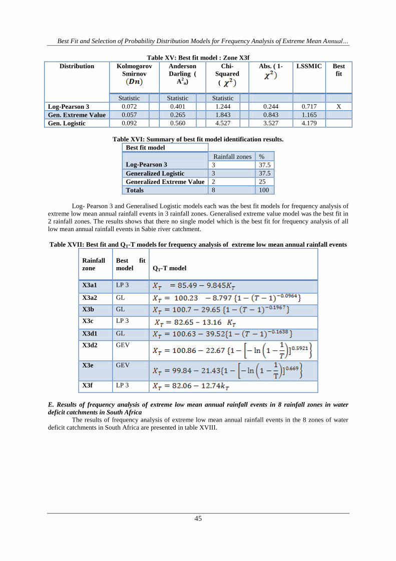
Best Fit and Selection of Probability Distribution Models for Frequency Analysis of Extreme Mean Annualhellip
47
Limitation of Criterion of Optimality
CMIC and LSSMIC have been developed in such a way that other parameters can be included This approach
ensures that technical and social parameters or variables can be included when needed In this particular case
peaks under threshold models have been included This could practically be assigned to the demand for water
resources needed at catchment level
Limitation of small sample and extreme events
This limitation is deemed to be solved by including Anderson-Darling and Kolomogrov-Smirnov in LSSMIC as
both cater for small sample and extreme events scenarios
IV CONCLUSION The main objective of this study was to develop two model identification criteria for frequency
analysis of extreme low mean rainfall events in water deficit catchments in South Africa The two model
selection criteria which were developed are
1 Candidate Model Identification Criterion (CM1C) for identifying candidate models
2 Least Sum of Statistics Model Identification Criterion ( LSSM1C) for identifying the best fit models for
frequency analysis of the extreme low mean annual rainfall events from the identified candidate models
The two developed criteria were applied to identify candidate models and best fit models for frequency analyses
of the extreme low mean annual rainfall events in 8 rainfall zones in Sabie river catchment Results obtained
showed that there no single probability distribution function is the best fit for all the 8 rainfall zones (table XVI)
Log-Pearson 3 (LP3) probability distribution function has been recommended for design hydro-
meteorological events mostly flood and drought in South Africa (Alexander 1990 2001) From the results of
this study Log-Pearson 3 may not be the only best fit model for frequency analyses of extreme hydro-
meteorological events in South Africa It is therefore important to carry out model identification processes to
identify best fit model for the specific required frequency analysis
Probability-Probability (P-P) plots were applied to evaluate the performance of CMIC and LSSMISC
The plots showed that CMIC and LSSMIC performed fairly well Although the Probability-Probability (P-P)
plot results cannot be considered completely conclusive CMIC and LSSMSC criteria make useful tools as
model selection method for frequency analysis of extreme mean annual rainfall events
ACKNOWLEDGEMENT The study has been supported by the Provincial Dept of Agriculture Rural Development Land and
Environmental Affairs Mpumalanga Provincial Government South Africa
REFERENCES [1] Akaike H 1974`` A new look at the statistical model identificationrsquorsquoIEEE Transaction on automatic
control vol 6 pp 716-725
[2] Alexander WJR 1990 Flood Hydrology for Southern Africa SANCOLD Pretoria RSA
[3] Alexander WJR 2001 Flood Risk Reduction Measures University of Pretoria Pretoria RSA
[4] Alexander WJR 2002a The standard design flood Journal of the South Africa Institution of Civil
[5] Engineers 44 (1)26-31
[6] Anderson TW Darling DA 1952 Asymptotic theory of certain goodness-of-fit criteria based on
[7] stochastic processes AnnMatStat 23 193-212
[8] AndersonD R and Burnham K P 2002 Avoiding pitfalls when using information-theoretic
methods Journal of wildlife management 66(3) 912-918
[9] Beven K J 2000 Rain-Run-off modeling The Primer John Wiley and sons Chichester UK 360
360pp
[10] Bobee B and Rasmussen P F 1995 Recent advances in flood frequency analysis Reviews of
Geophysics supplement July 1111-1116
[11] Bodini A and Cossu Q A 2010 Vulnerability assessment of Central-East Sardinia ( Italy) to
extreme rainfall events Journal of Natural hazards and Earth systems sciences 10 Pp 61-77
[12] Claeskens G Hjort NL 2003 The focused Information Criterion Journal of the American statistical
[13] Association 98 900-916
[14] FeyenHMJ 1970 Identification of run-off processes in catchments with a small scale topograph
[15] Furrer E M and Katz R W 2008 ``Improving the simulation of extreme precipitation events by
stochastic weather generatorsrsquorsquo Water Resources Research 44 W 12439doi 10292008 WR 007316
2008
[16] Gericke OJ 2010 Evaluation of the SDF method using a customized Design Flood Estimation Tool
University of Stellenbosch Stellenbosch South Africa 480 pp
Best Fit and Selection of Probability Distribution Models for Frequency Analysis of Extreme Mean Annualhellip
48
[17] Gorgens A H M Joint Peak- Volume ( JPV) Design Flood Hydrographs for South Africa WRC
Report 1420307 Water Research Commission Pretoria South Africa
[18] Gorgens A H M LysonsS Hayes L Makhabana M and Maluleke D 2007 Modernised South
African Design Floo Pro actce in the context of Dam safety WRC Report 1420 2 07 Water
Research omission Pretoria South Africa
[19] Goswani P and Ramesh K V 2007 Extreme rainfall events Vulnerability Analysis for Disaster
Management and Observation Systems Design Research Report CSIR PP21
[20] Hernandez A R P Balling R C Jr and Barber-Matinez 2009 Comparative analysis of indices of
extreme rainfall events Variation and trend from Southern Mexico Journal de Atmosfera 2 pages 219-
228
[21] Hosking JRM 1990 L-moments Analysis and estimation of distribution using Linear combinations
of
[22] order statistics Journal of the Royal statistics society Series B 52 105-124
[23] Hosking JRM Wallis JR Wood EF 1985 Estimation of the generalized extreme-value
distribution
[24] by the method of probability-weighted moments Technimetrics 27 (3) pp 251-261
[25] Hjort NL Claeskens G 2003 Rejoinder to the focused
[26] Jiang J 2014 The fence method Advances in statistics Volume 2014 Article ID 38081
[27] Kidson R Richards KS Carling PA 2005 Reconstructing the Ca-100 year flood in Northern
[28] Thailand Geomorphology 70 (2-4) 279-595
[29] Kottegoda NT Rosso R 1998 Statistics Probability and Reliability for Civil and Environmental
[30] Engineers McGrawHill New York
[31] Laio etal 2009 Model selection techniques for the frequency analysis of hydrological extremes
water
[32] Research Vol45 W07416
[33] Laio F 2004 Cramer-Von Mises and Anderson-Darling goodness-of-fit tests for extreme value
[34] distributions with unknown parameters Water Resources Research 40 W09308
[35] doi1010292004WR003204
[36] Mathwave(2011) httpwwwmathwavecom
[37] Mallows CL 1995 Some comments on Cp Technimetrics 37 362-372
[38] Mallows CL 1973 Some comments on Cp Technimetrics 15 661-675
[39] Meiz R and Bloschl G 2004 Regionaliisation of catchment model parameters J Hydrol 287 pp 95-
123
[40] Mkhandi SH Kachroo RK Gunasekara TAG 2000 Flood frequency analysis of Southern
Africa
[41] II Identification of regional distributions Hydrological Sciences Journal 45(3)449-464
[42] Mutua FM 1994 The use of the Akaike Information Criterion in the identification of an optimum
flood
[43] frequency model Hydro SciJ39 (3) 235-244
[44] Salami A W ( 2004) Prediction of the annual flow regime along Asa River using probability
distribution models AMSE periodicals Lyon France Modeling c-2004 65 (2) 41-56 ( httpamse-
modelingorgcontentamse 2004 htm)
[45] Schwarz G 1978 Estimating the dimension of a model Annals stat 6 461-464
[46] Schulze RE 1989 Non-stationary catchment responses and other problems in determing flood
series A case for a simulation modeling approach In Kienzle S W Maaren H (Eds) Proceedings
of the Fourth South African National Hyrological Symposium SANCIAHS Pretoria RSA pp 135-157
[47] ShamirE 2005 2004Application of temporal streamflow descriptors in hydrologic model parameter
estimationWater Resource Research 41 doi 10 10292004 WR 003409 SSN 0043-1397
[48] Shao J Sitter RR 1996 Bootstrip for imprinted Survey data Journal of the American statistical
[49] Association 93 819-831
[50] Smithers JC Schulze RE 2001 Design runoff estimation A review with reference to practices in
[51] South Africa Proceedings of Tenth South Africa National Hydrology Symposium 26-28 September
[52] 2001 School of BEEH University of Natal Pietermaritzburg RSA
[53] Smithers JC Schulze RE 2003 Design rainfall and flood estimation in South AfricaWRC Report
No
[54] 10600103 Water Research Commission Pretoria RSA
[55] Stedinger JR Vogel RM Foufoula E 1993 Frequency analysis of extreme events in Handbook
of
[56] Hydrology DR McGrawHill chap 18 66pp
Best Fit and Selection of Probability Distribution Models for Frequency Analysis of Extreme Mean Annualhellip
49
[57] Stedinger JR 1980 Fitting log normal distribution to hydrologic data Water Resource research
16(3)
[58] pp 481-490
[59] Stephens MA 1976 Asymptotic results for goodness-of-fit statistics with unknown parameters Ann
[60] Stat Vol 4 357-369
[61] Van der Linde A 2005 DIC in variable selection statistical Neerlandica 59 45-56
[62] Van der Linde A 2004 DIC in variable selection Technical report Institute of statistics University of
[63] Bremen httpwwwmathuni-bremende$simsard1downloadpapersvarse12pdf
[64] Wellner JA 1977 Aglirenko-Cantelli Theorem and strong laws of large numbers for function of
order
[65] statistics The annual of statistics vol5 number 3 1977 473-480
[66] Wilks DS 1998 Multi-site generalization of daily stochastic precipitation model J Hydro 210 178-
191
[67] Willens P Olsson J Ambjerg_Nielsen BeechamS Pathirana A BulowGregersen MadsenH and
Nguyen VTV 2007 Impact of climate change on rainfall extreme and urban drainage systems pp19-
20
[68] WMO- World Meteorological organization 1988 Analysing long Time Series of Hydrological data
with respect of climat variability WCAP-No 3 WMO-TD No 224
[69] WMO- World Meteorological organization 2009 Guidelines on Analysis of extremes in a changing
climate in support of informed decisions for adaptations WCDMP-No 72 WMO-TD No 1500
[70] Yua-Ping Xu Booij Martin J Tong Yang_Bin 2010 Uncertainity analysis in statistical modeling of
extreme hydrological events
[71] Yue S and Wang 2004 The Mann-Kendall test modified by effective sample size to detect trend in
serially correlated hydrological series Journal of Water Resources Management 18 Pages 201-218
Appendix A Probability-Probability (P-P) plots for extreme low mean rainfall events for the
8 rainfall zones
P-P Plot Zone X3a1
Gen Extreme Value Gen Logistic Log-Pearson 3
P (Empirical)
1090807060504030201
P (
Mo
de
l)
1
09
08
07
06
05
04
03
02
01
0
Fig 1 P-P plot Zone x3a1 Extreme mean annual rainfall events
Best Fit and Selection of Probability Distribution Models for Frequency Analysis of Extreme Mean Annualhellip
50
P-P Plot Zone x3a2
Gen Extreme Value Gen Logistic Log-Pearson 3
P (Empirical)
1090807060504030201
P (
Mo
de
l)
1
09
08
07
06
05
04
03
02
01
0
Fig 2 P-P plot Zone x3a2 Extreme mean annual rainfall events
P-P Plot Zone x3b
Gen Logistic Log-Pearson 3 Wakeby
P (Empirical)
1090807060504030201
P (
Model)
1
09
08
07
06
05
04
03
02
01
0
Fig 3 P-P plot Zone x3b Extreme mean annual rainfall events
Best Fit and Selection of Probability Distribution Models for Frequency Analysis of Extreme Mean Annualhellip
51
P-P Plot Zone x3c
Gen Extreme Value Gen Logistic Log-Pearson 3
P (Empirical)
10908070605040302010
P (
Model)
1
09
08
07
06
05
04
03
02
01
0
Fig4 P-P plot Zone x3c Extreme mean annual rainfall events
P-P Plot Zone x3d1
Gen Extreme Value Gen Logistic Wakeby
P (Empirical)
10908070605040302010
P (
Model)
1
09
08
07
06
05
04
03
02
01
0
Fig 5 P-P plot Zone x3d1 Extreme mean annual rainfall events
Best Fit and Selection of Probability Distribution Models for Frequency Analysis of Extreme Mean Annualhellip
52
P-P Plot Zone x3d2
Gen Extreme Value Gen Logistic Log-Pearson 3
P (Empirical)
1090807060504030201
P (
Model)
1
09
08
07
06
05
04
03
02
01
0
FIG 6 P-P plot Zone x3d2 Extreme mean annual rainfall events
P-P Plot Zone x3e
Gen Extreme Value Gen Logistic Log-Pearson 3
P (Empirical)
1080604020
P (
Model)
1
09
08
07
06
05
04
03
02
01
0
Fig 7 P-P plot Zone x3e Extreme mean annual rainfall events
Best Fit and Selection of Probability Distribution Models for Frequency Analysis of Extreme Mean Annualhellip
53
P-P Plot Zone x3f
Gen Extreme Value Gen Logistic Log-Pearson 3
P (Empirical)
1090807060504030201
P (
Mo
de
l)
1
09
08
07
06
05
04
03
02
01
0
Fig8 P-P plot Zone x3f Extreme mean annual rainfall events
Best Fit and Selection of Probability Distribution Models for Frequency Analysis of Extreme Mean Annualhellip
48
[17] Gorgens A H M Joint Peak- Volume ( JPV) Design Flood Hydrographs for South Africa WRC
Report 1420307 Water Research Commission Pretoria South Africa
[18] Gorgens A H M LysonsS Hayes L Makhabana M and Maluleke D 2007 Modernised South
African Design Floo Pro actce in the context of Dam safety WRC Report 1420 2 07 Water
Research omission Pretoria South Africa
[19] Goswani P and Ramesh K V 2007 Extreme rainfall events Vulnerability Analysis for Disaster
Management and Observation Systems Design Research Report CSIR PP21
[20] Hernandez A R P Balling R C Jr and Barber-Matinez 2009 Comparative analysis of indices of
extreme rainfall events Variation and trend from Southern Mexico Journal de Atmosfera 2 pages 219-
228
[21] Hosking JRM 1990 L-moments Analysis and estimation of distribution using Linear combinations
of
[22] order statistics Journal of the Royal statistics society Series B 52 105-124
[23] Hosking JRM Wallis JR Wood EF 1985 Estimation of the generalized extreme-value
distribution
[24] by the method of probability-weighted moments Technimetrics 27 (3) pp 251-261
[25] Hjort NL Claeskens G 2003 Rejoinder to the focused
[26] Jiang J 2014 The fence method Advances in statistics Volume 2014 Article ID 38081
[27] Kidson R Richards KS Carling PA 2005 Reconstructing the Ca-100 year flood in Northern
[28] Thailand Geomorphology 70 (2-4) 279-595
[29] Kottegoda NT Rosso R 1998 Statistics Probability and Reliability for Civil and Environmental
[30] Engineers McGrawHill New York
[31] Laio etal 2009 Model selection techniques for the frequency analysis of hydrological extremes
water
[32] Research Vol45 W07416
[33] Laio F 2004 Cramer-Von Mises and Anderson-Darling goodness-of-fit tests for extreme value
[34] distributions with unknown parameters Water Resources Research 40 W09308
[35] doi1010292004WR003204
[36] Mathwave(2011) httpwwwmathwavecom
[37] Mallows CL 1995 Some comments on Cp Technimetrics 37 362-372
[38] Mallows CL 1973 Some comments on Cp Technimetrics 15 661-675
[39] Meiz R and Bloschl G 2004 Regionaliisation of catchment model parameters J Hydrol 287 pp 95-
123
[40] Mkhandi SH Kachroo RK Gunasekara TAG 2000 Flood frequency analysis of Southern
Africa
[41] II Identification of regional distributions Hydrological Sciences Journal 45(3)449-464
[42] Mutua FM 1994 The use of the Akaike Information Criterion in the identification of an optimum
flood
[43] frequency model Hydro SciJ39 (3) 235-244
[44] Salami A W ( 2004) Prediction of the annual flow regime along Asa River using probability
distribution models AMSE periodicals Lyon France Modeling c-2004 65 (2) 41-56 ( httpamse-
modelingorgcontentamse 2004 htm)
[45] Schwarz G 1978 Estimating the dimension of a model Annals stat 6 461-464
[46] Schulze RE 1989 Non-stationary catchment responses and other problems in determing flood
series A case for a simulation modeling approach In Kienzle S W Maaren H (Eds) Proceedings
of the Fourth South African National Hyrological Symposium SANCIAHS Pretoria RSA pp 135-157
[47] ShamirE 2005 2004Application of temporal streamflow descriptors in hydrologic model parameter
estimationWater Resource Research 41 doi 10 10292004 WR 003409 SSN 0043-1397
[48] Shao J Sitter RR 1996 Bootstrip for imprinted Survey data Journal of the American statistical
[49] Association 93 819-831
[50] Smithers JC Schulze RE 2001 Design runoff estimation A review with reference to practices in
[51] South Africa Proceedings of Tenth South Africa National Hydrology Symposium 26-28 September
[52] 2001 School of BEEH University of Natal Pietermaritzburg RSA
[53] Smithers JC Schulze RE 2003 Design rainfall and flood estimation in South AfricaWRC Report
No
[54] 10600103 Water Research Commission Pretoria RSA
[55] Stedinger JR Vogel RM Foufoula E 1993 Frequency analysis of extreme events in Handbook
of
[56] Hydrology DR McGrawHill chap 18 66pp
Best Fit and Selection of Probability Distribution Models for Frequency Analysis of Extreme Mean Annualhellip
49
[57] Stedinger JR 1980 Fitting log normal distribution to hydrologic data Water Resource research
16(3)
[58] pp 481-490
[59] Stephens MA 1976 Asymptotic results for goodness-of-fit statistics with unknown parameters Ann
[60] Stat Vol 4 357-369
[61] Van der Linde A 2005 DIC in variable selection statistical Neerlandica 59 45-56
[62] Van der Linde A 2004 DIC in variable selection Technical report Institute of statistics University of
[63] Bremen httpwwwmathuni-bremende$simsard1downloadpapersvarse12pdf
[64] Wellner JA 1977 Aglirenko-Cantelli Theorem and strong laws of large numbers for function of
order
[65] statistics The annual of statistics vol5 number 3 1977 473-480
[66] Wilks DS 1998 Multi-site generalization of daily stochastic precipitation model J Hydro 210 178-
191
[67] Willens P Olsson J Ambjerg_Nielsen BeechamS Pathirana A BulowGregersen MadsenH and
Nguyen VTV 2007 Impact of climate change on rainfall extreme and urban drainage systems pp19-
20
[68] WMO- World Meteorological organization 1988 Analysing long Time Series of Hydrological data
with respect of climat variability WCAP-No 3 WMO-TD No 224
[69] WMO- World Meteorological organization 2009 Guidelines on Analysis of extremes in a changing
climate in support of informed decisions for adaptations WCDMP-No 72 WMO-TD No 1500
[70] Yua-Ping Xu Booij Martin J Tong Yang_Bin 2010 Uncertainity analysis in statistical modeling of
extreme hydrological events
[71] Yue S and Wang 2004 The Mann-Kendall test modified by effective sample size to detect trend in
serially correlated hydrological series Journal of Water Resources Management 18 Pages 201-218
Appendix A Probability-Probability (P-P) plots for extreme low mean rainfall events for the
8 rainfall zones
P-P Plot Zone X3a1
Gen Extreme Value Gen Logistic Log-Pearson 3
P (Empirical)
1090807060504030201
P (
Mo
de
l)
1
09
08
07
06
05
04
03
02
01
0
Fig 1 P-P plot Zone x3a1 Extreme mean annual rainfall events
Best Fit and Selection of Probability Distribution Models for Frequency Analysis of Extreme Mean Annualhellip
50
P-P Plot Zone x3a2
Gen Extreme Value Gen Logistic Log-Pearson 3
P (Empirical)
1090807060504030201
P (
Mo
de
l)
1
09
08
07
06
05
04
03
02
01
0
Fig 2 P-P plot Zone x3a2 Extreme mean annual rainfall events
P-P Plot Zone x3b
Gen Logistic Log-Pearson 3 Wakeby
P (Empirical)
1090807060504030201
P (
Model)
1
09
08
07
06
05
04
03
02
01
0
Fig 3 P-P plot Zone x3b Extreme mean annual rainfall events
Best Fit and Selection of Probability Distribution Models for Frequency Analysis of Extreme Mean Annualhellip
51
P-P Plot Zone x3c
Gen Extreme Value Gen Logistic Log-Pearson 3
P (Empirical)
10908070605040302010
P (
Model)
1
09
08
07
06
05
04
03
02
01
0
Fig4 P-P plot Zone x3c Extreme mean annual rainfall events
P-P Plot Zone x3d1
Gen Extreme Value Gen Logistic Wakeby
P (Empirical)
10908070605040302010
P (
Model)
1
09
08
07
06
05
04
03
02
01
0
Fig 5 P-P plot Zone x3d1 Extreme mean annual rainfall events
Best Fit and Selection of Probability Distribution Models for Frequency Analysis of Extreme Mean Annualhellip
52
P-P Plot Zone x3d2
Gen Extreme Value Gen Logistic Log-Pearson 3
P (Empirical)
1090807060504030201
P (
Model)
1
09
08
07
06
05
04
03
02
01
0
FIG 6 P-P plot Zone x3d2 Extreme mean annual rainfall events
P-P Plot Zone x3e
Gen Extreme Value Gen Logistic Log-Pearson 3
P (Empirical)
1080604020
P (
Model)
1
09
08
07
06
05
04
03
02
01
0
Fig 7 P-P plot Zone x3e Extreme mean annual rainfall events
Best Fit and Selection of Probability Distribution Models for Frequency Analysis of Extreme Mean Annualhellip
53
P-P Plot Zone x3f
Gen Extreme Value Gen Logistic Log-Pearson 3
P (Empirical)
1090807060504030201
P (
Mo
de
l)
1
09
08
07
06
05
04
03
02
01
0
Fig8 P-P plot Zone x3f Extreme mean annual rainfall events

Best Fit and Selection of Probability Distribution Models for Frequency Analysis of Extreme Mean Annualhellip
49
[57] Stedinger JR 1980 Fitting log normal distribution to hydrologic data Water Resource research
16(3)
[58] pp 481-490
[59] Stephens MA 1976 Asymptotic results for goodness-of-fit statistics with unknown parameters Ann
[60] Stat Vol 4 357-369
[61] Van der Linde A 2005 DIC in variable selection statistical Neerlandica 59 45-56
[62] Van der Linde A 2004 DIC in variable selection Technical report Institute of statistics University of
[63] Bremen httpwwwmathuni-bremende$simsard1downloadpapersvarse12pdf
[64] Wellner JA 1977 Aglirenko-Cantelli Theorem and strong laws of large numbers for function of
order
[65] statistics The annual of statistics vol5 number 3 1977 473-480
[66] Wilks DS 1998 Multi-site generalization of daily stochastic precipitation model J Hydro 210 178-
191
[67] Willens P Olsson J Ambjerg_Nielsen BeechamS Pathirana A BulowGregersen MadsenH and
Nguyen VTV 2007 Impact of climate change on rainfall extreme and urban drainage systems pp19-
20
[68] WMO- World Meteorological organization 1988 Analysing long Time Series of Hydrological data
with respect of climat variability WCAP-No 3 WMO-TD No 224
[69] WMO- World Meteorological organization 2009 Guidelines on Analysis of extremes in a changing
climate in support of informed decisions for adaptations WCDMP-No 72 WMO-TD No 1500
[70] Yua-Ping Xu Booij Martin J Tong Yang_Bin 2010 Uncertainity analysis in statistical modeling of
extreme hydrological events
[71] Yue S and Wang 2004 The Mann-Kendall test modified by effective sample size to detect trend in
serially correlated hydrological series Journal of Water Resources Management 18 Pages 201-218
Appendix A Probability-Probability (P-P) plots for extreme low mean rainfall events for the
8 rainfall zones
P-P Plot Zone X3a1
Gen Extreme Value Gen Logistic Log-Pearson 3
P (Empirical)
1090807060504030201
P (
Mo
de
l)
1
09
08
07
06
05
04
03
02
01
0
Fig 1 P-P plot Zone x3a1 Extreme mean annual rainfall events
Best Fit and Selection of Probability Distribution Models for Frequency Analysis of Extreme Mean Annualhellip
50
P-P Plot Zone x3a2
Gen Extreme Value Gen Logistic Log-Pearson 3
P (Empirical)
1090807060504030201
P (
Mo
de
l)
1
09
08
07
06
05
04
03
02
01
0
Fig 2 P-P plot Zone x3a2 Extreme mean annual rainfall events
P-P Plot Zone x3b
Gen Logistic Log-Pearson 3 Wakeby
P (Empirical)
1090807060504030201
P (
Model)
1
09
08
07
06
05
04
03
02
01
0
Fig 3 P-P plot Zone x3b Extreme mean annual rainfall events
Best Fit and Selection of Probability Distribution Models for Frequency Analysis of Extreme Mean Annualhellip
51
P-P Plot Zone x3c
Gen Extreme Value Gen Logistic Log-Pearson 3
P (Empirical)
10908070605040302010
P (
Model)
1
09
08
07
06
05
04
03
02
01
0
Fig4 P-P plot Zone x3c Extreme mean annual rainfall events
P-P Plot Zone x3d1
Gen Extreme Value Gen Logistic Wakeby
P (Empirical)
10908070605040302010
P (
Model)
1
09
08
07
06
05
04
03
02
01
0
Fig 5 P-P plot Zone x3d1 Extreme mean annual rainfall events
Best Fit and Selection of Probability Distribution Models for Frequency Analysis of Extreme Mean Annualhellip
52
P-P Plot Zone x3d2
Gen Extreme Value Gen Logistic Log-Pearson 3
P (Empirical)
1090807060504030201
P (
Model)
1
09
08
07
06
05
04
03
02
01
0
FIG 6 P-P plot Zone x3d2 Extreme mean annual rainfall events
P-P Plot Zone x3e
Gen Extreme Value Gen Logistic Log-Pearson 3
P (Empirical)
1080604020
P (
Model)
1
09
08
07
06
05
04
03
02
01
0
Fig 7 P-P plot Zone x3e Extreme mean annual rainfall events
Best Fit and Selection of Probability Distribution Models for Frequency Analysis of Extreme Mean Annualhellip
53
P-P Plot Zone x3f
Gen Extreme Value Gen Logistic Log-Pearson 3
P (Empirical)
1090807060504030201
P (
Mo
de
l)
1
09
08
07
06
05
04
03
02
01
0
Fig8 P-P plot Zone x3f Extreme mean annual rainfall events
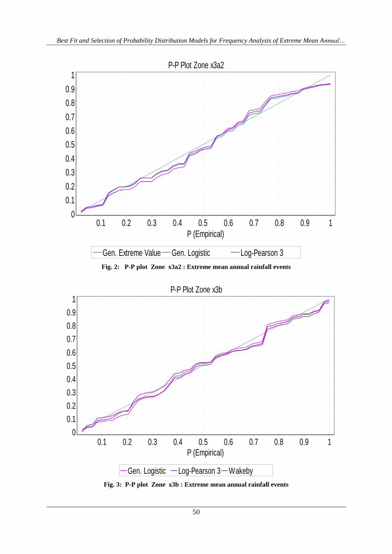
Best Fit and Selection of Probability Distribution Models for Frequency Analysis of Extreme Mean Annualhellip
50
P-P Plot Zone x3a2
Gen Extreme Value Gen Logistic Log-Pearson 3
P (Empirical)
1090807060504030201
P (
Mo
de
l)
1
09
08
07
06
05
04
03
02
01
0
Fig 2 P-P plot Zone x3a2 Extreme mean annual rainfall events
P-P Plot Zone x3b
Gen Logistic Log-Pearson 3 Wakeby
P (Empirical)
1090807060504030201
P (
Model)
1
09
08
07
06
05
04
03
02
01
0
Fig 3 P-P plot Zone x3b Extreme mean annual rainfall events
Best Fit and Selection of Probability Distribution Models for Frequency Analysis of Extreme Mean Annualhellip
51
P-P Plot Zone x3c
Gen Extreme Value Gen Logistic Log-Pearson 3
P (Empirical)
10908070605040302010
P (
Model)
1
09
08
07
06
05
04
03
02
01
0
Fig4 P-P plot Zone x3c Extreme mean annual rainfall events
P-P Plot Zone x3d1
Gen Extreme Value Gen Logistic Wakeby
P (Empirical)
10908070605040302010
P (
Model)
1
09
08
07
06
05
04
03
02
01
0
Fig 5 P-P plot Zone x3d1 Extreme mean annual rainfall events
Best Fit and Selection of Probability Distribution Models for Frequency Analysis of Extreme Mean Annualhellip
52
P-P Plot Zone x3d2
Gen Extreme Value Gen Logistic Log-Pearson 3
P (Empirical)
1090807060504030201
P (
Model)
1
09
08
07
06
05
04
03
02
01
0
FIG 6 P-P plot Zone x3d2 Extreme mean annual rainfall events
P-P Plot Zone x3e
Gen Extreme Value Gen Logistic Log-Pearson 3
P (Empirical)
1080604020
P (
Model)
1
09
08
07
06
05
04
03
02
01
0
Fig 7 P-P plot Zone x3e Extreme mean annual rainfall events
Best Fit and Selection of Probability Distribution Models for Frequency Analysis of Extreme Mean Annualhellip
53
P-P Plot Zone x3f
Gen Extreme Value Gen Logistic Log-Pearson 3
P (Empirical)
1090807060504030201
P (
Mo
de
l)
1
09
08
07
06
05
04
03
02
01
0
Fig8 P-P plot Zone x3f Extreme mean annual rainfall events
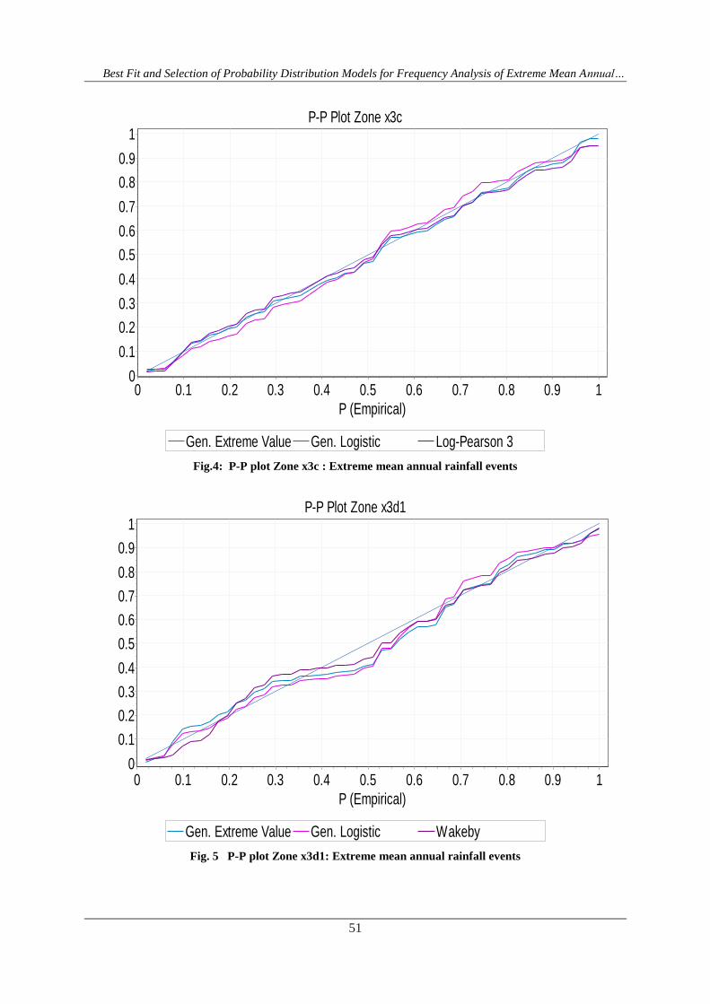
Best Fit and Selection of Probability Distribution Models for Frequency Analysis of Extreme Mean Annualhellip
52
P-P Plot Zone x3d2
Gen Extreme Value Gen Logistic Log-Pearson 3
P (Empirical)
1090807060504030201
P (
Model)
1
09
08
07
06
05
04
03
02
01
0
FIG 6 P-P plot Zone x3d2 Extreme mean annual rainfall events
P-P Plot Zone x3e
Gen Extreme Value Gen Logistic Log-Pearson 3
P (Empirical)
1080604020
P (
Model)
1
09
08
07
06
05
04
03
02
01
0
Fig 7 P-P plot Zone x3e Extreme mean annual rainfall events
Best Fit and Selection of Probability Distribution Models for Frequency Analysis of Extreme Mean Annualhellip
53
P-P Plot Zone x3f
Gen Extreme Value Gen Logistic Log-Pearson 3
P (Empirical)
1090807060504030201
P (
Mo
de
l)
1
09
08
07
06
05
04
03
02
01
0
Fig8 P-P plot Zone x3f Extreme mean annual rainfall events
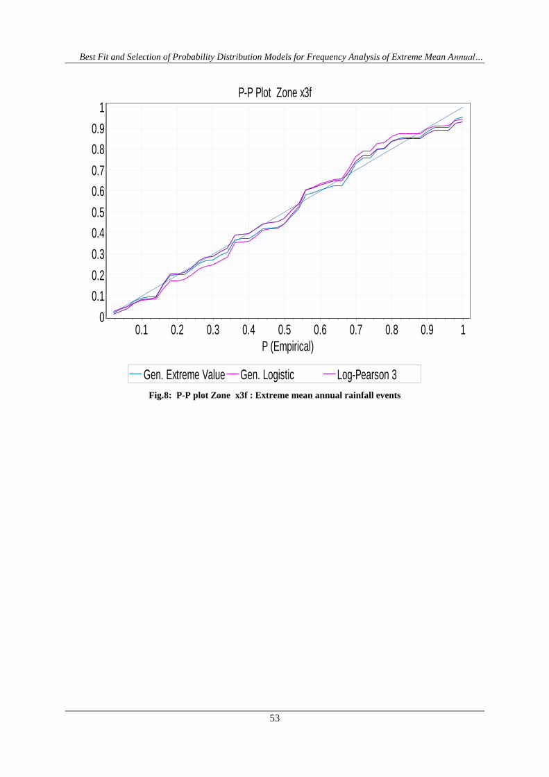
Best Fit and Selection of Probability Distribution Models for Frequency Analysis of Extreme Mean Annualhellip
53
P-P Plot Zone x3f
Gen Extreme Value Gen Logistic Log-Pearson 3
P (Empirical)
1090807060504030201
P (
Mo
de
l)
1
09
08
07
06
05
04
03
02
01
0
Fig8 P-P plot Zone x3f Extreme mean annual rainfall events


![Analysis of Extreme Rainfall Events (Drought and Flood ... · used (31 years). The procedure used by McKee et al. [3] for fitting the rainfall data to a probability distribution function](https://static.fdocuments.us/doc/165x107/5e88048d310c55215038bc46/analysis-of-extreme-rainfall-events-drought-and-flood-used-31-years-the.jpg)