ME 201/MTH 281/ME400/CHE400Bessel Functions

1. IntroductionThis notebook has two purposes: to give a brief introduction to Bessel functions, and to illustrate how Mathe-

matica can be used in working with Bessel functions. We begin with a summary of the origin of Bessel's equation inour course.

By separating variables for the Laplace equation in cylindrical coordinates, we found solutions of the form

F(r)G(z)cosHmqL

sinHmqL ,

where m = 0, 1, 2, ... . The radial function F satisfied Bessel's equation of order m with a parameter l:

(1)d

drr

dF

dr+ lr -

m2

rF = 0 .

Here l is a constant arising in the separation process. By introducing a new independent variable

x = l r ,we may put equation (1) in the form

(2)d

dxx

dF

dx+ x -

m2

x= 0 .

We deal with the solutions of this equation for general m in section 3.

The important special case m = 0 corresponds to solutions of the Laplace equation which are independent of q.The equation for F then reduces to Bessel's equation of order 0:

(3)d

dxx

dF

dx+ xF = 0 .

We deal with solutions of this equation in section 2.

The equations (2) and (3) arise in those cases where the solution is oscillatory in r and exponential in z. Inother problems, the homogeneous boundary conditions are on surfaces of constant z, making the solutions oscillatoryin z. In those cases, the separation constant has a sign opposite to that in equation (1), and the resulting radial equationhas the form

(4)d

drr

dF

dr- lr +

m2

rF = 0 .

This is called the modified Bessel's equation of order m with a parameter l. The scaling x = l r reduces this to

(5)d

dxx

dF

dx- x +

m2

xF = 0 .

Solutions of this equation are discussed in section 5. The special case m = 0 for axisymmetric solutions is

(6)d

dxx

dF

dx- xF = 0 .

and solutions of this equation are discussed in section 4.

2. The Bessel Functions J0 and Y0ü 2.1 Summary of Solution by the Method of Frobenius

As shown in class, equation (3) has a regular singular point at x = 0, and therefore can be solved by the methodof Frobenius. The detailed calculations show that the indicial equation has a repeated root 0, 0. Thus there is only onesolution of the Frobenius form, and the second solution has a logarithmic singularity at x = 0. Because the indicialroot is 0, the Frobenius solution has the form of a power series and is thus well-behaved at x = 0. This solution hasbeen standardized by choosing the multiplicative constant so that the function value is 1 when x = 0. The resultingfunction is called the Bessel function of the first kind of order 0, and is denoted by J0. The second solution -- the onewith a logarithmic singularity at x = 0 -- has also been standardized, and it is denoted by Y0.

ü 2.2 Series Expansions for J0and Y0The Frobenius method readily yields the following series for J0:

(7)J0 HxL = 1 -Hx ê2L2

H1 !L2+

Hx ê2L4

H2 !L2-

Hx ê2L6

H3 !L2+ . . . = ‚

k=0

¶ H-1Lk Hx ê2L2 k

Hk !L2.

Because the equation has no other singular points, we expect this series to converge for all x, a conclusion easilyverified by the ratio test.

The derivation of a series for Y0HxL is much more difficult, and the resulting series is more complicated:

(8)Y0 HxL =2

p:ln K

1

2x + g> J0 HxL +

2

p:Hx ê2L2

H1 !L2- K1 +

1

2OHx ê2L4

H2 !L2+ K1 +

1

2+1

3OHx ê2L6

H3 !L2- . . .>

Here g is Euler's constant which is known to Mathematica by the name EulerGamma: N@EulerGammaD

0.577216

Fortunately for us, we do not have to use these series directly to get values for these functions. Bessel functions arebuilt-in to Mathematica, and we consider that next.

ü 2.3 Using Mathematica to Evaluate J0 and Y0The Mathematica function BesselJ[m,x] returns the value of JmHxL and the function BesselY[m,x] returns the

value of YmHxL. As an experiment, let's calculate the value of J0 for x = 1, 2, and 3, using both the series of equation (7)and the Mathematica function. We first define the Nth partial sum of the series. Jseries@x_, n_D := Sum@H-1L^k * Hx ê 2L^H2 * kL ê Hk!L^2, 8k, 0, n<D

We start with x = 1. Mathematica givesBesselJ@0, 1.0D

0.765198

The series gives Table@Jseries@1.0, nD, 8n, 1, 4<D

80.75, 0.765625, 0.765191, 0.765198<

2 bessfunc.nb

Thus four terms are sufficient to give six-place accuracy. For x = 2 and 3, we expect that we will need more terms inthe series.BesselJ@0, 2.0D

0.223891

Table@Jseries@2.0, nD, 8n, 4, 6<D

80.223958, 0.223889, 0.223891<

For x = 2, we see that 6 terms are sufficient for six-place accuracy.BesselJ@0, 3.0D

-0.260052

Table@Jseries@3.0, nD, 8n, 5, 7<D

8-0.260291, -0.260041, -0.260052<

For x = 3, we need 7 terms.

From here on, we will use the Mathematica built-in functions because they are much more convenient. In anycase, the series cannot be used for very large values of x, something which Mathematica knows to avoid.

At this point we have considerable machinery, but we have no intuitive feeling for Bessel functions. Weremedy that by looking at some graphs.

ü 2.4 Plots of J0 and Y0An appropriate size for printed graphs is 250. For display of graphs, a size of 350 is better. The size is

controlled throughout the notebook by the SetOption command below. After executing that, we use the function Plotto get some pictures of J0and Y0. First we plot J0.SetOptions@Plot, ImageSize Ø 250D;

graphJ0 = Plot@BesselJ@0, xD, 8x, 0, 20<, AxesLabel -> 8"x", "J0"<D

5 10 15 20x

-0.4

-0.2

0.2

0.4

0.6

0.8

1.0J0

An interesting graph. We see that J0 is an oscillatory function. In fact it looks a lot like a damped trig function, anobservation which we will make more precise in section 2.6. We also see that J0 has many zeros (in fact it hasinfinitely many). As we have already seen in class, we need to find these zeros to find the eigenvalues for solutions ofLaplace's equation by separation of variables. In section 2.5, we will see how to do this.

Now let's plot Y0. We will have to be a little careful because of the singularity at x = 0, so we start our plot alittle away from 0. Let's use the same plot range that Mathematica selected above for J0.

bessfunc.nb 3

graphY0 =Plot@BesselY@0, xD, 8x, 0.01, 20<, PlotRange -> 8-0.4, 1.0<, AxesLabel -> 8"x", "Y0"<D

5 10 15 20x

-0.4

-0.2

0.2

0.4

0.6

0.8

1.0Y0

The function Y0, like J0, is oscillatory, and again looks like a damped trig function, apart from the divergence to -¶ atx = 0. Let's plot the two functions on the same graph:Show@graphJ0, graphY0D

5 10 15 20x

-0.4

-0.2

0.2

0.4

0.6

0.8

1.0J0

Now we see that for larger x they look like damped trig functions differing only by a phase shift. We will see insection 2.6 the truth of that statement.

ü 2.5 Finding Roots of J0Earlier in our course, we have seen examples of finding roots by using FindRoot. That will also work for the

Bessel functions we are studying here. For J0, for example, we see from the graph that the first root is between 2 and3. Thus we can use FindRoot with an initial guess of 2.5:root1 = FindRoot@BesselJ@0, xD, 8x, 2.5<D

8x Ø 2.40483<

The answer is in the form of a replacement rule. Let's check it by evaluating J0 at that value:BesselJ@0, xD ê. root1

-9.51574 µ 10-17

That's close enough to zero for most purposes. We could continue finding the other roots of J0 by altering the initialguess and repeating the calculation. Fortunately, there is a much easier way in Mathematica. Mathematica has built-in functions for getting the zeros of Bessel functions. For the J Bessel function the name of the function returning azero is BesselJZero[n,k]. This returns the kth positive zero of Jn. For convenience we use this function to construct alist (Table) of the first 40 zeros of J0. We assign the list to zerolist.zerolist = N@Table@BesselJZero@0, iD, 8i, 1, 40<DD

82.40483, 5.52008, 8.65373, 11.7915, 14.9309, 18.0711, 21.2116, 24.3525, 27.4935, 30.6346,33.7758, 36.9171, 40.0584, 43.1998, 46.3412, 49.4826, 52.6241, 55.7655, 58.907, 62.0485,65.19, 68.3315, 71.473, 74.6145, 77.756, 80.8976, 84.0391, 87.1806, 90.3222, 93.4637,96.6053, 99.7468, 102.888, 106.03, 109.171, 112.313, 115.455, 118.596, 121.738, 124.879<

The zeros are then available for any subsequent calculation. For example, the first zero is given by

4 bessfunc.nb

root1 = zerolist@@1DD

2.40483

This is the same as the value found by FindRoot. As before, we check this by evaluating J0 for this value:BesselJ@0, xD ê. x -> root1

-9.51574 µ 10-17

We can learn something interesting about the zeros by calculating the spacing between successive zeros:Table@Hzerolist@@n + 1DD - zerolist@@nDDL, 8n, 1, 39<D

83.11525, 3.13365, 3.13781, 3.13938, 3.14015, 3.14057, 3.14083, 3.14101, 3.14113, 3.14121,3.14128, 3.14133, 3.14137, 3.1414, 3.14142, 3.14144, 3.14146, 3.14147, 3.14149, 3.1415,3.1415, 3.14151, 3.14152, 3.14152, 3.14153, 3.14153, 3.14154, 3.14154, 3.14155, 3.14155,3.14155, 3.14155, 3.14156, 3.14156, 3.14156, 3.14156, 3.14156, 3.14157, 3.14157<

We see that although the zeros are not exactly equally spaced, they are apparently asymptotically equally spaced, andthe spacing looks suspiciously like p! More on this later.

The main point in this section is that the roots of Bessel functions are easily and instantly available.

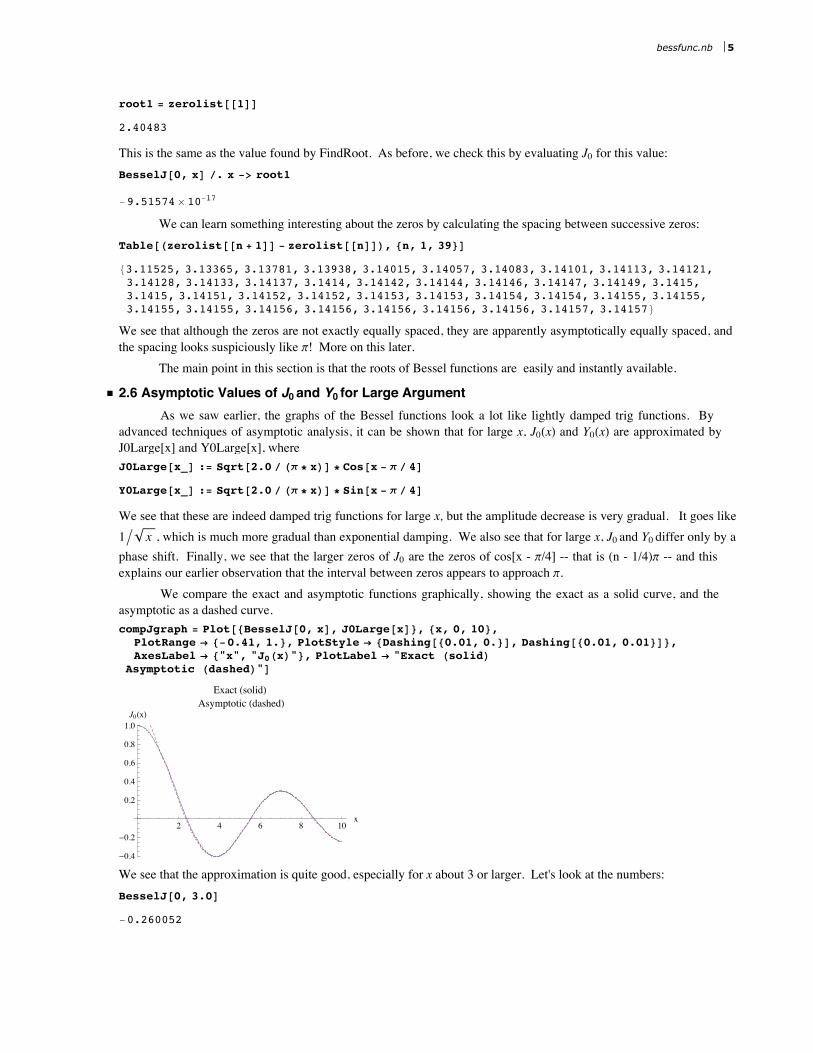
ü 2.6 Asymptotic Values of J0 and Y0 for Large ArgumentAs we saw earlier, the graphs of the Bessel functions look a lot like lightly damped trig functions. By

advanced techniques of asymptotic analysis, it can be shown that for large x, J0HxL and Y0HxL are approximated byJ0Large[x] and Y0Large[x], where J0Large@x_D := Sqrt@2.0 ê Hp * xLD * Cos@x - p ê 4D

Y0Large@x_D := Sqrt@2.0 ê Hp * xLD * Sin@x - p ê 4D

We see that these are indeed damped trig functions for large x, but the amplitude decrease is very gradual. It goes like1ë x , which is much more gradual than exponential damping. We also see that for large x, J0 and Y0 differ only by aphase shift. Finally, we see that the larger zeros of J0 are the zeros of cos[x - p/4] -- that is (n - 1/4)p -- and thisexplains our earlier observation that the interval between zeros appears to approach p.

We compare the exact and asymptotic functions graphically, showing the exact as a solid curve, and theasymptotic as a dashed curve.compJgraph = Plot@8BesselJ@0, xD, J0Large@xD<, 8x, 0, 10<,

PlotRange Ø 8-0.41, 1.<, PlotStyle Ø 8Dashing@80.01, 0.<D, Dashing@80.01, 0.01<D<,AxesLabel Ø 8"x", "J0HxL"<, PlotLabel Ø "Exact HsolidL

Asymptotic HdashedL"D

2 4 6 8 10x

-0.4

-0.2

0.2

0.4

0.6

0.8

1.0J0HxL

Exact HsolidLAsymptotic HdashedL

We see that the approximation is quite good, especially for x about 3 or larger. Let's look at the numbers:BesselJ@0, 3.0D

-0.260052

bessfunc.nb 5

J0Large@3.0D

-0.276507

There is roughly a 5% difference.

Finally, we compare graphically the exact and asymptotic forms for Y0:compYgraph = Plot@8BesselY@0, xD, Y0Large@xD<, 8x, 0.01, 10<,

PlotRange Ø 8-0.4, 1.<, PlotStyle Ø 8Dashing@80.01, 0.<D, Dashing@80.01, 0.01<D<,AxesLabel Ø 8"x", "Y0HxL"<, PlotLabel Ø "Exact HsolidL

Asymptotic HdashedL"D

2 4 6 8 10x

-0.4

-0.2

0.2

0.4

0.6

0.8

1.0Y0HxL

Exact HsolidLAsymptotic HdashedL

Again excellent agreement for x greater than about 3. Here are the numbers for x = 3:BesselY@0, 3.0D

0.37685

Y0Large@3.0D

0.368443

Only about a 2% difference.

3. The Bessel Functions Jm and Ymü 3.1 Summary of Solution by the Method of Frobenius

The functions JmHxL and YmHxL are the solutions of equation (2), which is Bessel's equation of order m. Asshown in class, equation (2) has a regular singular point at x = 0, and therefore can be solved by the method of Frobe-nius. The detailed calculations show that the indicial equation has roots -m, m. These differ by an integer, and so theFrobenius Theorem tells us that we will get a solution of the Frobenius form corresponding to the root +m, and thatthere is the possibility of a logarithmic singularity at x = 0 for the other solution. Detailed analysis confirms that thesecond solution is not of the Frobenius form and does indeed have a logarithmic singularity at x = 0. The Frobeniussolution is of the form of a power series times xm and is thus well-behaved at x = 0 (under the assumption madethroughout this notebook that m is a non-negative integer). This well-behaved solution, when standardized as insection 3.2, is called the Bessel function of the first kind of order m, and is denoted by JmHxL. The singular solution,standardized in section 3.2, is called the Bessel function of the second kind of order m, and is denoted by YmHxL.

ü 3.2 Series Expansions for Jm and YmThe Frobenius method readily yields a series for the solution associated with the indicial root +m. With the

multiplicative constant chosen in a standard way, this series becomes the function Jm:

(9)

Jm HxL =x

2

m 1

m !-

Hx ê2L2

H1 !L H1 + mL !+

Hx ê2L4

H2 !L H2 + mL !-

Hx ê2L6

H3 !L H3 + mL !+ . . .

6 bessfunc.nb

(9)

=x

2

m‚k=0

¶ H-1Lk Hx ê2L2 k

Hk !L Hk + mL !.

Because the equation has no other singular points, the series converges for all x, a conclusion easily verified by theratio test.

The derivation of a series for YmHxL is much more difficult, and the resulting series is complicated:

(10)Ym HxL = -

Hx ê2L-m

p‚k=0

m-1 Hm - k - 1L !

k !

x

2

2 k+

2

pln K

1

2x Jm HxL -

Hx ê2Lm

p‚k=0

¶

8y Hk + 1L + y Hm + k + 1L<H-1Lk Hx ê2L2 k

k ! Hm + kL !,

where y is the Digamma function, given by y(1) = -g (g is Euler's constant as before), and y(n) = -g + ⁄k=1n-11 êk.

Notice that the logarithm is not the worst singularity in Ym at x = 0. There are negative powers of x also, withthe highest being x-m.

We do not have to use these series directly because these functions are built in to Mathematica. We considerthat next.

ü 3.3 Using Mathematica to Evaluate Jm and YmThe Mathematica function BesselJ[m,x] returns the value of JmHxL and the function BesselY[m,x] returns the

value of YmHxL. As an experiment, let's calculate the value of Jm for x = 2, and for m = 1, 2, and 3, using both the seriesof equation (9) and Mathematica. We first define the Nth partial sum of the series. Jseries@x_, m_, n_D := Hx ê 2L^m * Sum@H-1L^k * Hx ê 2L^H2 * kL ê HHk!L * Hk + mL!L, 8k, 0, n<D

We start with m = 1. Mathematica givesBesselJ@1, 2.0D

0.576725

The series gives Table@Jseries@2.0, 1, nD, 8n, 1, 5<D

80.5, 0.583333, 0.576389, 0.576736, 0.576725<

Thus five terms are sufficient to give six-place accuracy for x = 2. Now we try m = 2.BesselJ@2, 2.0D

0.352834

Table@Jseries@2.0, 2, nD, 8n, 3, 6<D

80.352778, 0.352836, 0.352834, 0.352834<

Thus again five terms are sufficient for six-place accuracy for x = 2. Finally, we try m = 3.BesselJ@3, 2.0D

0.128943

Table@Jseries@2.0, 3, nD, 8n, 3, 6<D

80.128935, 0.128943, 0.128943, 0.128943<

Here four terms are sufficient.

From here on, we will use the Mathematica built-in functions because they are much more convenient. In anycase, the series can be used effectively only for moderately small values of »x».

bessfunc.nb 7

At this point, we don't have a good picture of how the Bessel functions depend on the order m. We next lookat some graphs to illustrate this.

ü 3.4 Plots of Jm and YmTo look at the dependence of Jm on the order m, we plot the first six Bessel functions over the x-range {0, 20}.

graphJm = Plot@8BesselJ@0, xD, BesselJ@1, xD, BesselJ@2, xD, BesselJ@3, xD, BesselJ@4, xD,BesselJ@5, xD<, 8x, 0, 20<, PlotRange Ø 8-0.41, 1.<, AxesLabel Ø 8"x", "Jm"<D

5 10 15 20x

-0.4

-0.2

0.2

0.4

0.6

0.8

1.0Jm

An interesting graph, although a little busy. The graph illustrates the fact that the larger m is, the more slowly theBessel function starts up. This happens because Jm is proportional to xm. Thus at x = 0, Jm and its first m - 1 deriva-tives vanish. After this initial sluggish start for the larger m's, we see that the Jm ' s have similar behavior -- that is, theyall look like damped trig functions (which we look at in more detail in section 3.6) and they all have infinitely manyzeros (which we learn how to find in section 3.5).

Now let's plot Ym. We will have to be a little careful because of the singularity at x = 0, so we start our plot alittle away from 0. Let's use the same m-values as above for the J's.graphYm = Plot@8BesselY@0, xD, BesselY@1, xD, BesselY@2, xD, BesselY@3, xD, BesselY@4, xD,

BesselY@5, xD<, 8x, 0.01`, 20<, PlotRange Ø 8-0.41, 1.<, AxesLabel Ø 8"x", "Jm"<D

5 10 15 20x

-0.4

-0.2

0.2

0.4

0.6

0.8

1.0Jm

The functions with the higher values of m diverge to infinity more rapidly as x Ø 0, because of the x-m term, and thismakes it easy to tell which curve is which on the graph. After the initial divergence, the Y's settle into the by-nowfamiliar damped oscillation. You may have noticed that the above graph took longer to produce than the previous onefor the J's. That's because the computational effort to find values of the Y's is much greater than that for finding the J's.

ü 3.5 Finding Roots of JmEarlier we found roots of J0. In the same way, we can find the roots of any Jm. As an example, let's find the

first 40 zeros of J5. zerolist = N@Table@BesselJZero@5, iD, 8i, 1, 40<DD

88.77148, 12.3386, 15.7002, 18.9801, 22.2178, 25.4303, 28.6266, 31.8117, 34.9888, 38.1599,41.3264, 44.4893, 47.6494, 50.8072, 53.963, 57.1173, 60.2702, 63.4221, 66.5729, 69.7229,72.8722, 76.0208, 79.1689, 82.3164, 85.4636, 88.6103, 91.7567, 94.9028, 98.0485, 101.194,104.339, 107.484, 110.629, 113.774, 116.918, 120.063, 123.207, 126.351, 129.495, 132.639<

The zeros are then available for any subsequent calculation. For example, the first zero is given by

8 bessfunc.nb

root1 = zerolist@@1DD

8.77148

We check this by evaluating J5 for this value:BesselJ@5, xD ê. x -> root1

6.54068 µ 10-15

Excellent accuracy. As we did before for J0, let's check the spacing between these zeros:Table@Hzerolist@@n + 1DD - zerolist@@nDDL, 8n, 1, 39<D

83.56712, 3.36157, 3.27996, 3.23767, 3.21254, 3.19628, 3.1851, 3.17706, 3.17109, 3.16651,3.16294, 3.16008, 3.15777, 3.15586, 3.15428, 3.15294, 3.15181, 3.15084, 3.15, 3.14927,3.14863, 3.14807, 3.14757, 3.14713, 3.14674, 3.14638, 3.14607, 3.14578, 3.14552, 3.14528,3.14506, 3.14487, 3.14469, 3.14452, 3.14437, 3.14422, 3.14409, 3.14397, 3.14386<

We see again that although the zeros are not exactly equally spaced, they seem to be approaching equal spacing for thelarge roots, and as before the spacing seems to be approaching p. More on this later.

From our graph earlier of Jm for m = 0, 1, 2, 3, 4, and 5, we would expect the first root of Jm to increase withm. Let's check this by finding the first root of each of the first 11 Bessel functions:N@Table@BesselJZero@m, 1D, 8m, 0, 10<DD

82.40483, 3.83171, 5.13562, 6.38016, 7.58834,8.77148, 9.93611, 11.0864, 12.2251, 13.3543, 14.4755<

Our expectation was correct.

As we saw before, the functions BesselJZero and BesselYZero make the roots of Bessel functions easily andinstantly available.

ü 3.6 Asymptotic Values of Jm and Ym for Large ArgumentThe asymptotic formulas we quoted earlier for J0and Y0 have extensions to Jm and Ym. It can be shown that for

large x, JmHxL and YmHxL are approximated by JLarge[m,x] and YLarge[m,x], where JLarge@m_, x_D := Sqrt@2.0 ê Hp * xLD * Cos@x - m * p ê 2 - p ê 4D

YLarge@m_, x_D := Sqrt@2.0 ê Hp * xLD * Sin@x - m * p ê 2 - p ê 4D

These formulas include J0 and Y0 as special cases. As before, we see that the amplitude decrease is very gradual. Itgoes like 1ë x and is much more gradual than exponential damping. We also see that for large x, Jm and Ym differonly by a phase shift. Finally, we see that the large zeros of Jm are the zeros of cos[x - mp/2 - p/4] -- that is (n + m/2 -1/4)p -- and this explains our earlier observation that the interval between zeros approachs p.

We compare the exact and asymptotic functions graphically, showing the exact as a solid curve, and theasymptotic as a dashed curve. By way of example, we do this for m = 5.

bessfunc.nb 9

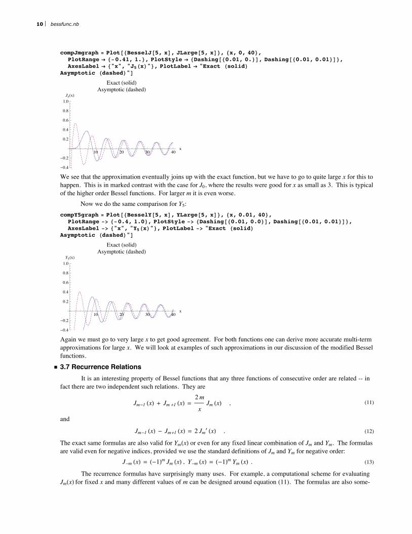
compJmgraph = Plot@8BesselJ@5, xD, JLarge@5, xD<, 8x, 0, 40<,PlotRange Ø 8-0.41, 1.<, PlotStyle Ø 8Dashing@80.01, 0.<D, Dashing@80.01, 0.01<D<,AxesLabel Ø 8"x", "J5HxL"<, PlotLabel Ø "Exact HsolidL

Asymptotic HdashedL"D

10 20 30 40x

-0.4

-0.2

0.2

0.4

0.6

0.8

1.0J5HxL

Exact HsolidLAsymptotic HdashedL

We see that the approximation eventually joins up with the exact function, but we have to go to quite large x for this tohappen. This is in marked contrast with the case for J0, where the results were good for x as small as 3. This is typicalof the higher order Bessel functions. For larger m it is even worse.

Now we do the same comparison for Y5:compY5graph = Plot@8BesselY@5, xD, YLarge@5, xD<, 8x, 0.01, 40<,

PlotRange -> 8-0.4, 1.0<, PlotStyle -> 8Dashing@80.01, 0.0<D, Dashing@80.01, 0.01<D<,AxesLabel -> 8"x", "Y5HxL"<, PlotLabel -> "Exact HsolidL

Asymptotic HdashedL"D

10 20 30 40x

-0.4

-0.2

0.2

0.4

0.6

0.8

1.0Y5HxL

Exact HsolidLAsymptotic HdashedL

Again we must go to very large x to get good agreement. For both functions one can derive more accurate multi-termapproximations for large x. We will look at examples of such approximations in our discussion of the modified Besselfunctions.

ü 3.7 Recurrence RelationsIt is an interesting property of Bessel functions that any three functions of consecutive order are related -- in

fact there are two independent such relations. They are

(11)Jm-1 HxL + Jm+1 HxL =2 m

xJm HxL ,

and

(12)Jm-1 HxL - Jm+1 HxL = 2 Jm£ HxL .

The exact same formulas are also valid for YmHxL or even for any fixed linear combination of Jm and Ym. The formulasare valid even for negative indices, provided we use the standard definitions of Jm and Ym for negative order:

(13)J-m HxL = H-1Lm Jm HxL , Y-m HxL = H-1Lm Ym HxL .

The recurrence formulas have surprisingly many uses. For example, a computational scheme for evaluatingJmHxL for fixed x and many different values of m can be designed around equation (11). The formulas are also some-times used in the evaluation of integrals involving Bessel functions, as we shall see in the next section.

10 bessfunc.nb

The recurrence formulas have surprisingly many uses. For example, a computational scheme for evaluatingJmHxL for fixed x and many different values of m can be designed around equation (11). The formulas are also some-times used in the evaluation of integrals involving Bessel functions, as we shall see in the next section.

ü 3.8 Integrals Involving Bessel FunctionsIn completing the solution of the Laplace and other equations by separation of variables in cylindrical coordi-

nates, one usually has to expand some boundary function in a series of Bessel functions. This in turn requires theevaluation of certain integrals involving the Bessel functions. With complicated boundary functions these integralsmust be done numerically, which is no problem in Mathematica with the NIntegrate function. For certain simple casesof boundary functions, the integrals can be done analytically, and these simple cases are often useful as test andcalibration cases for the numerical approach. We consider in this section two elementary integrals that can be doneanalytically.

For the first example, we start with the recurrence formulas (11) and (12). We multiply (11) by xm and (12) byxm and add them up. The result can be put into the form

d

dx@xm Jm HxLD = xm Jm-1 HxL ,

and by integrating this, we get the following indefinite integral:

(14)‡ xm Jm-1HxL „ x = xm JmHxL .

A frequently occuring special case is given by m = 1:

(15)‡ x J0HxL „ x = x J1HxL .

By integration-by-parts, we can parlay this into other integrals. For example,

Ÿ x3J0HxL„x

can be evaluated by letting u = x2 and dv = xJ0HxLdx, hence v = xJ1HxL. The integration-by-parts then gives

(16)‡ x3 J0HxL „ x = x3 J1HxL - 2 x2 J2HxL .

Mathematica knows how to do these integrals analytically. Consider the integral given in (15):Integrate@x * BesselJ@0, xD, xD

1

2x2 Hypergeometric0F1RegularizedB2, -

x2

4F

Not what we expected! Let's see what FullSimplify does for us.FullSimplify@%D

x BesselJ@1, xD

That's better.

Here is the Mathematica version of the integral in (16): Integrate@x^3 * BesselJ@0, xD, xD

-x2 H-2 BesselJ@2, xD + x BesselJ@3, xDL

By using equation (11), you can show that this is equivalent to equation (16).

4. The Bessel Functions I0 and K0The functions I0 and K0 considered in this section are solutions of equation (6), the modified Bessel's equation

of order 0. In principle, all of the development for J0 and Y0 could be repeated here with the minor variations requiredby the switch from J0 and Y0 to I0 and K0. In practice, the functions I0 and K0 are not used as much in our course as J0and Y0, so we will keep the discussion very brief.

bessfunc.nb 11

The functions I0 and K0 considered in this section are solutions of equation (6), the modified Bessel's equationof order 0. In principle, all of the development for J0 and Y0 could be repeated here with the minor variations requiredby the switch from J0 and Y0 to I0 and K0. In practice, the functions I0 and K0 are not used as much in our course as J0and Y0, so we will keep the discussion very brief.

The modified Bessel's equation has a regular singular point at x = 0. The application of the method of Frobe-nius shows that the indicial equation has repeated roots 0, 0, so there is one solution of the Frobenius form, and asecond solution with a logarithmic singularity. The solution well-behaved at x = 0 is standardized as I0HxL, and theFrobenius series is

(17)I0 HxL = 1 +Hx ê2L2

H1 !L2+

Hx ê2L4

H2 !L2+

Hx ê2L6

H3 !L2+ . . . = ‚

k=0

¶ Hx ê2L2 k

Hk !L2.

The series for the second solution K0 is more difficult to obtain and more intricate. It is given by

(18)K0 HxL = -:ln K1

2x + g> I0 HxL + :

Hx ê2L2

H1 !L2+ K1 +

1

2OHx ê2L4

H2 !L2+ K1 +

1

2+1

3OHx ê2L6

H3 !L2- . . . > .

These functions are both built in. The Mathematica function BesselI[0,x] gives I0HxL and the functionBesselK[0,x] gives K0HxL. Let's see what they look like. graphI0 = Plot@BesselI@0, xD, 8x, 0, 4<,

PlotRange Ø 880, 4<, 8-0.1, 11.5<<, AxesLabel -> 8"x", "I0HxL"<D

1 2 3 4x0

2

4

6

8

10

I0HxL

We see that I0 starts at 1 and appears to increase exponentially. Now we plot K0, avoiding the singularity at x = 0.graphK0 = Plot@BesselK@0, xD, 8x, 0.01, 4<, AxesLabel -> 8"x", "K0HxL"<D

1 2 3 4x

0.2

0.4

0.6

0.8

1.0

1.2

K0HxL

We see that K0 appears to drop exponentially. As with J0 and Y0, it is possible to derive simple asymptotic approxima-tions for large argument. One can show that for large x, I0HxL is approximated by I0Large[x], and that K0HxL is approxi-mated by K0Large[x], where I0Large@x_D := Exp@xD ê Sqrt@2 * p * xD

K0Large@x_D := Exp@-xD * Sqrt@p ê H2 * xLD

We compare the exact and asymptotic formulas graphically, starting with I0.

12 bessfunc.nb

compIgraph = Plot@8BesselI@0, xD, I0Large@xD<, 8x, 0.01, 4<,PlotRange -> 80, 15.0<, PlotStyle -> 8Dashing@0D, Dashing@80.01, 0.01<D<,AxesLabel -> 8"x", "I0HxL"<, PlotLabel -> "Exact HsolidL

Asymptotic HdashedL"D

0 1 2 3 4x

2

4

6

8

10

12

14

I0HxL

Exact HsolidLAsymptotic HdashedL

We see that the approximation is adequate although not spectacular. It is possible to develop more accurate approxima-tions which essentially provide a small correction to I0Large. Let's look at an example of such an approximation here.From Abramowitz and Stegun (p. 377, formula 9.7.1) we get I0LargeMod@x_D := HExp@xD ê Sqrt@2 p xDL H1 + 1 ê H8 xLL

compIgraph = Plot@8BesselI@0, xD, I0LargeMod@xD<, 8x, 0.01, 4<,PlotRange -> 80, 15.0<, PlotStyle -> 8Dashing@0D, Dashing@80.01, 0.01<D<,AxesLabel -> 8"x", "I0HxL"<, PlotLabel -> "Exact HsolidL

Asymptotic HdashedL"D

0 1 2 3 4x

2

4

6

8

10

12

14

I0HxL

Exact HsolidLAsymptotic HdashedL

The agreement is noticeably better.

Finally we look at the exact and approximate K0.

bessfunc.nb 13

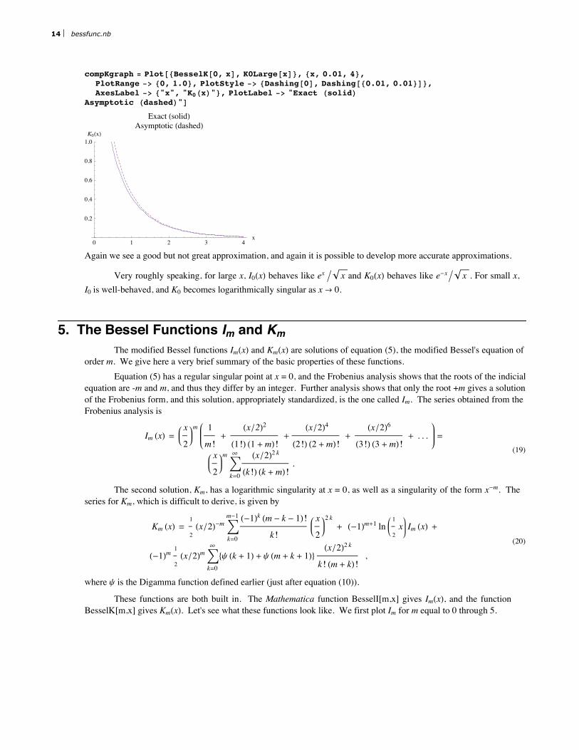
compKgraph = Plot@8BesselK@0, xD, K0Large@xD<, 8x, 0.01, 4<,PlotRange -> 80, 1.0<, PlotStyle -> 8Dashing@0D, Dashing@80.01, 0.01<D<,AxesLabel -> 8"x", "K0HxL"<, PlotLabel -> "Exact HsolidL

Asymptotic HdashedL"D

0 1 2 3 4x

0.2

0.4

0.6

0.8

1.0K0HxL

Exact HsolidLAsymptotic HdashedL

Again we see a good but not great approximation, and again it is possible to develop more accurate approximations.

Very roughly speaking, for large x, I0HxL behaves like ex ë x and K0HxL behaves like e-x ë x . For small x,I0 is well-behaved, and K0 becomes logarithmically singular as x Ø 0.

5. The Bessel Functions Im and KmThe modified Bessel functions ImHxL and KmHxL are solutions of equation (5), the modified Bessel's equation of

order m. We give here a very brief summary of the basic properties of these functions.Equation (5) has a regular singular point at x = 0, and the Frobenius analysis shows that the roots of the indicial

equation are -m and m, and thus they differ by an integer. Further analysis shows that only the root +m gives a solutionof the Frobenius form, and this solution, appropriately standardized, is the one called Im. The series obtained from theFrobenius analysis is

(19)

Im HxL =x

2

m 1

m !+

Hx ê2L2

H1 !L H1 + mL !+

Hx ê2L4

H2 !L H2 + mL !+

Hx ê2L6

H3 !L H3 + mL !+ . . . =

x

2

m‚k=0

¶ Hx ê2L2 k

Hk !L Hk + mL !.

The second solution, Km, has a logarithmic singularity at x = 0, as well as a singularity of the form x-m. Theseries for Km, which is difficult to derive, is given by

(20)

Km HxL =1

2Hx ê2L-m ‚

k=0

m-1 H-1Lk Hm - k - 1L !

k !

x

2

2 k+ H-1Lm+1 ln K

1

2x Im HxL +

H-1Lm1

2Hx ê2Lm‚

k=0

¶

8y Hk + 1L + y Hm + k + 1L<Hx ê2L2 k

k ! Hm + kL !,

where y is the Digamma function defined earlier (just after equation (10)).

These functions are both built in. The Mathematica function BesselI[m,x] gives ImHxL, and the functionBesselK[m,x] gives KmHxL. Let's see what these functions look like. We first plot Im for m equal to 0 through 5.

14 bessfunc.nb

graphIm = Plot@8BesselI@0, xD, BesselI@1, xD, BesselI@2, xD, BesselI@3, xD,BesselI@4, xD, BesselI@5, xD<, 8x, 0, 4<, AxesLabel -> 8"x", "Im"<D

1 2 3 4x

1

2

3

4

5

6

Im

We see the apparent exponential growth as before, but we also see that the higher order functions are slower to getstarted. The reason is that ImHxL has a factor xm, which means that the function and the first m - 1 derivatives vanish atx = 0.

Now let's take a look at a plot of Km for m = 0 through 5. We start with a slight offset in x to avoid the singular-ity at x = 0.graphKm = Plot@8BesselK@0, xD, BesselK@1, xD, BesselK@2, xD, BesselK@3, xD, BesselK@4, xD,

BesselK@5, xD<, 8x, 0.01, 4<, PlotRange -> 80, 5<, AxesLabel -> 8"x", "Km"<D

0 1 2 3 4x

1

2

3

4

5Km

We see the apparent exponential decay for large x as before, and the singularity at x = 0, which becomes stronger as mincreases.

There are simple asymptotic approximations for ImHxL and KmHxL for large x, given byILarge@m_, x_D := Exp@xD ê Sqrt@2 * p * xD

KLarge@m_, x_D := Exp@-xD * Sqrt@p ê H2 * xLD

By way of example, we compare the exact and asymptotic expressions for m = 3, beginning with Im.

bessfunc.nb 15

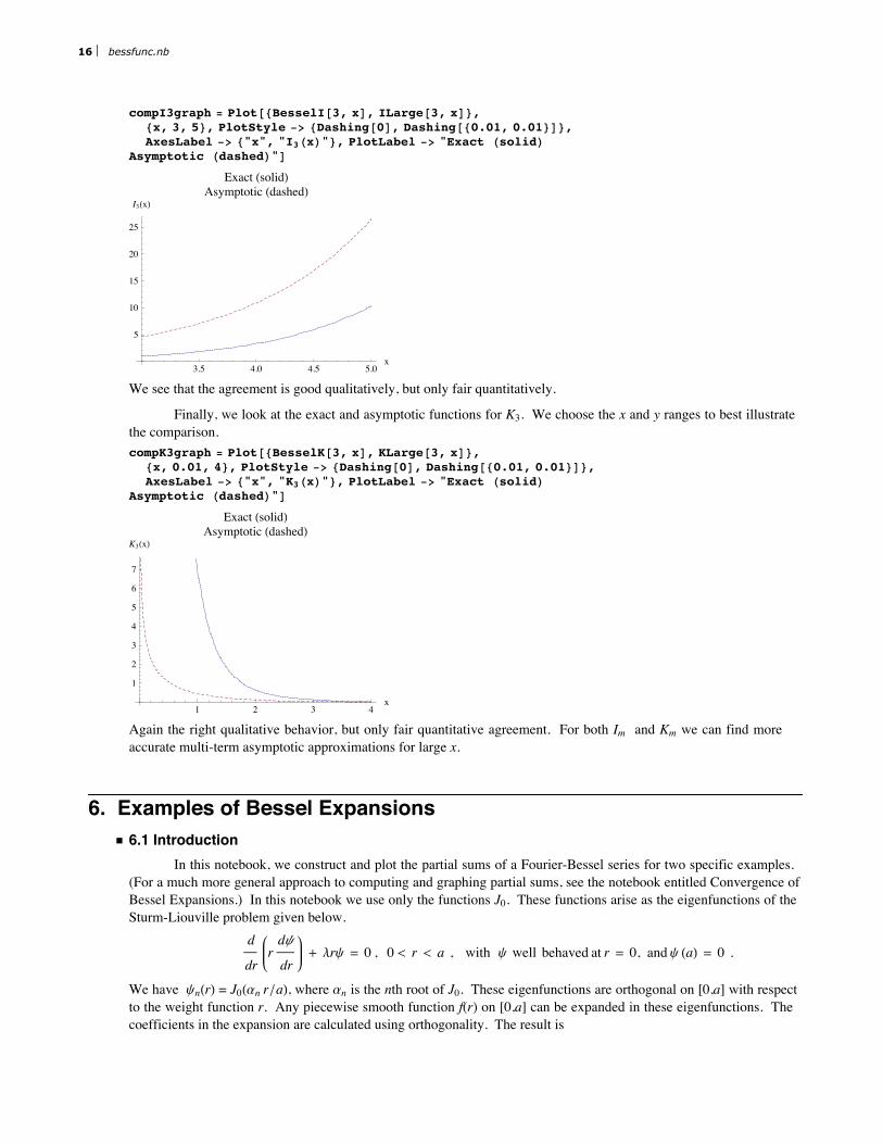
compI3graph = Plot@8BesselI@3, xD, ILarge@3, xD<,8x, 3, 5<, PlotStyle -> 8Dashing@0D, Dashing@80.01, 0.01<D<,AxesLabel -> 8"x", "I3HxL"<, PlotLabel -> "Exact HsolidL

Asymptotic HdashedL"D

3.5 4.0 4.5 5.0x

5

10

15

20

25

I3HxL

Exact HsolidLAsymptotic HdashedL

We see that the agreement is good qualitatively, but only fair quantitatively.

Finally, we look at the exact and asymptotic functions for K3. We choose the x and y ranges to best illustratethe comparison.compK3graph = Plot@8BesselK@3, xD, KLarge@3, xD<,

8x, 0.01, 4<, PlotStyle -> 8Dashing@0D, Dashing@80.01, 0.01<D<,AxesLabel -> 8"x", "K3HxL"<, PlotLabel -> "Exact HsolidL

Asymptotic HdashedL"D

1 2 3 4x

1

2

3

4

5

6

7

K3HxL

Exact HsolidLAsymptotic HdashedL

Again the right qualitative behavior, but only fair quantitative agreement. For both Im and Km we can find moreaccurate multi-term asymptotic approximations for large x.

6. Examples of Bessel Expansionsü 6.1 Introduction

In this notebook, we construct and plot the partial sums of a Fourier-Bessel series for two specific examples.(For a much more general approach to computing and graphing partial sums, see the notebook entitled Convergence ofBessel Expansions.) In this notebook we use only the functions J0. These functions arise as the eigenfunctions of theSturm-Liouville problem given below.

d

drr

dy

dr+ lry = 0 , 0 < r < a , with y well behaved at r = 0, and y HaL = 0 .

We have ynHrL = J0Han r êaL, where an is the nth root of J0. These eigenfunctions are orthogonal on [0,a] with respectto the weight function r. Any piecewise smooth function f(r) on [0,a] can be expanded in these eigenfunctions. Thecoefficients in the expansion are calculated using orthogonality. The result is

f(r) = ⁄n=1¶ Cn ynHrL , where Cn = Ÿ0

a f HrL yn HrL r „r

Ÿ0a8ynHrL<2 r „r

16 bessfunc.nb

f(r) = ⁄n=1¶ Cn ynHrL , where Cn = Ÿ0

a f HrL yn HrL r „r

Ÿ0a8ynHrL<2 r „r

ü 6.2 Example: f (r ) = a2- r2 on 0 £ r £ aWe now illustrate this theory by expanding the function

f@r_D := a2 - r2

We choose the value 3 for a:a = 3;

We find the first 21 zeros of J0 and assign them to the list named a. a = N@Table@BesselJZero@0, iD, 8i, 1, 21<DD

82.40483, 5.52008, 8.65373, 11.7915, 14.9309, 18.0711,21.2116, 24.3525, 27.4935, 30.6346, 33.7758, 36.9171, 40.0584,43.1998, 46.3412, 49.4826, 52.6241, 55.7655, 58.907, 62.0485, 65.19<

We define the eigenfunctions for Mathematica.y@r_, n_D := BesselJ@0, r * a@@nDD ê aD

We call the nth expansion coefficient coeff[[n]]. The theoretical expression is given above in equation (1). We defineexpressions for both the numerator and the denominator numerically in terms of the Mathematica function NIntegrate.We also obtain the coefficiencts below from an analytical expression derived in class. With more complicated func-tions f[r], numerical integration may be the only choice.num@n_D := NIntegrate@f@rD * y@r, nD * r, 8r, 0, a<D

den@n_D := NIntegrate@Hy@r, nDL^2 * r, 8r, 0, a<D

We calculate the first 21 coefficients, and assign them to a list named coeff.coeff = Module@8ans, c, n<, ans = 8<;

Do@Hc = num@nD ê den@nD; ans = Append@ans, cDL, 8n, 1, 21<D; ansD

89.9722, -1.258, 0.409288, -0.188918, 0.104726, -0.0649906, 0.0435408, -0.0308311,0.0227658, -0.0173713, 0.0136099, -0.0108969, 0.00888466, -0.00735654, 0.00617251,-0.00523902, 0.00449182, -0.0038857, 0.00338819, -0.00297548, 0.00262987<

In class, we also derived an analytical expression for these coefficients. Let's verify that we get the same resultthat way.

analcoeff@n_D := I8 a2M ë IHa@@nDDL3 BesselJ@1, a@@nDDDM;

analycoefflist =Module@8ans, c, n<, ans = 8<; Do@Hc = analcoeff@nD; ans = Append@ans, cDL, 8n, 1, 21<D; ansD;

We compare the two results by taking their difference.coeff - analycoefflist

9-8.88178 µ 10-15, -4.44089 µ 10-15, -2.38698 µ 10-14, 3.43059 µ 10-14,

7.4829 µ 10-14, 9.83241 µ 10-14, -1.88911 µ 10-13, -1.42483 µ 10-13, -1.31995 µ 10-13,-1.13333 µ 10-13, 2.02893 µ 10-14, -5.02948 µ 10-14, -5.39759 µ 10-14,-2.28427 µ 10-13, -9.65981 µ 10-15, 3.44247 µ 10-14, -3.7346 µ 10-14,-2.73956 µ 10-15, -8.99766 µ 10-14, -4.73168 µ 10-14, 1.19097 µ 10-14=

We get excellent agreement. Note that the fourth coefficient is only about 2% of the first coefficient, and the rest areeven smaller. This suggests rapid convergence, which we are about to verify with some graphs. This is not so surpris-ing given that the function being expanded satisfies the same zero boundary condition at the edge as the eigenfunctions.

Now we define the kth partial sum of our Fourier-Bessel series.fourbess@r_, k_D := Sum@coeff@@nDD * y@r, nD, 8n, 1, k<D

Finally, we define graph[k], which produces a graph of f[r] in blue and the kth partial sum of the Fourier-Bessel seriesin red. We use pltrange as a variable containing the plot range. We use SetOptions to set the value of the plottingoption Imagesize. We set it to 250, a good value for printing. For computer visualization, a value of 350 is better.

bessfunc.nb 17

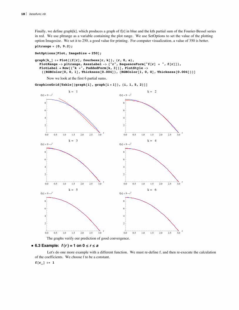
Finally, we define graph[k], which produces a graph of f[r] in blue and the kth partial sum of the Fourier-Bessel seriesin red. We use pltrange as a variable containing the plot range. We use SetOptions to set the value of the plottingoption Imagesize. We set it to 250, a good value for printing. For computer visualization, a value of 350 is better.pltrange = 80, 9.2<;

SetOptions@Plot, ImageSize Ø 250D;

graph@k_D := Plot@8f@rD, fourbess@r, kD<, 8r, 0, a<,PlotRange -> pltrange, AxesLabel -> 8"r", SequenceForm@"f@rD = ", f@rDD<,PlotLabel Ø Row@8"k =", PaddedForm@k, 3D<D, PlotStyle ->88RGBColor@0, 0, 1D, Thickness@0.004D<, 8RGBColor@1, 0, 0D, Thickness@0.004D<<D

Now we look at the first 6 partial sums.GraphicsGrid@Table@8graph@iD, graph@i + 1D<, 8i, 1, 5, 2<DD

0.0 0.5 1.0 1.5 2.0 2.5 3.0r

2

4

6

8

f@rD = 9- r2k = 1

0.0 0.5 1.0 1.5 2.0 2.5 3.0r

2

4

6

8

f@rD = 9- r2k = 2

0.0 0.5 1.0 1.5 2.0 2.5 3.0r

2

4

6

8

f@rD = 9- r2k = 3

0.0 0.5 1.0 1.5 2.0 2.5 3.0r

2

4

6

8

f@rD = 9- r2k = 4

0.0 0.5 1.0 1.5 2.0 2.5 3.0r

2

4

6

8

f@rD = 9- r2k = 5

0.0 0.5 1.0 1.5 2.0 2.5 3.0r

2

4

6

8

f@rD = 9- r2k = 6

The graphs verify our prediction of good convergence.

ü 6.3 Example: f (r ) = 1 on 0 £ r £ a Let's do one more example with a different function. We must re-define f, and then re-execute the calculation

of the coefficients. We choose f to be a constant.f@r_D := 1

18 bessfunc.nb

coeff = Module@8ans, c<, ans = 8<;Do@Hc = num@nD ê den@nD; ans = Append@ans, cDL, 8n, 1, 21<D; ansD

81.60197, -1.0648, 0.851399, -0.729645, 0.648524, -0.589543, 0.54418,-0.507894, 0.478012, -0.452851, 0.431284, -0.412531, 0.396028, -0.38136,0.368208, -0.35633, 0.345532, -0.335659, 0.326587, -0.318213, 0.310451<

Again we had an analytic expression for these coefficients in class, so again we use those in a consistency check.analcoeff@n_D := 2 ê Ha@@nDD BesselJ@1, a@@nDDDL

analycoefflist =Module@8ans, c<, ans = 8<; Do@Hc = analcoeff@nD; ans = Append@ans, cDL, 8n, 1, 21<D; ansD;

We take the difference to compare the numerical and analytical results.coeff - analycoefflist

9-1.55431 µ 10-15, -4.21885 µ 10-15, -5.973 µ 10-14, -6.68354 µ 10-14,

-7.21645 µ 10-14, 4.65183 µ 10-14, -9.76996 µ 10-14, 3.70814 µ 10-14,-8.27116 µ 10-15, -1.17129 µ 10-14, 2.88658 µ 10-15, -1.62648 µ 10-14,-3.7137 µ 10-14, 6.60583 µ 10-15, -8.82627 µ 10-15, 1.52101 µ 10-14, 1.94289 µ 10-15,-2.14828 µ 10-14, -7.77156 µ 10-16, 6.10623 µ 10-16, 2.04836 µ 10-14=

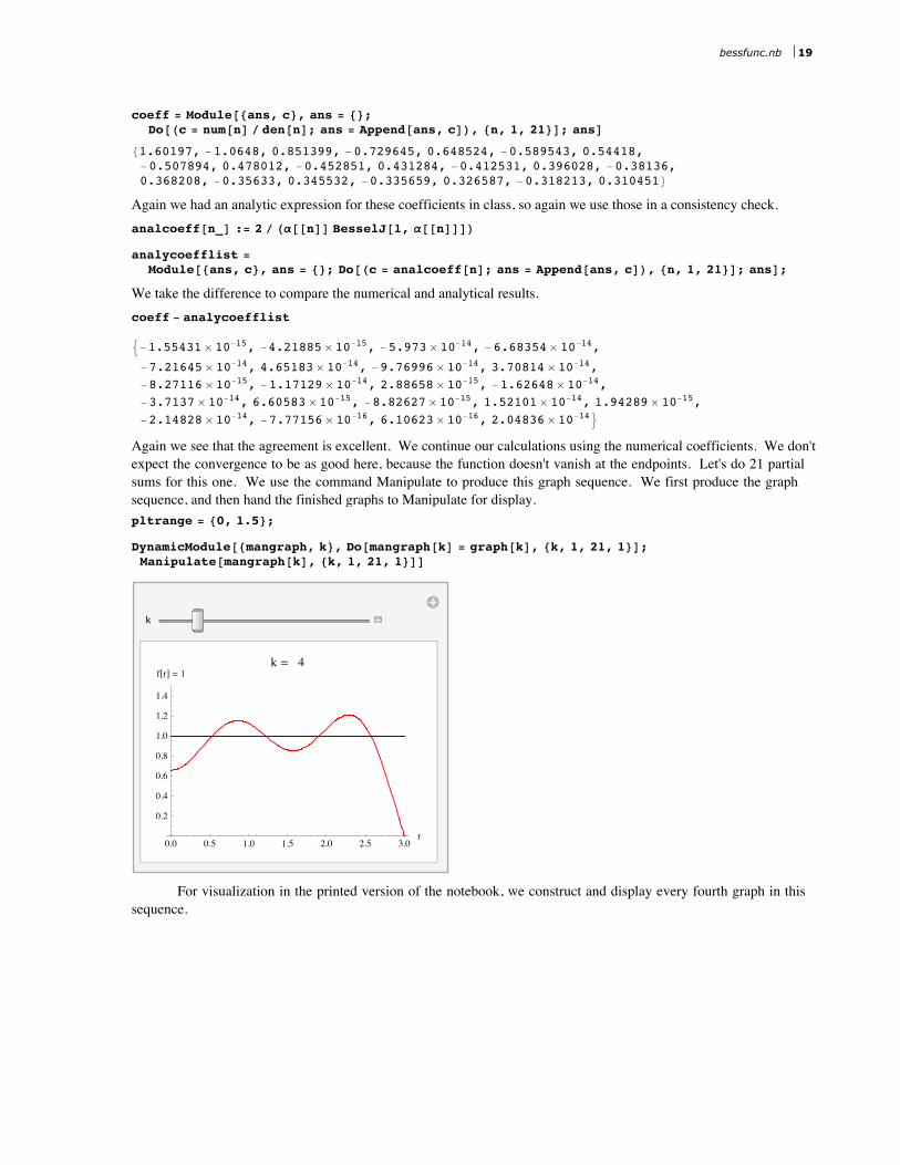
Again we see that the agreement is excellent. We continue our calculations using the numerical coefficients. We don'texpect the convergence to be as good here, because the function doesn't vanish at the endpoints. Let's do 21 partialsums for this one. We use the command Manipulate to produce this graph sequence. We first produce the graphsequence, and then hand the finished graphs to Manipulate for display. pltrange = 80, 1.5<;

DynamicModule@8mangraph, k<, Do@mangraph@kD = graph@kD, 8k, 1, 21, 1<D;Manipulate@mangraph@kD, 8k, 1, 21, 1<DD

k

0.0 0.5 1.0 1.5 2.0 2.5 3.0r

0.2

0.4

0.6

0.8

1.0

1.2

1.4

f@rD = 1k = 4

For visualization in the printed version of the notebook, we construct and display every fourth graph in thissequence.

bessfunc.nb 19

GraphicsGrid@Table@8graph@iD, graph@i + 4D<, 8i, 1, 17, 8<DD

0.0 0.5 1.0 1.5 2.0 2.5 3.0r

0.2

0.4

0.6

0.8

1.0

1.2

1.4

f@rD = 1k = 1

0.0 0.5 1.0 1.5 2.0 2.5 3.0r

0.2

0.4

0.6

0.8

1.0

1.2

1.4

f@rD = 1k = 5

0.0 0.5 1.0 1.5 2.0 2.5 3.0r

0.2

0.4

0.6

0.8

1.0

1.2

1.4

f@rD = 1k = 9

0.0 0.5 1.0 1.5 2.0 2.5 3.0r

0.2

0.4

0.6

0.8

1.0

1.2

1.4

f@rD = 1k = 13

0.0 0.5 1.0 1.5 2.0 2.5 3.0r

0.2

0.4

0.6

0.8

1.0

1.2

1.4

f@rD = 1k = 17

0.0 0.5 1.0 1.5 2.0 2.5 3.0r

0.2

0.4

0.6

0.8

1.0

1.2

1.4

f@rD = 1k = 21

The series is clearly converging, but the struggle is very reminiscent of the Fourier series for a square wave,complete with the Gibbs phenomenon. The resemblance is more than accidental. Remember that the Bessel functionsfor large argument (i.e., large n in the series) behave like damped trig functions, so the convergence issues are mathe-matically related to those of the Fourier series.

The above calculation has been very inefficient. In the sequence of 21 partial sums, we re-computed at eachstep all of the terms that appeared in the preceding graph, plus one new term. It would be far more efficient to save thenth partial sum, and then create the n+1st partial sum by computing only the new term and adding it to the nth partialsum. This is exactly what is done in the notebook Convergence of Bessel Expansions. In that notebook we will alsosee how to send the graph output to a Manipulate panel for convenience in visualization.

20 bessfunc.nb

7. Who Was Bessel?

Friedrich Wilhelm Bessel1784 - 1846

Bessel was born in Westphalia (Germany) in 1784. In spite of coming from a poor family, he entered businessat the age of 15 with an import-export firm. He was successful with the firm, but his natural intellect and curiosity ledhim through a sequence of studies including languages, geography, navigation, and astronomy and mathematics. Atthe age of 20 he published a paper on the orbit of Halley's Comet. The German astronomer Wilhelm Olbers was soimpressed with this work that he proposed Bessel as an assistant at the Lilienthal observatory. Thus Bessel was facedearly in his adult life with the choice between a business career of relative affluence or a career in science with a muchmore uncertain financial future. He chose the career in science.

Bessel's achievements are far too numerous to describe in detail, but here are a few brief examples. He studiedthe earth's size and shape, and in 1841 he deduced from his measurements that the ellipticity of the Earth is 1/299, aremarkably accurate result. He was a pioneer in precision measurement of stellar positions. His measurements ofstellar parallax led to some of the first accurate stellar distance determinations. For example, he determined that thestar 61 Cygni is about 10.3 light years from the earth. It is not an exaggeration to say that Bessel's work is one of thefoundations of our present knowledge of the scale of our universe.

Bessel's now famous equation arose in his studies of the mutual perturbations of planetary positions. He wasone of the first to make a serious effort on the notoriously difficult three-body problem in gravitational theory.

8. ReferencesThe literature on Bessel functions is enormous. There is a famous 800-page treatise on Bessel functions first

published in 1922 and still very useful:A Treatise on the Theory of Bessel Functions, by G.N. Watson, Cambridge University Press, 2nd edition,

1962.The single most useful practical reference for users of Bessel functions is

Handbook of Mathematical Functions, ed. M. Abramowitz and I. A. Stegun, National Bureau of Standards,1964.This reference has many useful formulas, graphs and tables for a wide variety of special functions. You can no longerbuy a hardbound copy for $6.50 as you could in 1964, but a relatively inexpensive paperback reprint is still available.A recent update of the above handbook is

NIST Handbook of Mathematical Functions, ed. Fran W.J. Olver,, Daniel W. Lozier, Ronald F. Bos=isvert,and Charles W. Clark, Cambridge University Press, 2010. The complete version of the NIST handbook is availableonline at http://dlmf.nist.gov/.

bessfunc.nb 21

This reference has many useful formulas, graphs and tables for a wide variety of special functions. You can no longerbuy a hardbound copy for $6.50 as you could in 1964, but a relatively inexpensive paperback reprint is still available.A recent update of the above handbook is

NIST Handbook of Mathematical Functions, ed. Fran W.J. Olver,, Daniel W. Lozier, Ronald F. Bos=isvert,and Charles W. Clark, Cambridge University Press, 2010. The complete version of the NIST handbook is availableonline at http://dlmf.nist.gov/.

The ultimate reference on special functions, including Bessel functions, is

Higher Transcendental Functions, Vol. I, II, and III, The Bateman Manuscript Project, ed. A. Erdelyi,W. Magnus, F. Oberhettinger, and F.C. Tricomi, McGraw-Hill, 1953.Volume II contains over 100 pages of formulas with Bessel functions.

Almost all texts on advanced calculus or mathematical methods for scientists and engineers have some usefulinformation on Bessel functions. There are hundreds of such books. Here are two by way of example -- the firstelementary and the second quite advanced:

Advanced Engineering Mathematics, E. Kreyszig, 7th and earlier editions, John Wiley.

Methods of Theoretical Physics, P.M. Morse and H. Feshbach, McGraw-Hill, 1953.

The historical information given in section 6 on Bessel came from the CD version of the Encyclopedia Brittan-ica, and from a web site at St. Andrews University devoted to the history of mathematics. The picture of Bessel alsocame from that web site. The web site is called the MacTutor History of Mathematics Archive, and its address is

http://www-groups.dcs.st-andrews.ac.uk/~history/ .

22 bessfunc.nb