Berth Allocation Planning Optimization in Container Terminals

Jim Dai ∗ Wuqin Lin † Rajeeva Moorthy ‡ Chung-Piaw Teo§

Abstract

We study the problem of allocating berth space for vessels in container terminals, whichis referred to as the berth allocation planning problem. We solve the static berth allocationplanning problem as a rectangle packing problem with arrival time constraints, using a localsearch algorithm that employs the concept of sequence pair to define the neighborhood struc-ture. We embed this approach in a real time scheduling system to address the berth allocationplanning problem in a dynamic environment. We address the issues of vessel allocation tothe terminal (thus affecting the overall berth utilization), choice of planning time window(how long to plan ahead in the dynamic environment), and the choice of objective used in theberthing algorithm (e.g., should we focus on minimizing vessels’ waiting time or maximizingberth utilization?). In a moderate load setting, extensive simulation results show that theproposed berthing system is able to allocate space to most of the calling vessels upon arrival,with the majority of them allocated the preferred berthing location. In a heavy load setting,we need to balance the concerns of throughput with acceptable waiting time experienced byvessels. We show that, surprisingly, these can be handled by deliberately delaying berthingof vessels in order to achieve higher throughput in the berthing system.

1 Introduction

Competition among container ports continues to increase as the differentiation of hub ports andfeeder ports progresses. Managers in many container terminals are trying to attract carriers byautomating handling equipment, providing and speeding up various services, and furnishing themost current information on the flow of containers. At the same time, however, they are tryingto reduce costs by utilizing resources efficiently, including human resources, berths, containeryards, quay cranes, and various yard equipment.

Containers come into the terminals via ships. The majority of the containers are 20 feet and40 feet in length. The quay cranes pick up the containers and load them into prime movers

∗School of Industrial and Systems Engineering, Georgia Institute of Technology, Atlanta, GA 30332, USA.

Email: dai@isye.gatech.edu†School of Industrial and Systems Engineering, Georgia Institute of Technology, Atlanta, GA 30332, USA.

Email: linwq@isye.gatech.edu‡Department of Decision Sciences, National University of Singapore, Singapore 119260. Email:

dscrlmk@nus.edu.sg§Department of Decision Sciences, National University of Singapore, Singapore 119260. Email: biz-

teocp@nus.edu.sg

1

(container trucks). The trucks then move them to the terminal yards. The yard cranes at theterminal yards then pick up the containers from the prime movers and stack them neatly in theyards according to a stacking pattern and schedule. Prime movers enter the terminals to pickup the containers for distribution to distriparks and customers. The procedure is reversed forcargo leaving the port. See Figure 1 for an example of a prime mover unloading containers froma vessel.

Figure 1: A prime mover unloading containers from a vessel

The problem studied in this paper is motivated by a berth allocation planning problem facedby a port operator. When planning berth usage, the berthing time and the exact position(i.e., wharf mark) of each vessel at the wharf, as well as various quay-side resources are usuallydetermined. Several variables must be considered, including the length-overall and (expected)arrival time of each vessel, the number of containers for discharging and loading on each vessel,and the storage location of outbound/inbound containers to be loaded onto/discharged from thecorresponding vessel. To minimize disruption and maximize efficiency, most of the customers(i.e., vessel owners) expect prompt berthing of their vessels upon arrival. This is particularlyimportant for vessels from priority customers (called priority vessels hereon), who may have beenguaranteed berth-on-arrival (i.e., within two hours of arrival) service in their contract with theterminal operator. On the other hand, the port operator is also measured by her ability toutilize available resources (berth space, cranes, prime-movers, etc.) in the most efficient manner,

2

with berth utilization,1 berthing delays faced by customers and terminal planning2 being primeconcerns.

We assume that the terminal is divided into several wharfs, which in turn are divided intoberths. Each wharf corresponds to a linear stretch of space in the terminal. Figure 2 shows thelayout of 3 terminals in Singapore. For instance, Keppel Terminal is divided into 5 wharfs, with5, 4, 3, 1 and 2 different berths in the 5 wharfs. Note that vessels can physically be berthedacross different berths, but they cannot be berthed across different wharfs.

Figure 2: Terminal layout in 3 terminals in Singapore

For each vessel calling at the terminal, the vessel turn-around time at the port can normallybe calculated by examining historical statistics (number of containers handled for the vessel, thecrane intensity allocated to the vessel, historical crane rate, etc.). Vessel owners usually requesta berthing time (called Berth-Time-Requested or BTR) in the terminal far in advance, and areusually allowed to revise the BTR when the vessel is close to calling at the terminal. Given a setof vessels calling at the terminal in a periodic schedule, our goal is to design a berthing systemto allocate berthing space to the vessels, to ensure that most vessels, if not all, can be berthedon-arrival, and that most of the vessels will be allocated berthing space close to their preferredlocations within the terminal. Note that the constraints in berthing space allocation give riseto non-convex domain, rendering the search for an optimal solution difficult. Furthermore, we

1This is the ratio of berth availability (hours of operations × total berth length) to berth occupancy (vessel

time at berth × length occupied). The utilization rate is affected by the number and types of vessels allocated to

the terminal. However, service performance (i.e., delays) will normally deteriorate with higher berth utilization,

since more vessels will be competing for the use of the terminal.2Containers to be unloaded from or loaded onto the vessels are normally stored at particular storage locations

within the yard. To minimize vessel turn-around time, the berthing location should ideally be selected close to

the storage location of the containers.

3

have to take into account the availability and accuracy of berthing time information, and mustbe able to determine an allocation dynamically over time.

In the berthing system, we define a scheduling window to be a time interval such that, at thebeginning of the interval, the arrival time and processing information on all relevant ships areknown. Here the relevant ships refer to all those ships that are currently at the terminal or willarrive at the terminal during the time interval. Of course, as time elapses, the scheduling windowrolls forward. An optimal packing within a scheduling window is a schedule of all relevant shipsthat optimizes a certain objective. Examples of objectives include maximizing berth utilizationwithin the window, maximizing throughput within the window, and minimizing berthing delayand space cost within the window.

Which objective should we use to obtain the packing within each scheduling window? Howoften should the packing schedules be produced? Do we update and change the vessel berthingplan in every scheduling window? How long should the scheduling window be? These decisionsaffect the size of the problem we need to solve in each scheduling window. The choice of theobjective function, coupled with the non-convex packing constraints, often lead to extremelydifficult combinatorial optimization problems. This leads us to the first issue related to theberth allocation planning problem:

Static Berth Allocation Problem:How do we design an efficient berth planning system to allocate berthing space to(say) 100 vessels in each berthing window?

Other than the above combinatorial complexity associated with berth planning, we also needto embed the plan in a dynamic berth planning system to allocate berthing space to vessels overtime. To do this, we need to address how the scheduling window is to be selected, and how oftento update the berthing plan for those vessels considered in earlier scheduling windows.

This leads us to the second issue related to the berth allocation planning problem:

Dynamic Berth Allocation Problem:How do we design a real time berth planning system to allocate berthing space tovessels which call at the terminal at regular intervals?

The berthing system is designed based on a rolling horizon framework. In a moderate load set-ting, we expect the berthing system to be able to accommodate most of the berthing constraintsand allocate space to vessels, minimizing waiting time experienced by vessels and optimizing theutilization of resources available in the terminal. In a heavy load setting, however, the trade-offis especially crucial, since the impact of inefficient resource utilization translates into large dropin throughput. To understand the difficulty in handling these problems, we use a simple exampleto illustrate the challenges faced in the dynamic berth allocation planning problem.

Example:Consider an example with three classes of vessels and a wharf with seven sections. Each class 1

4

vessel occupies 3 sections; each class 2 vessel occupies 4 sections; and each class 3 vessel occupies5 sections. Suppose the arrival rates of both class 1 and class 2 vessels are 1 vessel per 16 hours,and the arrival rate of type 3 vessels is 1 per 640 hours. The n-th class 1 vessel arrives at time16n − 5, class 2 at time 16(n − 1), and class 3 at time 640n. The processing times of the threeclasses of vessels are deterministic. They are 12 hours, 14 hours and 16 hours for class 1, class2, and class 3 vessels, respectively. Notice that, at most, two vessels can be processed eachtime. If we ignore the class 3 vessels, it is obvious that we can pack all the class 1 and class 2vessels immediately upon arrival. If we wish to minimize delays, the optimal packing is given byFigure 3.

Figure 3: Optimal Packing to minimize delays for class 1 and 2 vessels, when class 3 vessels areignored

However, with class 3 vessels being assigned to the terminal, the berthing system must nowaddress the trade-off between delays for vessels in the 3 different classes. How would a gooddynamic berth planning system handle the load situation presented by this example?

Case (a): Consider the situation where the most important objective in the scheduling windowis to maximize berth utilization within the scheduling window, and say the scheduling window ischosen to be W = 32 hours.

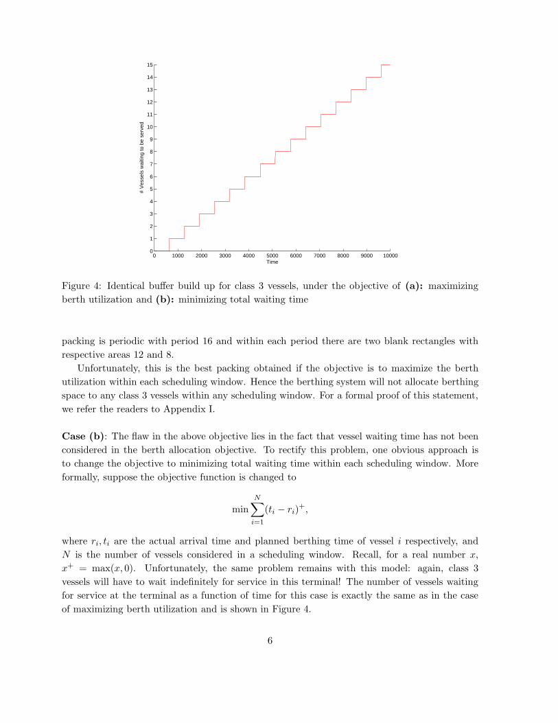
Figure 4 shows the number of vessels waiting for service over time. It reveals a major flaw inthe design of the above planning system: by focusing on berth utilization within the schedulingwindow, class 3 vessels will never have a chance to be served at all!

To understand why this is the case, note that the blank rectangles in Figure 3 are the capacity(measured by number of sections × time in hours) that can not be utilized. The space utilizationis determined by the total area of blank rectangles: the larger the blank area, the smaller theutilization. Denote U1(τ1, τ2) to be the unutilized capacity (blank area) between time τ1 and τ2

under the packing policy shown in Figure 3. For any τ ≥ 5, we have:

U1(τ, τ + 16) = 20. (1)

This is because under this packing policy during any period of 16 hours, sections 5-7 are idle for4 hours and sections 1-4 are idle for 2 hours. In fact, from Figure 3 one can observe that the

5

0 1000 2000 3000 4000 5000 6000 7000 8000 9000 100000

1

2

3

4

5

6

7

8

9

10

11

12

13

14

15

Time

# V

esse

ls w

aitin

g to

be

serv

ed

Figure 4: Identical buffer build up for class 3 vessels, under the objective of (a): maximizingberth utilization and (b): minimizing total waiting time

packing is periodic with period 16 and within each period there are two blank rectangles withrespective areas 12 and 8.

Unfortunately, this is the best packing obtained if the objective is to maximize the berthutilization within each scheduling window. Hence the berthing system will not allocate berthingspace to any class 3 vessels within any scheduling window. For a formal proof of this statement,we refer the readers to Appendix I.

Case (b): The flaw in the above objective lies in the fact that vessel waiting time has not beenconsidered in the berth allocation objective. To rectify this problem, one obvious approach isto change the objective to minimizing total waiting time within each scheduling window. Moreformally, suppose the objective function is changed to

minN∑

i=1

(ti − ri)+,

where ri, ti are the actual arrival time and planned berthing time of vessel i respectively, andN is the number of vessels considered in a scheduling window. Recall, for a real number x,x+ = max(x, 0). Unfortunately, the same problem remains with this model: again, class 3vessels will have to wait indefinitely for service in this terminal! The number of vessels waitingfor service at the terminal as a function of time for this case is exactly the same as in the caseof maximizing berth utilization and is shown in Figure 4.

6

This phenomenon can be explained by the fact that if class 3 vessels are berthed in anyscheduling window, it will induce delays on one class 1 vessel and one class 2 vessel. Hence ineach scheduling window, the class 3 vessels will be “sacrificed” and will have to wait for serviceindefinitely.

The above problem associated with dynamic berth allocation planning can be removed if weassign a higher priority status to vessels with larger length-overall (class 3 vessels) and assigna higher penalty for delaying vessels with higher priority, i.e., changing the objective to one ofminimizing weighted waiting time. Figure 5 shows the effect of using differentiated priorities toprevent buffer build-up. Note that class 3 vessels will be berthed upon arrival, due to the higherpriority status assigned. The queues built up can be cleared before the arrival of the next class3 vessels.

0 1000 2000 3000 4000 5000 6000 7000 8000 9000 100000

0.5

1

1.5

2

2.5

3

3.5

4

Time

# V

esse

ls w

aitin

g to

be

serv

ed

Figure 5: Buffer length over time when employing differentiated priority

This approach of assigning higher priority to vessels with larger length-overall, however, maylead to difficulties in other problem instances. For example, if the class 3 vessels occupy only 1section, with a port stay of 6 hours, then this weighted priority approach will assign low priorityto class 3 vessels. Class 1 and 2 vessels will be berthed immediately upon arrival, leaving onlygaps of 2 hours and 4 hours each between successive berthing (cf. Figure 3). In this case, again,class 3 vessels will not be berthed by the berth allocation planning system, leading to a reductionin terminal throughput. We need a different approach to guarantee near optimal throughput bythe terminal. In practice, the problem of assigning priority status to vessels is also complicatedby the fact that the priority status for some vessels is determined by the contractual agreementsigned between ports and customers, and cannot be arbitrarily assigned.

In the rest of this paper, we outline an approach to address the above issues associated with

7

the berth allocation planning problem. Our contributions can be summarized as follows:

• We solve the static berth allocation planning problem as a rectangle packing problem witharrival time constraints. The objective function chosen involves a combination of weightedwaiting time and allocated berthing space cost function. The optimization approach buildson the “sequence-pair” concept that has been used extensively in solving VLSI layout designproblems. While this method has been proven useful for addressing classical rectanglepacking problem to obtain tight packing, our rectangle packing problem is different as thekey concern here is to pack the vessel efficiently using the available berth space. Usingthe concepts of “virtual wharf marks”, we show how the sequence-pair approach can beaugmented to address the rectangle packing problem arising from the berth allocationplanning model.

• We extend the static berth allocation model to address the case where certain regions inthe time-space network cannot be used to pack arriving vessels. These forbidden regionscorrespond to instances where certain vessels have already been berthed and will leave theterminal some time later. In this case, the space allocated to these vessels cannot be usedto berth other arriving vessels. The ability to address these side constraints allows ourmodel to be embedded in a dynamic berth allocation planning model.

• In a heavy load setting, to ensure that throughput of the terminal will not be adverselyaffected due to the design of the berthing system, we propose a discrete maximum pressurepolicy to redistribute the load at the terminal at periodic intervals. We prove that thispolicy is throughput optimal even when processing times and inter-arrival times of vesselsare random. Interestingly, this policy ensures that vessels do not have to wait indefinitelyfor service, although the policy may deliberately insert delays on certain vessels, evenwhen the terminal has enough resources to berth the affected vessels on time. Withineach scheduling window, however, the static allocation planning problem will be solved toassign berthing space to the vessels. Hence this approach ensures that both the serviceperformance of the berthing system (BOA, preferred berthing space allocated, etc.) andterminal throughput performance are addressed by the berthing system.

• We conclude our study with an extensive simulation of the proposed approach, using aset of arrival patterns extracted and suitably modified from real data. As a side product,our simulation also illustrates the importance of the choice of scheduling windows, andthe trade-off between frequent revision to berthing plans and berthing performance. Notethat frequent revision of plans is undesirable from a port operation perspective, as frequentrevision has an unintended impact on personnel and resource schedules.

2 Literature Review

To the best of our knowledge, none of the papers in the literature address the dynamic berthplanning allocation problem proposed in this paper. Most of the existing papers focus mainly on

8

the static berth allocation problem, where the central issue is to obtain a good plan to pack thevessels waiting and arriving within the scheduling window. Brown et al. (1994) formulated aninteger-programming model for assigning one possible berthing location to a vessel consideringvarious practical constraints. However, they considered a berth as a collection of discrete berthinglocations, and their model is more apt for berthing vessels in a naval port, where berth shiftingof moored vessels is allowed. Lim (1998) addressed the berth planning problem by keeping theberthing time fixed while trying to decide the berthing locations. The berth was consideredto be a continuous space rather than a collection of discrete locations. He proposed a heuristicmethod for determining berthing locations of vessels by utilizing a graphical representation for theproblem. Chen and Hsieh (1999) proposed an alternative network-flow heuristic by consideringthe time-space network model. Tong, Lau, and Lim (1999) solved the ship berthing problemusing the Ants Colony Optimization approach, but they focused on minimizing the wharf lengthrequired while assuming the berthing time as given. In the Berth Allocation Planning System(BAPS) (and its later incarnation iBAPS) developed by the Resource Allocation and Scheduling(RAS) group of NUS, a two-stage strategy is adopted to solve the BAP problem. In the firststage, vessels are partitioned into sections of the port without specifying the exact berth location.The second stage determines specific berthing locations for vessels and packs the vessels withintheir assigned sections. See Loh (1996) and Chen (1998). Moon (2000), in an unpublishedthesis, formulated an integer linear program for the problem and solved using LINDO package.The computational time of LINDO increased rapidly when the number of vessels became higherthan 7 and the length of the planning horizon exceeded 72 hours. Some properties of the optimalsolution were investigated. Based on these properties, a heuristic algorithm for the berth planningproblem was suggested. The performance of the heuristic algorithm was compared with that ofthe optimization technique. The heuristic works well on many randomly generated instances,but performs badly in several cases when the penalty for delay is substantial.

The static berth planning problem is related to a variant of the two-dimensional rectanglepacking problem, where the objective is to place a set of rectangles in the plane without overlapso that a given cost function will be minimized. This problem arises frequently in VLSI designand resource-constrained project scheduling. Furthermore, in certain packing problems, the rec-tangles are allowed to rotate 90o. In these problems, the objectives are normally to minimize theheight or area used in the packing solution. Imahori et al. (2002), building on a long series ofwork by Murata et al. (1996), Tang et al. (2000), etc., propose a local search method for thisproblem, using an encoding scheme called sequence pair. Their approach is able to address therectangle packing problem with spatial cost function of the type g(maxi pi(xi),maxi qi(ti)), wherepi, qi are general cost functions and can be discontinuous or nonlinear, and g is nondecreasingin its parameters. Given a fixed sequence pair, Imahori et al. (2002) showed that the associ-ated optimization problem can be solved efficiently using a Dynamic Programming framework.Unfortunately, the general cost function considered in their paper cannot be readily extended toincorporate the objective function considered in this paper.

The berth allocation planning problem is also related to a class of multiple machines stochasticscheduling problems on jobs with release dates, where each job needs to be processed on multiple

9

processors at the same time, i.e., there is a given pre-specified dedicated subset of processorswhich are required to process the task simultaneously. This is known as the multiprocessor taskscheduling problem. Li, Cai, and Lee (1998) focused on the make-span objective and derivedseveral approximation bounds for a variant of the first-fit decreasing heuristic. However, theirmodel ignored the arrival time aspect of the ships and is not directly applicable to the berthingproblem in practice. In a follow-up paper, Guan et al. (2002) addressed the case with weightedcompletion time objective function. They developed a heuristic and performed worst case analysisunder the assumption that larger vessels have longer port stays. This assumption, while generallytrue, does not hold in all instances of container terminal berthing. Fishkin et al. (2001), usingsome sophisticated approximation techniques (combination of scaling, LP, and DP), derivedthe first polynomial time approximation scheme for this problem, for the minimum weightedcompletion time objective function. However, in the berth planning problem, since release timeof each job is given, a more appropriate objective function is to consider the weighted flow timeobjective function. Unfortunately, there are very few approximation results known for schedulingproblems with mean flow time objective function.

The closest literature to our line of work is arguably the series of papers by Imai, Nishimura,and Papadimitriou (2001, 2003). In the first paper, they proposed a planning model where vesselarrival time is modelled explicitly and they proposed a Lagrangian-based heuristic to solve theinteger programming model. Their model is a simplified version of our static berth allocationplanning problem, since they implicitly assume that each vessel occupies exactly one berth intheir model. The issue of re-planning is also not addressed in that paper. In the second paper,they proposed an integer programming model and a genetic algorithm for solving the static berthplanning model with differentiated priorities, but their model assumes deterministic data anddoes not take into consideration the arrival time information.

3 Static Berth Allocation Planning Problem

Given a scheduling window and information on the vessels that will be arriving within thewindow, we structured the associated berth planning problem as one of packing rectangles ina semi-infinite strip with general spatial cost structure. In this phase, the packing algorithmmust minimize the delays faced by vessels, with higher priority vessels receiving the promisedlevel of services. At the same time, the algorithm must also address the desirability, from a portoperator’s perspective, to berth the vessels on designated locations along the terminal and tominimize the movement and exchange of containers within the yards and between vessels.

The input to the problem are:

• Terminal specifics:

– W : Number of wharfs in the terminal,

– wi: Length of wharf i, i = 1, . . . ,W ,

– M : Number of berths in the terminal,

10

– Li: Length of berth i, i = 1, . . . ,M .

• Vessel specifics:

– N : Number of vessels that have arrived or will arrive within the scheduling window,

– ri: Arrival time of vessel i,

– li: Length-overall of vessel i,

– pi: Length of port stay upon berthing by vessel i.

In this paper, we assume that vessels can be moored at any berth available within the terminal.In real terminal berth allocation planning, we also have to take into account the issues of draftconstraints, equipment type availability along the berth, tidal information and crane availabil-ity; and we have to make sure that the berth allocation plan will not violate these additionalconsiderations. Furthermore, we note that although we take the vessel-specific parameters asgiven constants for each scheduling window, in reality, some of the parameters (such as arrivaltime within the scheduling window) may not be as forecast. In particular, the port stay time pi

depends on crane intensity (average number of cranes working on the vessel per hour) assignedto vessel i, and also on the number of containers to be loaded and discharged. This information,however, maybe not be accurate or available prior to the scheduling decision.

The decision variables to the berth planning problem are:

• xi: Berthing location for vessel i, measured with respect to the lower end of the vessel,

• ti: Planned berthing time for vessel i.

Given a berthing plan with prescribed decisions xi and ti, we can evaluate the quality of thedecision by two cost components:

• Location Cost: The quality of the berthing locations assigned is given by

N∑i=1

ci(xi),

where the space cost function ci is a step function in xi. Let dil be the penalty for berthingvessel i at berth l. Then,

ci(xi) = di,l if vessel i is berthed in berth l,

i.e.,

xi ≤l∑

k=1

Lk, xi >

l−1∑k=1

Lk.

Note that di,l indicates the desirability of berthing vessel i in berth l. This depends onwhere the loading containers are stored in the terminal and also on the destination of thedischarging containers.

11

• Delay Cost: The quality of the berthing times assigned is given by

N∑i=1

wi

(ti − ri − 2

)+

.

A vessel is considered “berthed-on-arrival” (BOA) if it can be berthed within two hours ofarrival (i.e., within ri and ri +2). This is the service level promised to some key customers.The value wi is a penalty factor attached to vessel i and indicates the “importance” ofberthing the vessel i on arrival (i.e., within a two-hour window). The vessels are normallydivided into several priority classes with different penalty factors.

The optimal packing problem in this phase can be formulated as the following Static BerthPlanning problem (SBP):

minN∑

i=1

(ci(xi)) +N∑

i=1

wi(ti − ri − 2)+ (2)

s.t. ti ≥ ri, ∀ i, (3)

xi + li ≤∑

i

Li, xi ≥ 0, ∀ i, (4)

xi is not berthed across different wharfs for all vessel i, (5)

ti + pi ≤ tj or tj + pj ≤ ti or xi + li ≤ xj or xj + lj ≤ xi ∀ i �= j. (6)

The last constraint models the condition that vessels i and j cannot occupy the same locationin the terminal at the same time. Note that this is a nonlinear optimization problem withnon-convex feasible region and is hence a difficult optimization problem.

3.1 Sequence Pair Concept

We first show that every berthing plan can be encoded by a pair of permutations of all vessels(H,V ). Consider the berthing plan of two vessels as shown in Figure 6.

Figure 6: The figure on the left shows the LEFT-UP view of vessel j, whereas the figure on theright shows the LEFT-DOWN view of vessel j; the views seen by vessel j are shaded regionsplus the parts blocked by vessel i.

12

The permutations H and V associated with the berthing plan are constructed with thefollowing properties:

• If vessel i is on the right of vessel j in H, then vessel j does not “see” vessel i on itsLEFT-UP view.

• Similarly, if vessel i is on the right of vessel j in V , then vessel j does not “see” vessel i onits LEFT-DOWN view.

It is clear that, given any berthing plan, we can construct a pair (H,V ) (need not be unique)satisfying the above properties. For any two vessels a and b, the ordering of a, b in H, V

essentially determines the relative placement of vessels in the packing. For the rest of the report,we write a <H b (and a <V b) if a is placed on the left of b in H (resp. in V ).

• If a <H b, a <V b, then a does not see b in LEFT-DOWN or LEFT-UP, i.e., vessel b is tothe right of vessel a. In other words, vessel b can only be berthed after vessel a leaves theterminal.

• If a <H b, b <V a, then a does not see b in LEFT-UP and b does not see a in the LEFT-DOWN view, i.e., vessel b is berthed below vessel a in the terminal.

For any H and V , either one of the above holds, i.e., either vessel a and vessel b do not overlapin time (one is to the right of the other) or do not overlap in space (one is on top of the other).

Note that every sequence pair (H,V ) corresponds to a class of berthing plans satisfyingthe above properties. The constraints imposed by the sequence pairs split into two classes:constraints of the type xi + li ≤ xj (in the space variables) or of the type ti +pi ≤ tj (in the timevariables). In this way, finding the optimal packing in this class, given a fixed sequence pair,decomposes into two subproblems: space and time (cf. Figure 7).

Given a fixed sequence pair, it will be ideal if the optimal berthing plan can be obtained in aLEFT-DOWN fashion, i.e., berthing each vessel at the earliest time and lowest possible positionavailable, subject to the sequence-pair condition. This method has various other advantages, asthe berthing plan for vessels can actually be constructed greedily in an iterative manner, allowingus to handle a host of other side constraints in real terminal berthing operations. Unfortunately,a LEFT-DOWN packing obtained with a fixed sequence pair may not always gives rise to theoptimal packing, due to the step-wise feature of the berthing space cost.

3.2 Time Cost Minimization With Fixed Sequence Pair

Given (H,V ), let GT be the directed graph associated with constraints involving the berthingtime variables ti. The time-cost problem can be formulated as:

minti

N∑i=1

wi(ti − ri − 2)+

subject to

13

Figure 7: Directed Graphs on the space and time variables arising from the Sequence Pair

• Berthing time must be as large as arrival time: ti ≥ ri for all vessels.

• ti + pi ≤ tj if (i, j) ∈ GT .

Letfi(ti) = wi(ti − ri − 2)+.

Since fi(·) is a non-decreasing function in ti, the optimal solution to the above is clearly to setti as small as possible, subject to satisfying all the constraints. This is the classical longest pathproblem in an acyclic digraph that can be solved easily using a simple dynamic-program. Onecan refer to Imahori et. al. (2003) for a dynamic programming based algorithm and Ahuja et.al. (1993) for a general discussion on longest path problems. In fact, each ti is selected to be thesmallest possible value satisfying the constraints and can be constructed in a greedy manner.

3.3 Space Cost Minimization With Fixed Sequence Pair

Given (H,V ), let GS be the directed graph associated with constraints involving the berthinglocation variables xi. The space-cost problem can be formulated as:

minxi

N∑i=1

N∑i=1

ci(xi)

subject to

14

• Berthing location cannot extend beyond the terminal: xi + li ≤ L, xi ≥ 0.

• Berthing location cannot cross wharf: xi + li ≤∑K

i=1 Li or xi ≥∑K

i=1 Li if the berth K

and berth K + 1 belong to different wharfs.

• xi + li ≤ xj if (i, j) ∈ GS .

Given arbitrary step function ci(·), solving the above problem is exceedingly difficult. In thecase when all li = 0 and GS corresponds to a Hamiltonian Path, the above is just the classicalnonlinear ordered set problem. In fact, berthing the vessel according to the lowest possibleposition satisfying the constraints may not always give rise to good packing. LEFT-DOWNpacking will not produce a good solution in terms of space cost.

To address this problem, we outlined a method where the space cost minimization problemcan be handled implicitly by extending the search space. We exploit the observation that thespace cost function are essentially step functions that depend on the number of berths in theterminal. Note that the number of berths in a terminal is relatively small (compared to thenumber of vessels). Furthermore, the space objective cost-function is constant within a berth.

In the special case where ci(·) is a constant function, the space cost minimization problem canbe solved efficiently as a longest path problem in GS , as in the previous case. In this instance,each vessel is berthed at the lowest possible position satisfying the precedence constraints andwharf-crossing constraints. For general ci(·), unfortunately, we need to consider all possibleberthing locations for vessel i in search of better berthing cost. This is the major bottleneck inthe search for an optimal solution in this problem.

For each berth l, we introduce a virtual wharf mark w(l) indicating a vessel with rw(l) =0, lw(l) = 0, pw(l) = 0, with additional constraint (lower-bound on berthing location)

xw(l) ≥l−1∑i=1

Li.

Note that the berthing plan on the left side of Figure 8 can be obtained from the sequence pair(12w34, 431w2) by berthing the vessels (real and virtual) using the left-down berthing approach.The introduction of the virtual wharf marks in the sequence pair and the added constraints onthe position of the wharf marks allow us to incorporate gaps into the berthing position of thevessels, and has virtually no impact on the berthing time. Note that it is not known, beforehand, how many wharf marks will be needed to prop up the vessels to the desired locationsin the terminal. But we note that for a sequence pair, with the right number of wharf marksdistributed appropriately, we can obtain the optimal packing by using the LEFT-DOWN packingstrategy. We record the observation in the following theorem.

Theorem 1. Suppose P∗ is the optimal berthing plan to the problem, minimizing the totalberthing time and space cost. Then there exists a set of virtual wharf marks {w1, . . . , wK}, forsome K, such that P∗ is equivalent to a berthing plan Q∗, involving all the vessels and virtualwharf marks, such that Q∗ is obtained from a corresponding LEFT-DOWN packing using somesequence pair H∗∗ and V ∗∗.

15

Figure 8: Berthing plan with virtual wharf mark as shown on the right. The sequence pairchanges from (1234, 4312) to (12w34, 431w2)

Proof: See Appendix II.

In general, finding the optimal number of wharf marks and their associations with the vesselsis extremely difficult. It also does not pay to find the optimal packing at every stage because thesequence pair may not correspond to the optimal solution. The main advantage of this approach isthat given any feasible packing, we can, through introduction of virtual wharf marks, encode thepacking as one obtainable from LEFT-DOWN from an associated sequence pair in an enlargedspace. This allows us to explore more complicated neighborhoods in the simulated annealingprocedure and its advantage will be evident in the next section.

3.4 Neighborhood Search Using Simulated Annealing

The approach outlined in the earlier section gives rise to an effective method to obtain a goodpacking, given a fixed sequence pair. We next use a simulated annealing algorithm to searchthrough the space of all possible (H,V ) sequence pairs. There are definitive advantages in usingsimulated annealing here, because now all the permutations of both the H and V sequence canbe explored in a systematic manner.

The critical aspect for getting good solutions is to define a sufficiently large neighborhoodthat can be explored efficiently. To this end, we use the following neighborhood structure:

(a) Single Swap: This is obtained by selecting two vessels and swapping them in the sequenceby interchanging their position. Single swap is defined when the swap operation is performed ineither H or V sequence.

(b) Double Swap: Double swap neighborhood is obtained by selecting two vessels and swappingthem in both H and V sequences.

16

(c) Single Shift: This neighborhood is obtained by selecting 2 vessels and sliding one vesselalong the sequence until the relative positions are changed; i.e., if i, j, . . . , k, l is a subsequence,a shift operation involving i and l could transform the subsequence to j, . . . , k, l, i. There aremany variants of this operation depending on whether vessel i (or l) is shifted to the left or rightof vessel l (or i). We define single shift as a shift operation along one of the sequences.

(d) Double Shift: This defines the neighborhood obtained by shifting along both H and V

sequences.Figure 9 shows examples of the above operations and their impact on the packing. The

above neighborhoods described are simple perturbations of the sequence pair, but they result inremarkably different packing when compared visually. On the other hand, it is pretty difficultto modify the sequence pair to obtain visually simple neighborhoods. For example, shifting arcsfrom space graph to time graph and vice versa between two vessels i and j without affecting theconstraints between the rest of the vessels and i and j is hard to obtain, though, visually, it maybe as simple as sliding vessel i from the top to the bottom of vessel j. Due to the non-linear spacecost, we observe that such neighborhoods would allow for shifting of vessels between differentberths and hence provide improvement in the solution. This motivated us to define the nextclass of neighborhood structure.

(e) Greedy Neighborhood: Given a sequence pair H and V and the associated packing P,we evaluate all possible locations that vessel i can take, with the rest of the vessels fixed in theirrespective positions. If there is a better location for the vessel, then we set the berth locationof i to its new location. Note that since the time is kept constant, it is easy to check whetherthere is an overlap along the space dimension. Once the vessel is placed in the new location, werepeat the procedure for the rest of the vessels, until no improvement is possible.

Figure 10 shows the packing and the corresponding sequence pair obtained from a simplegreedy neighbor.

The greedy neighborhood artificially modifies the position of the vessel along space. Hencewe may have cases where some vessels are placed on top of other vessels but none of the arcsin the space graph result in binding constraints. Fortunately, since the berthing space cost isconstant within every berth, we have the following conditions for the berthing location for eachvessel after the greedy modification: (i) the vessel i physically sits on top of another vessel, i.e.,xi = xj + lj where j is a vessel that overlaps with i along time; or (ii) xi =

∑k−1i=1 Li for some

berth k.In case (ii) above, we introduce a virtual wharf-mark to the sequence pair to create the

constraint that the vessel should be berthed above berth edge k.

Cooling schedule for simulated annealing: It is well known that the choice of the coolingschedule affects the results in simulated annealing since it is critical in the systems ability tomove away from local optima. For example, refer to Lin (1999). We evaluate the objective forthe packing as the sum of the time and space costs where time cost and space cost are definedas in sections 3.2 and 3.3. We did some tests using different cooling schedules and empiricallydetermined that the following schedule works well in our scenario:

17

Figure 9: Examples of swap and shift neighborhoods

18

Figure 10: Examples of greedy neighborhood

T0 =−Z0

ln 0.95,

Ti = Ti−1e−Ci.

The initial temperature T0 is determined based on the objective (Z0) of a greedily generatedinitial packing. The constant, 0.95, is an arbitrary choice and represents the probability ofmoving to inferior solutions during the first iteration of simulated annealing. After searching theneighborhood, we update the temperature Ti as shown. C is a constant and in our computation,we choose C = 0.99.

While searching at a specific temperature Ti, we denote the objective value at the beginningof the search as Z and the objective value for the current neighbor as Zj . The algorithm thenmoves to the new neighbor with the following probability:

• Probability of 1 if Zj < Z.

• Probability of e(Z−Zj)/Ti if Zj ≥ Z.

The algorithm is terminated when it reaches steady state (i.e., no further improvement canbe achieved in a few iterations) or when T = 0.

Implementation incorporating virtual wharf mark: The problem in adding virtual wharfmarks as additional vessels in the search space is that it increases the problem size and hencethe computation time. Here, we propose a cost-effective way of implementing the approach byemploying dynamic lower bounds.

Note that the vessels need to be propped after we employ the greedy neighborhood. Insteadof adding virtual wharf marks, the idea is to (dynamically) set lower bounds for the berthinglocation for those vessels that need to be propped by a virtual wharf mark in the packing. We

19

retain these lower bounds while exploring the neighborhood using operators (a)-(d), and changethe lower bounds only when operator (e) changes the packing and introduces new virtual wharfmarks.

The dynamic lower bounding technique described above is equivalent to adding a virtualwharf mark w to i (with w coming immediately after i in the H sequence, and w immediatelybefore i in the V sequence), and performing all neighborhood searches treating iw in H, andwi in V , as “virtual” vessel. Note that swapping or shifting iw with j in H, or swapping orshifting wi with j in V , has the same effect of swapping or shifting i with j in the original H

sequence, but maintaining a lower bound (determined by virtual wharf mark w) on vessel i inthe neighborhood.

3.5 Lower Bound For Static Berth Planning Problem

To evaluate the performance of the proposed approach, we need to compare the performanceagainst a suitable lower bound. To this end, we use tools from mathematical programming toobtain a lower bound to our berth planning problem.

The berth planning problem can be structured as a set packing problem with side constraints.Let Ci denote the set of allowed positions that vessel i can be berthed in the schedule. The setCi takes care of all the constraints in berthing positions (eg., no berthing across wharfs) andberthing times (eg., not earlier than arrival) of vessel i. The side constraints ensure that thevessels will not overlap.

Using standard Lagrangian relaxation approach, we can structure the problem as a set packingproblem to construct a lower bound to the problem. The bound is obtained by solving thefollowing:

maxπ(x,t)

min(xi,ti)∈Ci

N∑i=1

(ci(xi) + wifi(ti) +

∫ xi+li

xi

∫ ti+pi

ti

π(x, t)dxdt

)−

∫ L

0

∫ ∞

0π(x, t)dxdt.

The variables π(x, t) are the dual prices associated with the non-overlapping constraints (forthe position (x, t) in space). We use a version of subgradient algorithm, known as the volumealgorithm in the literature (cf. Barahona and Anbil (2000)), to solve the above problem.

To make the problem manageable so that the lower bound can be obtained within reasonabletime, the space-time network is discretized to moderate sizes using the following scaling technique:

• Let l = αL, where L is the length of the terminal, α is a scaling constant.

• For x in (0, L), define

u(x) =

{x if x

L(1 + Ll ) is an integer,

�(Ll + 1) x

L�l otherwise.

recall, for any real number x, �x� is the largest integer smaller than x.

20

Note that for the problem considered, and since all vessel lengths are integers, we do not expectto encounter instances where the vessel length x is such that x

L(1 + Ll ) is an integer. We may

thus assume all vessel lengths are scaled to multiples of l. This helps to reduce the size of theproblem considerably.

Proposition 1 ([10]). If∑

i∈S xi ≤ L, then∑

i∈S u(xi) ≤ L.

Note that the scaled problem will still provide us with a lower bound for the static berthplanning problem.

3.6 Computational Results

In this section, we compare the performance of the virtual wharf mark approach with that of thelower bound. We also show the difference in computational time taken to solve the problem. Wereport computational results on problem sizes including 30, 50, and 70 vessels. The instanceshave varying resource utilization (RU) levels. Average resource utilization is a measure of trafficload at the terminal and the max resource utilization measures the peak demand for berthingspace within the scheduling window. For each problem size, we compare the computationalperformances under two different scenarios:

• Congested Scenario: In this situation, all vessels available for packing arrive at time zero,thus creating intense competition for usage of the terminal. The instances in this scenarioare created with high average RU.

• Light Load Scenario: In this case, all vessels can be berthed immediately upon arrival andat the most preferred berth. We do this working backward, i.e., starting with a packing, wedevise cost parameters to the problem so that the packing is indeed the optimal solution.This is constructed by choosing appropriate values for vessel arrival time and preferredberthing locations. The average RU in these instances is typically lower and the max RUis always less than 1.

Figure 11 shows a typical plot of the convergence of the solution for simulated annealing andthe volume algorithm over consecutive iterations for a congested scenario. For sake of plots, onlythe final stages of simulated annealing iterations are plotted.

The computational performance for the experiments (averaged over 10 random instances) issummarized in Tables 1 and 2. Note that the proposed lower bound is understandably weak,since the Lagrangian relaxation model relaxes the non-overlapping constraints in the problem.The simulated annealing (SA) algorithm, on the other hand, is able to return a solution close to25%-36% of this lower bound (LB), depending on whether space cost is included in the modelor not. We believe that the quality of the solution obtained by the algorithm is much better.This is confirmed by the light load cases, where the simulated annealing algorithm is able toconsistently return close to optimal solution in all 10 random instances (< 0.33% vessels delayedand < 6.3% vessels placed in inferior locations).

21

Figure 11: Convergence of objective values for simulated annealing and lower bound for a con-gested scenario

# Vessels AvgRU %

MaxRU %

SpaceCost

Lowerbound(LB)

RunningTime(Sec)

HeuristicSolution(SA)

RunningTime(Sec)

(SA - LB)/ LB

30 60 250 No 613.8 52 794.3 15 0.32Yes 1645.6 54 2186.4 16 0.36

50 80 420 No 2119.6 69 2769.1 148 0.31Yes 2645.4 69 3468.9 155 0.33

70 75 580 No 5588.6 165 7260.3 643 0.31Yes 6503.1 165 8078.8 661 0.25

Table 1: Comparison with lower bound: congested scenario

# Vessels Avg RU % Max RU % Vessels Delayed Vessels in Inferior Berth30 25 60 0.33 % 2.67 %50 28 65 0.00 % 3.40 %70 37 82 0.29 % 6.29 %

Table 2: Performance of simulated annealing: light load scenario

22

4 Dynamic Berth Allocation Planning Model

In the dynamic berth allocation planning model, we have the additional challenge of rolling theplan forward every time we move forward one period. This raises an important question: Howdo we handle the situation when certain vessels are already berthed in the terminal? Note thatthe space allocated to these vessels cannot be used to berth other vessels.

We model these constraints as “forbidden zones” along the left edge of the berthing network.In the presence of infeasible regions in the packing area, to obtain one-to-one correspondencebetween the sequence pair and the packing, we use a variant of the lower bounding strategy,which can be viewed as an extension of the virtual wharf mark approach. In the earlier resultsby Murata, Fujiyoshi, and Kaneko (1998), infeasible regions were modeled as pre-placed vesselsand a greedy strategy was used to modify a packing to ensure that pre-placed vessels are restoredto their original locations. But with a complexity of O(N4) for instances with N vessels, it iscomputationally expensive. Herein we develop a strategy to specifically cater to the issue ofpacking during dynamic deployment. Figure 12 shows a typical scenario.

Figure 12: Handling pre-placed vessels

Along space, if a vessel is not supported below by another vessel (through the sequence-pairconditions), then we set an appropriate lower bound for the berthing location decision of thisvessel. Along time, if the vessel is adjacent to an infeasible region and there are no binding arcsin the time-graph, we can also set an appropriate lower bound to the berthing time decision ofthese vessels.

An initial packing is obtained using a greedy insertion strategy. The neighborhoods are thenexplored using the previous neighborhood structures, with the additional lower bound constraints

23

on berthing time and location decisions. We omit the details of the implementation here.

Revisions to berthing plan: The ability to build-in the latest arrival information and to reviseplans is definitely an advantage to the terminal operator in a dynamic setting; but frequentrevision of the berthing plan is not desirable from a resource planning perspective. This isdue to the fact that, based on the berthing plan, the port will normally have to plan the yardload and activate needed resources within the terminal to support loading/discharging activitiesfrom the vessels. In a container port, the following major resource-hogging events are affectedwhile servicing a particular vessel: Quay Cranes, Yard Cranes, Prime Movers, Operator-Crew,Container Movement, etc. Typically, the container and resource management in the yard is acomplex problem and is done beforehand based on the berth plan. Hence, any major deviationfrom the plan in a vessel’s location or service time, results in a major re-shuffle of crew and primemover allocations. It also results in re-deployment of cranes. Further, last minute changes tothe berthing plan and re-deployment of personnel and equipment lead to confusion. Hence it ispreferable that a proposed berth plan can be executed with minimal changes.

To ensure that the berthing plan will not be revised too frequently, the terminal operator canopt to freeze the berthing location decision made during earlier scheduling windows. Anotheralternative is to penalize deviation from an earlier plan by imposing a large penalty for changingthe berthing location or time for a vessel. We opt for the second strategy, where the space andtime cost function for vessel i is adjusted to

c′i(x) =

{0 if x = xi,

A otherwise,

f ′i(t) = A(t − ti)+,

where xi, ti are the earlier berthing decision, and A is a huge penalty term. The choice of c′i(·)and f ′

i(·) essentially forces vessel i to be berthed at the original berthing location and time.

5 Berth Planning With Throughput Consideration

The previous sections outlined a method to allocate berthing space to vessels in a dynamicenvironment. However, as shown in the earlier example, it does not preclude the possibilitythat certain classes of vessels will be delayed indefinitely and hence will not be berthed at allin the assigned terminal. This indirectly reduces the berth utilization and throughput of theterminal, which is a primary concern in berth planning. In this section, we propose a strategyto redistribute load within the terminal at periodic intervals, and we show that in this way, thethroughput of the terminal will be maximized.

To study the issue of throughput in the berth allocation planning problem, we use the frame-work of stochastic processing networks. We first discretize the berth space into integer units,indexed by k = 1, 2, . . . ,K. Each unit of the space is called a section. Each section can accom-modate one vessel each time, and each vessel occupies an integer number of consecutive sections

24

when it is moored. For ease of exposition, we group the vessels into categories or classes bythe number of sections they require3. All the vessels of the same class require the same numberof sections. The classes of vessels are indexed by i = 1, 2, . . . , I. Let K(i) be the number ofsections required by class i vessel. When no berth space is available, the vessel has to wait formooring. For each class of vessels, we create a (virtual) queue to buffer waiting and mooringvessels. This is a special class of the general stochastic processing networks advanced by Harrison(2000). An activity here accommodates a certain class of vessels and uses certain consecutivesections. Each activity is determined by the vessel class and the first section assigned to theactivity, and the activities are indexed by j = (i, k), i = 1, 2, . . . , I, k = 1, 2, . . . ,K − K(i) + 1.If activity j = (i, k) is taken, then the sections k, k + 1, . . . , k + K(i) − 1 are assigned to accom-modate (process) a class k vessel. Denote J to be the total number of activities. We define thecapacity consumption matrix A such that Akj = 1 if activity j requires section k and Akj = 0otherwise. Each activity takes care of one vessel each time. When several vessels are moored inthe berth, it is possible that several activities are active at the same time. An allocation is apossible set of active activities, which is defined by a binary J-vector a such that aj equals 1 ifactivity j is active in the allocation and 0 otherwise. We define the set of all possible allocationsA = {a : Aa ≤ e, aj = 0, 1 for each activity j}, where e is the K-dimensional vector of ones. Ascheduling policy dictates which allocation to use at any given time.

We use the following example to illustrate our model. Consider a wharf of length 200m. Wedivide it into 4 equal length sections (servers). If we assume all the vessel lengths are between75m and 125m, then the vessels are grouped into 2 classes. The vessels with length less than100m occupy two sections and belong to class 1; the vessels with length between 100m and 125mrequire three sections and belong to class 2. The stochastic processing network model for thisexample is depicted in Figure 13. Open rectangles represent buffers, circles represent sections,and activities are labeled on lines connecting buffers with sections. For terminology simplicity,the stochastic processing network model for the berth allocation problem is referred to as theberth allocation network.

Let Ei(t) be the cumulative number of class i vessels that have arrived by time t. Let Di(t)be the cumulative number of class i vessels that have departed by time t. For the stochasticprocessing network representation of the berth allocation problem, we assume the arrival rates(λi) are well defined. Namely, with probability one,

limt→∞

1tEi(t) = λi for each vessel class i.

The berth allocation network is said to be rate stable if for every initial configuration, withprobability one,

limt→∞

1tDi(t) = λi for each vessel class i.

In short, the berth allocation network is rate stable if the departure rate is equal to the arrival3In practice, these vessels may differ in preferred berth allocation. However, as we will focus on the throughput

attained in this section, we do not distinguish between these vessels.

25

Figure 13: A stochastic processing network model for berth allocation problem

rate for each vessel class. Obviously, if the offered load λi is too high, the berth allocationnetwork will not be rate stable no matter which scheduling policy is employed.

5.1 A Static Allocation Problem

Let ηj(n) (j = (i, k)) be the length of port stay upon berthing for the nth class i vessel mooredin sections k to k + K(i) − 1. The port stay length is allowed to be random. We assume thatthe processing rate µj is well defined. That is, with probability one,

limn→∞n−1

n∑�=1

ηj(�) = mj ,

where mj = 1/µj is the average length of port stay for vessels that are processed by activity j.Let Rij = µj if activity j takes care of class i vessels and Rij = 0 otherwise. Rij is the averagenumber of class i vessels that can be accommodated by a unit of activity j. We define theallocation a = 0 as idle allocation since all the servers (sections) are idle under this allocation.We characterize the stability condition by the following linear program:

min ρ (7)

s.t. Rx = λ, (8)

x =∑

a∈A\{0}aπa, (9)

∑a∈A\{0}

πa = ρ, (10)

πa ≥ 0 for each a ∈ A \ {0}. (11)

26

This linear program is closely related to LP (47)–(50) that was first introduced in Dai and Lin(2003) when preemption of jobs is not allowed. For each allocation a ∈ A\{0}, πa is interpretedas the long-run fraction of time that allocation a is employed. Then for each activity j, xj can beinterpreted as the long-run fraction of time that activity j is active. With this interpretation, theleft side of (8) is interpreted as the long-run net flow rate from the buffers. Equality (8) demandsthat exogenously inputs are processed to completion without other inventory being generated. ρ

is interpreted as the long-run fraction of time that at least one server is busy. In other words, ρ

is the utilization of the busiest server. This is different from the overall server utilization, whichaverages the utilization over all servers. It follows from Theorem 5 of Dai and Lin (2003) thatthe following theorem holds.

Theorem 2. If the berth allocation network is stabilizable, then the linear constraints (8)-(11)have a feasible solution with ρ ≤ 1.

5.2 Discrete Maximum Pressure Policies

We show that the converse of Theorem 2 is also true when processing times are bounded. That is,as long as ρ defined by LP (7)–(11) is strictly less than 1 and the processing times are bounded,then there is a scheduling policy under which the system will be rate stable.

We assume all the processing times are bounded by a constant U . For each class i, we defineZi(t) to be the number of class i vessels that have arrived at the terminal either waiting to beserved or being served at time t. We now define a family of policies, called discrete maximumpressure policies. They are adapted from Stolyar’s MaxWeight policy. See Andrew et al. (2001)and Stolyar (2002). The presentation here follows closely the definition of maximum pressurepolicies in Dai and Lin (2003). Define the pressure of a berth allocation network with buffer levelz under allocation a to be

p(a, z) =∑

j

aj

∑i

Rijzi = z · Ra.

The discrete maximum pressure policy with length L ≥ U is defined as follows.Discrete Maximum Pressure

• The time horizon is divided into cycles of length L.

• At the beginning of each cycle, an allocation with maximum pressure is selected, and eachsection is assigned to the vessel class given by the allocation until

(i) the corresponding buffer is empty or

(ii) it finishes a job and can not finish the next one within the cycle.

In both cases, the section is released and is ready to be assigned to any feasible activitythat can be finished within the cycle.

• One has flexibility to assign the released sections. We can allocate space from the releasedsection according to the objective outlined in the previous section, or we can do so suchthat the number of the remaining idle sections is minimized.

27

Theorem 3. Consider the berth allocation networks under any type of discrete maximum pres-sure policy with length L. If all the processing times are bounded by U , and the linear pro-gram (8)-(11) has a feasible solution with ρ ≤ ρ0 ≡ (L − U)/L, then the system is rate stable.

Variants of maximum pressure policies were first advanced by Tassiulas and Ephremides(1992) under different names for scheduling a multihop radio network. Their work was furtherstudied by various authors for systems in different applications; see Tassiulas and Ephremides(1992), Tassiulas (1995), McKeown et al. (1999), Dai and Prabhakar (2000), and Tassiulas andBhattacharya (2000).

To illustrate how the discrete maximum pressure policy works, consider the application ofthis policy in the example in Section 1. Note that the objective there is to maximize berthutilization within every scheduling window of 32 hours. It is easy to calculate ρ = 0.9 forthe example. We choose L = U/(1 − ρ) = 160 hours. Again, we only consider the activities(1, 1), (1, 5), (2, 1), (2, 4), (3, 1). Let allocation a1 = (0, 0, 1, 0, 0)′ be the allocation such that onlyactivity (2, 1) is active, allocation a2 = (0, 1, 1, 0, 0)′ be the allocation such that only activities(2, 1) and (1, 5) are active, allocation a3 = (0, 0, 0, 0, 1)′ be the allocation such that only activity(3, 1) is active, allocation a4 = (0, 0, 0, 1, 0)′ be the allocation such that only activity (2, 4) isactive, and allocation a5 = (1, 0, 0, 1, 0)′ be the allocation such that only activities (1, 1) and(2, 4) are active.

No class 3 vessel arrives in the first cycle (0, 160), and it follows the argument in Section 1that only activities (2, 1) and (1, 5) can be active by time L = 160 under our policy. Moreover,the allocation of the servers are the same as shown in Figure 3 during most of the cycle. However,some activities may be forced to be idle when they are close to the end of the cycle in order tomake all sections available at the beginning of the next cycle. In particular, activity (1, 5) staysidle from time 149 because another class 1 job will arrive at 153 and it can not be finished untiltime 167, while activity (2, 1) can finish the last job in the cycle at time 158. It is easy to seethat the buffer levels are Z1(160) = Z2(160) = 1 and Z3(160) = 0.

Then, at time t = 160, the beginning of the second cycle, allocations a2 and a5 are themaximum pressure allocations. Again without loss of generality, we choose allocation a2, andactivities (2, 1) and (1, 5) are employed. Similar to the first cycle, under maximum utilizationpacking scheme only activities (2, 1) and (1, 5) can be active and all except the first two vesselsare processed upon their arrival. At the end of the cycle, we have Z1(320) = Z2(320) = 1 andZ3(320) = 0. The third and fourth cycles will repeat the second cycle.

At time 640, the beginning of the fifth cycle, there is a class 3 arrival, so Z1(640) = Z2(640) =Z3(640) = 1. Allocations a2 and a5 are still the maximum pressure allocations as at the beginningof the previous 3 cycles. And under OUP packing, all vessels except the first two in the cycle willbe processed upon their arrival, so Z1(t) = Z2(t) = Z3(t) = 1 at time t = 800. The same goesfor cycle 6, 7, and 8, so at time t = 960, 1120, Z1(t) = Z2(t) = Z3(t) = 1, and at time t = 1280,Z1(t) = Z2(t) = 1 and Z3(t) = 2 because the second class 3 vessel arrives at time t = 1280, thebeginning of the ninth cycle.

Following the same argument, one can easily check that a2 and a5 are still the maximum

28

pressure allocations at the beginning of cycle 9 to cycle 11, and at time t = 1440, 1600, 1760,Z1(t) = Z2(t) = 1 and Z3(t) = 2. At time t = 1920, the beginning of the thirteenth cycle, thethird class 3 vessel arrives, so Z1(1920) = Z2(1920) = 1 and Z3(1920) = 3.

Now, the allocation a3 becomes the maximum pressure allocation. Activity (3, 1) will beemployed from time 1920. Note that buffer 3 has 3 vessels to be served and each requires 16hours processing time, so at time t = 1968, buffer 3 is empty and all the sections are released,and Z1(t) = Z2(t) = 4 and Z3(t) = 0 because there are 3 arrivals for each of class 1 and 2. UnderOUP packing, the sections are assigned to one class 1 and one class 2 vessel during the rest ofthe cycle from time 1968 to time 2080. During this time interval, there will be 7 arrivals for eachclass 1 and 2. On the other hand 9 class 1 and 8 class 2 vessels are served during the period, soZ1(2080) = 2, Z2(2080) = 3 and Z3(2080) = 0.

Therefore, at the beginning of the fourteenth cycle, all the class 3 vessels left while two class1 and three class 2 (including the one arriving at time 2080) vessels are waiting for mooring.The allocations a2 and a5 become the maximum pressure allocations again at time 2080. Itis easy to check that during the fourteenth cycle (2080, 2240), 10 vessels arrive for each class1 and 2 and 11 vessels of each class 1 and 2 are served during the cycle, so Z1(2240) = 1,Z2(2240) = 2 and Z3(2240) = 0. Similarly, we have at time 2400, the beginning of the sixteenthcycle, Z1(2400) = 1, Z2(2400) = 1 and Z3(2400) = 0. Since one class 3 vessel arrives at time2560, the beginning of the seventeenth cycle, Z1(2560) = 1, Z2(2560) = 1 and Z3(2560) = 1.Hence Z(2560) = Z(640). That is, the buffer size at the beginning of the seventeenth cycle isexactly the same as that of the fifth cycle. And due to the periodicity of the arrivals, one caneasily verify that the dynamics repeat every 1920 hours (12 cycles). Therefore, the system is ratestable.

5.3 Proof of Theorem 3

For a given buffer level z, define

M(z) = {argmaxa∈A

p(a, z)}.

M(z) is the set of allocations maximizing the network pressure given the buffer level z. For anyallocation a, we define a(z) such that

aj(z) =

{aj , zi(j) �= 0,0, zi(j) = 0,

where i(j) denotes the constituent buffer associated with activity j. We call a(z) the supportallocation of allocation a given the buffer level z. The buffer level of the constituent buffer ofany activity in a support allocation is positive.

Lemma 1. If a ∈ M(z), then a(z) ∈ M(z).

29

Proof.

p(a, z) =∑

j

ajRi(j),jzi(j) =∑

j,zi(j)>0

ajRi(j),jzi(j) =∑

j

aj(z)Ri(j),jzi(j) = p(a(z), z).

Lemma 1 says that for any buffer level z, we can always choose a support allocation withmaximum pressure. That is, there exists a maximum pressure allocation a∗ such that zi(j) > 0if a∗j > 0. Define M(z) to be the set of maximum pressure support allocations. Let I(z) be theset of buffers that have potential positive output flows under any maximum pressure supportallocation. Namely,

I(z) ={i(j) : aj > 0, a ∈ M(z)

}.

Notice that zi > 0 for any i ∈ I(z) because any i ∈ I(z) is a constituent buffer of some activityin a support allocation.

Lemma 2. For any allocations a1, a2, if a1 ≥ a2 then p(a1, z) ≥ p(a2, z) for any z ≥ 0. Herea1 ≥ a2 means a1

j ≥ a2j for any j.

Proof. Notice that Ri(j),j ≥ 0 for all j. Therefore,

p(a1, z) =∑

j

a1jRi(j),jzi(j) ≥

∑j

a2jRi(j),jzi(j) = p(a2, z).

Recall that Zi(t) counts the number of class i vessels at the terminal at time t. We use Z(t)to denote the corresponding vector. For each allocation a, we use Ta(t) to denote the cumulativeamount of time that allocation a has been used by time t, and T (t) to denote the correspondingvector Ta(t), a ∈ A. In the following lemma and the rest of this section, fluid limits of the berthallocation network are used. They are obtained as limits of T and Z under a law-of-large-numberstype scaling. Equations that are satisfied by fluid limits are said to be fluid model equations.These equations define a fluid model of the corresponding berth allocation network. Fluid limitsand fluid model are now quite standard objects in the stochastic processing network literature;see, for example, Section 5.3 of Dai and Lin (2003). In the following, (Z, T ) denotes a fluid limitof the berth allocation network operating under a discrete maximum pressure policy.

Lemma 3. Under discrete maximum pressure policy, each fluid limit (Z, T ) satisfies the fluidmodel equation: ∑

a∈M(Z(t))

˙Ta(t) ≥ (L − U)/L, t ≥ 0. (12)

30

Proof. Let (Z, T ) be a fluid limit. Let allocation a ∈ A\M(Z(t)) be any non-maximum-pressureallocation, and allocation a∗ ∈ M(Z(t)) be any maximum pressure support allocation. Thenp(a, Z(t)) < p(a∗, Z(t)). On the other hand, we know Zi(t) > 0 for any i ∈ I(Z(t)). By thecontinuity of Z(·), there exist ε > 0 and δ > 0 such that for each τ ∈ [t− ε, t+ ε] and i ∈ I(Z(t)),

p(a, Z(τ)) + δ ≤ p(a∗, Z(τ)) and Zi(τ) ≥ δ.

Thus, when n is sufficiently large, p(a,Z(nτ)) + nδ/2 ≤ p(a∗, Z(nτ)) and Zi(nτ) ≥ nδ/2 foreach a∗ ∈ M(Z(t)), each i ∈ I(Z(t)) and each τ ∈ [t − ε, t + ε]. Choosing n > 2J/δ, then foreach τ ∈ [n(t − ε), n(t + ε)] we have

p(a∗, Z(τ)) − p(a,Z(τ)) ≥ J, for each a∗ ∈ M(Z(t)) (13)

Zi(τ) ≥ J for each i ∈ I(Z(t)). (14)

Condition (14) implies that any allocation a∗ ∈ M(Z(t)) is a feasible allocation at the beginningof any cycle in [n(t−ε), n(t+ε)] because a∗ only processes jobs from buffers in I(Z(t)). Following(13) and the definition of the discrete maximum pressure policy, the allocation a will not beselected at the beginning of any cycle during time interval [n(t − ε), n(t + ε)].

Then we claim if the non-maximum-pressure allocation a is not employed at the beginning ofa cycle in the interval [n(t− ε), n(t+ ε)], then it will not be employed at the first L−U time unitsin that cycle. Let t0 be the beginning of any cycle in [n(t− ε), n(t+ ε)], and suppose allocation a

is employed at time t0. From the previous argument, a must be a maximum pressure allocation.That is, a ∈ M(Z(t)). From Lemma 1, the corresponding support allocation must be maximumpressure support allocation, or ¯a(Z(t)) ∈ M(Z(t)). Then i(j) ∈ I(Z(t)) for any j ∈ ¯a(Z(t))by the definition of I(Z(t)). (For an allocation a, we adopt the convention that j ∈ a if andonly if aj > 0.) Consequently, any activity j ∈ ¯a(Z(t)) will be employed during [t0, t0 + L − U ]because j ∈ a and Zi(j)(τ) > J for τ ∈ [n(t − ε), n(t + ε)]. If a is employed at any time during[t0, t0 + L − U ], then a ≥ ¯a(Z(t)). And hence p(a, Z(t)) ≥ p(¯a(Z(t)), Z(t)) = p(a, Z(t)), whichimplies a is a maximum pressure allocation given Z(t). We have a contradiction with the fact thata is not a maximum pressure allocation. Therefore, only the allocations in M can be deployedin the first (L − U) time period of any cycle in the time interval [n(t − ε), n(t + ε)]. That is,∑

a∈MTa(t0 + L) − Ta(t0) ≥ (L − U). (15)

There are more than (2nε − 2L)/L whole cycles during the interval [n(t − ε), n(t + ε)]. Thisimplies ∑

a∈MTa(n(t + ε)) − Ta(n(t − ε)) ≥ ((2nε − 2L)/L)(L − U). (16)

So∑

a∈M Ta(t + ε) − Ta(t − ε) ≥ 2ε(L − U)/L, and hence∑

a∈M˙Ta(t) ≥ (L − U)/L.

31

Lemma 4. Under a discrete maximum pressure policy with length L,∑a∈A

˙Ta(t)p(a, Z(t)) ≥ ρ0p(a′, Z(t)) for all a′ ∈ A, (17)

where, as before, ρ0 = (L − U)/L.

Proof. ∑a∈A

˙Ta(t)p(a, Z(t)) ≥∑

a∈M(Z(t))

˙Ta(t)p(a, Z(t)) (18)

≥∑

a∈M(Z(t))

˙Ta(t)p(a′, Z(t)) (19)

≥ ρ0p(a′, Z(t)). (20)

For any allocation a ∈ A, we define the potential net flow rate out of buffer i ∈ I under theallocation as

vi(a) =∑

j

Rijaj − λi.

Let vi(t) = − ˙Zi(t) be the actual net flow rate out of buffer i ∈ I at time t. It follows that

vi(t) =∑

j

Rij˙Tj(t) − λi.

Lemma 5. Under a discrete maximum pressure policy with length L,

v(t) · Z(t) ≥ v(ρ0a) · Z(t) for all a ∈ A. (21)

Proof. First, notice that

v(t) · Z(t) =∑

i

∑j

Rij˙Tj(t)Zi(t) − λ · Z(t)

=∑a′∈A

˙Ta(t)∑

i

∑j

Rija′jZi(t) − λ · Z(t)

=∑a′∈A

˙Ta(t)p(a′, Z(t)) − λ · Z(t),

and

v(a) · Z(t) =∑

i

∑j

RijajZi(t) − λ · Z(t)

= p(a, Z(t)) − λ · Z(t).

32

It follows that

v(t)Z(t) − v(ρ0a)Z(t) =∑a′∈A

˙Ta(t)p(a′, Z(t)) − p(ρ0a, Z(t)) (22)

=∑a′∈A

˙Tap(a′, Z(t)) − ρ0p(a, Z(t)) (23)

≥ 0 (24)

Proof of Theorem 3. Following Theorem 3 of Dai and Lin (2003), it is enough to prove that foreach fluid limit (Z, T ), Z(t) = 0 for t ≥ 0.

Let (ρ, x, π) be a solution to (8)-(11), and (Z, T ) be a fluid limit. Then∑

a∈A\{0}(πa/ρ) = 1,and ∑

a∈A\{0}(πa/ρ)v(ρa) =

∑a∈A\{0}

Rx − λ = 0.

Because ρ0 ≥ ρ, v(t) · Z(t) ≥ v(ρ0a) · Z(t) ≥ v(ρa) · Z(t) for all a ∈ A. Then

v(t) · Z(t) ≥∑

a∈A\{0}(πa/ρ)v(ρa) · Z(t) = 0.

Consider the following quadratic Lyapunov function:

f(t) =∑

i

Z2i (t). (25)

Assume that t is a time at which (Z, T ) is differential and f(t) > 0.

f(t) = 2 ˙Z(t) · Z(t) = −2v(t) · Z(t) ≤ 0. (26)

Since Z(0) = 0, it follows that Z(t) = 0 for all t ≥ 0.

6 Simulation Results

There are many variables that affect the dynamic deployment scenario and the impact can onlybe studied by using a simulation model.

Arrival pattern: We generate arrival to the terminal using an arrival pattern representative ofa typical port (cf. Figure 14). There are 48 vessels scheduled to call at the terminal on a weeklybasis and the figure shows the expected time of call during a week for each vessel. There areseveral other vessels shown below the chart, and these correspond to vessels which do not callweekly at the terminal, but may call every 10 days.

Design of experiment: The following describes the events regarding vessel arrival times andthe subsequent planning and execution that is done prior to berthing a vessel. The experimentalsetup for the simulations also follows these events.

33

Figure 14: Template for the simulation

34

• The vessels follow a cyclic arrival with a period of 7 (regular calls) or 10 (irregular calls)days.

• The arrival time according to the template is the Initial Berth Time Requested (IBTR)by the vessels. The actual arrival time is stochastically distributed with the Initial BerthTime Requested as the mean arrival time and a large variance.

• In practice, the vessel captain is allowed to update the arrival time twice before actuallyreaching the port. Firstly, a few days before arrival (in simulation, we assume 48 hours),the captain updates the port with an Updated Berth Time Requested (UBTR). This is amore accurate estimate of the actual arrival time and in the simulation, we obtain thearrival time from a stochastic distribution with the Updated Berth Time Requested as themean and a smaller variance. Furthermore, the exact time at which the different vesselsupdate this information will be different. In the simulation, we randomly generate theexact time that every vessel reports the Updated Berth Time Requested.

• At another time fence, very close to the current time, usually in the order of 1-2 shifts,the exact arrival time is reported. In the case of our simulation, we assume that vesselswill update their exact arrival time when the Updated Berth Time Requested is around 16hours away from current time. As before, we randomly generate the time when each vesselreports the exact arrival time.

• The experiments are performed for 15 weeks and the results are reported only for the first14 weeks to eliminate boundary effects.

• The vessels are randomly partitioned into seven priority classes, and the preferred berthlocation is generated according to the berthing location within the template.

• Typically, the berth locations are fixed (or minimum changes made) for the vessels setto arrive in the nearest shifts. This is done to prevent last minute resource re-allocation,which may lead to inefficient resource management. Based on this, we define a notionof steadiness. Steadiness is measured based on changes in the plan and the executionwithin the next 2 shifts (16 hrs) from the current time. In the simulation, to ensure 100%steadiness, we will also impose upper and lower bound constraints on the berthing locationof the vessels.

• Since the exact arrival time of the vessel is not known, and due to the fact that a vessel mayupdate the exact arrival information at any time, we measure steadiness based only on thechanges in vessel location. In the simulation, we allow changes in the planned and realizedberthing times. But we ensure that the variation is kept to a minimum by restricting theearliest and latest update time.

The results from Section 5 show that the port operator should definitely load the vessels inthe terminal so that ρ < 1 in the LP defined by (8) - (11). In this case, to ensure rate stability,

35

the port should set a planning window L and apply the discrete maximum pressure policy toredistribute the load in the terminal every L period. This, however, is costly since it requires theport to clear/delay all vessels prior to the beginning of each planning cycle. In reality, however,the load in the terminal should be selected in such a way that no vessel will experience substantialdelays while waiting for berthing, i.e., the heavy traffic situation should ideally be avoided. In amoderate load scenario, by looking ahead of the scheduling window, we hope to be able to planfor future load in an adequate manner so that current decisions will not produce undesirableeffects in the future. We will avoid the costly exercise of rebalancing the load in the terminal byusing the discrete maximum pressure policy.

We specifically run the following test scenarios and compare the performance of the dynamicberth allocation planning model in a rolling horizon setting. For comparison, we generate theInitial Berth Time Requested and the Updated Berth Time Requested beforehand and run thefollowing experiments. There are some managerial issues that are interesting to study in theberth planning problem. The developed simulation package allows us to study the impact ofthese on the overall performance of the system. For instance, we test the effect of the planningtime window, i.e., how far to look ahead in the scheduling window at each period. There is atrade-off between myopic planning (small time window) and inaccuracy in data (long time win-dow). We also test the trade-off between the objective of attaining high BOA for vessels, andthe desire to minimize replanning of activities.

Experiment A: Forecast is accurate.In this experiment, the actual arrival time of vessels follows the data as given, i.e., the IBTR

corresponds to the actual arrival time. This test represents the current arrival scenario andprovides a bench mark for the performance of the proposed system. Ideally, if we use the 48vessels scenario in Figure 14, and if the arrival time is accurately reflected, we expect all vessels toattain BOA status and to be berthed at their preferred location. Table 3 shows the results from arun of the simulation package, with a planning time window of 48 hours. Furthermore, berthingplan for vessels due to arrive over the next 16 hours (where arrival time is known exactly) isfrozen.

96% out of 672 vessels served in the 14 week simulation environment received BOA treatment,and close to 85% were berthed at their designated preferred berths.

The above results indicate that the proposed dynamic berth allocation planning model per-forms extremely well in this environment.

Experiment B: Template-based data with uncertainty in arrival time.In this setting, we assume that the actual arrival time has variance 30 and 10 with respect

to IBTR and UBTR respectively. We examine the impact of the planning window on the per-formance of the algorithm. Again, the berthing plan for vessels due to arrive over the next 16hours (where arrival time is known exactly) in each planning time window will be frozen.

We summarize the simulation results in Table 4. Interestingly, the results show the advantage

36

Class # of vessels served % BOA Average Delays (Hr) % Allocated Preferred Berth0 126 90 0.38 791 56 75 0.50 502 56 100 0.00 1003 84 100 0.00 824 70 100 0.00 975 210 100 0.00 876 56 100 0.00 967 14 100 0.00 93

Table 3: Simulation results obtained for Experiment A

of incorporating the longer planning time window of 72 hours over the shorter planning timewindow of 16 hours. Advance information on vessel arrival time, despite the uncertainty in theinformation, is still beneficial for the terminal in terms of berth planning. This is mainly becausethe plan for the first 16 hours will be frozen, and hence advance arrival information beyond thefirst 16 hours helps the terminal to obtain better berthing plan.

Windows % BOA Average Delays (hr) % Allocated Preferred Berth16 88 0.81 7024 89 0.53 7548 90 0.72 7872 93 0.33 76

Table 4: Simulation results obtained for Experiment B

Experiment C: Effect of freezing berthing plan. In this setting, we compare the perfor-mance of the model under the same setting as experiment B, except that the port will replanand possibly change berthing positions every time there is an update on vessel arrival data, i.e.,we do not freeze the berthing plan in every planning window.

Windows % BOA Average Delay (Hr) % Allocated Preferred Berth % Steadiness16 94 0.25 78 2324 94 0.23 75 2948 94 0.26 73 3172 93 0.29 75 38

Table 5: Simulation results obtained for Experiment C

In this case, the ability to replan allows the model to achieve better performance in terms ofBOA and preferred berth allocation statistics. Furthermore, the advantage of a longer planning

37

time window is no longer apparent. By planning using only the accurate arrival information(within first 16 hours), and with the capability to update the berthing plan every hour, the ter-minal can achieve an equivalent performance to the case when longer planning time windows areused. However, this comes at a price of frequent berthing plan revisions, which is undesirable.In the table, steadiness is a measure of the number of vessels that remain at the same locationwithin the 16 hour period. In Experiment B, steadiness is 100%.

Experiment D: Effect of differentiated priorities. In this experiment, we study the effectof differentiated priorities on the performance of the system, using a planning time window of 48hours. We compare average BOA and preferred berth allocation between the current system (withdifferentiated priorities), and the case when all vessels are accorded high or low priority status.Note that in the equal-high scenario, the overriding concern is to berth all vessels on arrival. Inthe equal-low scenario, the focus is on maximizing the benefits of preferred berth allocation. Asin experiment C, we do not freeze the berthing plan in this case. Table 6 summarizes the resultsobserved.

Priority % BOA Average Delay (Hr) % Allocated Preferred Berth % SteadinessDifferentiated 94 0.26 73 31Equal-High 97 0.14 67 30Equal-Low 90 0.58 86 46

Table 6: Simulation results obtained for Experiment D

The results indicate a good balance between the desire to obtain high BOA with a highpercentage allocated to preferred berth.

Experiment E: Irregular arrivals. Here, we repeat the experiment set up in A, but witha loading profile according to Figure 14, including the vessels with a cycle time of 10 days.Table 7 shows the results obtained with the added classes of vessels. Note that in this case,berth utilization of the terminal increases at a price: while class 6 and 7 vessels continue to enjoyBOA berthing, the service experienced by class 0-5 vessels suffers. This is especially apparentfor class 0-2 vessels, where the service standard drops by close to 20%.

Experiment F: Irregular arrivals and uncertainty in arrival time. Here, we repeat theexperiment set up in B, but with an irregular vessel arrival pattern along with uncertainty inarrival time. Table 8 shows the results obtained, which conform to the results in experiment B.

7 Conclusion

In this paper, we proposed an efficient heuristic to construct a berthing plan for vessels ina dynamic berth allocation planning problem. Our method builds on a well-known encodingscheme used for VLSI design and rectangle packing problems. We show that the same approach

38

Class # of vessels served % BOA Average Delays (Hr) % Allocated Preferred Berth0 126 86 2.20 831 56 61 1.57 522 56 77 1.88 883 104 98 0.13 864 100 98 0.04 885 220 98 0.04 826 56 100 0.00 917 34 100 0.00 68

Table 7: Simulation results obtained for Experiment E

Windows % BOA Average Delays (Hr) % Allocated Preferred Berth16 83 1.47 7324 86 0.91 8048 88 0.78 7772 86 0.93 75

Table 8: Simulation results obtained for Experiment F

can be used effectively for the berth allocation planning problem, with the introduction of virtualwharf marks. Extensive simulation results based on a set of vessel arrival data shows the promiseof this approach. For a moderate load scenario, this approach is able to allocate space toover 90% of vessels upon arrival, with more than 80% of them being assigned to the preferredberthing location. Our simulation results also show that the performance varies according to thevarious policy parameters adopted by the terminal operator. For instance, frequent replanningand revisions to the berthing plan, with the resulting undesirable impact on terminal resourcedeployment, yields close to 1%-6% improvement in BOA statistics.

For a heavy load scenario, we need to ensure that the throughput of the terminal will notbe adversely affected by the design of the berthing algorithm. We use the discrete maximumpressure policy to redistribute load at every L interval, where L is suitably selected based on thesolution to an associated LP. In this way, throughput at a contain terminal is maximized.

To the best of our knowledge, this is arguably the first paper to examine issues in the dynamicberth allocation planning problem. There are, however, several limitations to our approach. Fu-ture work will try to address some of these limitations. For instance, we have ignored severalimportant berthing constraints while allocating space to vessels. Some of the constraints ignoredinclude the availability and scheduling of cranes, and gaps between berthing vessels. We needto address these concerns in the static berth allocation planning problem so that the model canbe applied in practice. Furthermore, we have also assumed historical crane intensity rates whileworking out the port stay time. In practice, the port stay time of each vessel can be erratic. We

39

need to enrich the berthing algorithm to handle situations with uncertain port stay times.

Acknowledgments:Research supported in part by National Science Foundation grant DMI-0300599, National Univer-sity of Singapore Academic Research Grant R-314-000-030-112 and R-314-000-048-112, TLI-AP,a partnership between National University of Singapore and Georgia Institute of Technology,and by the Singapore-MIT Alliance Program in High Performance Computation for EngineeredSystems.

References

[1] R. K. Ahuja, T. L. Magnanti, and J. B. Orlin (1993). Network Flows: Theory, Algorithms, andApplications. Prentice-Hall, Englewood Clffs, NJ.

[2] M. Andrews, K. Kumaran, K. Ramanan, A. Stolyar, R. Vijayakumar, and P. Whiting (2000). Schedul-ing in a queueing system with asynchronously varying service rates. Preprint.

[3] F. Barahona and R. Anbil (2000). “The volume algorithm: producing primal solutions using a sub-gradient method,” Mathematical Programming, 87, pp 385-399.

[4] G. G. Brown, S. Lawphongpanich, and K. P. Thurman (1994). “Optimizing ship berthing,” NavalResearch Logistics, 41, 1-15.

[5] C. Y. Chen and T. W. Hsieh (1999). “A timespace network model for the berth allocation problem,”Presented at the 19th IFIP TC7 Conference on System Modelling and Optimization.

[6] L. W. Chen (1998). “Optimisation problem in a container port,” M.Sc Research Report, SoC, NUS.

[7] J. T. Chia, H. C. Lau, and Andrew Lim (1999). Ant Colony Optimization for the Ship BerthingProblem, in P.S. Thiagarajan, R. Yap (Eds.): ASIAN’99, LNCS 1742, pp. 359 - 370.

[8] J. G. Dai and Wuqin Lin (2003). Maximum Pressure Policies in Stochastic Processing Networks.Preprint.

[9] J. G. Dai and B. Prabhakar (2000). “The throughput of data switches with and without speedup,”IEEE INFOCOM, pages 556–564.

[10] S. P. Fekete and Jorg Schepers (1997). ”A new exact algorithm for general orthogonal d-dimensionalknapsack problems,” Lecture Notes in Computer Science Volume 1284, Number 267, pages 144–156.

[11] A. V. Fishkin, Klaus Jansen and Lorant Porkolab (2001). “On minimizing average weighted comple-tion time: A PTAS for scheduling general multiprocessor tasks,” in Proceedings 13th InternationalSymposium on Fundamentals of Computation Theory (FCT’01), Rusins Freivalds (Ed.), Riga, LNCS2138, Springer Verlag, 495-507.

[12] Y. P. Guan , W. Q. Xiao, Raymond K. Cheung and CL Li (2002). “A multiprocessor task schedulingmodel for berth allocation: heuristic and worst case analysis,” Operations Research Letters 30, 343-350.

[13] J. M. Harrison (2000). “Brownian models of open processing networks: canonical representation ofworkload,” Annals of Applied Probability, 10:75–103.

40

[14] S. Imahori, M. Yagiura, and T. Ibaraki (2003). “Local Search Algorithms for the Rectangle PackingProblem with General Spatial Costs,” Mathematical Programming Series B, 97, 543-569.

[15] A. Imai, Etsuko Nishimur, and Stratos Papadimitriou (2001). “The dynamic berth allocation problemfor a container port,” Transportation Research Part B, 35, 401-417.

[16] A. Imai, Etsuko Nishimura and Stratos Papadimitriou (2003). “Berth allocation with service priority,”Transportation Research Part B, 37, 437-457.

[17] K. K. Lai, and K. Shih (1992). “A study of container berth allocation,” Journal of Advanced Trans-portation, 26(1), 45-60.

[18] C. L. Li, X. Cai, and C. Y. Lee (1998). “Scheduling with multiple-job-on-one-processor pattern,” IIETransactions.

[19] Andrew Lim (1998). “On the ship berthing problem,” Operations Research Letters, Vol 22, Number2-3, 105-110.

[20] C. Lin (1999). “A more efficient sequence pair perturbation scheme,” IEEE/ProRISC99, ISBN 90-73461-18-9, pp. 295-300.

[21] S. N. Loh (1996), “The Quadratic assignment problem and its generalization to the berth allocationproblem,” Honours Years Project Report, DISCS, NUS.

[22] N. McKeown, A. Mekkittikul, V. Anantharam, and J. Walrand (1999). “Achieving 100% throughputin an input-queued switch,” IEEE Transactions on Communications, 47:1260–1267.

[23] K.C. Moon (2000). “A Mathematical Model and a Heuristic Algorithm for Berth Planning,” Unpub-lished thesis. Pusan National University.

[24] H. Murata, K. Fujiyoshi, S. Nakatake, and Y. Kajitani (1996), VLSI module placement based onrectangle packing by the sequence pair, IEEE Transanctions on Computer Aided Design of IntegratedCircuits and Systems, 15-12, 1518-1524.

[25] H. Murata, K. Fujiyoshi, and M. Kaneko (1998). “VLSI/PCB Placement with Obstacles Based onSequence Pair,” IEEE Transactions on Computer Aided Design of Integrated Circuits and Systems,17, 60-68.

[26] A. L. Stolyar (2001). MaxWeight scheduling in a generalized switch: State space collapse andequivalent workload minimization under complete resource pooling. Preprint.

[27] X. Tang, R. Tian, and D.F. Wong (2000). “Fast evaluation of sequence pair in block placement bylongest common subsequence computation,” in Proc. Des. Autom. Test Eur. Conf., 106-111.

[28] L. Tassiulas (1995). “Adaptive back-pressure congestion control based on local information,” IEEETransactions on Automatic Control, 40:236–250.

[29] L. Tassiulas and P. B. Bhattacharya (2000). “Allocation of interdependent resources for maximalthroughput,” Stochastic Models, 16:27–48.

[30] L. Tassiulas and A. Ephremides (1992). “Stability properties of constrained queueing systems andscheduling policies for maximum throughput in multihop radio networks,” IEEE Transactions onAutomatic Control, 37(12):1936–1948.

[31] L. Tassiulas and A. Ephremides (1993). “Dynamic server allocation to parallel queues with randomlyvarying connectivity,” IEEE Transactions on Information Theory, 39:466–478.

41

Appendix I

Consider the berthing example as shown in Section 1. To maximize the space utilization,one would like to berth vessels along the boundaries. For example, when a class 1 vessel comesin, one would like to moor it in sections 1-3 or in sections 5-7, so that there are 4 consecutivesections left for the processing of another vessel of either class 1 or 2. Moreover, if a class 3 vesselis processed at a given time, then no other vessel can be processed. So we can assume all class3 vessels are processed along the lower boundary.

Since the length of the scheduling window is 32 hours, at time 0, the optimal berth utilizationalgorithm (denoted by OUP policy) is to always assign the sections to class 1 or class 2 vesselsor both. This is obviously true when there is no vessel from class 3 and there is no class 3 arrivalin the scheduling window, since all vessels get processed upon their arrival. The vessels are thuspacked, according to OUP, as shown in Figure 3.

Note that the first class 3 arrival occurs at time 640 and the scheduling window is 32, so time608 is the first time a class 3 arrival is observed in the scheduling window.

Claim 1. Even if there are vessels in buffer 3 or some class 3 vessels are arriving in the schedulingwindow, only class 1 and 2 vessels are going to be packed by algorithm OUP.

Proof. We show this by contradiction. Suppose time t0 is the beginning of the first schedulingwindow when the vessel in class 3 is selected to be employed at some time t1. Let t2 be thecompletion time of the last class 1 or 2 vessel before or at time t1.

Figure 15: OUP for an example when class 3 vessel is selected

Denote U2(τ1, τ2) to be the unutilized capacity between time τ1 and τ2 under the new packingpolicy. We want to show

40 = U1(t0, t0 + 32) < U2(t0, t0 + 32), (27)

42

which implies the new packing policy has smaller utilization than the first packing policy in thescheduling window starting from time t0. This will contradict OUP.

Note that immediately before time t2, if a class 1 vessel is the last to be processed beforet1, there will be at least 28 units of unused space. If a class 2 vessel is the last to be processedbefore t1, there will be at least 27 units of unused space. If t1 ≤ t0 + 25, then a class 3 vesselwill finish at least 7 units of its processing time within the scheduling window. Since this leadsto unused space of 14 unit-space, we have

U2(t0, t0 + 32) ≥ 14 + min(28, 27) = 41 > U1(t0, t0 + 32).

When t1 ≥ t0 + 26, however, at least one class 1 and one class 2 vessel can be processed entirelywithin the scheduling window, giving rise to additional unused space with the new policy. Itcan be shown via tedious analysis that the total unused space under the new policy will alwaysbe greater than 40, contradicting the assertion that OUP optimizes the berth utilization withinthe scheduling window. Therefore under the optimal utilization policy with scheduling windowlength equal to 32 hours, the sections will always be assigned to class 1 and 2 vessels, and class3 vessels get no chance to be served.

43

Appendix II

Proof of Theorem 1: Let (H∗, V ∗) denote the sequence pair corresponding to an optimalpacking P∗ = {(x∗

i , t∗i )}. Note that P∗ may not be obtainable from (H∗, V ∗) using LEFT-DOWN

packing. By reducing the value of x∗i , t

∗i as much as possible, while satisfying the precedence

constraints defined from GS and GT , we can obtain an equivalent optimal packing (EP) suchthat for every vessel i, either (i) x∗

i = x∗j + lj for some j, or (ii) x∗

i =∑k−1

i=1 Li for some k.The second condition corresponds to the vessel berthing on an edge of the berth. We introducean appropriate number of virtual wharf-marks such that for every vessel (say, vessel i) withoutbinding constraints in the space graph (i.e., case (1) does not hold, but case (2) holds), we modifythe sequence pair as follows:

H∗ : (. . . , i, . . . ) → H∗∗ : (. . . , i, wk, . . . ), V ∗ : (. . . , i, . . . ) → V ∗∗ : (. . . , wk, i, . . . )

where wk is a wharf-mark with lower bound constraint xwk≥ ∑k−1

j=1 Lj.We next show that the LEFT-DOWN strategy, using the sequence pair (H∗∗, V ∗∗), gives rise

to a packing where the vessels in the original problem are packed exactly as in P∗. Note thatby construction, the ordering of wk in the sequence pair (H∗∗, V ∗∗), with respect to every othervessel in the original problem, is identical to the ordering of vessel i with that vessel in (H∗, V ∗).Let (x∗∗

i , t∗∗i ) be the optimal solution corresponding to (H∗∗, V ∗∗). For vessel i such that case(ii) holds in the packing in P∗ for vessel i, we have x∗∗

i = x∗∗w(k) = x∗

i . Vessel i is now supportedby the virtual wharf mark w(k) and hence the optimal packing corresponding to (H∗∗, V ∗∗) canbe obtained by setting the berthing position and time as small as possible, while satisfying allthe lower bound and precedence constraints.

44