BERK USTUN, ALEXANDER SPANGHER, University of Southern ...

Actionable Recourse in Linear Classification

BERK USTUN, Harvard University

ALEXANDER SPANGHER, University of Southern California

YANG LIU, University of California, Santa Cruz

Machine learning models are increasingly used to automate decisions that affect humans — deciding who should

receive a loan, a job interview, or a social service. In such applications, a person should have the ability to change

the decision of a model. When a person is denied a loan by a credit score, for example, they should be able to

alter its input variables in a way that guarantees approval. Otherwise, they will be denied the loan as long as the

model is deployed. More importantly, they will lack the ability to influence a decision that affects their livelihood.

In this paper, we frame these issues in terms of recourse, which we define as the ability of a person to change

the decision of a model by altering actionable input variables (e.g., income vs. age or marital status). We present

integer programming tools to ensure recourse in linear classification problems without interfering in model

development. We demonstrate how our tools can inform stakeholders through experiments on credit scoring

problems. Our results show that recourse can be significantly affected by standard practices in model development,

and motivate the need to evaluate recourse in practice.

Keywords: machine learning, classification, integer programming, accountability, consumer protection, adverse

action notices, credit scoring

This is an extended version of the following paper: Berk Ustun, Alexander Spangher, and Yang Liu. 2019.

Actionable Recourse in Linear Classification. In Conference on Fairness, Accountability, and Transparency (FAT*’19), January 29-31, 2019, Atlanta, GA, USA. ACM, New York, NY, USA. https://doi.org/10.1145/3287560.3287566

1 INTRODUCTIONIn the context of machine learning, we define recourse as the ability of a person to obtain a desired

outcome from a fixed model. Consider a classifier used for loan approval. If the model provides recourse

to someone who is denied a loan, then this person can alter its input variables in a way that guarantees

approval. Otherwise, this person will be denied the loan so long as the model is deployed, and will lack

the ability to influence a decision that affects their livelihood.

Recourse is not formally studied in machine learning. In this paper, we argue that it should be. A

model should provide recourse to its decision subjects in applications such as lending [40], hiring [2, 9],

insurance [38], or the allocation of public services [11, 39]. Seeing how the lack of autonomy is perceived

as a source of injustice in algorithmic decision-making [6, 14, 33], recourse should be considered

whenever humans are subject to the predictions of a machine learning model.

The lack of recourse is often mentioned in calls for increased transparency and explainability in

algorithmic decision-making [see e.g., 12, 17, 50]. Yet, transparency and explainability do not provide

meaningful protection with regards to recourse. In fact, even simple transparent models such as linear

classifiers may not provide recourse to all of their decision subjects due to widespread practices in

machine learning. These include:

Authors’ addresses: Berk Ustun, Harvard University, [email protected]; Alexander Spangher, University of Southern

California, [email protected]; Yang Liu, University of California, Santa Cruz, [email protected].

arX

iv:1

809.

0651

4v2

[st

at.M

L]

9 N

ov 2

019

https://doi.org/10.1145/3287560.3287566

2 • Ustun et al.

• Choice of Features: A model could use features that are immutable (e.g., age ≥ 50), conditionally

immutable (e.g., has_phd, which can only change from FALSE→ TRUE), or should not be considered

actionable (e.g., married).

• Out-of-Sample Deployment: The ability of a model to provide recourse may depend on a feature that

is missing, immutable, or adversely distributed in the deployment population.

• Choice of Operating Point: A probabilistic classifier may provide recourse at a given threshold (e.g.,

yi = 1 if predicted risk of default ≥ 50%) but fail to provide recourse at a more stringent threshold

(e.g., yi = 1 if predicted risk of default ≥ 80%).

• Drastic Changes: A model could provide recourse to all individuals but require some individuals to

make drastic changes (e.g., increase income from $50K→ $1M).

Considering these failure modes, an ideal attempt to protect recourse should evaluate both the feasibilityand difficulty of recourse for individuals in a model’s deployment population (i.e., its target population).In this paper, we present tools to evaluate recourse for linear classification models, such as logistic

regression models, linear SVMs, and linearizable rule-based models (e.g., rule sets, decision lists). Our

tools are designed to ensure recourse without interfering in model development. To this end, they aim

to answer questions such as:

• Will a model provide recourse to all its decision subjects?

• How does the difficulty of recourse vary in a population of interest?

• What can a person change to obtain a desired prediction from a particular model?

We answer these questions by solving a hard discrete optimization problem. This problem searches over

changes that a specific person can make to “flip" the prediction of a fixed linear classifier. It includes

discrete constraints so that it will only consider actionable changes — i.e., changes that do not alter

immutable features and that do not alter mutable features in an infeasible way (e.g., n_credit_cards from5→ 0.5, or has_phd from TRUE→ FALSE). We develop an efficient routine to solve this optimization

problem, by expressing it as an integer program (IP) and handing it to an IP solver (e.g., CPLEX or CBC).

We use our routine to create the following tools:

1. A procedure to evaluate the feasibility and difficulty of recourse for a linear classifier over its target

population. Given a classifier and a sample of feature vectors from a target population, our procedure

estimates the feasibility and difficulty of recourse in the population by solving the optimization

problem for each point that receives an undesirable prediction. This procedure provides a way to

check recourse in model development, procurement, or impact assessment [see e.g, 35, 47].

2. A method to generate a list of actionable changes for a person to obtain a desired outcome from a

linear classifier. We refer to this list as a flipset and present an example in Figure 1. In the United

States, the Equal Opportunity Credit Act [46] requires that any person who is denied credit is sent

an adverse action notice explaining “the principal reason for the denial." It is well-known that adverse

action notices may not provide actionable information [see e.g., 43, for a critique]. By including a

flipset in an adverse action notice, a person would know a set of exact changes to be approved in the

future.

Actionable Recourse in Linear Classification • 3

Features to Change Current Values Reqired Values

n_credit_cards 5 −→ 3

current_debt $3,250 −→ $1,000

has_savings_account FALSE −→ TRUEhas_retirement_account FALSE −→ TRUE

Fig. 1. Hypothetical flipset for a person who is denied credit by a classifier. Each row (item) describes how asubset of features that the person can change to “flip" the prediction of the model from y = −1→ +1.

Related Work. Recourse is broadly related to a number of different topics in machine learning. These

include: inverse classification, which aims to determine how the inputs to a model can be manipulated

to obtain a desired outcome [1, 10]; strategic classification, which considers how to build classifiers that

are robust to malicious manipulation [13, 16, 21, 22, 30]; adversarial perturbations, which studies the

robustness of predictions with respect to small changes in inputs [19]; and anchors, which are subsets

of features that fix the prediction of a model [20, 37].

The study of recourse involves determining the existence and difficulty of actions to obtain a desired

prediction from a fixed machine learning model. Such actions do not reflect the principle reasons for

the prediction (c.f., explainability), and are not designed to reveal the operational process of the model

(c.f., transparency). Nevertheless, simple transparent models [e.g., 3, 28, 41, 48, 49] have a benefit in that

they allow users to check the feasibility of recourse without extensive training or electronic assistance.

Methods to explain the predictions of a machine learning model [see e.g., 7, 27, 34, 36] do not

produce useful information with regards to recourse. This is because: (i) their explanations do not reveal

actionable changes that produce a desired prediction; and (ii) if a method fails to find an actionable

change, an actionable change may still exist.1

Note that (ii) is a key requirement to verify the feasibility

of recourse.

In contrast, our tools overcome limitations of methods to generate counterfactual explanations for

linear classification problems [e.g., 29, 50]. In particular, they can be used to: (i) produce counterfactual

explanations that obey discrete constraints; (ii) prove that specific kinds of counterfactual explanations

do not exist (e.g., actionable explanations); (iii) enumerate all counterfactual explanations for a given

prediction; and (iv) choose between competing counterfactual explanations using a custom cost function

(c.f., a Euclidean distance metric).

Software andWorkshopPaper. This paper extendswork that was first presented at FAT/ML 2018 [42].

We provide an open-source implementation of our tools at http://github.com/ustunb/actionable-recourse.

1

For example, consider the method of Wachter et al. [50] to produce counterfactual explanations from a black-box classifier.

This method does not produce useful information about recourse because: (a) it does not constrain changes to be actionable;

(b) it assumes that a feasible changes must be observed in the training data (i.e., a feasible action is defined as a ∈ {x − x ′},where x ,x ′ are points in the training data). In practice, this method could output an explanation stating that a person can flip

their prediction by changing an immutable attribute, due to (a). In this case, one cannot claim that the model fails to provide

recourse, because there may exist a way to flip the prediction that is not observed in the training data, due to (b).

http://github.com/ustunb/actionable-recourse

4 • Ustun et al.

2 PROBLEM STATEMENTIn this section, we define the optimization problem that we solve to evaluate recourse, and present

guarantees on the feasibility and cost of recourse. We include proofs for all results in Appendix A.

2.1 Optimization FrameworkWe consider a standard classification problem where each person is characterized by a feature vectorx = [1,x

1. . . xd ] ⊆ X0 ∪ . . . ∪ Xd = X ⊆ Rd+1 and a binary label y ∈ {−1,+1}. We assume that

we are given a linear classifier f (x) = sign(⟨w,x⟩) where w = [w0,w

1, . . . ,wd ] ⊆ Rd+1 is a vector

of coefficients and w0is the intercept. We denote the desired outcome as y = 1, and assume that

y = 1 [⟨w,x⟩ ≥ 0].Given a person who is assigned an undesirable outcome f (x) = −1, we aim to find an action a such

that f (x + a) = +1 by solving an optimization problem of the form,

min cost(a;x)s.t. f (x + a) = +1,

a ∈ A(x).(1)

Here:

• A(x) is a set of feasible actions from x . Each action is a vector a = [0,a1, . . . ,ad ] where aj ∈ Aj (x j ) ⊆

{aj ∈ R | aj + x j ∈ Xj }. We say that a feature j is immutable if Aj (x) = {0}. We say that feature j isconditionally immutable if Aj (x) = {0} for some x ∈ X.

• cost( · ;x) : A(x) → R+ is a cost function to choose between feasible actions, or to measure quantities

of interest in a recourse audit (see Section 3.2). We assume that cost functions satisfy the following

properties: (i) cost(0;x) = 0 (no action⇔ no cost); (ii) cost(a;x) ≤ cost(a + ϵ1j ;x) (larger actions⇔ higher cost).

Solving (1) allows us to make one of the following claims related to recourse:

• If (1) is feasible, then its optimal solution a∗ is the minimal-cost action to flip the prediction of x .

• If (1) is infeasible, then no action can attain a desired outcome from x . Thus, we have certified that

the model f does not provide actionable recourse for a person with features x .

Assumptions and Notation. Given a linear classifier of the form f (x) = sign(⟨w,x⟩), we denote thecoefficients of actionable and immutable features aswA andwN , respectively. We denote the indices of

all features as J = {1, . . . ,d}, of immutable features as JN (x) = {j ∈ J | Aj (x) = 0}, and of actionable

features as JA(x) = {j ∈ J | |Aj (x)| > 1}. We write JA and JN when the dependence of these sets on x is

clear from context. We assume that features are bounded so that ∥x ∥ ≤ B for all x ∈ X where B is a

sufficiently large constant. We define the following subspaces of the X based on the values of y and

f (x):

D− = {x ∈ X : y = −1} D+ = {x ∈ X : y = +1}H− = {x ∈ X : f (x) = −1} H+ = {x ∈ X : f (x) = +1}.


2.2 Feasibility GuaranteesWe start with a simple sufficient condition for a linear classifier to provide a universal recourse guarantee

(i.e., to provide recourse to all individuals in any target population).

Remark 1. A linear classifier provides recourse to all individuals if it only uses actionable features anddoes not predict a single class.

Remark 1 is useful in settings where models must provide recourse. For instance, the result could be

used to design screening questions for an algorithmic impact assessment (e.g., “can a person affected by

this model alter all of its features, regardless of their current values?").

The converse of Remark 1 is also true – a classifier denies recourse to all individuals if it uses

immutable features exclusively or it predicts a single class consistently. In what follows, we consider

models that deny recourse in non-trivial ways. The following remarks apply to linear classifiers with

non-zero coefficientsw , 0 that predict both classes in the target population.

Remark 2. If all features are unbounded, then a linear classifier with at least one actionable featureprovides recourse to all individuals.

Remark 3. If all features are bounded, then a linear classifier with at least one immutable feature maydeny recourse to some individuals.

Remarks 2 and 3 show how the feasibility of recourse depends on the bound of actionable features.

To make meaningful claims about the feasibility of recourse, these bounds must be set judiciously. In

general, we only need to specify bounds for some kinds of features since many features are bounded by

definition (e.g., features that are binary, ordinal, or categorical). As such, the validity of a feasibility claim

only depends on the bounds for actionable features, such as income or n_credit_cards. In practice, we

would set loose bounds for such features to avoid claiming infeasibility due to overly restrictive bounds.

This allows a classifier to provide recourse superficially by demanding drastic changes. However, such

cases will be easy to spot in an audit as they will incur large costs (assuming that we use an informative

cost function such the one in Section 3.2).

Recourse is not guaranteed when a classifier uses features that are immutable or conditionally

immutable (e.g., age or has_phd). As shown in Example 1, a classifier with only one immutable feature

could achieve perfect predictive accuracy without providing a universal recourse guarantee. In practice,

it may be desirable to include such features in a model because they improve predictive performance or

provide robustness to manipulation.

Example 1. Consider training a linear classifier using n examples (xi ,yi )ni=1 where xi ∈ {0, 1}d andyi ∈ {−1,+1} where each label is drawn from the distribution

Pr (y = +1|x) = 1

1 + exp(α −∑dj=1 x j )

.

In this case, the Bayes optimal classifier is f (x) = sgn(∑dj=1 x j −α). If α > d − 1, then f will deny recourse

to any person with x j = 0 for an immutable feature j ∈ JN .

6 • Ustun et al.

2.3 Cost GuaranteesIn Theorem 2.1, we present a bound on the expected cost of recourse.

Definition 1. The expected cost of recourse of a classifier f : X → {−1,+1}, is defined as:costH−(f ) = EH−[cost(a∗;x)],

where a∗ is an optimal solution to the optimization problem in (1).

Our guarantee is expressed in terms of cost function with the form cost(a;x) = cx · ∥a∥ , wherecx ∈ (0,+∞) is a positive scaling constant for actions from x ∈ X, and X is a closed convex set.

Theorem 2.1. The expected cost of recourse of a linear classifier over a target population obeys:

costH−(f ) ≤ p+γ+A + p−γ−A + 2γ

max

A RA(f ),where:• p+ = PrH− (y = +1) is the false omission rate of f ;• p− = PrH− (y = −1) is the negative predictive value of f ;• γ+A = EH−∩D+[cx ·

w⊤AxA| |wA | |22

] is the expected unit cost of actionable changes for false negatives;

• γ−A = EH−∩D−[cx ·−w⊤AxA| |wA | |22

] is the expected unit cost of actionable changes for true negatives;

• γmax

A = maxx ∈H−��cx · w⊤AxA

| |wA | |22

�� is the maximum unit cost of actionable changes for negative predictions;

• RA(f ) = p+ · PrH−∩D+(w⊤AxA ≤ 0

)+p− · PrH−∩D−

(w⊤AxA ≥ 0

)is the internal risk of actionable features.

Theorem 2.1 implies that one can reduce a worst-case bound on the expected cost of recourse by

decreasing the maximum unit cost of actionable changes γmax

A or the internal risk of actionable featuresRA(f ). Here, RA(f ) reflects the calibration between the true outcome and the actionable component of

the scoresw⊤AxA among individuals where f (x) = −1. When RA(f ) = 0, the actionable component of

the scores is perfectly aligned with true outcomes, yielding a tighter bound on the expected cost of

recourse.

3 INTEGER PROGRAMMING TOOLSIn this section, we describe how we solve the optimization problem in (1) using integer programming,

and discuss how we use this routine to audit recourse and build flipsets.

3.1 IP FormulationWe consider a discretized version of the optimization problem in (1), which can be expressed as an

integer program (IP) and optimized with a solver [see 32, for a list]. This approach has several benefits:

(i) it can directly search over actions for binary, ordinal, and categorical features; (ii) it can optimize

non-linear and non-convex cost functions; (iii) it allows users to customize the set of feasible actions;

(iv) it can quickly find a globally optimal solution or certify that a classifier does not provide recourse.


We express the optimization problem in (1) as an IP of the form:

min cost

s.t. cost =∑j ∈JA

mj∑k=1

c jkvjk (2a)

∑j ∈JA

w jaj ≥ −d∑j=0

w jx j (2b)

aj =

mj∑k=1

ajkvjk j ∈ JA (2c)

1 = uj +

mj∑k=1

vjk j ∈ JA (2d)

aj ∈ R j ∈ JAuj ∈ {0, 1} j ∈ JAvjk ∈ {0, 1} j ∈ JA, k = 1, . . . ,mj

Here, constraint (2a) determines the cost of a feasible action using a set of precomputed cost parameters

c jk = cost(x j + ajk ;x j ). Constraint (2b) ensures that any feasible action will flip the prediction of a

linear classifier with coefficients w . Constraints (2c) and (2d) restrict aj to a grid ofmj + 1 feasible

values aj ∈ {0,aj1, . . . ,ajmj} via the indicator variables uj = 1[aj = 0] and vjk = 1[aj = ajk ]. Note that

the variables and constraints only depend on actions for actionable features j ∈ JA, since aj = 0 when a

feature is immutable.

Modern integer programming solvers can quickly recourse a globally optimal solution to IP (2). In our

experiments, for example, CPLEX 12.8 returns a certifiably optimal solution to (2) or proof of infeasibility

within < 0.1 seconds. In practice, we further reduce solution time through the following changes: (i) we

drop the vjk indicators for actions ajk that do not agree in sign withw j ; (ii) we declare {vj1, . . . ,vjmj}

as a special ordered set of type I, which allows the solver to use a more efficient branch-and-bound

algorithm [44].

Customizing the Action Space. Users can easily customize the set of feasible actions by adding

logical constraints to the IP. These constraints can be used when, for example, a classifier uses dummy

variables to encode a categorical attribute (i.e., a one-hot encoding). Many constraints can be expressed

with the uj indicators. For example, we can restrict actions to alter at most one feature within a subset

of features S ⊆ J by adding a constraint of the form

∑dj ∈S (1 − uj ) ≤ 1.

Discretization Guarantees. Our IP formulation discretizes the actions for real-valued features so that

users can specify a richer class of cost functions. Discretization does not affect the feasibility or the cost

of recourse when actions are discretized over a suitably refined grid. We discuss how to build such grids

in Appendix B.We can also avoid discretization through an IP formulation that captures the actions of

real-valued features using continuous variables. We present this IP formulation in Appendix B.3, but do

not discuss it further as it would restrict us to work with linear cost functions.

8 • Ustun et al.

3.2 Cost FunctionsOur IP formulation can optimize a large class of cost functions, including cost functions that may

be non-linear or non-convex over the action space. This is because it encodes all values of the cost

function in the c jk parameters in constraint (2a). Formally, our approach requires cost functions that are

specified by a vector of values in each actionable dimension. However, it does not necessarily require

cost functions that are “separable" because we can represent some kinds of non-separable functions

using minor changes in the IP formulation (see e.g., the cost function in Equation (3)).

We present off-the-shelf cost functions for our tools in Equations (3) and (4). Both functions measure

costs in terms of the percentiles of x j and x j + aj in the target population: Q j (x j + aj ) and Q j (x j ) whereQ j (·) is the CDF of x j in the target population. Cost functions based on percentile shifts have the

following benefits in comparison to a standard Euclidean distance metric: (i) they do not change with

the scale of features; (ii) they reflect the distribution of features in the target population. Our functions

assign the same cost for a unit percentile change for each feature by default, which assumes that

changing each feature is equally difficult. This assumption can be relaxed by, for example, having a

domain expert specify the difficulty of changing features relative to a baseline feature.

3.3 Auditing RecourseWe evaluate the cost and feasibility of recourse of a linear classifier by solving IP (2) for samples drawn

from a population of interest. Formally, the auditing procedure requires: (i) the coefficient vectorw of a

linear classifier; (ii) feature vectors sampled from the target population {xi }ni=1 where f (xi ) = −1. Itsolves the IP for each xi to produce:

• an estimate of the feasibility of recourse (i.e., the proportion of points for which the IP is feasible);

• an estimate of the distribution of the cost of recourse (i.e., the distribution of cost(a∗i ;xi ) where ai ∗ isthe minimal-cost action from xi ).

Cost Function. We propose the maximum percentile shift:

cost(x + a;x) = max

j ∈JA

��Q j (x j + aj ) −Q j (x j )��. (3)

This cost function is well-suited for auditing because it produces an informative measure of the difficulty

of recourse. If the optimal cost is 0.25, for example, then any feasible action must change a feature by at

least 25 percentiles. In other words, there does not exist an action that flips the prediction by changing

a feature by less than 25 percentiles. To run an audit with the cost function in Equation (3), we use a

variant of IP (2) where we replace constraint (2a) with |JA | constraints of the form: cost ≥ ∑mj

k=1 c jkvjk .The maximum percentile shift is also useful for assessing how the feasibility of recourse changes with

the bounds of feasible actions. Say that we wanted to assess how many more people have recourse when

we assume that each feature can be altered by at most a 50 percentile shift or at most a 90 percentile

shift. Using a generic cost function, we would have to compare feasibility estimates from two audits:

one where the action set restricts the changes in each feature to a 50 percentile shift, and another where

it restricts the changes to a 90 percentile shift. Using the cost function in Equation (3), we only need to

run a single audit using a loosely bounded action set (i.e., an action set where each feature can change

by 99 percentiles), and compare the number of individuals where the optimal cost exceeds 0.5 and 0.9.


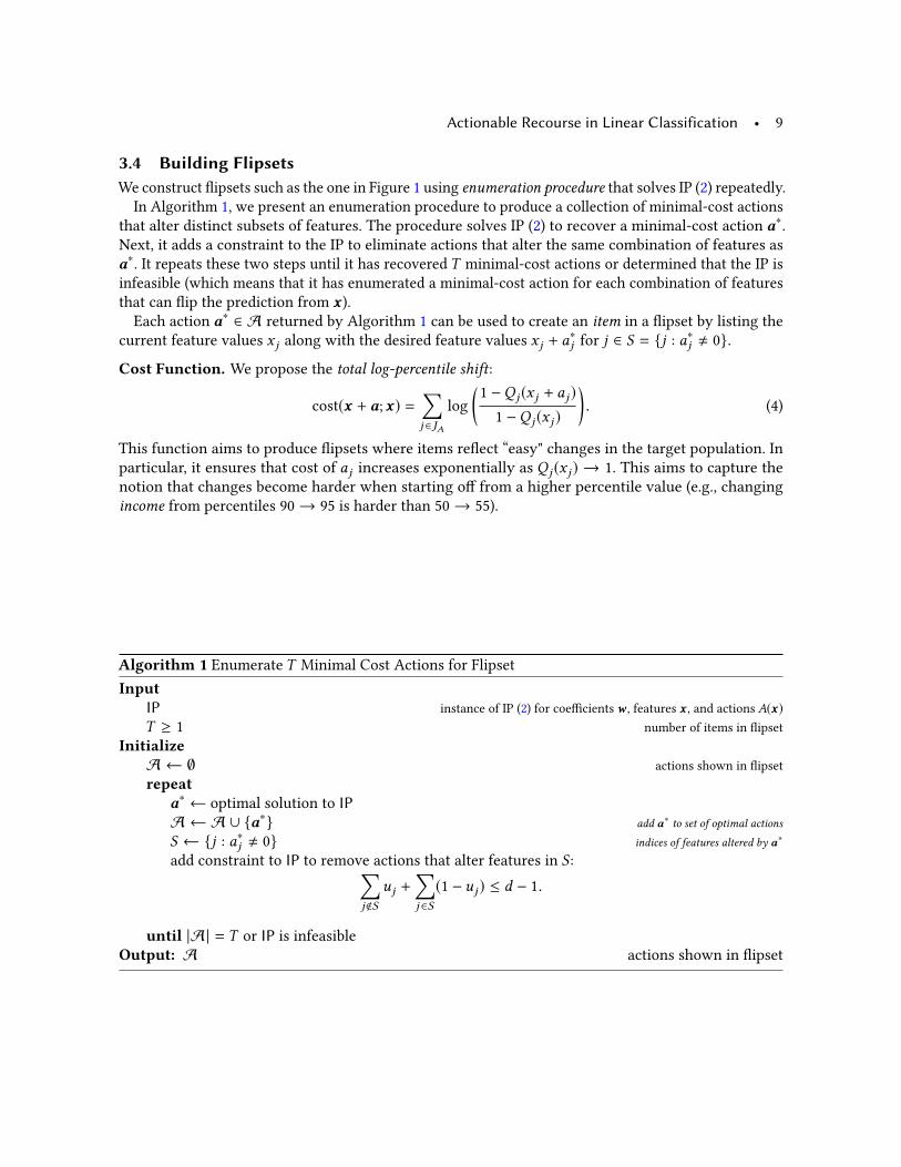
3.4 Building FlipsetsWe construct flipsets such as the one in Figure 1 using enumeration procedure that solves IP (2) repeatedly.In Algorithm 1, we present an enumeration procedure to produce a collection of minimal-cost actions

that alter distinct subsets of features. The procedure solves IP (2) to recover a minimal-cost action a∗.Next, it adds a constraint to the IP to eliminate actions that alter the same combination of features as

a∗. It repeats these two steps until it has recovered T minimal-cost actions or determined that the IP is

infeasible (which means that it has enumerated a minimal-cost action for each combination of features

that can flip the prediction from x ).Each action a∗ ∈ A returned by Algorithm 1 can be used to create an item in a flipset by listing the

current feature values x j along with the desired feature values x j + a∗j for j ∈ S = {j : a∗j , 0}.

Cost Function. We propose the total log-percentile shift:

cost(x + a;x) =∑j ∈JA

log

(1 −Q j (x j + aj )1 −Q j (x j )

). (4)

This function aims to produce flipsets where items reflect “easy" changes in the target population. In

particular, it ensures that cost of aj increases exponentially as Q j (x j ) → 1. This aims to capture the

notion that changes become harder when starting off from a higher percentile value (e.g., changing

income from percentiles 90→ 95 is harder than 50→ 55).

Algorithm 1 Enumerate T Minimal Cost Actions for Flipset

InputIP instance of IP (2) for coefficientsw , features x , and actions A(x)T ≥ 1 number of items in flipset

InitializeA ← ∅ actions shown in flipset

repeata∗ ← optimal solution to IPA ← A ∪ {a∗} add a∗ to set of optimal actions

S ← {j : a∗j , 0} indices of features altered by a∗

add constraint to IP to remove actions that alter features in S :∑j<S

uj +∑j ∈S(1 − uj ) ≤ d − 1.

until |A| = T or IP is infeasible

Output: A actions shown in flipset

10 • Ustun et al.

4 DEMONSTRATIONSIn this section, we present experiments where we use our tools to study recourse in credit scoring

problems. We have two goals: (i) to show how recourse may affected by common practices in the

development and deployment of machine learning models; and (ii) to demonstrate how our tools can

protect recourse in such events by informing stakeholders such as practitioners, policy-makers and

decision-subjects.

In the following experiments, we train classifiers using scikit-learn, and use standard 10-fold cross-

validation (10-CV) to tune free parameters and estimate out-of-sample performance. We solve all IPs

using the CPLEX 12.8 [23] on a 2.6 GHz CPU with 16 GB RAM. We include further information on the

features, action sets, and classifiers for each dataset in Appendix C. We provide scripts to reproduce our

analyses at http://github.com/ustunb/actionable-recourse.

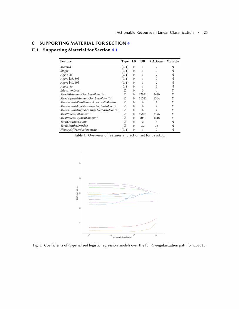
4.1 Model SelectionSetup. We consider a processed version of credit dataset [52]. Here, yi = −1 if person i will defaulton an upcoming credit card payment. The dataset contains n = 30 000 individuals and d = 16 features

derived from their spending and payment patterns, education, credit history, age, and marital status.

We assume that individuals can only change their spending and payment patterns and education.

We train ℓ1-penalized logistic regression models for ℓ

1-penalties of {1, 2, 5, 10, 20, 50, 100, 500, 1000}.

We audit the recourse of each model on the training data, by solving an instance of IP (2) for each iwhere yi = −1. The IP includes the following constraints to ensure changes are actionable: (i) changes

for discrete features must be discrete (e.g. MonthsWithLowSpendingOverLast6Months ∈ {0, 1, . . . , 6});(ii) EducationLevel can only increase; and (iii) immutable features cannot change.

Results. We present the results of our audit in Figure 2, and present a flipset for a person who is denied

credit by the most accurate classifier in Figure 3.

As shown in Figure 2, tuning the ℓ1-penalty has a minor effect on test error, but a major effect on

the feasibility and cost recourse. In particular, classifiers with small ℓ1-penalties provide all individuals

with recourse. As the ℓ1-penalty increases, however, the number of individuals with recourse decreases

as regularization reduces the number of actionable features.

The cost of recourse provides an informative measure of the difficulty of actions. Since we optimize

the cost function in Equation (3), a cost of q implies a person must change a feature by at least qpercentiles to obtain a desired outcome. Here, increasing the ℓ

1-penalty nearly doubles the median cost

of recourse from 0.20 to 0.39. When we deploy a model with a small ℓ1-penalty, the median person with

recourse can only obtain a desired outcome by changing a feature by at least 20 percentiles. At a large

ℓ1-penalty, the median person must change a feature by at least 39 percentiles.

Our aim is not to suggest a relationship between recourse and ℓ1-regularization, but to show how

recourse can be affected by standard tasks in model development such as feature selection and parameter

tuning. Here, a practitioner who aims to maximize performance could deploy a model that precludes

some individuals from achieving a desired outcome (e.g., the one that minimizes mean 10-CV test error),

even as there exist models that perform almost as well but provide all individuals with recourse.

Our tools can identify mechanisms that affect recourse by running audits with different action sets.

For example, one can evaluate how the mutability of feature j affects recourse by running audits for:

(i) an action set where feature j is immutable (Aj (x) = 0 for all x ∈ X); and (ii) an action set where

http://github.com/ustunb/actionable-recourse


feature j is actionable (Aj (x) = Xj for all x ∈ X). Here, such an analysis reveals that the lack of recourse

stems from an immutable feature related to credit history (i.e., an indicator set to 1 if a person has everdefaulted on a loan). Given this information, a practitioner could replace this feature with a mutable

variant (i.e., an indicator set to 1 if a person has recently defaulted on a loan), and thus deploy a model

that provides recourse. Such changes are sometimes mandated by industry-specific regulations [see e.g.,

policies on “forgetfulness" in 8, 18]. Our tools can support these efforts by showing how regulations

would affect recourse in deployment.

100

101

102

103

1-penalty (log scale)

19.0%

19.2%

19.4%

19.6%

19.8%

20.0%

10-C

V M

ean

Test

Err

or

100

101

102

103


0

2

4

6

8

10

12

14

16

Non

-Zer

o C

oeffi

cien

ts

All FeaturesActionable Features

100

101

102

103


0%

20%

40%

60%

80%

100%

% o

f Ind

ivid

uals

with

Rec

ours

e

1-penalty (log scale)0.0

0.2

0.4

0.6

0.8

1.0C

ost o

f Rec

ours

e

Fig. 2. Performance, sparsity, and recourse of ℓ1-penalized logistic regression models for the credit dataset.

We show the mean 10-CV test error (top left), the number of non-zero coefficients (top right), the proportion ofindividuals with recourse in the training data (bottom left), and the distribution of the cost of recourse in thetraining data (bottom right).


MostRecentPaymentAmount $0 −→ $790


MonthsWithZeroBalanceOverLast6Months 1 −→ 2



MonthsWithLowSpendingOverLast6Months 6 −→ 5


MonthsWithLowSpendingOverLast6Months 6 −→ 5


Fig. 3. Flipset for a person who is denied credit by the most accurate classifier built for the credit dataset.Each item shows a minimal-cost action that a person can make to obtain credit.

12 • Ustun et al.

4.2 Out-of-Sample DeploymentWe now discuss an experiment where a classifier is deployed in a setting with dataset shift. Our setup

is inspired by a real-world feedback loop with credit scoring in the United States: young adults often

lack the credit history to qualify for loans, so they are undersampled in datasets that are used to train

a credit score. It is well-known that this kind of systematic undersampling can affect the accuracy

of credit scores for young adults [see e.g., 25, 51]. Here, we show that it can also affect the cost and

feasibility of recourse.

Setup. We consider a processed version of the givemecredit dataset [24]. Here, yi = −1 if person iwill experience financial distress in the next two years. The data contains n = 150 000 individuals and

d = 10 features related to their age, dependents, and financial history. We assume that all features are

actionable except for Age and NumberOfDependents.We draw n = 112 500 examples from the processed dataset to train two ℓ

2-penalized logistic regression

models:

1. Baseline Classifier. This is a baseline model that we train for the sake of comparison. It is trained

using all n = 112 500 examples, which represents the target population.

2. Biased Classifier. This is the model that we would deploy. It is trained using n = 98 120 examples (i.e.,

the 112 500 examples used to train the baseline classifier minus the 14 380 examples with Age < 35).

We compute the cost of recourse using percentile distributions computed from a hold-out set of

n = 37 500 examples. We adjust the threshold of each classifier so that only 10% of examples receive the

desired outcome.

Results. We present the results of our audit in Figure 4 and show flipsets for a prototypical young

adult in Figure 5. As shown, the median cost of recourse among young adults under the biased model is

0.66, which means that the median person can only flip their predictions by a 66 percentile shift in any

feature. In comparison, the median cost of recourse among young adults under the baseline model is

0.14. These differences in the cost of recourse are less pronounced for other age brackets.

Our results illustrate how out-of-sample deployment can significantly affect the cost of recourse.

In practice, such effects can be measured with an audit using data from a target population. Such a

procedure may be useful in model procurement, as classifiers are often deployed on populations that

differ from the population that produced the training data.

There are several ways in which out-of-sample deployment can affect recourse. For example, a

probabilistic classifier may exhibit a higher cost of recourse if the threshold is fixed, or if the target

population has a different set of feasible actions. We controlled for these issues by adjusting thresholds

to approve the same proportion of applicants, and by fixing the action set and cost function to audit both

classifiers. As a result, the observed effects of out-of-sample deployment only depend on distributional

differences in age.


Individuals where y = −1 Individuals where y = +1

Baseline

Classifier

20 30 40 50 60 70 80Age

0.0

0.2

0.4

0.6

0.8

1.0

Cost

of R

ecou

rse

20 30 40 50 60 70 80Age

0.0

0.2

0.4

0.6

0.8

1.0

Cost

of R

ecou

rse

Biased

Classifier

20 30 40 50 60 70 80Age

0.0

0.2

0.4

0.6

0.8

1.0

Cost

of R

ecou

rse

20 30 40 50 60 70 80Age

0.0

0.2

0.4

0.6

0.8

1.0

Cost

of R

ecou

rse

Fig. 4. Distributions of the cost of recourse in the target population for classifiers conditioned on the trueoutcome y. We show the distribution of the cost of recourse for the biased classifier (top) and the baselineclassifier (bottom) for true negatives (left) and false negatives (right). The cost of recourse for young adults issignificantly higher for the biased classifier, regardless of their true outcome.

Baseline Classifier


NumberOfTime30-59DaysPastDueNotWorse 1 −→ 0


NumberRealEstateLoansOrLines 2 −→ 1

NumberOfOpenCreditLinesAndLoans 11 −→ 12

RevolvingUtilizationOfUnsecuredLines 35.89% −→ 36.63%

Biased Classifier

Feature Current Value Reqired Value



Fig. 5. Flipsets for a young adult with Age = 28 under the biased classifier (top) and the baseline classifier(bottom). The flipset for the biased classifier has 1 item while the flipset for the baseline classifier has 4 items.

14 • Ustun et al.

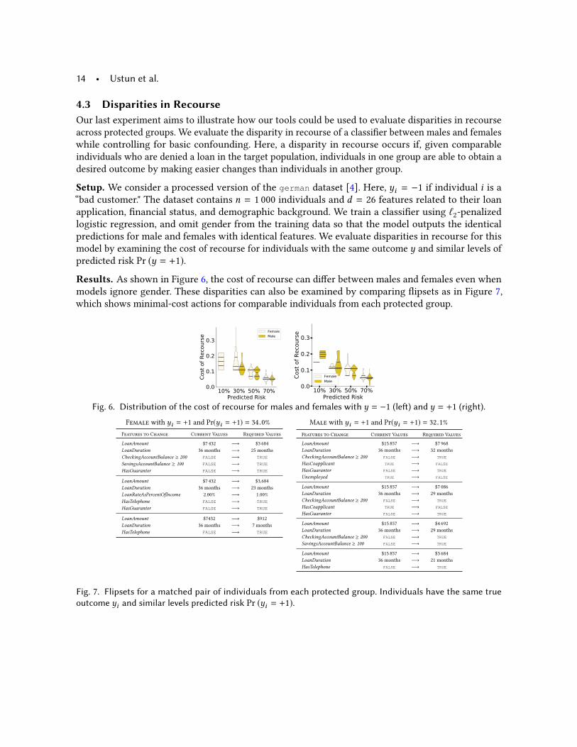
4.3 Disparities in RecourseOur last experiment aims to illustrate how our tools could be used to evaluate disparities in recourse

across protected groups. We evaluate the disparity in recourse of a classifier between males and females

while controlling for basic confounding. Here, a disparity in recourse occurs if, given comparable

individuals who are denied a loan in the target population, individuals in one group are able to obtain a

desired outcome by making easier changes than individuals in another group.

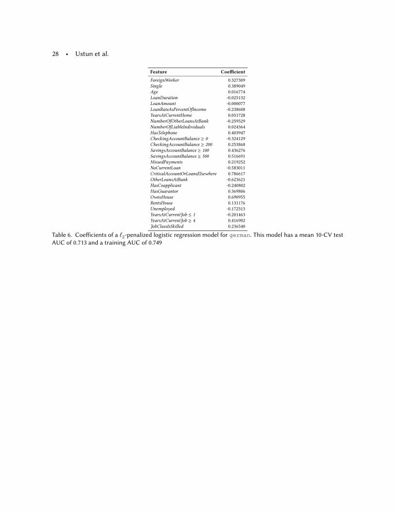
Setup. We consider a processed version of the german dataset [4]. Here, yi = −1 if individual i is a“bad customer." The dataset contains n = 1 000 individuals and d = 26 features related to their loan

application, financial status, and demographic background. We train a classifier using ℓ2-penalized

logistic regression, and omit gender from the training data so that the model outputs the identical

predictions for male and females with identical features. We evaluate disparities in recourse for this

model by examining the cost of recourse for individuals with the same outcome y and similar levels of

predicted risk Pr (y = +1).

Results. As shown in Figure 6, the cost of recourse can differ between males and females even when

models ignore gender. These disparities can also be examined by comparing flipsets as in Figure 7,

which shows minimal-cost actions for comparable individuals from each protected group.

10% 30% 50% 70%Predicted Risk

0.0

0.1

0.2

0.3

Cost

of R

ecou

rse

FemaleMale

10% 30% 50% 70%Predicted Risk

0.0

0.1

0.2

0.3

Cost

of R

ecou

rse

FemaleMale

Fig. 6. Distribution of the cost of recourse for males and females with y = −1 (left) and y = +1 (right).Female with yi = +1 and Pr(yi = +1) = 34.0% Male with yi = +1 and Pr(yi = +1) = 32.1%


LoanAmount $7 432 −→ $3 684

LoanDuration 36 months −→ 25 months

CheckingAccountBalance ≥ 200 FALSE −→ TRUE

SavingsAccountBalance ≥ 100 FALSE −→ TRUE

HasGuarantor FALSE −→ TRUE

LoanAmount $7 432 −→ $3,684


LoanRateAsPercentOfIncome 2.00% −→ 1.00%

HasTelephone FALSE −→ TRUE


LoanAmount $7432 −→ $912




LoanAmount $15 857 −→ $7 968



HasCoapplicant TRUE −→ FALSE


Unemployed TRUE −→ FALSE

LoanAmount $15 857 −→ $7 086



HasCoapplicant TRUE −→ FALSE


LoanAmount $15 857 −→ $4 692



SavingsAccountBalance ≥ 100 FALSE −→ TRUE

LoanAmount $15 857 −→ $3 684



Fig. 7. Flipsets for a matched pair of individuals from each protected group. Individuals have the same trueoutcome yi and similar levels predicted risk Pr (yi = +1).


5 CONCLUDING REMARKS5.1 ExtensionsNon-Linear Classifiers. We are currently extending our tools to evaluate recourse for non-linear

classifiers. One could apply our tools to this setting by replacing the linear classifier with a local

linear model that approximates the decision boundary around x in actionable space [e.g., similar to

the approach used by LIME, 36]. This approach may find actionable changes. However, it would not

provide the proof of infeasibility that is required to claim that a model does not provide recourse.

Pricing Incentives. Our tools could be used to price incentives induced by a model by running audits

with different action sets [see e.g., 26]. Consider a credit score that includes features that are causally

related to creditworthiness (e.g., income) and “ancillary" features that are prone to manipulation (e.g.,

social media presence). In this case, one could price incentives in a target population by comparing the

cost of recourse for actions that alter (i) only causal features, and (ii) causal features and at least one

ancillary feature.

Measuring Flexibility. Our tools can enumerate the complete set of minimal-cost actions for a person

by using the procedure in Algorithm 1 to list actions until the IP become infeasible. This would produce

a collection of actions, where each action reflects a way to obtain the outcome by altering a different

subset of features. The size of this collection would reflect the flexibility of recourse, and may be used

to evaluate other aspects of recourse. For example, if a classifier provides a person with 16 ways to flip

their prediction, 15 of which are legally contestable, then the model itself may be contestable.

5.2 LimitationsAbridged Flipsets. The flipsets in this paper are “abridged" in that they do not reveal all features of

the model. In practice, a person who is shown a flipset in this format may fail to flip their prediction

after making the recommended changes if they unknowingly alter actionable features that are not

shown. This issue can be avoided by including additional information along the flipset – for example, a

list of undisclosed actionable features that must not change, or a list of features that must change in a

certain way. Alternatively, one could also build an abridged flipset with “robust" actions (i.e., actions

that flip the prediction and provide an additional “buffer" to protect against the possibility that a person

alters other undisclosed features in an adversarial manner).

Model Theft. Model owners may not be willing to provide consumers with flipsets due to the potential

for model theft (see e.g., efforts to reverse-engineer the Schufa credit score in Germany by crowdsourcing

[15]). One way to address such concerns would be to produce a lower bound on the number of actions

needed to reconstruct a proprietary model [31, 45]. Such bounds may be useful for quantifying the risk

of model theft, and to inform the design of safeguards to reduce this risk.

5.3 DiscussionWhen Should Models Provide Recourse? Individual rights with regards to algorithmic decision-

making are often motivated by the need for human agency over machine-made decisions. Recourse

reflects a precise notion of human agency – i.e., the ability of a person to alter the predictions of a

model. We argue that models should provide recourse in applications subject to equal opportunity laws

16 • Ustun et al.

(e.g., lending or hiring) and in applications where individuals should have agency over decisions (e.g.,

the allocation of social services).

Recourse provides a useful concept to articulate notions of procedural fairness in applications without

a universal “right to recourse." In recidivism prediction, for example, models should provide defendants

who are predicted to recidivate with the ability to flip their prediction by altering specific sets of features.

For example, a model that includes age and criminal history should allow defendants who are predicted

to recidivate to flip their predictions by “clearing their criminal history." Otherwise, some defendants

would be predicted to recidivate solely on the basis of age.

In settings where recourse is desirable, our tools can check that a model provides recourse through

two approaches: (1) by running periodic recourse audits; and (2) by generating a flipset for every person

who is assigned an undesirable prediction. The second approach has a benefit in that it can detect

recourse violations while a model is deployed. That is, we would know that a model did not provide

recourse to all its decision subjects on the first instance that we would produce an empty flipset.

Should We Inform Consumers of Recourse? In settings where there is an imperative for recourse,

providing consumers with flipsets may lead to harm. Consider a case where a consumer is denied a

loan by a model so that y = −1, and we know that they are likely to default so that y = −1. In this case,

providing them with an action that allows them to flip their prediction from y = −1 to y = +1 couldinflict harm if the action did not also improve their ability to repay the loan from y = −1 to y = +1.Conversely, say that we presented the consumer with an action that allowed them to receive a loan and

also improved their ability to pay it back. In this case, disclosing the action would benefit both parties:

the consumer would receive a loan that they could repay, and the model owner would have improved

the creditworthiness of their consumer.

This example shows how flipsets could benefit all parties if we can find actions that simultaneously

alter their predicted outcome y and true outcome y. Such actions are naturally produced by causal

models. They could also be obtained for predictive models. For example, we could enumerate all actions

that flip the predicted outcome y , then build a filtered flipset using actions that are likely to flip a true

outcome y (e.g., using a technique to estimate treatment effects from observational data).

In practice, the potential drawbacks of gaming have not stopped the development of laws and tools

to empower consumers with actionable information. In the United States, for example, the adverse

action requirement of the Equal Credit Opportunity Act is designed – in part – to educate consumers

on how to obtain credit [see e.g., 43, for a discussion]. In addition, credit bureaus provide credit score

simulators that allow consumers to find actions that will change their credit score in a desired way.2

Policy Implications. While regulations for algorithmic decision-making are still in their infancy,

existing efforts have sought to ensure human agency indirectly, through laws that focus on transparency

and explanation [see e.g., regulations for credit scoring in the United States such as 46]. In light of

these efforts, we argue that recourse should be treated as a standalone policy goal when it is desirable.

This is because recourse is a precise concept with several options for meaningful consumer protection.

For example, one could mandate that a classifier must be paired with a recourse audit for its target

population, or mandate that consumers who are assigned an undesirable outcome are shown a list of

actions to obtain a desired outcome.

2

See, for example, https://www.transunion.com/product/credit-score-simulator.

https://www.transunion.com/product/credit-score-simulator.


ACKNOWLEDGMENTSWe thank the following individuals for helpful discussions: Solon Barocas, Flavio Calmon, Yaron Singer,

Ben Green, Hao Wang, Suresh Venkatasubramanian, Sharad Goel, Matt Weinberg, Aloni Cohen, Jesse

Engreitz, and Margaret Haffey.

REFERENCES[1] Charu C Aggarwal, Chen Chen, and Jiawei Han. 2010. The Inverse Classification Problem. Journal of Computer Science

and Technology 25, 3 (2010), 458–468.

[2] Ifeoma Ajunwa, Sorelle Friedler, Carlos E Scheidegger, and Suresh Venkatasubramanian. 2016. Hiring by Algorithm:

Predicting and Preventing Disparate Impact. Available at SSRN (2016).

[3] Elaine Angelino, Nicholas Larus-Stone, Daniel Alabi, Margo Seltzer, and Cynthia Rudin. 2017. Learning certifiably

optimal rule lists. In Proceedings of the 23rd ACM SIGKDD International Conference on Knowledge Discovery and DataMining. ACM, 35–44.

[4] Kevin Bache and Moshe Lichman. 2013. UCI Machine Learning Repository.

[5] Pietro Belotti, Pierre Bonami, Matteo Fischetti, Andrea Lodi, Michele Monaci, Amaya Nogales-Gómez, and Domenico

Salvagnin. 2016. On handling indicator constraints in mixed integer programming. Computational Optimization andApplications 65, 3 (2016), 545–566.

[6] Reuben Binns, Max Van Kleek, Michael Veale, Ulrik Lyngs, Jun Zhao, and Nigel Shadbolt. 2018. ’It’s Reducing a Human

Being to a Percentage’: Perceptions of Justice in Algorithmic Decisions. In Proceedings of the 2018 CHI Conference onHuman Factors in Computing Systems. ACM, 377.

[7] Or Biran and Kathleen McKeown. 2014. Justification narratives for individual classifications. In Proceedings of the AutoMLworkshop at ICML, Vol. 2014.

[8] Jean-François Blanchette and Deborah G Johnson. 2002. Data retention and the panoptic society: The social benefits of

forgetfulness. The Information Society 18, 1 (2002), 33–45.

[9] Miranda Bogen and Aaron Rieke. 2018. Help wanted: an examination of hiring algorithms, equity, and bias. (2018).

https://www.upturn.org/reports/2018/hiring-algorithms/

[10] Allison Chang, Cynthia Rudin, Michael Cavaretta, Robert Thomas, and Gloria Chou. 2012. How to reverse-engineer

quality rankings. Machine Learning 88, 3 (2012), 369–398.

[11] Alexandra Chouldechova, Diana Benavides-Prado, Oleksandr Fialko, and Rhema Vaithianathan. 2018. A Case Study

of Algorithm-Assisted Decision Making in Child Maltreatment Hotline Screening Decisions. In Conference on Fairness,Accountability and Transparency. 134–148.

[12] Danielle Keats Citron and Frank Pasquale. 2014. The Scored Society: Due Process for Automated Predictions. WashingtonLaw Review 89 (2014), 1.

[13] Bo Cowgill and Catherine E Tucker. 2019. Economics, fairness and algorithmic bias. (2019).

[14] Kate Crawford and Jason Schultz. 2014. Big data and due process: Toward a framework to redress predictive privacy

harms. BCL Rev. 55 (2014), 93.[15] Open Knowledge Foundation Deutschland. 2018. Get Involved: We Crack the Schufa! https://okfn.de/blog/2018/02/

openschufa-english/.

[16] Jinshuo Dong, Aaron Roth, Zachary Schutzman, Bo Waggoner, and Zhiwei Steven Wu. 2018. Strategic Classification

from Revealed Preferences. In Proceedings of the 2018 ACM Conference on Economics and Computation. ACM, 55–70.

[17] Finale Doshi-Velez, Mason Kortz, Ryan Budish, Chris Bavitz, Sam Gershman, David O’Brien, Stuart Schieber, James

Waldo, David Weinberger, and Alexandra Wood. 2017. Accountability of AI Under the Law: The Role of Explanation.

ArXiv e-prints, Article arXiv:1711.01134 (Nov. 2017). arXiv:1711.01134[18] Lilian Edwards and Michael Veale. 2017. Slave to the Algorithm: Why a Right to an Explanation Is Probably Not the

Remedy You Are Looking for. Duke L. & Tech. Rev. 16 (2017), 18.[19] Alhussein Fawzi, Omar Fawzi, and Pascal Frossard. 2018. Analysis of classifiers’ robustness to adversarial perturbations.

Machine Learning 107, 3 (2018), 481–508.

[20] Satoshi Hara, Kouichi Ikeno, Tasuku Soma, and Takanori Maehara. 2018. Maximally Invariant Data Perturbation as

Explanation. arXiv preprint arXiv:1806.07004 (2018).

https://www.upturn.org/reports/2018/hiring-algorithms/

https://okfn.de/blog/2018/02/openschufa-english/

https://okfn.de/blog/2018/02/openschufa-english/

http://arxiv.org/abs/1711.01134

18 • Ustun et al.

[21] Moritz Hardt, Nimrod Megiddo, Christos Papadimitriou, and Mary Wootters. 2016. Strategic Classification. In Proceedingsof the 2016 ACM Conference on Innovations in Theoretical Computer Science. ACM, 111–122.

[22] Lily Hu, Nicole Immorlica, and Jennifer Wortman Vaughan. 2019. The Disparate Effects of Strategic Manipulation.

In Proceedings of the Conference on Fairness, Accountability, and Transparency (FAT* ’19). ACM, New York, NY, USA,

259–268.

[23] IBM ILOG. 2018. CPLEX Optimizer 12.8. https://www.ibm.com/analytics/cplex-optimizer.

[24] Kaggle. 2011. Give Me Some Credit. http://www.kaggle.com/c/GiveMeSomeCredit/.

[25] Nathan Kallus andAngela Zhou. 2018. Residual Unfairness in FairMachine Learning from Prejudiced Data. In InternationalConference on Machine Learning.

[26] Jon Kleinberg and Manish Raghavan. 2018. How Do Classifiers Induce Agents To Invest Effort Strategically? ArXive-prints, Article arXiv:1807.05307 (July 2018), arXiv:1807.05307 pages. arXiv:cs.CY/1807.05307

[27] Brian Y Lim and Anind K Dey. 2009. Assessing demand for intelligibility in context-aware applications. In Proceedings ofthe 11th international conference on Ubiquitous computing. ACM, 195–204.

[28] Dmitry Malioutov and Kush Varshney. 2013. Exact rule learning via boolean compressed sensing. In InternationalConference on Machine Learning. 765–773.

[29] David Martens and Foster Provost. 2014. Explaining data-driven document classifications. MIS Quarterly 38, 1 (2014),

73–100.

[30] Smitha Milli, John Miller, Anca D. Dragan, and Moritz Hardt. 2019. The Social Cost of Strategic Classification. In

Proceedings of the Conference on Fairness, Accountability, and Transparency (FAT* ’19). ACM, New York, NY, USA,

230–239.

[31] Smitha Milli, Ludwig Schmidt, Anca D Dragan, and Moritz Hardt. 2019. Model Reconstruction from Model Explanations.

In Proceedings of the Conference on Fairness, Accountability, and Transparency. ACM, 1–9.

[32] Hans Mittleman. 2018. Mixed Integer Linear Programming Benchmarks (MIPLIB 2010). http://plato.asu.edu/ftp/milpc.

html.

[33] Cathy O’Neil. 2016. Weapons of math destruction: How big data increases inequality and threatens democracy. BroadwayBooks.

[34] Brett Poulin, Roman Eisner, Duane Szafron, Paul Lu, Russell Greiner, David S Wishart, Alona Fyshe, Brandon Pearcy,

Cam MacDonell, and John Anvik. 2006. Visual explanation of evidence with additive classifiers. In Proceedings Of TheNational Conference On Artificial Intelligence, Vol. 21. Menlo Park, CA; Cambridge, MA; London; AAAI Press; MIT Press;

1999, 1822.

[35] Dillon Reisman, Jason Schultz, Kate Crawford, and Meredith Whittaker. 2018. Algorithmic Impact Assessments: A

Practical Framework for Public Agency Accountability. AI Now Technical Report.

[36] Marco Tulio Ribeiro, Sameer Singh, and Carlos Guestrin. 2016. Why should I trust you?: Explaining the predictions of

any classifier. In Proceedings of the 22nd ACM SIGKDD International Conference on Knowledge Discovery and Data Mining.ACM, 1135–1144.

[37] Marco Tulio Ribeiro, Sameer Singh, and Carlos Guestrin. 2018. Anchors: High-precision model-agnostic explanations. In

AAAI Conference on Artificial Intelligence.[38] Leslie Scism. 2019. New York Insurers Can Evaluate Your Social Media Use - If They Can Prove Why It’s Needed.

[39] Ravi Shroff. 2017. Predictive Analytics for City Agencies: Lessons from Children’s Services. Big data 5, 3 (2017), 189–196.[40] Naeem Siddiqi. 2012. Credit Risk Scorecards: Developing and Implementing Intelligent Credit Scoring. Vol. 3. John Wiley &

Sons.

[41] Nataliya Sokolovska, Yann Chevaleyre, and Jean-Daniel Zucker. 2018. A Provable Algorithm for Learning Interpretable

Scoring Systems. In International Conference on Artificial Intelligence and Statistics. 566–574.[42] Alexander Spangher and Berk Ustun. 2018. Actionable Recourse in Linear Classification. In Proceedings of the 5th

Workshop on Fairness, Accountability and Transparency in Machine Learning.[43] Winnie F Taylor. 1980. Meeting the Equal Credit Opportunity Act’s Specificity Requirement: Judgmental and Statistical

Scoring Systems. Buff. L. Rev. 29 (1980), 73.[44] John A Tomlin. 1988. Special ordered sets and an application to gas supply operations planning. Mathematical

programming 42, 1-3 (1988), 69–84.

https://www.ibm.com/analytics/cplex-optimizer

http://www.kaggle.com/c/GiveMeSomeCredit/

http://arxiv.org/abs/cs.CY/1807.05307

http://plato.asu.edu/ftp/milpc.html

http://plato.asu.edu/ftp/milpc.html


[45] Florian Tramèr, Fan Zhang, Ari Juels, Michael K Reiter, and Thomas Ristenpart. 2016. Stealing Machine Learning Models

via Prediction APIs.. In USENIX Security Symposium. 601–618.

[46] United States Congress. 2003. The Fair and Accurate Credit Transactions Act.

[47] United States Senate. 2019. Algorithmic Accountability Act of 2019.

[48] Berk Ustun and Cynthia Rudin. 2016. Supersparse Linear Integer Models for Optimized Medical Scoring Systems.

Machine Learning 102, 3 (2016), 349–391.

[49] Berk Ustun and Cynthia Rudin. 2017. Optimized Risk Scores. In Proceedings of the 23rd ACM SIGKDD InternationalConference on Knowledge Discovery and Data Mining. ACM.

[50] Sandra Wachter, Brent Mittelstadt, and Chris Russell. 2017. Counterfactual Explanations without Opening the Black Box:

Automated Decisions and the GDPR. (2017).

[51] Colin Wilhelm. 2018. Big Data and the Credit Gap. https://www.politico.com/agenda/story/2018/02/07/

big-data-credit-gap-000630.

[52] I-Cheng Yeh and Che-hui Lien. 2009. The Comparisons of Data Mining Techniques for the Predictive Accuracy of

Probability of Default of Credit Card Clients. Expert Systems with Applications 36, 2 (2009), 2473–2480.

https://www.politico.com/agenda/story/2018/02/07/big-data-credit-gap-000630

https://www.politico.com/agenda/story/2018/02/07/big-data-credit-gap-000630

20 • Ustun et al.

A OMITTED PROOFSRemark 1Proof. Given a classifier f : X → {−1,+1}, let us define the space of feature vectors that are assigned

a negative and positive label as H− = {x ∈ X | f (x) = −1} and H+ = {x ∈ X | f (x) = +1}, respectively.Since the classifier f does not trivially predict a single class over the target population, there must exist

at least one feature vector x ∈ H− and at least one feature vector x ′ ∈ H+.Given any feature vector x ∈ H−, choose a fixed point x ′ ∈ H+. Since all features are actionable, the

set of feasible actions from x must contain an action vector a = x ′ − x . Thus, the classifier provides xwith recourse as f (x +a) = f (x +x ′−x) = f (x ′) = +1. Since our choice of x was arbitrary, the previous

result holds for all feature vectors x ∈ H−. Thus, the classifier provides recourse to all individuals in

the target population. □

Remark 2Proof. Given a linear classifier with coefficients w ∈ Rd+1, let j denote the index of feature that

can be increased or decreased arbitrarily. Assume, without loss of generality, that w j > 0. Given a

feature vector x such that f (x) = sign(w⊤x) = −1, the set of feasible actions from x must contain an

action vector a = [0,a1,a

2, . . . ,ad ] such that aj > − 1

w jw⊤x and ak = 0 for all k , j . Thus, the classifier

provides x with recourse asw⊤(x + a) > 0 and f (x + a) = sign(w⊤(x + a)) = +1. Since our choice of xwas arbitrary, the result holds for all x ∈ H−. Thus, the classifier provides recourse to all individuals in

the target population. □

Remark 3Proof. Suppose we have d actionable features x j ∈ {0, 1} for j ∈ {1, . . . ,d} and 1 immutable feature

xd+1 ∈ {0, 1}. Consider a linear classifier with the score function

∑dj=1 x j + αx j+1 ≥ d where α < −1.

For any x with xd+1 = 1, we have that

∑dj=1 x j + αx j+1 <

∑dj=1 x j − 1 ≤ d − 1. Thus, x will not have

recourse. □

Theorem 2.1In what follows, we denote the unit score of actionable features from x as ux =

w⊤AxA| |wA | |22

. Our proof uses

the following lemma from Fawzi et al. [19], which we have reproduced below for completeness:

Lemma A.1 (Fawzi et al. [19]). Given a non-trivial linear classifier wherewA , 0, the optimal cost ofrecourse from x ∈ H− obeys

cost(a∗;x) = cx ·|w⊤AxA || |wA | |22

= cxux .


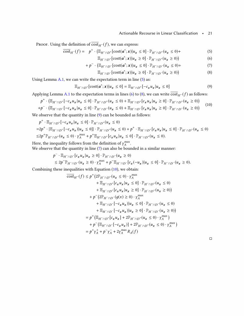
Proof. Using the definition of costH−(f ), we can express:

costH−(f ) = p+ ·(EH−∩D+[cost(a∗;x)|ux ≤ 0] · PH−∩D+(ux ≤ 0)+ (5)

EH−∩D+[cost(a∗;x)|ux ≥ 0] · PH−∩D+(ux ≥ 0))

(6)

+ p− ·(EH−∩D−[cost(a∗;x)|ux ≤ 0] · PH−∩D−(ux ≤ 0)+ (7)

EH−∩D−[cost(a∗;x)|ux ≥ 0] · PH−∩D−(ux ≥ 0))

(8)

Using Lemma A.1, we can write the expectation term in line (5) as:

EH−∩D+[cost(a∗;x)|ux ≤ 0] = EH−∩D+[−cxux |ux ≤ 0] (9)

Applying Lemma A.1 to the expectation terms in lines (6) to (8), we can write costH−(f ) as follows:p+ ·

(EH−∩D+[−cxux |ux ≤ 0] · PH−∩D+(ux ≤ 0) + EH−∩D+[cxux |ux ≥ 0] · PH−∩D+(ux ≥ 0)

)+p− ·

(EH−∩D−[−cxux |ux ≤ 0] · PH−∩D−(ux ≤ 0) + EH−∩D−[cxux |ux ≥ 0] · PH−∩D−(ux ≥ 0)

) (10)

We observe that the quantity in line (9) can be bounded as follows:

p+ · EH−∩D+[−cxux |ux ≤ 0] · PH−∩D+(ux ≤ 0)=2p+ · |EH−∩D+[−cxux )|ux ≤ 0]| · PH−∩D+(ux ≤ 0) + p+ · EH−∩D+[cxux |ux ≤ 0] · PH−∩D+(ux ≤ 0)≤2p+PH−∩D+(ux ≤ 0) · γmax

A + p+EH−∩D+[cxux |ux ≤ 0] · PH−∩D+(ux ≤ 0).Here, the inequality follows from the definition of γmax

A .

We observe that the quantity in line (7) can also be bounded in a similar manner:

p− · EH−∩D−[cxux |ux ≥ 0] · PH−∩D−(ux ≥ 0)≤ 2p−PH−∩D−(ux ≥ 0) · γmax

A + p−EH−∩D−[cx (−ux )|ux ≤ 0] · PH−∩D−(ux ≥ 0).Combining these inequalities with Equation (10), we obtain:

costH−(f ) ≤ p+(2PH−∩D+(ux ≤ 0) · γmax

A

+ EH−∩D+[cxux |ux ≤ 0] · PH−∩D+(ux ≤ 0)+ EH−∩D+[cxux |ux ≥ 0] · PH−∩D+(ux ≥ 0)

)+ p−

(2PH−∩D−(д(x) ≥ 0) · γmax

A

+ EH−∩D−[−cxux )|ux ≤ 0] · PH−∩D−(ux ≤ 0)+ EH−∩D−[−cxux )|ux ≥ 0] · PH−∩D−(ux ≥ 0)

)= p+

(EH−∩D+[cxux ] + 2PH−∩D+(ux ≤ 0) · γmax

A)

+ p−(EH−∩D−[−cxux )] + 2PH−∩D+(ux ≤ 0) · γmax

A)

= p+γ+A + p−γ−A + 2γ

max

A RA(f )□

22 • Ustun et al.

B DISCRETIZATION GUARANTEESIn Section 3, we state that discretization will not affect the feasibility or cost of recourse if we choose a

suitable grid. In what follows, we present formal guarantees for this claim. Specifically, we show that:

1. Discretization does not affect the feasibility of recourse if the actions for real-valued features are

discretized onto a grid with the same upper and lower bounds.

2. The maximum discretization error in the cost of recourse can be bounded and controlled by refining

the grid.

B.1 Feasibility GuaranteeProposition B.1. Given a linear classifier with coefficientsw , consider determining the feasibility of

recourse for a person with features x ∈ X where the set of actions for each feature j belong to a boundedinterval Aj (x) = [amin

j ,amax

j ] ⊂ R. Say we solve an instance of the integer program (IP) (2) using adiscretized action set Adisc(x). If Adisc

j (x) contains the end points of Aj (x) for each j, then the IP will beinfeasible whenever the person does not have recourse.

Proof. When the set of actions for each feature belong to a bounded interval Aj (x) = [amin

j ,amax

j ],we have that:

max

a∈A(x )f (x + a) = max

a∈A(x )w⊤(x + a)

= w⊤x + max

a∈A(x )w⊤a

= w⊤x +∑j ∈JA

max

aj ∈Aj (x )w jaj

= w⊤x +∑

j ∈JA :w j<0

w jamin

j +∑

j :w j>0

w jamax

j

= max

a∈Adisc(x )f (x + a)

Thus, we have shown that:

max

a∈A(x )f (x + a) = max

a∈Adisc(x )f (x + a).

Observe that IP (2) is infeasible whenever maxa∈Adisc(x ) f (x + a) < 0, because this would violate

constraint (2b). Since

max

a∈Adisc(x )f (x + a) < 0⇔ max

a∈A(x )f (x + a) < 0,

it follows that the IP is infeasible whenever the person has no recourse under the original action set. □

B.2 Cost GuaranteeWe present a bound on the maximum error in the cost of recourse due to the discretization of the cost

function cost(a;x) = cx · ∥a∥, where c : X → (0,+∞) is a strictly positive scaling function for actions

from x . Given a feature vector x ∈ X, we denote the discretized action set from x as A(x) and the


continuous action set as B(x). We denote the minimal-cost action over A(x) as:

a∗ ∈ argmin cx · | |a | |s.t. f (x + a) = 1

a ∈ A(x)(11)

and the minimal-cost action over B(x) as:

b∗ ∈ argmin cx · | |b | |s.t. f (x + b) = 1

b ∈ B(x)(12)

We assume that A(x) ⊆ {a ∈ Rd | aj ∈ Aj (x j )} and denote the feasible actions for feature j asAj (x j ) = {0,aj1, ...,aj,mj

}.We measure the refinement of the discrete grid in terms of the maximumdiscretization gap: √∑

j ∈Jδ 2j .

Here δ j = maxk=0, ..,mj−1 |aj,k+1 − aj,k |. In Proposition B.2, we show that the difference in the cost of

recourse due to discretization can be bounded in terms of the maximum discretization gap.

Proposition B.2. Given a linear classifier with coefficientsw , consider evaluating the cost of recoursefor an individual with features x ∈ X. If the features belong to a bounded space x ∈ X, then the cost canbe bounded as:

cx · | |a∗ | | − cx · | |b∗ | | ≤ cx ·

√√√ d∑j=1

δ 2j .

Proof. Let N (b∗) be a neighborhood of real-valued vectors centered at x +b∗ and with radius

∑dj=1 δ j :

N (b∗) =x ′ :

x ′ − (x + b∗) ≤ √√√ d∑j=1

δ 2j

.Observe that N (b∗)must contain an action a ∈ A(x) such that f (x + a) = +1. By the triangle inequality,we can see that:

∥a∥ ≤ b∗ + a − b∗ ,≤ b∗ +√√√ d∑

j=1

δ 2j . (13)

24 • Ustun et al.

Here the inequality in (13) follows from the fact that x + a ∈ N (b∗). Since a∗ is optimal, we have that a∗ ≤ ∥a∥. Thus we have,cx · | |a∗ | | − cx ·

b∗ ≤ cx · | |a | | − cx · b∗

≤ cx ·

√√√ d∑j=1

δ 2j .

□

B.3 IP Formulation without DiscretizationIn what follows, we present an IP formulation that does not require discretizing real-valued features,

which we mention in Section 3. Given a linear classifier with coefficientsw = [w0, . . . ,wd ] and a person

with features x = [1,x1, . . . ,xd ], we can recover the solution to the optimization problem in (1) for a

linear cost function with the form cost(a;x) = ∑j c jaj , by solving the IP:

min cost

s.t. cost =∑j ∈J

c jaj (14a)

∑j ∈JA

w jaj ≥ −d∑j=0

w jx j (14b)

aj ∈ [amin

j ,amax

j ] j ∈ Jcts

(14c)

aj =

mj∑k=1

ajkvjk j ∈ Jdisc

1 = uj +

mj∑k=1

vjk j ∈ Jdisc

(14d)

aj ∈ R j ∈ Jdisc

uj ∈ {0, 1} j ∈ Jdisc

vjk ∈ {0, 1} k = 1, . . . ,mj j ∈ Jdisc

Here, we denote the indices of actionable features as JA = Jcts∪ J

disc, where J

ctsand J

disccorrespond to

the indices of real-valued features and discrete-valued features, respectively. This formulation differs

from the discretized formulation in Section 3 in that: (i) it represents actions for real-valued features via

continuous variables aj ∈ [amin

j ,amax

j ] in (14c); (ii) it only includes indicator variables uj and vjk and

constraints (14d) for discrete-valued variables j ∈ Jdisc

;

The formulation in (14) has the following drawbacks:

1. It forces users to use linear cost functions. This significantly restricts the ability of users to specify

useful cost functions. Examples include cost functions based on percentile shifts, such as those in (3)

and (4), which are non-convex.

2. It is harder to optimize when we introduce constraints on feasible actions. If we wish to limit the

number of features that can be altered in IP (14), for example, we must add indicator variables of

the form uj = 1[aj , 0] for real-valued features j ∈ Jcts. These variables must be set via “Big-M"

constraints, which produce weak LP relaxations and numerical instability [see e.g., 5, for a discussion].


C SUPPORTING MATERIAL FOR SECTION 4C.1 Supporting Material for Section 4.1

Feature Type LB UB # Actions Mutable

Married {0, 1} 0 1 2 N

Single {0, 1} 0 1 2 N

Age < 25 {0, 1} 0 1 2 N

Age ∈ [25, 39] {0, 1} 0 1 2 N

Age ∈ [40, 59] {0, 1} 0 1 2 N

Age ≥ 60 {0, 1} 0 1 2 N

EducationLevel Z 0 3 4 Y

MaxBillAmountOverLast6Months Z 0 17091 3420 Y

MaxPaymentAmountOverLast6Months Z 0 11511 2304 Y

MonthsWithZeroBalanceOverLast6Months Z 0 6 7 Y

MonthsWithLowSpendingOverLast6Months Z 0 6 7 Y

MonthsWithHighSpendingOverLast6Months Z 0 6 7 Y

MostRecentBillAmount Z 0 15871 3176 Y

MostRecentPaymentAmount Z 0 7081 1418 Y

TotalOverdueCounts Z 0 2 3 N

TotalMonthsOverdue Z 0 32 33 N

HistoryOfOverduePayments {0, 1} 0 1 2 N

Table 1. Overview of features and action set for credit.

Fig. 8. Coefficients of ℓ1-penalized logistic regression models over the full ℓ

1-regularization path for credit.

26 • Ustun et al.

C.2 Supporting Material for Section 4.2


RevolvingUtilizationOfUnsecuredLines R 0.0 1.1 101 Y

Age Z 24 87 64 N

NumberOfTimes30-59DaysPastDueNotWorse Z 0 4 5 Y

DebtRatio R 0.0 5003.0 101 Y

MonthlyIncome Z 0 23000 101 Y

NumberOfOpenCreditLinesAndLoans Z 0 24 25 Y

NumberOfTimes90DaysLate Z 0 3 4 Y

NumberRealEstateLoansOrLines Z 0 5 6 Y

NumberOfTimes60-89DaysPastDueNotWorse Z 0 2 3 Y

NumberOfDependents Z 0 4 5 N

Table 2. Overview of features and actions for givemecredit.

Feature Coefficient

RevolvingUtilizationOfUnsecuredLines 0.000060

Age 0.038216

NumberOfTime30-59DaysPastDueNotWorse -0.508338

DebtRatio 0.000070

MonthlyIncome 0.000036

NumberOfOpenCreditLinesAndLoans 0.010703

NumberOfTimes90DaysLate -0.374242

NumberRealEstateLoansOrLines -0.065595

NumberOfTime60-89DaysPastDueNotWorse 0.852129

NumberOfDependents -0.067961

Table 3. Coefficients of the baseline ℓ2-penalized logistic regression model for givemecredit. This classifier is

trained on a representative sample from the target population. It has a mean 10-CV AUC of 0.693 and a trainingAUC of 0.698.

Feature Coefficient

RevolvingUtilizationOfUnsecuredLines 0.000084

Age 0.048613

NumberOfTime30-59DaysPastDueNotWorse -0.341624

DebtRatio 0.000085

MonthlyIncome 0.000036

NumberOfOpenCreditLinesAndLoans 0.005317

NumberOfTimes90DaysLate -0.220071

NumberRealEstateLoansOrLines -0.037376

NumberOfTime60-89DaysPastDueNotWorse 0.337424

NumberOfDependents -0.008662

Table 4. Coefficients of the biased ℓ2-penalized logistic regression model for givemecredit. This classifier is

trained on the biased sample that undersamples young adults in the target population. It has a mean 10-CV testAUC of 0.710 and a training AUC of 0.725.


C.3 Supporting Material for Section 4.3


ForeignWorker {0, 1} 0 1 2 N

Single {0, 1} 0 1 2 N

Age Z 20 67 48 N

LoanDuration Z 6 60 55 Y

LoanAmount Z 368 14318 101 Y

LoanRateAsPercentOfIncome Z 1 4 4 Y

YearsAtCurrentHome Z 1 4 4 Y

NumberOfOtherLoansAtBank Z 1 3 3 Y

NumberOfLiableIndividuals Z 1 2 2 Y

HasTelephone {0, 1} 0 1 2 Y

CheckingAccountBalance ≥ 0 {0, 1} 0 1 2 Y

CheckingAccountBalance ≥ 200 {0, 1} 0 1 2 Y

SavingsAccountBalance ≥ 100 {0, 1} 0 1 2 Y

SavingsAccountBalance ≥ 500 {0, 1} 0 1 2 Y

MissedPayments {0, 1} 0 1 2 Y

NoCurrentLoan {0, 1} 0 1 2 Y

CriticalAccountOrLoansElsewhere {0, 1} 0 1 2 Y

OtherLoansAtBank {0, 1} 0 1 2 Y

HasCoapplicant {0, 1} 0 1 2 Y

HasGuarantor {0, 1} 0 1 2 Y

OwnsHouse {0, 1} 0 1 2 N

RentsHouse {0, 1} 0 1 2 N

Unemployed {0, 1} 0 1 2 Y

YearsAtCurrentJob ≤ 1 {0, 1} 0 1 2 Y

YearsAtCurrentJob ≥ 4 {0, 1} 0 1 2 Y

JobClassIsSkilled {0, 1} 0 1 2 N

Table 5. Overview of features and actions for german.

28 • Ustun et al.

Feature Coefficient

ForeignWorker 0.327309

Single 0.389049

Age 0.016774

LoanDuration -0.025132

LoanAmount -0.000077

LoanRateAsPercentOfIncome -0.238608

YearsAtCurrentHome 0.051728

NumberOfOtherLoansAtBank -0.259529

NumberOfLiableIndividuals 0.024364

HasTelephone 0.403947

CheckingAccountBalance ≥ 0 -0.324129

CheckingAccountBalance ≥ 200 0.253868

SavingsAccountBalance ≥ 100 0.436276

SavingsAccountBalance ≥ 500 0.516691

MissedPayments 0.219252

NoCurrentLoan -0.583011

CriticalAccountOrLoansElsewhere 0.786617

OtherLoansAtBank -0.623621

HasCoapplicant -0.240802

HasGuarantor 0.369806

OwnsHouse 0.690955

RentsHouse 0.131176

Unemployed -0.172313

YearsAtCurrentJob ≤ 1 -0.201463

YearsAtCurrentJob ≥ 4 0.416902

JobClassIsSkilled 0.236540

Table 6. Coefficients of a ℓ2-penalized logistic regression model for german. This model has a mean 10-CV test

AUC of 0.713 and a training AUC of 0.749

BERK USTUN, ALEXANDER SPANGHER, University of Southern ...

Documents

Transcript of BERK USTUN, ALEXANDER SPANGHER, University of Southern ...