Institut f. Statistik u. Wahrscheinlichkeitstheorie

1040 Wien, Wiedner Hauptstr. 8-10/107

AUSTRIA

http://www.statistik.tuwien.ac.at

Benefits from using continuous rating scales

in online survey research

H. Treiblmaier and P. Filzmoser

Forschungsbericht SM-2009-4November 2009

Kontakt: P.Filzmoser@tuwien.ac.at

1

Benefits from Using Continuous Rating Scales in Online Survey Research

Horst Treiblmaier*

Institute for Management Information Systems

Vienna University of Economics and Business

Augasse 2-6, 1090 Vienna, Austria1

Peter Filzmoser

Department of Statistics and Probability Theory

Vienna University of Technology

Wiedner Hauptstraße 8-10, A-1040 Vienna, Austria

Abstract The usage of Likert-type scales has become widespread practice in current IS research.

Those scales require individuals to choose between a limited number of choices, and have

been criticized in the literature for causing loss of information, allowing the researcher to af-

fect responses by determining the range, and being ordinal in nature. The use of online sur-

veys allows for the easy implementation of continuous rating scales, which have a long histo-

ry in psychophysical measurement but were rarely used in IS surveys. This type of mea-

surement requires survey participants to express their opinion in a visual form, i.e. to place a

mark at an appropriate position on a continuous line. That not only solves the problems of

information loss, but also allows for applying advanced robust statistical analyses. In this

1 Augasse 2-6, A-1090 Vienna, Austria

Tel.: +43/1/31336/4480

Fax: +43/1/31336/746

E-Mail: Horst.Treiblmaier@wu.ac.at

2

paper we use a real-world sample and a simulation to illustrate how noise impacts our data

set. A noise level of 10% has only a small effect on both classical and robust estimates, but

when 20% of noise is added, the classical estimators become severely distorted. Continuous

rating scales in combination with robust estimators turn out to be an effective tool to reduce

the impact of noise in surveys.

Keywords: Measurement, Scaling, Continuous Rating Scale, Online Research, Robust Cor-

relation, Factor Analysis, MCD estimator

Introduction The concept of measurement is fundamental to all empirical social science research, includ-

ing Information Systems and closely related disciplines such as Marketing and Psychology.

Given its widespread and frequent application in countless studies, it seems peculiar that

Allport and Kerler (2003, p. 356) caution that „measurement is perhaps the most difficult as-

pect of behavioral research‟. The classic definition of measurement was given by Stevens

(1946), who described it as the assignment of numerals to events or objects according to

rules. This definition has been criticized over the last few decades, as for instance by Mitchell

(1999), who argues that there is a difference between the traditional understanding of mea-

surement in the natural sciences and Steven‟s definition. The first pertains to „the discovery

of real numeric relations (ratios) between things (magnitudes of attributes), and not the at-

tempt to construct conventional numerical relations where they do not otherwise exist‟ (Mit-

chell, 1999, p. 17, cited in Balnaves & Caputi, 2001). Accordingly, the two main tasks of

quantitative science are to (1) make sure that the attribute under investigation is in fact quan-

titative and (2) devise procedures to measure the magnitude of this attribute. It can easily be

seen that in social science research the first assumption is an essential precondition for all

further analyses. Balnaves and Caputi (p. 51) give the examples of self-esteem and extro-

version, but quantifiability is also implicitly taken for granted for all the constructs being fre-

quently used in IS research. The second task, albeit being important, is scarcely a topic of

3

interest in IS literature. A plethora of research on how to build valid and reliable constructs

exists (e.g. Straub, 1989; Moore & Benbasat, 1991; Salisbury et al., 2002; Straub et al.,

2004; Lewis, 2005; Huang, 2005), but the core process of measurement itself is largely ig-

nored by IS researchers. In most empirical behavioral IS studies, Likert-type scales are used

to measure individuals‟ attitudes but the rationale for choosing a particular type of scaling is

hardly ever given.

The most frequently used classification of measurement scales distinguishes between four

different levels of measurement (nominal, ordinal, interval and ratio), which in turn impact the

statistical techniques that can be applied (Stevens, 1946). The nominal scale is a system of

classification (i.e. a categorical scale), the ordinal scale involves some ranking, but only in

the interval and ratio scales will the difference between two variables becomes meaningful.

Accordingly, it is only with these latter two scales „that researchers can justify the use of the

arithmetic mean as the measure of average‟ (Coldwell & Herbst, 2004, p. 65). An illustrating

example is given by Allen and Seaman (2007). They use data from an Alfred P. Sloan survey

in which users compare the outcomes from online learning to face-to-face learning on a 5-

point Likert scale. 1.8% of the respondents considered online learning to be „superior‟, 15.1%

„somewhat superior‟, 45% „the same‟, 30.3% „somewhat inferior‟ and 7.8% „inferior‟. A total of

61.9% of the respondents therefore perceived online learning to be equal or superior to face-

to-face learning. However, the mean value is 2.7, indicating a lower than average level of

agreement. As a solution, the authors recommend using a continuous line or track bar, which

allows for an interval measure. This type of measurement was used in IS research before

(Treiblmaier et al., 2004), but has not gained widespread acceptance. Above all, its specific

properties have not yet been fully exploited, which can be partially attributed to a shortage of

easily available statistical methods in the past and a lack of awareness on the side of the

researchers.

In the following sections we will first discuss the properties of various measurement scales

and subsequently focus on the continuous rating scale in online surveys in more detail. Sub-

4

sequently we discuss the problem of outliers and nonsense data in survey research and ap-

ply classical and robust factor analysis to our data sample. Finally, we simulate the occur-

rence of outliers („noise‟) in our data set and illustrate how different levels of noise impact the

results of factor analytic procedures.

Measurement Scaling

The usage of surveys in IS research has been heavily criticized in the past for lack of psy-

chometric rigor and appropriate modeling techniques. In order to remedy this problem, gen-

eral standards for conducting surveys have to be improved and constantly questioned (Pin-

sonneault & Kraemer, 1993; Newsted et al., 1996). When constructing a questionnaire, re-

searchers are confronted with the task of finding an appropriate scale to measure the con-

struct(s) under investigation. Usually this is done by consulting previous literature and adopt-

ing a set of items which has been previously tested for validity and reliability. A classical pro-

cedure for developing constructs is the Multitrait-Multimethod Matrix (Campbell & Fiske,

1959), which ensures that constructs which theoretically should be related are in reality inter-

related (convergent validity), and constructs which theoretically should not be related are not

in reality related (discriminant validity). Due to the many problems which occurred with this

technique, alternative approaches have been developed (for an overview see Straub et al.,

2004). However, by using previously tested scales, researchers ensure validity and reliability,

but this does not guarantee that the data being generated are well-suited for all subsequent

procedures, i.e. that they comply with the statistical techniques being used. Accordingly,

Smith and Albaum (2005) list a total of nine issues which should be considered when con-

structing a measurement scale, including the number of categories, the decision whether an

odd or even number should be chosen, the selection of descriptive adjectives and the proce-

dure being used to account for raters‟ bias.

5

Previous research has highlighted the problem that Likert-type scales in social science re-

search are in fact categorical, i.e. that they consist of a fixed number of responses, but re-

searchers treat them as though they are interval scaled. Since such data are not normally

distributed, the questions arise as to whether „continuous normal theory-based estimators

such as maximum likelihood and generalized least square can recover the parameters of

models estimated on such data and whether standard errors and test statistics are unduly

affected by non-normality induced by categorization and skewness‟ (Kaplan, 2000, p. 83).

These problems become even more pronounced when researchers assign labels to the indi-

vidual categories (Kolic, 2004). Zeis et al. (2001) use the minimum chi-square method to fit

484 5-point Likert scale variables from various Management and Marketing surveys to differ-

ent distributions (normal, lognormal, beta, gamma and Weibull). They conclude that „49% of

the 484 variables were found to “not unreasonably” fit at least one of the five distributions,

using a significance level of 20% (p. 36f)‟. However, in a reverse conclusion, this means that

51% of the variables did not fit.

An ordinal level of measurement leads to several limitations for subsequent analyses. First, it

only allows for the use of statistical techniques which do not rely on the arithmetic mean.

Second, the labels being chosen by the researchers tend to influence the subjects‟ res-

ponses (Lodge, 1981). Third, information might be lost due to the limited resolution of the

categories and fourth, by constraining or expanding the range which can be used, the inves-

tigator may influence response behavior (Neibecker, 1984).

Figure 1 illustrates the difference between various measurement techniques by using exam-

ples from IS research. The sample item for the 7-point Likert scale for measuring perceived

usefulness and the semantic differential item for measuring perceived enjoyment in the top

row come from Igbaria et al. (1995). The integer scale (bottom, left) was used by Palmer

(2002) to assess Web usability and the continuous rating scale was designed by Stanley and

Jenkins (2007). The latter is basically a bipolar graphic rating scale with two fixed points on

either end, represented as a line (Brace, 2004). It can be seen that the classic Likert scale in

6

the upper left corner is the most problematic one when it comes to the distance between the

various categories. In contrast, an interval-level scale has equidistant intervals, i.e. informa-

tion not only about the rank of a particular score is given, but also on how much greater or

less a particular score is than another (Pett, 1997).

Likert (1932) himself argued that the distances of scores such as 1, 2, 3, 4, 5 are equal and

yield data which are approximately normally distributed. The question is if the same is true

for the labels (e.g. „Strongly Agree‟) which are frequently used. Recent research suggests

that literacy affects the ability to discriminate between categories, i.e. that the suitability of the

classical Likert scale depends on the choice of the sample (Chachamovich et al. 2009).

In the other three scales in Figure 1 (semantic differential, integer scale and continuous rat-

ing scale), only the anchor points are given and it is up to the respondent to pick any value in

between. In this case, the semantic understanding of the various categories is less important

(as long as the anchor points are clearly defined). The higher the numbers of categories the

more the categorical scales resemble a continuous rating scale.

Figure 1 Types of Measurement Scales (cf. Smith et al., 2005; Igbaria et al., 1995; Palmer,

2002; Stanley & Jenkins, 2007)

7

Online surveys with Continuous Rating Scales

The problem of inadequate scaling, which we discussed in the previous section, can be easi-

ly overcome by using online (or at least computer-administrated) surveys with continuous

scales. Before discussing a practical application which can be used for sophisticated statis-

tical analyses, we have to deal with two problems. First, we have to investigate if online sur-

veys can substitute offline surveys in general and second, we have to take a closer look at

the characteristics of continuous scales and the rationale behind them.

The relative ease of use of computers for conducting surveys has lead to the proliferation of

computer-administered surveys which soon caught the interest of researchers. Previous stu-

dies have shown that in carefully designed surveys the choice of the medium does not affect

the results (Hays & MacCallum, 2005). Similar research has highlighted the viability of the

Internet for conducting online research (Fouladi et al., 2002; Gosling et al. 2004). Stanley

and Jenkins (2007) investigated the general acceptance of graphical image-based controls

for collecting web survey data and concluded that „many respondents across all ages […]

found the graphical inputs acceptable, enjoyed completing the questionnaire and were look-

ing forward to more surveys of this type in the future‟. Furthermore, they „found no significant

disadvantage of graphical scales for response rates or completion times‟ (p. 92). Previously,

the use of continuous scales was impractical, since the positions marked on questionnaires

had to be measured manually, which was cost-intensive and inaccurate. Online surveys have

made this problem obsolete (Brace, 2004).

As we have previously discussed above, measurements can be seen as the discovery of

numeric relations between magnitudes of attributes. Using continuous scales, which are also

labeled as graphic rating scales, not only allows for generating interval-scaled data, but also

avoids the cognitive effort of matching semantic statements with numbers. Instead, such

scales rely on the effect of visual stimuli, or, as is nicely described in the definition of psycho-

physics, they allow for „the analysis of perceptual processes by studying the effect on a sub-

ject‟s experience or behavior of systematically varying the properties of a stimulus along one

8

or more physical dimensions‟ (Bruce et al., 2003, p. 462). In the 1950s, S.S. Stevens devel-

oped power law scales of various sensations with k , where is the magnitude of a

sensation, is the intensity of the stimulus, indicates the growth of the sensation when

the stimulus increases and k is a constant (Stevens, 1975). A well-known example is the

measurement of the perception of loudness, which typically yields a smaller than one,

which indicates that the perception increases at a slower rate than the actual sound pressure

level (Shofner & Selas, 2002). Neibecker (1984) has shown that continuous scales (he calls

them „magnitude scales‟ and used the length of a line to measure the attitudes toward pic-

tures) are a valid and reliable alternative to rating scales and can be successfully used in

Marketing Research. We will illustrate that the advent and advancement of robust statistical

techniques in combination with computer technology have vastly improved the usability and

explanatory power of those scales in recent years.

Outliers and Nonsense Data in Survey-Based Research

Survey-based research depends on the quality of the data, i.e. the „fitness for use‟ (Juran,

1988) of the data to answer the research question at hand. Various factors exist which im-

pact the accuracy and completeness of the data. Apart from technical problems and errors

on the side of the researcher, incorrect data entries may be caused by the survey respon-

dent, either intentionally or unintentionally. Ironically, unintentional „misresponses‟ might be

due to the usage of reversed Likert items, which occasionally are added to serve as control

questions. This can be attributed to the complexity of cognitive operations, which is neces-

sary for a respondent to compare a scale item with his own beliefs (Swain et al., 2008). Then

again, the respondent might decide to incorrectly fill out questions either because of lack of

knowledge, unwillingness to give away certain types of data (Wentland and Smith, 1993), or

simply by erratically filling out the survey. The latter might be of importance when respon-

dents are „forced‟ to complete a questionnaire (e.g. students who have to complete an as-

9

signment) or when incentives are given. All these situations lead to outliers, i.e. data records

which are inconsistent with the remainder of the observations in that data set. Such data are

problematic since they are not indicative of future behavior of data sets from the same

source (Hazewinkel, 2002). Outliers can be univariate (i.e. they occur within a single varia-

ble) or multivariate (occur within a combination of variables). Various statistical techniques

exist for outlier detection (e.g. the interquartile range for univariate and the Mahalanobis dis-

tance for multivariate outliers), however, those procedures are seldom applied in social

science research. Some authors also refer to problematic data as noise or „nonsense data‟,

i.e. data which „are low in practical value for decision making and are unreliable and internal-

ly and/or externally invalid‟ (Schutz, 1999, p. 246).

The reason for this lack of outlier identification is twofold. First, Likert-type scales allow only

for a limited number of response categories, which makes it virtually impossible to identify

univariate outliers by using the interquartile range. Second, the item sets are frequently ar-

ranged in groups according to the constructs being used. If a respondent fills out the ques-

tionnaire sloppily (i.e. uses the same response category over and over again), no outliers will

be detected as long as reversed coding is not used. Even worse, the frequently used Cron-

bach‟s Alpha (which is in fact a measure of internal consistency) will indicate a high level of

reliability, which is desired by the researchers. The scale level and the research design

therefore impede the application of one of the many outlier detection methodologies being

available (Hodge & Austin, 2004).

Method Classical and robust correlation

Outliers or noise in the data affect the estimation of the correlation coefficient. Consequently,

statistical methods which are based on correlation estimates, such as principal component or

factor analysis, or structural equation models can lead to erroneous results. As a solution,

10

robust estimates of correlation can be used, yielding reliable results despite the presence of

noise and outliers.

In the literature several robust covariance and correlation estimators have been proposed.

Among the desirable properties of such estimates are affine equivariance, high efficiency,

and a high breakdown point, but also a fast algorithm for its computation (Maronna et al.,

2006). The MCD (Minimum Covariance Determinant) estimator (Rousseeuw & Van Driessen,

1999) achieves these goals; it is implemented in various statistical software packages and

thus also frequently applied. The MCD estimator looks for a subset h out of all n observations

with the smallest determinant of their sample covariance matrix. A robust estimator of loca-

tion is the arithmetic mean of these observations, and a robust estimator of covariance is the

sample covariance matrix of the h observations, multiplied by a factor for consistency at nor-

mal distributions. The subset size h can vary between half the sample size and n, and it will

determine not only the robustness of the estimates, but also their efficiency.

The definition of the objective function of the MCD estimator already reveals potential difficul-

ties with categorical data, such as data originating from a 5-point Likert scale. With only a

limited number of categories, it can happen that h observations are arranged on a subspace

of the p-dimensional space spanned by the p variables. For example, this occurs if at least h

values of one variable are equal, but also more complex situations can lead to this artifact.

As a consequence, the sample covariance matrix of these h observations is singular and its

determinant is zero, leading to an ill-conditioned minimization problem of the MCD. Increas-

ing the number of categories in the scale to be used for the questionnaires will reduce the

probability of singularity. As an example, a scale with categories 1, 2, ..., 100 reduces the risk

of singularity considerably.

An example of a two-dimensional case is given in Figure 2. On the left side, 100 artificial data

points on a scale from 1 to 100 (in steps of 1) are presented. The points marked with crosses

are multivariate outliers, because they do not follow the trend of the majority of the data. Note

that these outliers are not visible when inspecting the single variables, and thus they are truly

11

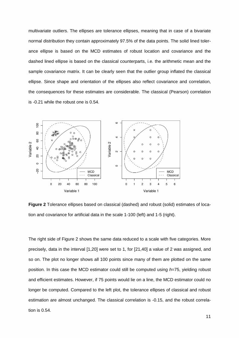
multivariate outliers. The ellipses are tolerance ellipses, meaning that in case of a bivariate

normal distribution they contain approximately 97.5% of the data points. The solid lined toler-

ance ellipse is based on the MCD estimates of robust location and covariance and the

dashed lined ellipse is based on the classical counterparts, i.e. the arithmetic mean and the

sample covariance matrix. It can be clearly seen that the outlier group inflated the classical

ellipse. Since shape and orientation of the ellipses also reflect covariance and correlation,

the consequences for these estimates are considerable. The classical (Pearson) correlation

is -0.21 while the robust one is 0.54.

Figure 2 Tolerance ellipses based on classical (dashed) and robust (solid) estimates of loca-

tion and covariance for artificial data in the scale 1-100 (left) and 1-5 (right).

The right side of Figure 2 shows the same data reduced to a scale with five categories. More

precisely, data in the interval [1,20] were set to 1, for [21,40] a value of 2 was assigned, and

so on. The plot no longer shows all 100 points since many of them are plotted on the same

position. In this case the MCD estimator could still be computed using h=75, yielding robust

and efficient estimates. However, if 75 points would lie on a line, the MCD estimator could no

longer be computed. Compared to the left plot, the tolerance ellipses of classical and robust

estimation are almost unchanged. The classical correlation is -0.15, and the robust correla-

tion is 0.54.

12

Thus, in this example the scale 1 to 5 has little effect on the correlation estimates, but the

outliers severely affected the classical estimates in both cases. As mentioned above, robust

MCD estimation is often not possible with a scale with only a few categories because of sin-

gularity problems, and other robust estimates of location and covariance, such as S-

estimates (Davies, 1987) have similar limitations. In general, the scale 1-100 does not pro-

vide better precision or more relevant information, but it can be helpful for avoiding singularity

problems. Moreover, this scale may be helpful for approaching normal distribution, an impor-

tant assumption of most correlation based methods.

Development of a Continuous Rating Scale and Data Collection

Creating and improving the scales for our research was a multi-step process. We developed

a slider bar with the help of JavaScript. The data gathering process was straightforward. A

HTML form submitted the information using the POST method. A Perl script was used for

reading the data which were subsequently stored in a MYSQL database. By eliminating all

human interference from the process of data collection and storage, we were able to get rid

of an important source of error. However, we needed several pretests and studies to figure

out the best version of the slider bar. The main issues included the implementation of a „de-

fault position‟ of the slider, the length of the scale and the general usability of this type of

measurement.

We started with a range of 101 pixels and tested it under various conditions (screen size,

screen resolution). The first version of our questionnaire had the slider as a „default option‟,

i.e. it was initially placed in the middle of the line. However, it turned out that many users did

not „touch‟ the slider and it was impossible for us to tell if they were in fact undecided or

simply did not bother to answer (non-response). In order to account for this problem, we de-

veloped a second version, in which we included the option „does not apply‟ as a checkbox,

and in which we eliminated the initial slider so that just the line was shown. As expected, this

helped to reduce the accumulation of the value 50 and led to a better distribution. Additional-

13

ly, it was easy to detect non-respondents and we could reduce the number of pixels from 101

to 100, since there was no need to find an initial position in the middle. This makes all sub-

sequent analyses more straightforward. Another concern was the range of the scale, i.e. the

total length on the users‟ screens. In several studies we found an accumulation of „extreme

values‟ (i.e. 0 and 100) which can be explained by the fact that only a short move of the

computer mouse was sufficient to reach one end of our line. As a consequence, we doubled

the number of pixels used for the scale without changing the interval range from 0 to 100. We

used numerous pretests with small focus groups (usually 10 persons) and feedback from the

respondents from several surveys to assess the usability of the slider bars. The overall re-

sults were quite encouraging and showed that almost no one experienced problems of un-

derstandability and usability. In a final attempt to improve the differentiation between the

anchor points of our scales, we implemented a color system with a blue color gradually

changing to red when extreme values were chosen. However, since further research is

needed to determine if this coloring impacts the perception and the attitude of the respon-

dents, we chose a data set which was gathered by using a non-colored scale with 100 differ-

ent options. Figure 3 shows the final scale, as it was deployed in several surveys.

Figure 3 Continuous Rating Scale

The data which we use in this paper was conducted with an online survey; asking Internet

users about their attitude toward the disclosure of several data types (see Appendix A). The

anchor points were „Very Risky‟ and „Risk Free‟. It was supported by a major media corpora-

tion which placed the link on their website, leading to a total of 405 respondents who fully

completed the questionnaire. No incentive was given for filling out the survey, and several

procedures were used to ensure that the data did not include any type of „nonsense‟ or

noise. Besides recording the time it took participants to complete the questionnaire, we

14

placed demographic questions at the end (which makes it easy to identify dropouts) and

used reversed scaling for several constructs. This data set will be used for all subsequent

analyses.

Robust Factor Analysis

A prominent method for analyzing the multivariate variable relations in survey data is factor

analysis (e.g., Basilevsky, 1994). Factor analysis is based directly on the covariance or corre-

lation matrix. Thus, outliers or deviations from the data majority have an influence on classic-

al estimates. Best and Hawkins (1979) have shown that the choice of the scale (5-point vs.

continuous) can actually impact the outcome of a factor analysis. We extend their research

by introducing robust procedures for analysis. Factor analysis based on robust (MCD) corre-

lations turned out to produce highly robust factors (Pison et al., 2003). However, the MCD

estimator can only be correctly applied to the original data in the scale 1-100. For the down-

scaled data with categories from 1 to 5, the MCD estimator results in a singular solution.

Figure 4 compares the results of classical and robust factor analysis, as well as the results of

classical factor analysis for the down-scaled data. In all three cases, principal factor analysis

was used to extract the three factors, which were subsequently rotated according to the ob-

limin criterion (Bernaards and Jennrich, 2005). The resulting loadings are shown by the load-

ing plots which illustrate the differences of the three analyses. The horizontal axis of the load-

ing plot is scaled according to the relative amount of variability explained by each single fac-

tor, excluding the unexplained part of the variability (uniqueness) of each variable. Additional-

ly, the percentages at the top display the cumulative explained variance for the total data

variability. The vertical axis is scaled from +1 to -1 and shows the factor loadings. Names of

variables with absolute loadings of < 0.3 are not plotted because their contribution to the fac-

tors is negligible.

15

Figure 4 Loading plots of classical factor analysis for the original data (top), for the down-

scaled data (middle), and robust factor analysis for the original data (bottom).

Figure 4 demonstrates that the change of the scale has practically no effect for classical fac-

tor analysis. For robust factor analysis the loadings change only slightly, which shows that

the data set does not include severe outliers influencing the classical parameter estimation.

Overall, the robust factors get more pronounced and thus they can be better interpreted, and

the cumulative explained variance increases from 65% to 75%.

It should be noted that data sets from questionnaires usually do not include extreme outliers

due to the restriction to a certain scale, be it 1-5 or 1-100. Thus, single observations will not

have a huge influence on the classical parameter estimation. Only a group of multivariate

outliers, as was shown in Figure 2, might be influential. Multivariate outliers can be caused

by respondents with a completely different answering behavior as the majority. This behavior

can express the opinion of the respondents, but is can also be caused by “random” answers

16

(noise or nonsense data). We will investigate the effect of this behavior to correlation-based

methods in the next section.

The Impact of Noise

Occasionally, respondents of an online survey provide artificial data entries only, e.g. by

clicking on random positions in the slider bar or arbitrarily checking a box in a scale 1 to 5.

The informational content of such observations is zero, but it may affect correlation based

methods.

The effect of noise on correlation estimates will be demonstrated for the real data example

from above, using a simulation study. Since noise corresponds to random answering behav-

ior, it can be modeled by an integer random number drawn from a uniform distribution in the

interval [1,100]. Accordingly, a certain percentage of the observations (10% and 20%, re-

spectively) which are randomly selected will be replaced by random noise. This is repeated

100 times, and the classical and robust (MCD) correlation matrix is computed for each modi-

fied data set. It is then of interest how close the estimated correlations are to the correlations

obtained from the original data. Let cij and rij be classical and robust correlation estimates of

the original data, respectively, for i = j = 1, ..., p = 13, and let clij and rl

ij be the corresponding

estimates of the l-th modified data set, for l = 1, ...,100. The deviations are measured by the

root mean squared error (RMSE), defined for the classical estimates as

p

j

ij

l

ijij

l

i ccp

eRMSE1

21 for l = 1, ...,100 and i =1, ..., p,

and similarly for the robust estimates. The resulting values are shown in Figure 5 in form of p

boxplots, where each boxplot represents the RMSE values for the correlations with a certain

variable. The white boxplots correspond to the classical estimates, and the shaded ones to

the robust estimates. The upper plot represents the results for 10% noise included, and the

lower plot results when 20% of the observations are replaced with noise.

17

Figure 5 Boxplots presentation of the RMSE values for classical (light) and robust (dark)

correlation estimates with 10% (top) and 20% (bottom) random noise.

Figure 5 shows that replacing 10% of the observations of the example data by random noise

has a small effect on both classical and robust estimates. However, with 20% noise the

RMSE values of the classical estimates increase substantially. For some variables the me-

dian difference to the original correlations is about 0.06, for some variables it is more than

0.1. This change might not appear dramatic, but multivariate methods that are based on cor-

relations can give quite different results, not only because the single correlations change, but

the multivariate correlation structure also changes. Accordingly, it can be expected that mul-

tivariate methods that are based on correlation estimates will be severely influenced by noisy

data, unless robust methods are used. This has implications for methods such as principal

component analysis, factor analysis or structural equation modeling. The outcome of the

methods can be improved essentially if robust correlation (or covariance) estimates are

plugged in.

18

Conclusions and Limitations

In this paper we present continuous rating as an alternative to frequently used Likert-type

scales with a very limited number of choices. The theory behind such scales was developed

in the literature decades ago. The scales were usually applied in Psychology and, less fre-

quently, in Marketing. The major problem with such scales in the past was the inaccurate and

tedious data collection process, since with pencil-and-paper surveys it was necessary to

manually measure the respondent‟s answer on a sheet of paper. The usage of computer-

administered surveys render such problems obsolete, since measurement and data collec-

tion can be done without any loss of precision. This potential has not gone unnoticed in

scholarly research and several papers have discussed advantages of continuous rating

scales, with most of them focussing on their usability. We contribute to the existing literature

by using robust statistics, which was previously impossible due to the categorical nature of

the data.

Initially, we apply the robust MCD (Minimum Covariance Determinant) estimator to a data set

which consists of variables with a data range from 1 to 100. The results show that outliers

(which can occur in the form of „nonsense‟ data or noise in any survey) severely affect the

correlation of the variables. In a next step, we illustrate that the application of robust factor

analysis, which can be applied only with the 100-point scale, leads to more pronounced re-

sults and a higher cumulative explained variance. Given that factor analytic procedures are

part of covariance based structural equation modeling, which is frequently used to test theo-

ries in IS research, our findings also bear huge significance for such advanced techniques.

This is supported by Yuan and Bentler (2002), who discuss the importance of robust covari-

ance for structural equation modeling. Finally, we show that robust estimates are much less

likely to be affected by a moderate level of noise (i.e. 20%) in the data. This has huge impli-

cations for scholars and practitioners alike. Given that few clear-cut guidelines exist, as to

19

when a record in a survey can be labeled as being an outlier, it becomes increasingly impor-

tant to lessen the impact of such noise on the overall results. The combination of continuous

rating scales and robust estimation provides the basis for getting results which are more sta-

ble and less affected by noise.

Future research can build on the techniques being presented in this paper and establish

guidelines (thresholds) on how to actually remove single records from the whole data set

before continuing with further analyses. Additionally, it will be interesting to compare our ap-

proach with alternative solutions to solve the problem of ordinal measurement. One of them

is the Rasch Model, which is capable of transforming ordinal scores into a linear, interval

scale (Harwell & Gatti, 2001). Another alternative option, which is used for estimating struc-

tural equation models, is the approach from Muthen, which explicitly allows for any combina-

tion of categorical and continuous observed data (Kaplan, 2000).

The limitations of our study mostly pertain to the measurement process. Although the con-

tinuous rating scales allow for a much more accurate way of measurement than Likert

scales, the question remains on how to choose correct anchor points. Furthermore, in many

surveys we have experienced highly skewed distributions for some variables, though most of

them still showed a higher level of dispersion than traditional Likert-type scales. The choice

of the scale therefore helps to alleviate the problem of extreme responses, but cannot fully

eliminate it. It is still the responsibility of the researcher to design constructs and items in

such a way that the respondents‟ answering behavior follows a useful distribution.

Literature ALLEN IE and SEAMAN CA (2007) Likert scales and data analyses. Quality Process 40(7),

64-65

ALLPORT CD and KERLER IW (2003) A research note regarding the development of the

consensus on appropriation scale. Information Systems Research 14(4), 356-359.

20

BALNAVES M. and CAPUTI P (2001) Introduction to Quantitative Research Methods. An

Investigative Approach. Sage, London et al.

BASILEVSKY A (1994) Statistical Factor Analysis and Related Methods. Theory and Appli-

cations. John Wiley & Sons, Inc., New York, USA.

BERNAARDS CA and JENNRICH RI (2005) Gradient projection algorithms and software for

arbitrary rotation criteria in factor analysis. Educational and Psychological Measurement

65(5), 676-696.

BEST R and HAWKINS DI (1979) The effect of varying response intervals on the stability of

factor solutions of rating scale data. Advances in Consumer Research 6(1), 539-541.

BRACE I (2004) Questionnaire Design. How to Plan, Structure and Write Survey Material for

Effective Market Research. Kogan Page, London et al.

BRUCE V, GREEN PR and GEORGESON MA (2003) Visual Perception: Physiology, Psy-

chology and Ecology (4th ed.) Psychology Press, Hove and Sussex.

CAMPBELL DT and FISKE DW (1959) Convergent and discriminant validation by the multi-

trait-multimethod matrix. Psychological Bulletin 56(2), 81-105.

CHACHAMOVICH E, FLECK M and POWER M (2009) Literacy affected ability to adequately

discriminate among categories in multipoint Likert Scales. Journal of Clinical Epidemiology

62(1), 37-46.

COLDWELL D and HERBST F (2004) Business Research, Juta and Co Ltd, Cape Town.

DAVIES PL (1987) Asymptotic behavior of S-estimators of multivariate location and disper-

sion matrices. Annals of Statistics 15, 1269-1292.

FOULADI RT, MCCARTHY, CJ and MOLLER NP (2002) Paper-and-pencil or online? Eva-

luating mode effects on measures of emotional functioning and attachment. Assessment

9(2), 204-215.

HARWELL MR and GATTI GG (2001) Rescaling ordinal data to interval data in educational

research. Review of Educational Research 71(1), 105-131.

HAZEWINKEL (Ed.) ( 2002) Encyclopaedia of Mathematics, Springer, Berlin et al.

GOSLING SD, VAZIRE S, SRIVASTAVA S and JOHN O (2004) Should we trust web-based

studies? American Psychologist 59(2), 93-104.

21

HAYS S and MACCALLUM RS (2005) A comparison of the pencil-and-paper and computer-

administered Minnesota multiphasic personality inventory-adolescent. Psychology in the

Schools, 42(6), 605-613.

HODGE VJ and AUSTIN J (2004) A survey of outlier detection methodologies. Artificial Intel-

ligence Review 22 (2), 85-126.

HUANG M-H (2005) Web-performance scale. Information & Management 42(6), 841-852.

IGBARIA M, IIVARI J and MARAGAHH H (1995) Why do Individuals use computer technolo-

gy? A Finnish case study. Information & Management 29(5), 227-238.

JURAN JM (1988) Juran on Planning for Quality. The Free Press, New York.

KAPLAN D (2000) Structural Equation Modeling. Foundations and Extensions. Sage, Thou-

sand Oaks et al.

KOLIC MC (2004) An Empirical Investigation of Factors Affecting Likert-Type Rating Scale

Responses. National Library of Canada, Ottawa.

LEWIS BR, TEMPLETON GF and BYRD TA (2005) A methodology for construct develop-

ment in MIS research. European Journal of Information Systems 14(4), 388-400.

LIKERT R (1932) A technique for the measurement of attitudes. Archives of Psychology

22(140), 3-55.

LODGE M (1981) Magnitude Scaling: Quantitative Measurement of Opinions. Sage, Beverly

Hills.

MARSH HW and HOCEVAR D (1988) A new, powerful approach to multitrait-multimethod

analyses: Application of second order confirmatory factor analysis. Journal of Applied Psy-

chology (73) 1, 107-117.

MARONNA R, MARTIN RD and YOHAI VJ (2006) Robust Statistics: Theory and Methods.

John Wiley, New York.

MICHELL J (1999) Measurement in Psychology: A Critical History of a Methodological Con-

cept. Cambridge University Press, Cambridge, MA.

MOORE GC and BENBASAT I (1991). Developing an instrument to measure the perceptions

of adopting an information technology innovation. Information Systems Research 2(3), 192-

239.

22

NEIBECKER B (1984) The validity of computer-controlled magnitude scaling to measure

emotional impact of stimuli. Journal of Marketing Research 21(3), 325-331.

NEWSTED P, CHIN W, NGWENYAMA O and LEE A (1996) Panel 17 Resolved: Surveys

have Outlived their Usefulness in IS Research. In Proceedings of the International Confe-

rence on Information Systems. Paper 75, Cleveland, Ohio.

PALMER JW (2002) Web site usability, design, and performance metrics. Information Sys-

tems Research 13(2), 151-167.

PETT MA (1997) Nonparametric Statistics for Health Care Research. Sage Publications,

Thousand Oaks et al.

PINNSONEAULT A and KRAEMER KL (1993) Survey research methodology in Manage-

ment Information Systems: An assessment. Journal of Management Information Systems

10(2), 75-105.

PISON G, ROUSSEEUW PJ, FILZMOSER P and CROUX C (2003) Robust factor analysis.

Journal of Multivariate Analysis 84(1), 145-172.

R Development Core Team (2008) R: A language and environment for statistical computing,

Vienna, http://www.r-project.org.

ROUSSEEUW PJ and VAN DRIESSEN K (1999) A fast algorithm for the minimum cova-

riance determinant estimator. Technometrics 41(3), 212-223.

SALISBURY D, CHIN W, GOPAL A and NEWSTED PR (2002) Research report: Better

theory through measurement – developing a scale to capture consensus on appropriation.

Information Systems Research 13(1), 91-103.

SCHUTZ HG (1999) Consumer data – sense and nonsense. Food Quality and Preference

10(4), 245-251.

SHOFNER WP and SELAS G (2002) Pitch Strength and Stevens‟s Power law. Perception &

Psychophysics 64(3), 437-450.

SMITH SM and ALBAUM GS (2005) Fundamentals of Marketing Research. Sage Publica-

tions, Thousand Oaks et al.

SMITH SM, SMITH J and ALLRED CR (2006) Advanced Techniques and Technologies in

Online Research. In The Handbook of Marketing Research: Uses, Misuses and Future Ad-

vances (GROVER R and VRIENS M, Eds), 132-158, Sage, Thousand Oaks, California.

23

STANLEY N and JENKINS S (2007) Watch what I do! Using graphic input controls in web

surveys. In Proceedings of the Association for Survey Computing’s Fifth International Confe-

rence on the Impact of Technology on the Survey Process, Southampton, England.

STEVENS SS (1946) On the theory of scales of measurement. Science 103(2684), 667-680.

STEVENS SS (1975) Psychophysics: Introduction to its Perceptual, Neural and Social Pros-

pects. Wiley, New York.

STRAUB, DW (1989) Validating Instruments in MIS Research. MIS Quarterly 13(2), 147-169.

STRAUB D, BOUDREAU MC, and GEFEN D (2004) Validation Guidelines for IS Positivist

Research. Communications of AIS 13(24), 380-427.

SWAIN SD, WEATHERS D and NIEDRICH RW (2008) Assessing three sources of misres-

ponse to reversed Likert items. Journal of Marketing Research 45(1), 116-131.

TREIBLMAIER H, PINTERITS A and FLOH A (2004) Antecedents of the adoption of e-

payment services in the public sector. In Proceedings of the International Conference on In-

formation Systems, Washington, DC.

WENTLAND EJ and SMITH KW (1993) Survey Responses: An Evaluation of Their Validity.

Academic Press, Inc., San Diego et al.

YUAN, K-H and BENTLER, PM (2002) Structural equation modeling with robust covariances.

Sociological Methodology 28(1), 363-396.

ZEIS C, REGASSA H, SHAH A and AHMADIAN A (2001) Goodness-of-fit tests for rating

scale data: Applying the minimum Chi-Square method. Journal of Economic and Social Mea-

surement 27(1-2), 25-39.

Appendix A

How risky is the disclosure of the following data types?

Variable Data Type Range

V1 Name (First Name, Last Name) Very Risky – Risk-Free

V2 Home Address Very Risky – Risk-Free

V3 E-Mail-Address Very Risky – Risk-Free

V4 Telephone Number Very Risky – Risk-Free

V5 Education Very Risky – Risk-Free

V6 Occupation Very Risky – Risk-Free

24

Variable Data Type Range

V7 Age Very Risky – Risk-Free

V8 Income Very Risky – Risk-Free

V9 Marital Status Very Risky – Risk-Free

V10 Shopping Behavior Very Risky – Risk-Free

V11 Interests Very Risky – Risk-Free

V12 Political Attitude Very Risky – Risk-Free

V13 Religious Attitude Very Risky – Risk-Free

Appendix B All computations have been carried out in R (R Development Core Team, 2008). Functional-

ity for robust estimation can be found for example in the package robustbase. The MCD es-

timator is computed by the function covMcd(x), where x denotes the data matrix. Factor

analysis is computed with the function factanal, and robust factor analysis based on the MCD

estimator can be computed by factanal(x, factors = 3, covmat = covMcd(x)). In our example

three factors are extracted.