Benefit Incidence of Public Spending on Education in … · DISCUSSION PAPER SERIES NO. 2007-09...

For comments, suggestions or further inquiries please contact:

Philippine Institute for Development StudiesSurian sa mga Pag-aaral Pangkaunlaran ng Pilipinas

The PIDS Discussion Paper Seriesconstitutes studies that are preliminary andsubject to further revisions. They are be-ing circulated in a limited number of cop-ies only for purposes of soliciting com-ments and suggestions for further refine-ments. The studies under the Series areunedited and unreviewed.

The views and opinions expressedare those of the author(s) and do not neces-sarily reflect those of the Institute.

Not for quotation without permissionfrom the author(s) and the Institute.

The Research Information Staff, Philippine Institute for Development Studies5th Floor, NEDA sa Makati Building, 106 Amorsolo Street, Legaspi Village, Makati City, PhilippinesTel Nos: (63-2) 8942584 and 8935705; Fax No: (63-2) 8939589; E-mail: [email protected]

Or visit our website at http://www.pids.gov.ph

July 2007

Benefit Incidence of Public Spendingon Education in the Philippines

DISCUSSION PAPER SERIES NO. 2007-09

Rosario G. Manasan, Janet S. Cuencaand Eden C. Villanueva

BENEFIT INCIDENCE OF PUBLIC SPENDING ON

EDUCATION IN THE PHILIPPINES

Rosario G. Manasan Janet S. Cuenca

and Eden C. Villanueva

PHILIPPINE INSTITUTE FOR DEVELOPMENT STUDIES

July 2007

ABSTRACT

Government education spending is expected to improve the well-being of beneficiaries and enhance their capability to earn income in the future. In this sense, directing education expenditures to the poor holds a promise for breaking the inter-generational transmission of poverty. Given this perspective, the paper addresses the question: to what extent has the poor benefited from government spending on education? In particular, it uses benefit incidence analysis to evaluate whether expenditures on education had redistributive impact. Keywords: benefit incidence analysis, targeting, Gini coefficient, concentration coefficient, concentration curve, education, poverty reduction

i

Table of Contents Page 1. INTRODUCTION 1 2. BENEFIT INCIDENCE APPROACH AND RELATED CONCEPTS 2 3. OVERALL STRUCTURE OF THE PHILIPPINE EDUCATION SECTOR 6 4. EDUCATION FINANCE 10 4.1 Major Expenditure Trends in General Government Resource Allocation 10

4.2 Composition of Government Education

Expenditures by Functional Category 16

5. ANALYSIS OF BENEFIT INCIDENCE OF GOVERNMENT EXPENDITURE ON EDUCATION 18

6. CONCLUSION AND POLICY RECOMMENDATION 28 REFERENCES 29 ANNEX A. Data Requirements and Methodology 30 B. Methodology 31 APPENDIX Appendix Table 1. Income Distribution and Subsidy Rates, 1998 35 Appendix Table 2. Income Distribution and Subsidy Rates, 1999 36

List of Tables Table 1. Percent Distribution of School Enrolment by Level Education and Type of School, SY 1981-1982 to SY 2003-2004 8 Table 2. Gross School Enrolments by Level SY 1997-98 and Average Annual Growth Rates, 1981-82 to 2002-2003 8 Table 3 Education Expenditures of Central Government, 1985-2003 12 Table 4 Cumulative Distribution of Income and Education Subsidy, 1998 and 1999 (%) 20

ii

Page Table 5. Distribution of Education Subsidy (%) 21 Table 6. Subsidy Rate by Decile 22 Table 7 Suits Index for Total Education Spending 1998-2005 22 Table 8 Distribution of Education Subsidy Across Regions 24 Table 9 Education Subsidy by Region Per Student Basis, in Pesos 25 Table 10 Computed Suits Index by Region 26

List of Figures Figure 1. Lorenz and Concentration Curves 4 Figure 2. Gini Measure of Inequality 5 Figure 3. Total Education Finance (Percent to GNP) 11 Figure 5. National Government Expenditures as Percent of GDP, 1987-2005 12 Figure 6. Percent Distribution of General Government Spending On Education, 1987-2005 13 Figure 7. Central and Local Government Spending on Education as Percent of GDP 13 Figure 8. Proportion of LGU Education Spending Funded from the SEF 14 Figure 9. Share of Education to Total LGU Budget 15 Figure 10. Central and Local Government Expenditure on Education As Percent of Total Budget 15 Figure 11. Central Government Expenditures on Education by Level of Education, 1990-2005 16 Figure 12. Composition of All LGUs Expenditure on Education, 1997 and 2005 17 Figure 13. General Government Expenditures on Education by Level of Education, 1991-2005 18

iii

Page Figure 14. Public Spending on Education Percent Distribution 19 Figure 15 Benefit Incidence of Public Spending, 1998 (Deciles on Population) 19 Figure 16. Benefit Incidence of Public Spending, 1999 (Deciles on Population) 21 Figure 17 Incidence of Public Spending on All Levels of Education, 1998 and 1999 27

1

BENEFIT INCIDENCE OF PUBLIC SPENDING ON EDUCATION IN THE PHILIPPINES

Rosario G. Manasan, Janet S. Cuenca and Eden C. Villanueva

1. INTRODUCTION Government spending is generally justified on the basis of efficiency and equity considerations. That is, government spending should promote efficiency (i.e., correct market failures and/or generate positive externalities) and equity (i.e., improve the access of the poor to important services or distribution of economic welfare). In this light, government’s role in education finance is anchored on the following grounds.1 First, education, basic education in particular, is generally perceived to yield social returns in excess of private returns as it tends to be associated with strong positive externalities. Undeniably, the benefits from education are largely reflected in the higher productive capacity of the student and are, thus, internalized by him. However, basic literacy affords the society at large important additional benefits by facilitating social cohesion and nation-building and by lowering transactions among individuals. Also, women’s education is linked with fertility reduction and child health and nutrition. At the same time, primary education has also been associated with improved technological adoption amongst farmers. Given these, complete reliance on private provision would result in under-investment in the education sector. Second, since not all of the returns to education are captured by parents, some of them, especially the poor ones, may decide not to send their children to school. This may help explain why some children drop out of school to help in household chores or to work in the farms and factories. Third, the cost of education, especially higher education, is generally beyond the reach of poor families in many countries. At the same time, capital market imperfections severely limit the ability of poor families to borrow to finance the direct and indirect costs of sending their children to school. Fourth, because education is major determinant of an individual’s future earnings stream, it is a key ingredient in breaking the cycle of poverty. In this regard, government cannot but play a major role in education finance if existing inequalities in economic opportunities are to be minimized. Thus, success in reducing poverty is associated with higher public investment in basic social services, most especially basic education.

Government education spending is expected to improve the well-being of beneficiaries and enhance their capability to earn income in the future. In this sense, directing education expenditures to the poor holds a promise for breaking the inter-generational transmission of

1 http://www1.worldbank.org/education/economicsed/finance/public/socialse.htm

2

poverty. Given this perspective, the question that this paper addresses is: to what extent has the poor benefited from government spending on education? In particular, it attempts to evaluate whether expenditures on education had redistributive impact.

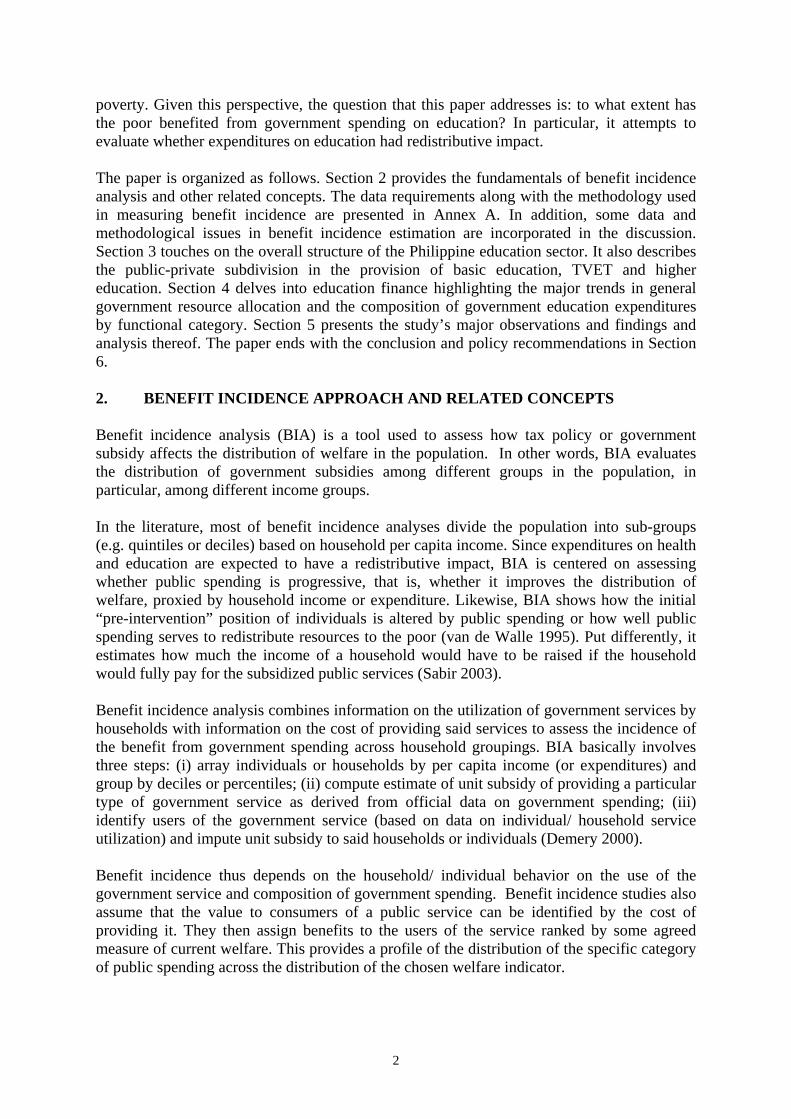
The paper is organized as follows. Section 2 provides the fundamentals of benefit incidence analysis and other related concepts. The data requirements along with the methodology used in measuring benefit incidence are presented in Annex A. In addition, some data and methodological issues in benefit incidence estimation are incorporated in the discussion. Section 3 touches on the overall structure of the Philippine education sector. It also describes the public-private subdivision in the provision of basic education, TVET and higher education. Section 4 delves into education finance highlighting the major trends in general government resource allocation and the composition of government education expenditures by functional category. Section 5 presents the study’s major observations and findings and analysis thereof. The paper ends with the conclusion and policy recommendations in Section 6. 2. BENEFIT INCIDENCE APPROACH AND RELATED CONCEPTS Benefit incidence analysis (BIA) is a tool used to assess how tax policy or government subsidy affects the distribution of welfare in the population. In other words, BIA evaluates the distribution of government subsidies among different groups in the population, in particular, among different income groups. In the literature, most of benefit incidence analyses divide the population into sub-groups (e.g. quintiles or deciles) based on household per capita income. Since expenditures on health and education are expected to have a redistributive impact, BIA is centered on assessing whether public spending is progressive, that is, whether it improves the distribution of welfare, proxied by household income or expenditure. Likewise, BIA shows how the initial “pre-intervention” position of individuals is altered by public spending or how well public spending serves to redistribute resources to the poor (van de Walle 1995). Put differently, it estimates how much the income of a household would have to be raised if the household would fully pay for the subsidized public services (Sabir 2003). Benefit incidence analysis combines information on the utilization of government services by households with information on the cost of providing said services to assess the incidence of the benefit from government spending across household groupings. BIA basically involves three steps: (i) array individuals or households by per capita income (or expenditures) and group by deciles or percentiles; (ii) compute estimate of unit subsidy of providing a particular type of government service as derived from official data on government spending; (iii) identify users of the government service (based on data on individual/ household service utilization) and impute unit subsidy to said households or individuals (Demery 2000). Benefit incidence thus depends on the household/ individual behavior on the use of the government service and composition of government spending. Benefit incidence studies also assume that the value to consumers of a public service can be identified by the cost of providing it. They then assign benefits to the users of the service ranked by some agreed measure of current welfare. This provides a profile of the distribution of the specific category of public spending across the distribution of the chosen welfare indicator.

3

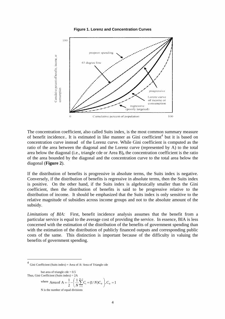
Benefit incidence analysis is better understood in relation to the concepts of targeting and progressivity of social spending. Targeting is a tool used to select eligible beneficiaries of any government intervention. In principle, it should concentrate the benefits of social assistance programs to the poorest segments of the population. All targeting mechanisms share a common objective: to correctly identify which households or individuals are poor and which are not. Targeting is a means of increasing the efficiency of the program by increasing the benefits that the poor can get with a fixed program budget (Coady, Grosh and Hoddinott 2004). Conversely, it is a means that will allow the government to reduce the budget requirement of the program while still delivering the same level of benefits to the poor. One way to assess the targeting of government subsidies is with reference to the graphical representation of the distribution of benefits, i.e., concentration curve or benefit concentration curve. A concentration curve is generated by plotting the cumulative distribution of “benefits” of public spending on the y-axis against the cumulative distribution of population sorted by per capita income on the x-axis. One can assess the progressivity or regressivity2 of a public subsidy by comparing the benefit concentration curve with the 45-degree diagonal and the Lorenz curve of income/ consumption.3 The diagonal indicates neutrality in the distribution of benefits. If the distribution of benefits lies along this line, the poorest 10 percent of the population gets 10 percent of the subsidy (could be income or consumption); poorest 20 percent account for 20 percent of the subsidy; and so on. Thus, the diagonal reflects perfect equality in the distribution of benefits and it is also referred to as perfect equality (PE) line. The distribution of benefits is said to be progressive if the lower income groups receive a larger share of the benefits from government spending than the richer income groups. For instance, if the concentration curve lies above the diagonal, then the poorest 10% of the population receives more than 10% of the benefits and the distribution of benefits is said to be progressive in absolute terms (Figure 1). Conversely, if the benefit concentration curve lies below the diagonal, then the poorest 10% of the population captures less than 10% of the benefits and the distribution of benefits is said to be regressive in absolute terms. On the other hand, a benefit concentration curve that lies above the Lorenz curve of income signifies progressivity of public subsidy relative to income. To wit, the benefits share of the poorest 10% of the population is larger than its income share. Thus, if the benefits from the government service is converted to its income equivalent, the post-subsidy distribution of income-cum-benefit would be more equitable than the original distribution of income if the benefit concentration curve lies above the Lorenz curve of income. Conversely, a concentration curve that lies below the Lorenz curve of income distribution suggests transfers that are more regressively distributed than income.

2 Progressivity implies a preference for lower income groups while regressivity implies a more favorable treatment of higher income groups. 3 Lorenz curve is a graphical depiction of the cumulative distribution of income on the y-axis against the cumulative distribution of population on the x-axis.

4

Figure 1. Lorenz and Concentration Curves

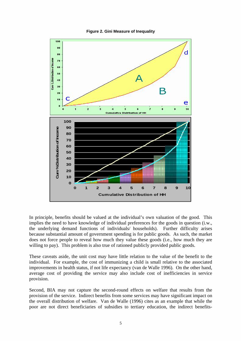
The concentration coefficient, also called Suits index, is the most common summary measure of benefit incidence.. It is estimated in like manner as Gini coefficient4 but it is based on concentration curve instead of the Lorenz curve. While Gini coefficient is computed as the ratio of the area between the diagonal and the Lorenz curve (represented by A) to the total area below the diagonal (i.e., triangle cde or Area B), the concentration coefficient is the ratio of the area bounded by the diagonal and the concentration curve to the total area below the diagonal (Figure 2). If the distribution of benefits is progressive in absolute terms, the Suits index is negative. Conversely, if the distribution of benefits is regressive in absolute terms, then the Suits index is positive. On the other hand, if the Suits index is algebraically smaller than the Gini coefficient, then the distribution of benefits is said to be progressive relative to the distribution of income. It should be emphasized that the Suits index is only sensitive to the relative magnitude of subsidies across income groups and not to the absolute amount of the subsidy. Limitations of BIA: First, benefit incidence analysis assumes that the benefit from a particular service is equal to the average cost of providing the service. In essence, BIA is less concerned with the estimation of the distribution of the benefits of government spending than with the estimation of the distribution of publicly financed outputs and corresponding public costs of the same. This distinction is important because of the difficulty in valuing the benefits of government spending.

4 Gini Coefficient (Suits index) = Area of A/ Area of Triangle cde

but area of triangle cde = 0.5 Thus, Gini Coefficient (Suits index) = 2A

where 1 , )/1(121A of Area

1

1

=⎟⎠

⎞⎜⎝

⎛+−= ∑

−

=NN

N

ii CCNC

N

N is the number of equal divisions

5

Figure 2. Gini Measure of Inequality

01020

3040506070

8090

100

0 1 2 3 4 5 6 7 8 9 10

Cumulative Distribution of HH

Cum

% D

istr

ibut

ion

of In

com

e

In principle, benefits should be valued at the individual’s own valuation of the good. This implies the need to have knowledge of individual preferences for the goods in question (i.w., the underlying demand functions of individuals/ households). Further difficulty arises because substantial amount of government spending is for public goods. As such, the market does not force people to reveal how much they value these goods (i.e., how much they are willing to pay). This problem is also true of rationed publicly provided public goods. These caveats aside, the unit cost may have little relation to the value of the benefit to the individual. For example, the cost of immunizing a child is small relative to the associated improvements in health status, if not life expectancy (van de Walle 1996). On the other hand, average cost of providing the service may also include cost of inefficiencies in service provision.

Second, BIA may not capture the second-round effects on welfare that results from the provision of the service. Indirect benefits from some services may have significant impact on the overall distribution of welfare. Van de Walle (1996) cites as an example that while the poor are not direct beneficiaries of subsidies to tertiary education, the indirect benefits-

6

transmitted through good governance and the overall improvement in capability of the government bureaucracy may be of significance to the well-being and livelihood of the poor. Third, benefit incidence analysis generally refer to the distribution of average benefits. Oftentimes, however, the marginal benefits distribution are just as important. Again, van de Walle (1996) notes that a seemingly beneficial expansion in the primary school budget may be buying better quality schools in which the relatively better-off are enrolled rather than more public schools for the under-served poor. Fourth, benefit incidence analysis does not take into account the long-run impact of government spending on beneficiaries. Rather, it simply focuses on how effective government spending is in transferring current income to the poorest households (Demery 2000). Data sources. Government spending data on an obligation basis is obtained from the Budget of Expenditures and Sources of Financing (DBM various years) for the national government and from the Annual Financial Report (AFR) for Local Government Units of the Commission on Audit (COA). Enrollment data for the different income groups in different levels of education is obtained from the 1998 and 1999 Annual Poverty Indicators Survey. 3. OVERALL STRUCTURE OF THE PHILIPPINE EDUCATION SECTOR The Philippine Constitution of 1987 mandates the establishment and maintenance of a system of free public education at the elementary and secondary level. It also ordains that the state should assign the highest budgetary priority to education. The Philippine educational system covers both formal and non-formal education. Formal education is a sequential academic schooling with three levels: (1) basic education, (2) technical/vocational education and training; and (3) higher education. Completion of each level is required to get into the next. Parents with kids aged 3-5 have the option to send them to pre-school for kindergarten schooling and other preparatory courses before they proceed to grade one at age 6. Pre-school education is usually offered in private schools although some public schools do have kindergarten classes. In comparison, non-formal education includes any organized and systematic learning conducted largely outside school premises. It addresses the needs of those who are unable to participate in formal education primarily due to poverty. Non-formal education caters to out-of-school youth or adult illiterates. To date, non-formal education in the country focuses on family life skills, including health, nutrition, childcare, household management, and family planning; vocational skills; functional literacy; and livelihood skills.5

5 http://www.ilo.org/public/english/employment/skills/hrdr/init/phi_12.htm

7

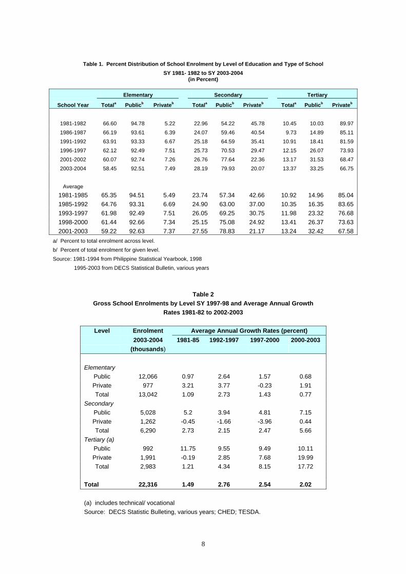
Basic education involves compulsory six years of elementary schooling in public schools and 4 years of secondary schooling. Elementary education is provided free of charge by the state and is compulsory, in principle. In contrast, secondary education is considered voluntary but the 1987 Constitution likewise mandates the state to provide it for free. While basic education is typically provided in stand-alone schools, some elementary and secondary schools are attached to universities and colleges partly due to these facts: (1) many higher education institutions were actually upgraded basic education institutions and (2) teacher training institutions maintain their own ‘laboratory’ schools (Maglen and Manasan 1999). It should be noted, however, that since 1998 SUCs are only allowed to maintain elementary and secondary schools if they actually offer teacher training programs and even then, enrolment in their ‘laboratory’ schools is limited to 500. After completion of basic education, students can go for technical/vocational education and training (TVET) or pursue higher education depending on their academic and financial capabilities. TVET level provides pre-employment preparation in middle level technician and craft skills. At the formal post-secondary level, TVET programs may have a duration of up to 3 years and may lead to certificate and diploma qualifications. Further, technical and vocational education programs are conducted at both the secondary and post-secondary level. Prior to 1995, technical and vocational high schools were operated by the former Bureau of Technical and Vocational Education (BTVE) under the DECS. Since 1994, 207 of these schools were transferred to the Technical Education and Skills Development Authority (TESDA).6 On the other hand, higher education is composed of three levels namely collegiate/tertiary, master’s and doctorate in various disciplines. Collegiate or tertiary education may take 4 or more years and leads to bachelor’s degree. By and large, higher education is offered in colleges and universities that offer, exclusively or primarily, the usual range of undergraduate and postgraduate programs. Elementary education is largely provided by the public sector. Thus, the government is the dominant provider of places at the elementary level, accounting for about 93% of total elementary level enrolment throughout 1981-2004 (Table 1). In contrast, the public-private subdivision in the provision of secondary education is traditionally more even. However, the share of the private sector in total secondary enrolment has been eroded over time, contracting from 46% in SY 1981-1982 to 30% in SY 1996-1997 to 20% in SY 2003-2004. This came about as enrolment in public schools expanded by 3.9% yearly on the average in 1992-1997 and 6.0% in 1997-2003 while that in private schools contracted by 1.8% per annum in 1992-2003 (Table 2). The decline in the number of students enrolled in private secondary schools was dramatic (4.0%) in 1996-2000. This downward trend in the number of students in private secondary schools has persisted in 2003-2004 but in a more subdued fashion. In toto, public schools appear to have crowded out private schools the 1987 Constitution’s mandate for the state to provide free secondary education.

6 In 1998, however, 163 of these schools were transferred back to DECS after it was assessed that their programs were general in nature rather than technical and vocational.

8

Table 1. Percent Distribution of School Enrolment by Level of Education and Type of School

SY 1981- 1982 to SY 2003-2004 (in Percent)

Elementary Secondary Tertiary

School Year Totala Publicb Privateb Totala Publicb Privateb Totala Publicb Privateb

1981-1982 66.60 94.78 5.22 22.96 54.22 45.78 10.45 10.03 89.97 1986-1987 66.19 93.61 6.39 24.07 59.46 40.54 9.73 14.89 85.11 1991-1992 63.91 93.33 6.67 25.18 64.59 35.41 10.91 18.41 81.59 1996-1997 62.12 92.49 7.51 25.73 70.53 29.47 12.15 26.07 73.93 2001-2002 60.07 92.74 7.26 26.76 77.64 22.36 13.17 31.53 68.47 2003-2004 58.45 92.51 7.49 28.19 79.93 20.07 13.37 33.25 66.75

Average

1981-1985 65.35 94.51 5.49 23.74 57.34 42.66 10.92 14.96 85.04 1985-1992 64.76 93.31 6.69 24.90 63.00 37.00 10.35 16.35 83.65 1993-1997 61.98 92.49 7.51 26.05 69.25 30.75 11.98 23.32 76.68 1998-2000 61.44 92.66 7.34 25.15 75.08 24.92 13.41 26.37 73.63 2001-2003 59.22 92.63 7.37 27.55 78.83 21.17 13.24 32.42 67.58

a/ Percent to total enrolment across level. b/ Percent of total enrolment for given level. Source: 1981-1994 from Philippine Statistical Yearbook, 1998 1995-2003 from DECS Statistical Bulletin, various years

Table 2 Gross School Enrolments by Level SY 1997-98 and Average Annual Growth

Rates 1981-82 to 2002-2003

Level Enrolment Average Annual Growth Rates (percent) 2003-2004 1981-85 1992-1997 1997-2000 2000-2003 (thousands) Elementary

Public 12,066 0.97 2.64 1.57 0.68 Private 977 3.21 3.77 -0.23 1.91 Total 13,042 1.09 2.73 1.43 0.77

Secondary Public 5,028 5.2 3.94 4.81 7.15 Private 1,262 -0.45 -1.66 -3.96 0.44 Total 6,290 2.73 2.15 2.47 5.66

Tertiary (a) Public 992 11.75 9.55 9.49 10.11 Private 1,991 -0.19 2.85 7.68 19.99 Total 2,983 1.21 4.34 8.15 17.72

Total 22,316 1.49 2.76 2.54 2.02 (a) includes technical/ vocational Source: DECS Statistic Bulleting, various years; CHED; TESDA.

9

While the public sector remains to be a relatively small player at the tertiary level, government institutions have increasingly become more important given the dramatic rise in the number of SUCs in the last 20 years. Thus, the share of the public sector in total tertiary enrolment rose from 10% in school year SY 1981-1982 to 26% in SY 1996-1997 and 33% in SY 2003-2004. This came about as the number of students in public tertiary institutions rose at a rate that is more than thrice as fast (8.9% yearly) as that in private institutions (2.4% annually) in 1997-2003. Prior to 1994, the Department of Education Culture and Sports (DECS), now the Department of Basic Education (DepEd), had the sole responsibility for policy formulation, planning, budgeting, program implementation and coordination of all levels of formal and non-formal education in the Philippines. It also supervised all education institutions in both the public and the private sectors. When the “trifocalization” policy took effect in 1994/1995, the oversight for the education sector is provided by three distinct bodies: the Department of Education (DepEd) for basic education; the Technical Education and Skills Development Authority (TESDA) for technical and vocational education and training; and the Commission on Higher Education (CHED) for higher education. All three agencies are in charge of policy formulation, planning, programming, coordination, supervision of public and private institutions, and standard setting in each of their respective sub-sectors. In addition, the DepEd and the TESDA run their own schools and training centers. Moreover, as part of the devolution of the construction and maintenance of local infrastructure under the Local Government Code of 1991, the responsibility for the construction and maintenance of public elementary and secondary schools is assigned principally to municipal and city governments. However, the central government through the DepEd continues to be in charge of the operation of public elementary and secondary schools.7 In contrast, the CHED has no direct hand in the day-to-day operation of any state university or college (SUC) although CHED commissioners sit on the board of the SUCs. The CHED is composed of full-time commissioners, all appointed by the President of the Philippines and is attached to the Office of the President. On the other hand, the TESDA took over the functions and responsibilities of the former National Manpower and Youth Council (NMYC) and the former Office of Apprenticeship (OA) and the former Bureau of Technical and Vocational Education (BTVE) of the old DECS. Organizationally, the TESDA, like the NMYC and OA before it, is attached to the Department of Labor and Employment (DOLE). The 1998 Philippine Education Sector Study (PESS) and the Presidential Commission on Educational Reform (PCER) point out that a tripartite form of sector management has made it difficult to formulate sectoral policy and to decide on rational allocation of resources across the different sub-sectors. The PESS, in particular, pointed out that there is a need to avoid areas of duplication and overlap and to address regulatory gaps that have emerged since the implementation of trifocalization.

7 The law creating the Department of Education provides that the new DepEd sheds off the responsibility for culture and sports that old Department of Education Culture and Sports (DECS) had.

10

In order to improve overall sector governance, the PCER recommended the creation of a National Coordinating Council for Education (NCCE) that will coordinate policies and plans. On the other hand, the PESS pointed out that while a body like the NCCE can effectively address issues of coordination and functional overlap, the NCCE, being a “fraternity of educators,” is not likely to have much success in making unbiased judgments about intra-sectoral allocation of resources. The PESS noted that the determination of intersectoral and intra-sectoral priorities is a decision that is best taken as part of the government’s overall budget-setting process at the level of the DBCC. The NCCE was in fact formally established in 2000 with the issuance of Executive Order 273 by then President Joseph Estrada. To date, however, it is not fully operational. While the council has started to meet and the rotating chairmanship has been held first by the DepEd Secretary and now by the CHED Chairman, the Technical Secretariat that was supposed to provide staff support to the council has not been constituted because of the lack of funding. Very recently, the President was reported to have delegated the Secretary of the DepEd oversight function over the CHED, thereby raising questions on relationship between these two agencies. In the meantime, there appears no forum where intra-sectoral priorities are effectively discussed. For instance, there is widespread agreement that the basic education cycle, being limited to 10 years, is too short. The DepEd has responded by developing a bridge program that essentially adds an additional year to the secondary level. On the other hand, the CHED proposes to introduce a pre-baccalaureate year. However, a systematic evaluation of these alternative options has not been done to date. 4. EDUCATION FINANCE The PESS showed that public plus private education spending rose markedly between 1986 and 1997, with the largest increase coming from private spending. In 1997-2003, the opposite trend is observable. The total amount of funds available to the education sector from all sources declined from 6.2% of GNP in 1997 to 5.7% in 2000 and 5.0% in 2003 (Figure 3). This movement is largely driven by the contraction of government spending on the sector.8 Household spending was partly able to compensate for some of this decline in 2000. However, in 2003, the reduction in government spending is further reinforced by the decrease in private spending. The fall in both government and private financing of the education is a cause for concern given the rapid growth of the population and the resulting pressures that this puts on demand for education places. 4.1. Major Expenditure Trends in General Government Resource Allocation

In response to shortfalls in government revenues, large fiscal deficits and ballooning public debt levels, the government implemented fiscal adjustment measures that mostly affected the expenditure side of the budget in 1998-2005. However, fiscal consolidation has not been kind to the education sector. 8 It should be emphasized that the estimates of household education spending found in this paper are not directly comparable to those in PESS. The figures in this paper are the unadjusted numbers obtained from the Family Income and Expenditure Survey (FIES). Those from the PESS are partly based on a FAPE survey and on partly on the FIES. However, the levels are perhaps less important than the changes in the levels.

11

Figure 3. Total Education Finance(Percent to GNP)

0.01.02.03.04.05.06.07.0

1997 2000 2003

Year

Per

cent

to G

NP

Household Government

Central government. Central government spending on all the major sectors (except debt service) contracted relative of GDP in 1999-2005.9 This occurred as rising interest payments and, to a lesser extent, transfers to LGUs put the squeeze on non-mandatory expenditures of the central government. The economic services sectors bore the brunt of this adjustment. In contrast, the social services sectors were given greater priority over other sectors and their share in total central government spending net of debt service and transfers to LGUs (i.e., the IRA) expanded from an average of 35.5% in 1992-1998 to 39.7% in 1999-2000. Although it went down to 39.4% in 2001-2005, it is still higher than the average in the 1992-1998 sub-period (Figure 4).

Figure 4. Percent Distribution of National Government ExpendituresRelative to Total Expenditure Net of Debt Service & IRA, 1986-2005

1992-19981986-1991

1999-2000

PublicService17.04%

SocialServices30.26%

NationalDefense11.29%

EconomicServices37.35%


PublicService21.16%





PublicService20.74%


2001-2005NationalDefense9.56%


PublicService21.39%


9 Although the IRA of LGUs rose somewhat in 1998-2000, it remained fairly constant in 2001-2003.

12

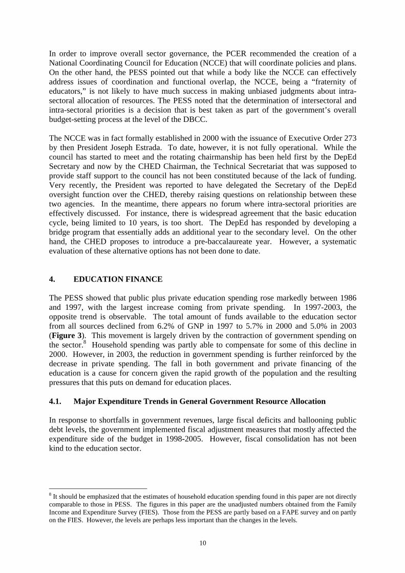
However, the budget pie has grown smaller and central government spending on all social services combined declined from a peak of 5.5% of GDP in 1998 to 3.2% in 2005. Likewise, education spending of the central government was adversely affected by the fiscal contraction as central government expenditures on the sector shrank from 4.0% of GDP in 1998 to 2.5% of GDP in 2005 (Figure 5).

Figure 5. National Government Expenditures as Percent of GDP, 1987-2005

0.00

5.00

10.00

15.00

20.00

25.00

1987 1988 1989 1990 1991 1992 1993 1994 1995 1996 1997 1998 1999 2000 2001 2002 2003 2004 2005

Year

Perc

ent

Grand Total Debt Service (Interests) GT-DS-IRA Education IRA GT-DS

Consequently, by 2003 central government spending on education in the Philippines (2.8% of GNP) has lagged even farther behind the spending level of its Asian neighbors like Malaysia (7.9%), Thailand (4.1%), and Singapore (4.3%) (Table 3).

Table 3. Education Expenditures of Central Government, 1985-2003 Percent of GNP 1985 1990 1995 2000 2003 Indonesia .. 1.04 - 1.01 1.28 Malaysia 6.61 5.45 5.00 6.38 7.91 Philippines 1.35 2.90 3.15 3.28 2.77 Singapore a/ 4.40 3.01 2.98 3.98 4.23 Thailand 3.79 3.59 3.59 4.55 4.13 Percent Share to Total Expenditures 1995 2000 2003 Indonesia - 5.37 8.45 Malaysia 20.94 23.70 25.51 Philippines 16.57 17.12 17.92 Singapore a/ 18.89 21.03 19.44 Thailand 23.03 25.83 24.19 a/ 2001 data Source: Asian Development Bank Key Indicators for 1995-2003 UNESCO for 1985 and 1990

13

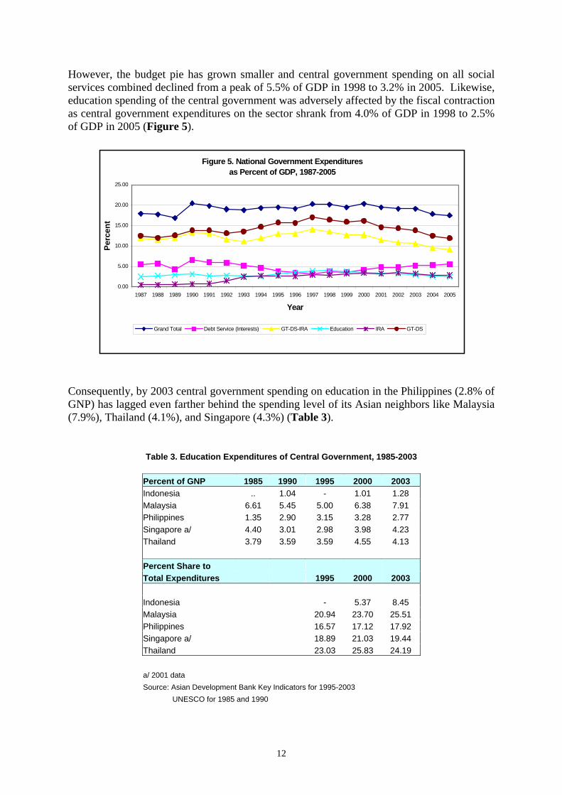
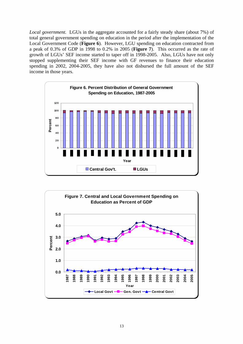
Local government. LGUs in the aggregate accounted for a fairly steady share (about 7%) of total general government spending on education in the period after the implementation of the Local Government Code (Figure 6). However, LGU spending on education contracted from a peak of 0.3% of GDP in 1998 to 0.2% in 2005 (Figure 7). This occurred as the rate of growth of LGUs’ SEF income started to taper off in 1998-2005. Also, LGUs have not only stopped supplementing their SEF income with GF revenues to finance their education spending in 2002, 2004-2005, they have also not disbursed the full amount of the SEF income in those years.

Figure 6. Percent Distribution of General Government Spending on Education, 1987-2005

0

2 0

4 0

6 0

8 0

10 0

12 0

Year

Perc

ent

Central Gov't. LGUs

Figure 7. Central and Local Government Spending on Education as Percent of GDP

0.0

1.0

2.0

3.0

4.0

5.0

1987

1988

1989

1990

1991

1992

1993

1994

1995

1996

1997

1998

1999

2000

2001

2002

2003

2004

2005

Year

Perc

ent

Local Govt Gen. Govt Central Govt

14

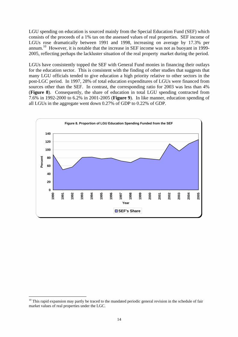
LGU spending on education is sourced mainly from the Special Education Fund (SEF) which consists of the proceeds of a 1% tax on the assessed values of real properties. SEF income of LGUs rose dramatically between 1991 and 1998, increasing on average by 17.3% per annum.10 However, it is notable that the increase in SEF income was not as buoyant in 1999-2005, reflecting perhaps the lackluster situation of the real property market during the period. LGUs have consistently topped the SEF with General Fund monies in financing their outlays for the education sector. This is consistent with the finding of other studies that suggests that many LGU officials tended to give education a high priority relative to other sectors in the post-LGC period. In 1997, 28% of total education expenditures of LGUs were financed from sources other than the SEF. In contrast, the corresponding ratio for 2003 was less than 4% (Figure 8). Consequently, the share of education in total LGU spending contracted from 7.6% in 1992-2000 to 6.2% in 2001-2005 (Figure 9). In like manner, education spending of all LGUs in the aggregate went down 0.27% of GDP to 0.22% of GDP.

Figure 8. Proportion of LGU Education Spending Funded from the SEF

0

20

40

60

80

100

120

140

1990

1991

1992

1993

1994

1995

1996

1997

1998

1999

2000

2001

2002

2003

2004

2005

Year

Perc

ent

SEF's Share

10 This rapid expansion may partly be traced to the mandated periodic general revision in the schedule of fair market values of real properties under the LGC.

15

Figure 9. Share of Education to Total LGU Budget

0.01.02.03.04.05.06.07.08.09.0

10.0

1990

1991

1992

1993

1994

1995

1996

1997

1998

1999

2000

2001

2002

2003

2004

2005

Year

Perc

ent

Share of Education to Total LGU Budget

Given the relative size of central and local government spending on education, the movement in general government spending largely mirrored what is happening at the central government level. Total general government expenditure on education started to slide in 1999 when expressed relative to either GDP or total general government spending. This downward trend persists up to the present. Thus, total general government outlays on education slid from 4.3% of GDP in 1998 to 2.6% of GDP in 2005 (Figure 7). At the same time, the education sector’s share in aggregate general government expenditure contracted from 20.5% in 1998 to 14.9% in 2005 (Figure 10).

Figure 10. Central and Local Government Expenditure on Education as Percent of Total Budget

0.0

5.0

10.0

15.0

20.0

25.0

1987

1988

1989

1990

1991

1992

1993

1994

1995

1996

1997

1998

1999

2000

2001

2002

2003

2004

2005

Year

Per

cent

Gen. Govt Central Govt Local Govt

16

4.2. Composition of Government Education Expenditures by Functional Category

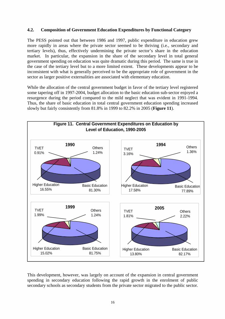
The PESS pointed out that between 1986 and 1997, public expenditure in education grew more rapidly in areas where the private sector seemed to be thriving (i.e., secondary and tertiary levels), thus, effectively undermining the private sector’s share in the education market. In particular, the expansion in the share of the secondary level in total general government spending on education was quite dramatic during this period. The same is true in the case of the tertiary level but to a more limited extent. These developments appear to be inconsistent with what is generally perceived to be the appropriate role of government in the sector as larger positive externalities are associated with elementary education. While the allocation of the central government budget in favor of the tertiary level registered some tapering off in 1997-2004, budget allocation to the basic education sub-sector enjoyed a resurgence during the period compared to the mild neglect that was evident in 1991-1994. Thus, the share of basic education in total central government education spending increased slowly but fairly consistently from 81.8% in 1999 to 82.2% in 2005 (Figure 11).

Figure 11. Central Government Expenditures on Education byLevel of Education, 1990-2005

1990 1994

1999

Basic Education81.30%

TVET0.91%

Higher Education16.55%


TVET3.16%




TVET1.99%

Others1.24%

Others1.24%

Others1.36%

2005



TVET1.81%

Others2.22%

This development, however, was largely on account of the expansion in central government spending in secondary education following the rapid growth in the enrolment of public secondary schools as secondary students from the private sector migrated to the public sector.

17

Thus, the share of the secondary level in total central government spending on education rose 19.3% in 1996 to 21.4% in 1999 to 23.1% in 2003 and 24.4% in 2005. In contrast, the share of the elementary level in total central government education expenditure was fairly stable at about 60% in 1997-2002 but went down to 58.7% in 2003 and 57.4% in 2005. The expansion in the share of secondary education in total central government spending on education in 1997-2004 came at the expense of both higher education and TVET. Even with the relatively more comfortable overall fiscal position of the national government in the mid-1990s, the budget share of higher education started to contract since 1997 despite the big increase in the number of SUCs in the late 1990s. This came about as the Department of Budget and Management (DBM) used the budget process to help rationalize the higher education sub-sector.11 Thus, the share of higher education in the total education budget of the central government is now down to 13.8% in 2005 from a high of 17.6% in 1994. In contrast, higher education and TVET captured an increasing portion of LGUs’ education expenditure. Thus, the share of higher education in total LGU spending on education expanded dramatically from less than 1% in 1997 to 7% in 2005 following the creation of LGU funded universities and colleges during the period (Figure 12).12 In like manner, the share of TVET in total LGU spending on education almost tripled from 1% in 1997 to 2.7% in 2003. This reallocation came at the expense of the basic education sub-sector as its budget share dipped from 82% of total aggregate LGU spending on education in 1997 to 70% in 2005.

Figure 12. Composition of All LGUs Expenditure on Education, 1997 and 2005

1997

Basic Educ.81.92%

Others16.31%

Higher Educ.0.68%

Manpower Dev't.1.09%

2005

Basic Educ.70.17%

Others21.03%

Higher Educ.6.09%

Manpower Dev't.2.71%

On the whole, the composition of general government spending on the education sector is largely a reflection of the developments at the central government level. Thus, after contracting to an average of 78% in 1991-1994, the share of the basic education sub-sector in the total education budget of the general government recovered to an average of 82% in 2001-2005. This occurred as the share of both higher education and technical /vocational education and training in the budget dipped to 13.4% and 1.9%, respectively, in 2001-2005 from 16.2% and 3.4%, in 1991-1994 (Figure 13).

11 Since 2000, the DBM has gradually reduced the MOOE item in the SUCs’ budgets. 12 There are 44 LUCs as of end of 2003.

18

Figure 13. General Government Expenditures on Education by

Level of Education, 1991-2005

1991-1994 2001-2005



TVET3.38%


TVET1.88%


Others3.13%

Others2.09%

5. ANALYSIS OF BENEFIT INCIDENCE OF GOVERNMENT EXPENDITURE

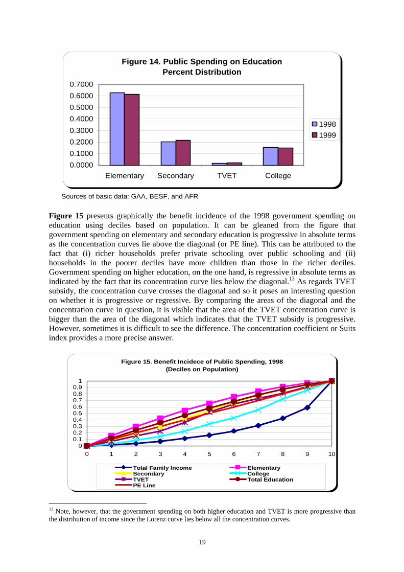
ON EDUCATION National level estimates. The total budget for public education was almost PhP 105B in 1998. More than half, i.e., 62.7 percent, of the budget was allocated to elementary education and 20.3 percent to secondary education. The combined share of elementary and secondary education to the total budget shows that basic education was given the highest priority in government spending on education. This also holds true for 1999 wherein the share of elementary and secondary education to total budget (PhP 109B) was 61.6 percent and 21.5 percent, respectively. Although the budget share for elementary education went down, the increase in the budget share for secondary education kept the combined share at about 83 percent leaving a meager amount for TVET and college education (Figure 14). This spending pattern implies that government tends to favor the poor if one is to take the common belief that basic services (e.g. basic education) matter more to the poor than do other government services. A closer look at the numbers provides more insightful information as to which income group benefits most in public spending in each education level.

19

Sources of basic data: GAA, BESF, and AFR

Figure 14. Public Spending on Education Percent Distribution

0.00000.10000.20000.30000.40000.50000.60000.7000

Elementary Secondary TVET College

19981999

Figure 15 presents graphically the benefit incidence of the 1998 government spending on education using deciles based on population. It can be gleaned from the figure that government spending on elementary and secondary education is progressive in absolute terms as the concentration curves lie above the diagonal (or PE line). This can be attributed to the fact that (i) richer households prefer private schooling over public schooling and (ii) households in the poorer deciles have more children than those in the richer deciles. Government spending on higher education, on the one hand, is regressive in absolute terms as indicated by the fact that its concentration curve lies below the diagonal.13 As regards TVET subsidy, the concentration curve crosses the diagonal and so it poses an interesting question on whether it is progressive or regressive. By comparing the areas of the diagonal and the concentration curve in question, it is visible that the area of the TVET concentration curve is bigger than the area of the diagonal which indicates that the TVET subsidy is progressive. However, sometimes it is difficult to see the difference. The concentration coefficient or Suits index provides a more precise answer.

Figure 15. Benefit Incidece of Public Spending, 1998 (Deciles on Population)

00.10.20.30.40.50.60.70.80.9

1

0 1 2 3 4 5 6 7 8 9 10

Total Family Income ElementarySecondary CollegeTVET Total EducationPE Line

13 Note, however, that the government spending on both higher education and TVET is more progressive than the distribution of income since the Lorenz curve lies below all the concentration curves.

20

Table 4 presents the cumulative distribution of income and education subsidy with the corresponding Suits index. Government spending on elementary and secondary education in 1998 are found to be progressive. Although government subsidies to college education and TVET are regressive, the Suits index for total government spending on education signals progressivity.

Table 4. Cumulative Distribution of Income and Education Subsidy, 1998 and 1999 (%)

Using deciles based on Population, 1998Deciles Income Elementary Secondary College TVET Total

1 1.52 15.39 8.39 3.36 6.86 11.972 3.97 29.59 19.22 8.73 15.75 24.043 7.21 42.64 30.27 15.03 22.27 35.544 11.32 54.54 41.92 22.35 36.11 46.715 16.47 65.32 54.56 33.41 51.92 57.986 22.98 75.40 66.35 42.77 64.31 68.337 31.35 84.01 77.88 55.62 72.79 78.198 42.51 91.10 87.26 72.36 81.21 87.269 58.68 96.81 95.22 85.85 91.25 94.7010 100.00 100.00 100.00 100.00 100.00 100.00

Suits Index 0.5080 -0.2096 -0.0621 0.2210 0.0151 -0.1094

Using deciles based on Population, 1999Deciles Income Elementary Secondary College TVET Total

1 1.58 15.16 8.35 2.43 3.88 11.582 4.12 29.39 18.90 7.06 10.49 23.443 7.45 42.56 30.42 13.34 15.24 35.064 11.64 54.27 42.04 21.05 23.63 46.095 16.87 65.00 54.24 32.19 31.95 57.156 23.45 75.05 65.60 43.19 54.38 67.877 31.92 83.61 76.93 55.93 68.31 77.758 43.30 91.02 87.30 68.66 79.05 86.669 59.68 96.69 95.40 86.55 91.86 94.8010 100.00 100.00 100.00 100.00 100.00 100.00

Suits Index 0.5000 -0.2055 -0.0583 0.2392 0.1424 -0.1008

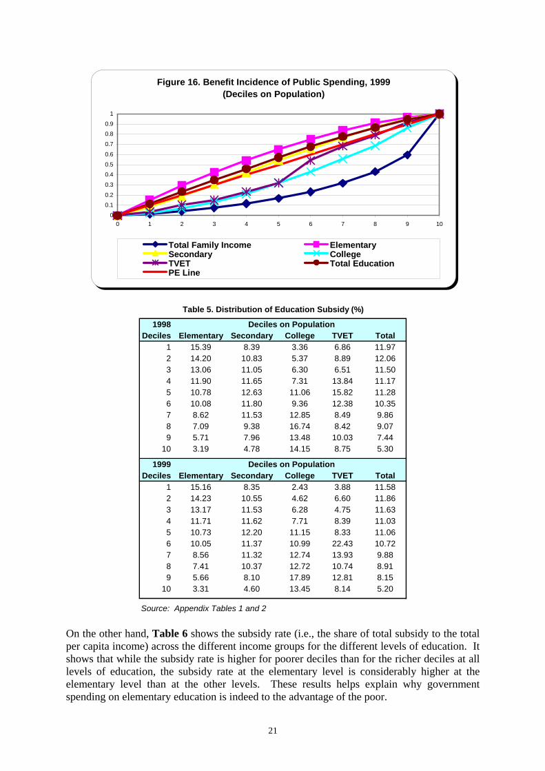
On the one hand, Figure 16 presents the benefit concentration curves of public spending on education in 1999. Looking at the two graphs, the elementary and secondary concentration curves dominate the diagonal and thus, subsidies in elementary and secondary education are progressive. On the contrary, TVET and college subsidies are regressive as their concentration curves are lying below the diagonal. Again, the estimated Suits index speaks for it.

Table 5 shows the distribution of education subsidy across the different deciles for the different levels of education. It shows that while the poorer deciles capture a bigger share of the government spending in the elementary and secondary levels the opposite is true for government spending on higher education. To wit, the poorest 10% of the population capture 15% of aggregate government spending on elementary education while the richest decile only gets a 3% share. In contrast, the poorest 10% of the population receives 3% of aggregate government spending on college education while the richest 10% gets a 14% share.

21

Figure 16. Benefit Incidence of Public Spending, 1999 (Deciles on Population)

0

0.1

0.2

0.3

0.4

0.5

0.6

0.7

0.8

0.9

1

0 1 2 3 4 5 6 7 8 9 10

Total Family Income ElementarySecondary CollegeTVET Total EducationPE Line

Table 5. Distribution of Education Subsidy (%)

1998 Deciles on PopulationDeciles Elementary Secondary College TVET Total

1 15.39 8.39 3.36 6.86 11.972 14.20 10.83 5.37 8.89 12.063 13.06 11.05 6.30 6.51 11.504 11.90 11.65 7.31 13.84 11.175 10.78 12.63 11.06 15.82 11.286 10.08 11.80 9.36 12.38 10.357 8.62 11.53 12.85 8.49 9.868 7.09 9.38 16.74 8.42 9.079 5.71 7.96 13.48 10.03 7.44

10 3.19 4.78 14.15 8.75 5.30

1999 Deciles on PopulationDeciles Elementary Secondary College TVET Total

1 15.16 8.35 2.43 3.88 11.582 14.23 10.55 4.62 6.60 11.863 13.17 11.53 6.28 4.75 11.634 11.71 11.62 7.71 8.39 11.035 10.73 12.20 11.15 8.33 11.066 10.05 11.37 10.99 22.43 10.727 8.56 11.32 12.74 13.93 9.888 7.41 10.37 12.72 10.74 8.919 5.66 8.10 17.89 12.81 8.15

10 3.31 4.60 13.45 8.14 5.20

Source: Appendix Tables 1 and 2 On the other hand, Table 6 shows the subsidy rate (i.e., the share of total subsidy to the total per capita income) across the different income groups for the different levels of education. It shows that while the subsidy rate is higher for poorer deciles than for the richer deciles at all levels of education, the subsidy rate at the elementary level is considerably higher at the elementary level than at the other levels. These results helps explain why government spending on elementary education is indeed to the advantage of the poor.

22

Table 6. Subsidy Rate by Decile (%)1998 Deciles based on Population

Decile Elementary Secondary College TVET Total1 39.76 7.01 2.15 0.44 49.362 22.66 5.59 2.12 0.35 30.723 15.76 4.31 1.88 0.20 22.154 11.33 3.59 1.72 0.33 16.975 8.19 3.10 2.08 0.30 13.676 6.06 2.29 1.39 0.18 9.937 4.03 1.74 1.49 0.10 7.368 2.49 1.06 1.45 0.07 5.089 1.38 0.62 0.81 0.06 2.87

10 0.30 0.15 0.33 0.02 0.801999 Deciles based on Population

Decile Elementary Secondary College TVET Total1 36.70 7.05 1.42 0.30 45.482 21.49 5.56 1.69 0.32 29.053 15.14 4.62 1.74 0.17 21.674 10.67 3.70 1.70 0.24 16.315 7.86 3.12 1.97 0.20 13.146 5.85 2.31 1.55 0.42 10.127 3.87 1.78 1.39 0.20 7.248 2.49 1.22 1.03 0.12 4.869 1.32 0.66 1.01 0.10 3.09

10 0.31 0.15 0.31 0.02 0.80

Source: Appendix Tables 1 and 2

Furthermore, assuming that the 1999 distribution of benefit incidence remains unchanged until 2005, results of analysis of education subsidy for the succeeding years, 2000 up to 2005 also imply the progressivity of elementary and secondary subsidy as well as the regressivity of TVET and college subsidy. Table 7 presents the computed Suits index for the education sector if one assumes the enrollment rates across income deciles remain unchanged for the different levels of education in 1999-2005 but actual changes in the composition of government spending in the sector are taken into consideration. While the progressivity of the total education is evident in all years, it declined, albeit slowly, in 2001-2004. This is associated with the decline in the share of elementary education in total education spending from 1999 onwards as the share of secondary education increased.

Table 7. Suits Index for Total Education Spending

1998-2005

1998 -0.109441999 -0.100802000 -0.100572001 -0.105452002 -0.105442003 -0.104312004 -0.103062005 -0.10098

23

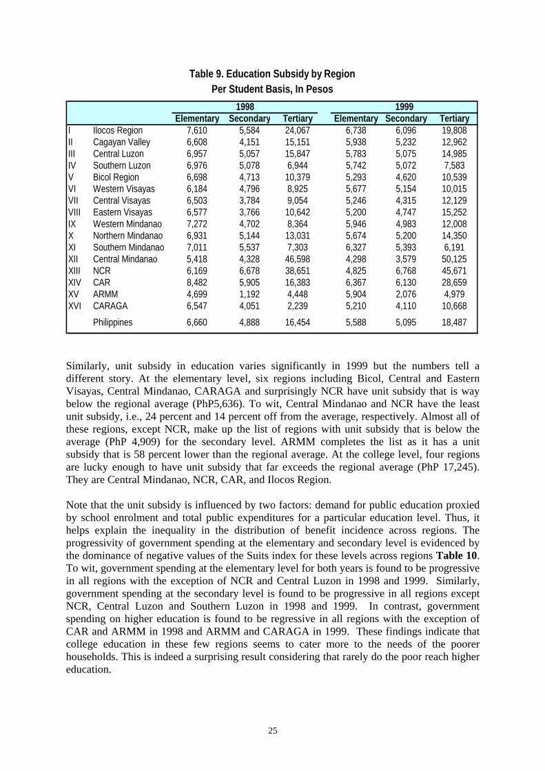
Regional level estimates Table 8 shows the distribution of education subsidy across regions. Evidently, there is a wide disparity in the share of the different regions in government education spending. It can be gleaned from the table that richer regions such as NCR, Southern and Central Luzon have higher share in the education budget as opposed to the poorer regions specifically ARMM, CARAGA and CAR. This is consistent with the common observation that services in urban areas usually attract higher subsidies compared to those of rural areas. In both years, the National Capital Region (NCR) got the biggest share in both secondary and college subsidy relative to the rest of the regions. In 1998, the NCR’s budget for secondary and college education accounted for about 15% and 38% of the total sectoral budget, respectively. The shares declined by 1 percentage point in 1999 but NCR remained as top beneficiary in both levels. In comparison, ARMM and CARAGA had the smallest share in government secondary and college spending, respectively. ARMM’s budget share for secondary education is around 1% for both years while CARAGA’s budget share for college education is 0.33% in 1998 and 1% in 1999. Budget allocation seems to have favored Southern Luzon as it had the highest share, i.e., 13% of the total elementary subsidy. In terms of secondary subsidy, Southern Luzon followed next to NCR for having the second to the highest budget share, i.e., 13% on the average. The evidence of regional disparities is more stark if one is to compare education subsidy of each region with the regional average. In 1998, the difference ranges from a low PhP 63M to a high PhP 4,561M for elementary; PhP 184M to PhP 1,947M for secondary; and PhP 36M to PhP 5,173M for college education. In 1999, in contrast, the gap is between PhP 189M to PhP 4,582M for elementary; PhP 179 to PhP 1,909M for secondary; and PhP14M to PhP 5,024M. Government spending differs across education levels for both years. Government spending at the elementary level is much higher in 15 out of 16 regions (with the exception of NCR) as compared to the spending that the secondary and college levels receive. This just confirms the high importance accorded to elementary education when it comes to intra-sectoral budget prioritization and allocation. Secondary education follows next with 13 out of 16 regions (with the exception of Central Mindanao, NCR and ARMM) in 1998 and 14 out of 16 regions (with the exception of Central Mindanao and NCR) in 1999 having a secondary subsidy bigger than their respective college subsidy. This hints progressivity of regional subsidy in elementary and secondary education since basic education is believed to be relatively more important to the poor. Interestingly, some of the results of the regional benefit incidence analysis validate this as will be shown momentarily. Evidence of regional disparities is even more dramatic when expressed in terms of unit subsidy (i.e., when one corrects total spending for the number of students) as shown in Table 9. For 1998, the spending per pupil at the elementary level in eight regions (Ilocos Region, Central and Southern Luzon, Bicol Region, Western, Northern and Southern Mindanao, and CAR) is way above the regional average (PhP 6,665). In particular, CAR and Ilocos Region has unit subsidy that is 27 percent and 14 percent higher than the average, respectively. On the contrary, ARMM has the lowest unit subsidy, which is 21 percent below the average. With respect to the secondary level, CARAGA, Central and Eastern Visayas, and ARMM have unit subsidy which is less than the regional average (PhP 4,654). Among these four regions, ARMM has the least unit subsidy which is 74% lower than the average. On the other hand, the NCR and CAR is 43 percent and 27 percent higher than the average, respectively.

24

At the college level, the disparity in unit subsidy is strikingly noticeable with Central Mindanao and NCR as top two regions with relatively high unit subsidy that is more than triple and more than double the average (PhP 14,877), respectively. In contrast, CARAGA’s unit subsidy is PhP 2,239 which accounts for only 15 percent of the average. It is the lowest unit subsidy across regions putting CARAGA at the bottommost of the list.

Table 8. Distribution of Education Subsidy Across Regions

1998 Budget (in million pesos) Percent DistributionElementary Secondary College Total Elementary Secondary College Total

I Ilocos Region 4,356 1,655 1,051 7,062 6.64 7.81 6.47 6.85II Cagayan Valley 2,865 723 702 4,290 4.37 3.41 4.32 4.16III Central Luzon 6,318 1,969 1,136 9,423 9.63 9.29 7.00 9.15IV Southern Luzon 8,661 2,791 865 12,317 13.20 13.17 5.33 11.96V Bicol Region 5,302 1,619 785 7,705 8.08 7.63 4.83 7.48VI Western Visayas 6,244 2,284 776 9,305 9.52 10.78 4.78 9.03VII Central Visayas 4,834 1,113 432 6,379 7.37 5.25 2.66 6.19VIII Eastern Visayas 4,037 832 825 5,694 6.15 3.92 5.08 5.53IX Western Mindanao 3,120 853 414 4,387 4.76 4.02 2.55 4.26X Northern Mindanao 2,734 745 402 3,881 4.17 3.52 2.47 3.77XI Southern Mindanao 4,619 1,509 223 6,351 7.04 7.12 1.37 6.16XII Central Mindanao 1,996 661 1,743 4,400 3.04 3.12 10.74 4.27XIII NCR 5,354 3,272 6,187 14,813 8.16 15.43 38.12 14.38XIV CAR 1,576 447 385 2,409 2.40 2.11 2.38 2.34XV ARMM 1,396 163 252 1,810 2.13 0.77 1.55 1.76XVI CARAGA 2,183 564 54 2,801 3.33 2.66 0.33 2.72

Total 65,596 21,201 16,230 103,027 100.00 100.00 100.00 100.00

1999 Budget (in million pesos) Percent DistributionElementary Secondary College Total Elementary Secondary College Total

I Ilocos Region 4,404 1,782 1,004 7,189 6.53 7.58 6.16 6.71II Cagayan Valley 2,932 1,008 662 4,602 4.35 4.29 4.06 4.29III Central Luzon 6,371 2,154 1,134 9,659 9.45 9.16 6.97 9.01IV Southern Luzon 8,794 3,012 806 12,612 13.05 12.81 4.95 11.77V Bicol Region 5,321 1,789 734 7,845 7.90 7.61 4.51 7.32VI Western Visayas 6,399 2,516 761 9,676 9.50 10.70 4.67 9.03VII Central Visayas 4,796 1,211 494 6,501 7.12 5.15 3.04 6.07VIII Eastern Visayas 4,023 1,159 953 6,135 5.97 4.93 5.85 5.72IX Western Mindanao 3,162 907 414 4,483 4.69 3.86 2.54 4.18X Northern Mindanao 2,735 798 393 3,927 4.06 3.39 2.42 3.66XI Southern Mindanao 4,666 1,648 228 6,542 6.92 7.01 1.40 6.10XII Central Mindanao 1,986 676 1,761 4,423 2.95 2.88 10.82 4.13XIII NCR 5,648 3,378 6,042 15,068 8.38 14.37 37.11 14.06XIV CAR 1,609 556 473 2,637 2.39 2.36 2.90 2.46XV ARMM 2,224 286 241 2,751 3.30 1.22 1.48 2.57XVI CARAGA 2,324 632 180 3,137 3.45 2.69 1.11 2.93

Total 67,394 23,512 16,280 107,186 100.00 100.00 100.00 100.00

25

Table 9. Education Subsidy by RegionPer Student Basis, In Pesos

1998 1999Elementary Secondary Tertiary Elementary Secondary Tertiary

I Ilocos Region 7,610 5,584 24,067 6,738 6,096 19,808II Cagayan Valley 6,608 4,151 15,151 5,938 5,232 12,962III Central Luzon 6,957 5,057 15,847 5,783 5,075 14,985IV Southern Luzon 6,976 5,078 6,944 5,742 5,072 7,583V Bicol Region 6,698 4,713 10,379 5,293 4,620 10,539VI Western Visayas 6,184 4,796 8,925 5,677 5,154 10,015VII Central Visayas 6,503 3,784 9,054 5,246 4,315 12,129VIII Eastern Visayas 6,577 3,766 10,642 5,200 4,747 15,252IX Western Mindanao 7,272 4,702 8,364 5,946 4,983 12,008X Northern Mindanao 6,931 5,144 13,031 5,674 5,200 14,350XI Southern Mindanao 7,011 5,537 7,303 6,327 5,393 6,191XII Central Mindanao 5,418 4,328 46,598 4,298 3,579 50,125XIII NCR 6,169 6,678 38,651 4,825 6,768 45,671XIV CAR 8,482 5,905 16,383 6,367 6,130 28,659XV ARMM 4,699 1,192 4,448 5,904 2,076 4,979XVI CARAGA 6,547 4,051 2,239 5,210 4,110 10,668

Philippines 6,660 4,888 16,454 5,588 5,095 18,487

Similarly, unit subsidy in education varies significantly in 1999 but the numbers tell a different story. At the elementary level, six regions including Bicol, Central and Eastern Visayas, Central Mindanao, CARAGA and surprisingly NCR have unit subsidy that is way below the regional average (PhP5,636). To wit, Central Mindanao and NCR have the least unit subsidy, i.e., 24 percent and 14 percent off from the average, respectively. Almost all of these regions, except NCR, make up the list of regions with unit subsidy that is below the average (PhP 4,909) for the secondary level. ARMM completes the list as it has a unit subsidy that is 58 percent lower than the regional average. At the college level, four regions are lucky enough to have unit subsidy that far exceeds the regional average (PhP 17,245). They are Central Mindanao, NCR, CAR, and Ilocos Region.

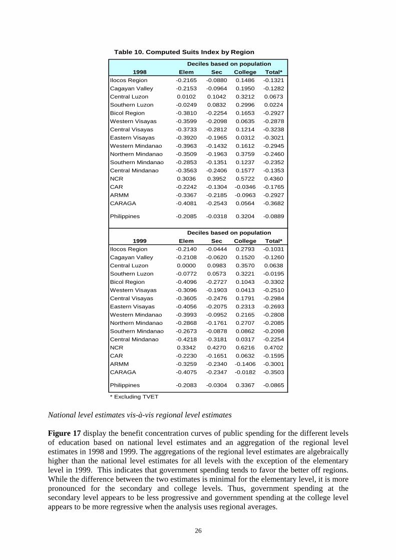
Note that the unit subsidy is influenced by two factors: demand for public education proxied by school enrolment and total public expenditures for a particular education level. Thus, it helps explain the inequality in the distribution of benefit incidence across regions. The progressivity of government spending at the elementary and secondary level is evidenced by the dominance of negative values of the Suits index for these levels across regions Table 10. To wit, government spending at the elementary level for both years is found to be progressive in all regions with the exception of NCR and Central Luzon in 1998 and 1999. Similarly, government spending at the secondary level is found to be progressive in all regions except NCR, Central Luzon and Southern Luzon in 1998 and 1999. In contrast, government spending on higher education is found to be regressive in all regions with the exception of CAR and ARMM in 1998 and ARMM and CARAGA in 1999. These findings indicate that college education in these few regions seems to cater more to the needs of the poorer households. This is indeed a surprising result considering that rarely do the poor reach higher education.

26

Table 10. Computed Suits Index by Region

Deciles based on population1998 Elem Sec College Total*

Ilocos Region -0.2165 -0.0880 0.1486 -0.1321Cagayan Valley -0.2153 -0.0964 0.1950 -0.1282Central Luzon 0.0102 0.1042 0.3212 0.0673Southern Luzon -0.0249 0.0832 0.2996 0.0224Bicol Region -0.3810 -0.2254 0.1653 -0.2927Western Visayas -0.3599 -0.2098 0.0635 -0.2878Central Visayas -0.3733 -0.2812 0.1214 -0.3238Eastern Visayas -0.3920 -0.1965 0.0312 -0.3021Western Mindanao -0.3963 -0.1432 0.1612 -0.2945Northern Mindanao -0.3509 -0.1963 0.3759 -0.2460Southern Mindanao -0.2853 -0.1351 0.1237 -0.2352Central Mindanao -0.3563 -0.2406 0.1577 -0.1353NCR 0.3036 0.3952 0.5722 0.4360CAR -0.2242 -0.1304 -0.0346 -0.1765ARMM -0.3367 -0.2185 -0.0963 -0.2927CARAGA -0.4081 -0.2543 0.0564 -0.3682

Philippines -0.2085 -0.0318 0.3204 -0.0889

Deciles based on population1999 Elem Sec College Total*

Ilocos Region -0.2140 -0.0444 0.2793 -0.1031Cagayan Valley -0.2108 -0.0620 0.1520 -0.1260Central Luzon 0.0000 0.0983 0.3570 0.0638Southern Luzon -0.0772 0.0573 0.3221 -0.0195Bicol Region -0.4096 -0.2727 0.1043 -0.3302Western Visayas -0.3096 -0.1903 0.0413 -0.2510Central Visayas -0.3605 -0.2476 0.1791 -0.2984Eastern Visayas -0.4056 -0.2075 0.2313 -0.2693Western Mindanao -0.3993 -0.0952 0.2165 -0.2808Northern Mindanao -0.2868 -0.1761 0.2707 -0.2085Southern Mindanao -0.2673 -0.0878 0.0862 -0.2098Central Mindanao -0.4218 -0.3181 0.0317 -0.2254NCR 0.3342 0.4270 0.6216 0.4702CAR -0.2230 -0.1651 0.0632 -0.1595ARMM -0.3259 -0.2340 -0.1406 -0.3001CARAGA -0.4075 -0.2347 -0.0182 -0.3503

Philippines -0.2083 -0.0304 0.3367 -0.0865

* Excluding TVET National level estimates vis-à-vis regional level estimates Figure 17 display the benefit concentration curves of public spending for the different levels of education based on national level estimates and an aggregation of the regional level estimates in 1998 and 1999. The aggregations of the regional level estimates are algebraically higher than the national level estimates for all levels with the exception of the elementary level in 1999. This indicates that government spending tends to favor the better off regions. While the difference between the two estimates is minimal for the elementary level, it is more pronounced for the secondary and college levels. Thus, government spending at the secondary level appears to be less progressive and government spending at the college level appears to be more regressive when the analysis uses regional averages.

27

Figure 17. Incidence of Public Spending on All Levels of Education, 1998 and 1999

Elementary Education

Secodary Education

Tertiary Education

Deciles on Population, 1998

0102030405060708090

100

1 2 3 4 5 6 7 8 9 10Cumulative % Distribution of Population

Cum

ulat

ive

% D

istr

ibut

ion

of S

ubsi

dy

PE line National Average W/ Regional Variation

Suits Index = -0.210



0102030405060708090

100


Cum

ulat

ive

% D

istr

ibut

ion

of S

ubsi

dy





0102030405060708090

100


Cum

ulat

ive

% D

istr

ibut

ion

of S

ubsi

dy





0

20

40

60

80

100


Cum

ulat

ive

% D

istr

ibut

ion

of S

ubsi

dy


Suits Index = -


0

20

40

60

80

100


Cum

ulat

ive

% D

istr

ibut

ion

of S

ubsi

dy


Suits Index =

Suits Index =


0102030405060708090

100


Cum

ulat

ive

% D

istr

ibut

ion

of

Subs

idy


Suits Index =

Suits Index =


28

6. Conclusion and Policy recommendations

Overall, government education spending is found to be progressive.

Using national averages, the distribution of education spending is progressive at the elementary and secondary level. On the contrary, it is regressive at the TVET and college levels.

The estimates based on the aggregation of regional level estimates are consistent with

these findings. However, the regional level estimates tend to suggest that government spending on education are less progressive (or more regressive) when the regional variation in government spending are factored into the analysis.

Surprisingly, government spending on higher education is found to be progressive in

ARMM, CAR, and CARAGA. This indicates that college education in these regions cater more to the needs of poorer households, thereby suggesting that the government should be more circumspect in cutting higher education subsidies in these areas.

While the progressivity of the total education is evident in all years, it declined, albeit

slowly, from 2001 onwards. This is associated with the decline in the share of elementary education in total education spending from 1999 onwards as the share of secondary education increased.

Education spending is well-targeted to the poor as evidenced by the share of

education budget that goes to basic education. It is really the poor that benefit more from government subsidies in basic education especially from elementary subsidies. Thus, the more government invest in elementary education, the greater gains poorer households get.

Increasing public resources to education while aligning intra-sectoral budget

allocations away from tertiary education towards primary education sounds good. Nevertheless, the results obtained from the regional benefit incidence analysis suggest that increasing college subsidy in regions where it is progressive can be justified.

The increase in budget allocations must be accompanied by increased enrolment by

poor households. Thus, issues that prevent the poor from accessing educational services must also be addressed.

Government intervention in the provision of basic education is undeniably a win-win

case for both the government and the society. Expanded investments in educational services both strengthen the national economy and improve the distribution of income and welfare by enabling the poor to have access to basic education. Further, it is very consistent with the commitment of the Philippine government to the Millennium Development Goal, i.e., to achieve universal primary education by 2015.

29

REFERENCES

Coady, D., M. Grosh and J. Hoddinott. 2004. Targeting of Transfers in Developing

Countries: Review of Lessons and Experience. Washington, D.C.: World Bank. Davoodi, H. E. Tiongson, and E. Asawanuchit. 2003. “How useful are benefit incidence

analysis of public education and health spending,” IMF Working Paper 03/227, International Monetary Fund, Washington D.C.

Demery, Lionel. 2000. Benefit Incidence: A Practitioner’s Guide. The World Bank.

Washington, D.C. Maglen, Leo and R. Manasan. 1999. Education Costs and Financing in the Philippines.

Philippine Education for the 21st Century. ADB/WB (Manila: ADB). Sabir, Muhammad. 2003. Benefit Incidence Analysis of Public Spending on Education. The

Journal, NIPA Karachi, Vol.8, No.3, p-49-67 van de Walle, Domique. 1996. Assessing the Welfare Impacts of Public Spending. Policy

Research Working Paper No. 1670. World Bank. Washington DC. van de Walle, Dominique. 1995. Public Spending and the Poor: What We Know, What We

Need to Know. Policy Research Working Paper No. 1476. World Bank. Washington DC. June.

30

ANNEX DATA REQUIREMENTS AND METHODOLOGY14

A. DATA REQUIREMENTS AND ISSUES INVOLVED

1. Government spending on a service (net of any cost recovery fees, out of pocket expenses by users of the service, or user fees)

BIA necessitates data on actual expenditures of the government on a certain service rather than budget allocation. The former represents the actual cost of services availed by the users and there is usually a big difference between the two. These data should be comprehensive as to include both recurrent and capital spending, and all levels of government (Davoodi et al, 2003). Spending data are ideally available in the relevant line agency or department. However, due to some reasons, these data cannot easily be obtained. Recent practice has been to use recurrent spending which frees analysts from the difficulty of estimating the flow of services/benefits from capital expenditures whose benefits extend beyond the usual period, i.e., one year. The problem comes in when capital budgets are large that they have significant impact on the benefit incidence of government expenditure. With regard to the levels of government spending, there are cases when spending is underreported because subnational data are not available. Further, government spending must be exclusive of cost recovery revenue before computing for unit subsidies. It should be noted, however, that, netting out of such revenue is on a case-to-case basis, i.e., depending on whether or not the revenue will be retained by the facility providing the service. If so, the revenue should be treated as additional amount to the value of the service (government subsidy) households get. But if it will be returned to the national coffer, the revenue should be netted out of the spending. The problem here is the difficulty in obtaining information on such fees and if ever available, it is not as reliable as the public expenditure data and is not in needed format, i.e., by income or consumption group. 2. Public utilization of the service

Users of a government service are referred to as beneficiaries of the service. For educational services, beneficiaries may include pupils enrolled in primary schools, and students enrolled in secondary and tertiary schools. In the case of health services, beneficiaries may be pregnant women visiting a commune health center, and infants and children immunized in a public clinic. Information on the number of beneficiaries can be obtained through a household survey or from the service providers per se but there can be discrepancies between the two. It may be wise to use the numbers from the latter as they are the ones reflected in the official reports. The choice of which to use will affect the findings of a benefit incidence analysis. For example, if official report gives higher enrolments than the household survey, a unit subsidy based on the former will be lower than the estimate derived using the latter. Thus, data must be used with caution. It would be good to compare the two datasets. If the numbers vary remarkably then the analysts should choose the more reliable source of information.

14 Draws heavily from Demery (2000) and Davoodi et al (2003)

31

3. Socio-economic characteristics of the population using the service

Information on the socioeconomic characteristics of the population using the service is useful when imputing or attributing a unit subsidy to beneficiaries because it gives idea on how government subsidies are distributed across individuals or households. Through it, analysis on the distributional impact of a subsidy is facilitated. Such information is not available from the service providers but household surveys such as Family Income and Expenditure Survey (FIES) and Annual Poverty Indicators Survey (APIS) have it. However, data users should be cautious in using information from these surveys as there may be biases in the data and even inconsistencies when compared with official reports.

Biases in data may arise due to sample design or structure of questionnaire that was used. One common example of these biases is found in data on the use of health services particularly curative health care. Since illness and injury are self-reported in most surveys, biases may result if poorer respondents do not report those illnesses, which they consider as ordinary, and richer respondents do otherwise. The poor would appear not to benefit from a certain health service but in reality, they fail to see the need for it. These biases, if not addressed, will distort the estimate for benefit incidence. Other data biases root from the sampling design used for the survey. Samples may not be able to capture rare events such as tertiary enrolments or in-patient health visits that estimates for service use is not accurate. Demery (2000) cited university enrolment as an example for this wherein serious underestimation occurs because the students are living outside the sampling frame.

Aside from these data biases, combining unit subsidy estimates based on official statistics and public utilization data obtained from household surveys becomes a concern when data are not consistently disaggregated, i.e., the disaggregation of one data set is different from that of another data set. Data users should be able to match these data sets so as to arrive at an accurate benefit incidence analysis. B. METHODOLOGY Step 1. Estimation of the unit subsidy of providing a certain service based on official reports on public spending on the service in question The average unit cost of providing a public service is obtained by dividing government net spending on the service by the total number of users of the service. Step 2. Imputation of the unit subsidy to households or individuals identified as beneficiaries of the service The unit subsidy derived in Step 1 is simply “attributed” or “imputed” to households or individuals identified as beneficiaries of the service. In this sense, each beneficiary gains an in-kind transfer equivalent to the unit subsidy. Step 3. Ranking of individuals or households according to a welfare indicator and aggregation of beneficiaries into sub-groups, oftentimes quintiles, of the population to see distributional impact of government spending/to compare how the subsidy is distributed across such groups

32

Individuals or households are arranged from poorest to richest based on a welfare indicator such as household income or expenditure expressed in per capita terms. They are then aggregated into sub-groups (e.g. quintiles or deciles) to get an idea whether public spending is well targeted to the poorest portion of the population. The grouping can be done either across individuals or across households. For example, aggregating individuals by decile (quintile) is done by dividing individuals into ten (five) sub-groups of equal size. The richest 10 percent of the population is found in the top decile while the poorest 10 percent is in the bottom decile. The same procedure can be applied when aggregating across households. The choice between aggregating by individuals or households depends on the service in question. It should be noted that when dealing with services that are provided to individuals (e.g. education and health services), grouping by individuals is appropriate to use. Otherwise, the results could be misleading. It might appear that a subsidy to a certain service is pro-poor because poorer households tend to have more members than richer households. On the one hand, grouping by households is recommended when dealing with services that are used at the household level (e.g. waterworks system or drinking water services). Nevertheless, the analyst still has the prerogative on what to use but it is worth mentioning that estimating benefit incidence using the two alternative methods of aggregation and comparing the findings gives more insights. Step 4. Derivation of the distribution of benefits by multiplying the average benefit calculated previously by the number of users of the service in each income or consumption group The assumption here is that the average benefit from or unit subsidy of a service is the same for all income or consumption levels. According to Davoodi (2003), this assumption implies two problems: i) the quantity of service may vary across users either because of variation in spending or the cost of producing the service; and ii) the value that users give on certain service may also vary across households. For illustrative purposes, the procedure on how to estimate benefit incidence is given below:

X ESE

EE

Sj iji

ii

ij

ii

i

≡ ≡= =∑ ∑

1

3

1

3

j = 1,…,10 (1)

where Xj is the value of the total education subsidy or benefit incidence accruing to income group j; Eij is the number of enrolled pupils/students in education level i from group j; Ei is the total number of enrolled students in a certain education level from all income groups; and Si is government net spending on education level i (with fees and other cost recovery netted out). The index i ranges from 1 to 4 (i = 1,..,4) denoting the levels of education such as primary, secondary, tertiary, and TVET.

The ratio Si/Ei gives the unit subsidy or cost per pupil/student of providing education at level i. The unit subsidy is the same across income groups but it varies across education levels. Expectedly, it also varies markedly by region because educational services in urban areas usually attract higher subsidies compared to those of rural areas. Moreover, services in the capital city often get better financing than in other urban areas (Demery, 2000). Such variations in unit subsidies result in inequalities in the distribution of benefits. Analysis that includes regional variations provides more insights but this is not always feasible given

33

limited data. If regional data are not available, Equation (1) becomes the only basis for analysis. Otherwise, Equation (2) can be used as well.

∑∑==

≡3

11 iik

i

ijkn

kj S

EE

X (2)

where k is the index that denotes the region. The share of the total education subsidy (S) accruing to the group is given by:

xEE

SS

e sjk

nijk

i

ik

i k

n

ijk iki

≡⎛

⎝⎜⎜

⎞

⎠⎟⎟ ≡

= = = =∑∑ ∑∑

1 1

3

1 1

3

The share summarizes the overall inequality in benefit incidence as determined by two factors: the share of the group in total enrollments at each level of education and in each region (eijk), and the share of each level of education and region in total education spending (sik). The e’s and s’s reflect the behavior of households in terms of enrolment decisions and government in terms of budget allocations across regions and levels of schooling, respectively.

34

APPENDIX

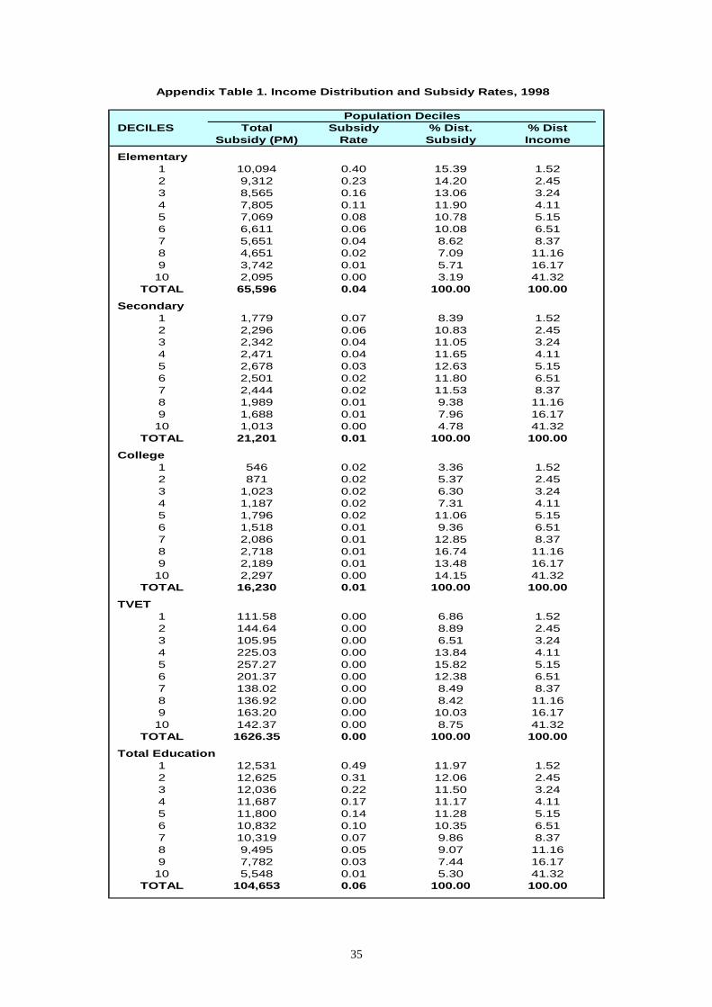
35

Appendix Table 1. Income Distribution and Subsidy Rates, 1998

Population DecilesDECILES Total Subsidy % Dist. % Dist

Subsidy (PM) Rate Subsidy Income

Elementary1 10,094 0.40 15.39 1.522 9,312 0.23 14.20 2.453 8,565 0.16 13.06 3.244 7,805 0.11 11.90 4.115 7,069 0.08 10.78 5.156 6,611 0.06 10.08 6.517 5,651 0.04 8.62 8.378 4,651 0.02 7.09 11.169 3,742 0.01 5.71 16.1710 2,095 0.00 3.19 41.32

TOTAL 65,596 0.04 100.00 100.00

Secondary1 1,779 0.07 8.39 1.522 2,296 0.06 10.83 2.453 2,342 0.04 11.05 3.244 2,471 0.04 11.65 4.115 2,678 0.03 12.63 5.156 2,501 0.02 11.80 6.517 2,444 0.02 11.53 8.378 1,989 0.01 9.38 11.169 1,688 0.01 7.96 16.1710 1,013 0.00 4.78 41.32

TOTAL 21,201 0.01 100.00 100.00

College1 546 0.02 3.36 1.522 871 0.02 5.37 2.453 1,023 0.02 6.30 3.244 1,187 0.02 7.31 4.115 1,796 0.02 11.06 5.156 1,518 0.01 9.36 6.517 2,086 0.01 12.85 8.378 2,718 0.01 16.74 11.169 2,189 0.01 13.48 16.1710 2,297 0.00 14.15 41.32

TOTAL 16,230 0.01 100.00 100.00

TVET1 111.58 0.00 6.86 1.522 144.64 0.00 8.89 2.453 105.95 0.00 6.51 3.244 225.03 0.00 13.84 4.115 257.27 0.00 15.82 5.156 201.37 0.00 12.38 6.517 138.02 0.00 8.49 8.378 136.92 0.00 8.42 11.169 163.20 0.00 10.03 16.1710 142.37 0.00 8.75 41.32

TOTAL 1626.35 0.00 100.00 100.00

Total Education1 12,531 0.49 11.97 1.522 12,625 0.31 12.06 2.453 12,036 0.22 11.50 3.244 11,687 0.17 11.17 4.115 11,800 0.14 11.28 5.156 10,832 0.10 10.35 6.517 10,319 0.07 9.86 8.378 9,495 0.05 9.07 11.169 7,782 0.03 7.44 16.1710 5,548 0.01 5.30 41.32

TOTAL 104,653 0.06 100.00 100.00

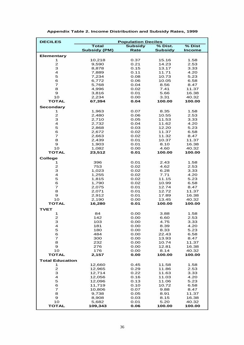
36

Appendix Table 2. Income Distribution and Subsidy Rates, 1999

DECILES Population DecilesTotal Subsidy % Dist. % Dist

Subsidy (PM) Rate Subsidy Income

Elementary1 10,218 0.37 15.16 1.582 9,590 0.21 14.23 2.533 8,878 0.15 13.17 3.334 7,889 0.11 11.71 4.205 7,234 0.08 10.73 5.236 6,772 0.06 10.05 6.587 5,768 0.04 8.56 8.478 4,996 0.02 7.41 11.379 3,816 0.01 5.66 16.38

10 2,234 0.00 3.31 40.32TOTAL 67,394 0.04 100.00 100.00

Secondary1 1,963 0.07 8.35 1.582 2,480 0.06 10.55 2.533 2,710 0.05 11.53 3.334 2,732 0.04 11.62 4.205 2,868 0.03 12.20 5.236 2,672 0.02 11.37 6.587 2,663 0.02 11.32 8.478 2,439 0.01 10.37 11.379 1,903 0.01 8.10 16.38

10 1,082 0.00 4.60 40.32TOTAL 23,512 0.01 100.00 100.00

College1 396 0.01 2.43 1.582 753 0.02 4.62 2.533 1,023 0.02 6.28 3.334 1,255 0.02 7.71 4.205 1,815 0.02 11.15 5.236 1,790 0.02 10.99 6.587 2,075 0.01 12.74 8.478 2,071 0.01 12.72 11.379 2,912 0.01 17.89 16.38

10 2,190 0.00 13.45 40.32TOTAL 16,280 0.01 100.00 100.00

TVET1 84 0.00 3.88 1.582 142 0.00 6.60 2.533 103 0.00 4.75 3.334 181 0.00 8.39 4.205 180 0.00 8.33 5.236 484 0.00 22.43 6.587 300 0.00 13.93 8.478 232 0.00 10.74 11.379 276 0.00 12.81 16.38

10 176 0.00 8.14 40.32TOTAL 2,157 0.00 100.00 100.00

Total Education1 12,660 0.45 11.58 1.582 12,965 0.29 11.86 2.533 12,714 0.22 11.63 3.334 12,056 0.16 11.03 4.205 12,096 0.13 11.06 5.236 11,719 0.10 10.72 6.587 10,806 0.07 9.88 8.478 9,738 0.05 8.91 11.379 8,908 0.03 8.15 16.38

10 5,682 0.01 5.20 40.32TOTAL 109,343 0.06 100.00 100.00

Benefit Incidence of Public Spending on Education in … · DISCUSSION PAPER SERIES NO. 2007-09...

Documents

Transcript of Benefit Incidence of Public Spending on Education in … · DISCUSSION PAPER SERIES NO. 2007-09...