Benefit Cost Analysis

DRAFT, 3rd May 2017

Benefit Cost Analysis

Boosting Biosecurity Defences

of 49

Author contact details

Name: Dr David C. Cook

Address: PO Box 1231, Bunbury WA 6231

Phone: (08) 9780 6179

Fax: (08) 9780 6100

Email: [email protected]

DAFWA contact details

Department of Agriculture and Food

Locked Bag 4

Bentley Delivery Centre WA 6983

Phone: +61 (0)8 9368 3333

Fax: +61 (0)8 9474 2405

Email: [email protected]

Web: www.agric.wa.gov.au

Disclaimer

The Chief Executive Officer of the Department of Agriculture and Food and the

State of Western Australia accept no liability whatsoever by reason of negligence

or otherwise arising from the use or release of this information or any part of it.

Copyright © Western Australian Agriculture Authority, 2017

mailto:[email protected]

http://www.agric.wa.gov.au/

of 49

Table of contents

1. Executive Summary ........................................................................................ 6

2. Introduction ..................................................................................................... 8

3. Scope .............................................................................................................. 9

4. Methods ........................................................................................................ 10

4.1. Derivation of benefits .......................................................................................... 10

4.2 Project costs ........................................................................................................ 14

4.3. Attribution ........................................................................................................... 15

5. Results .......................................................................................................... 16

5.1. Subproject 1: State Biosecurity Strategy ............................................................. 16

5.2. Subproject 2: E-Surveillance for pests and diseases in the WA grains industry .. 17

5.3. Subproject 3: E-Surveillance for pests and diseases of the WA grape industry... 20

5.4. Subproject 4: Early detection of emergency animal diseases ............................. 22

5.5. Subproject 5: Agricultural weed surveillance in the South West to protect industry

profitability ................................................................................................................. 25

5.6. Subproject 6: Build capacity to respond and recover from emergency pest and

disease incidents ....................................................................................................... 27

5.7. Subproject 7: Awareness and compliance with new biosecurity legislation ......... 28

5.8. Subproject 8: Biosecurity research and development fund ................................. 29

5.9. Subproject 9: Transforming regional biosecurity response .................................. 32

5.10. Subproject 10: Eradication of Medfly in Carnarvon ........................................... 33

5.11. Subproject 11: Wild dog control measures ........................................................ 35

5.12. Synthesis .......................................................................................................... 36

6. Conclusion .................................................................................................... 40

7. References.................................................................................................... 41

8. Appendix ....................................................................................................... 44

of 49

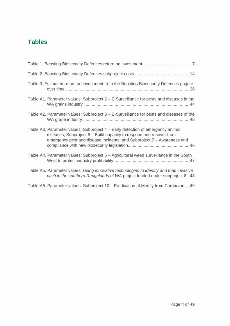
Tables

Table 1. Boosting Biosecurity Defences return on investment ......................................... 7

Table 2. Boosting Biosecurity Defences subproject costs ............................................. 14

Table 3. Estimated return on investment from the Boosting Biosecurity Defences project

over time ....................................................................................................... 38

Table A1. Parameter values: Subproject 2 – E-Surveillance for pests and diseases in the

WA grains industry ........................................................................................ 44

Table A2. Parameter values: Subproject 3 – E-Surveillance for pests and diseases of the

WA grape industry ......................................................................................... 45

Table A3. Parameter values: Subproject 4 – Early detection of emergency animal

diseases; Subproject 6 – Build capacity to respond and recover from

emergency pest and disease incidents; and Subproject 7 – Awareness and

compliance with new biosecurity legislation................................................... 46

Table A4. Parameter values: Subproject 5 – Agricultural weed surveillance in the South

West to protect industry profitability ............................................................... 47

Table A5. Parameter values: Using innovative technologies to identify and map invasive

cacti in the southern Rangelands of WA project funded under subproject 8 .. 48

Table A6. Parameter values: Subproject 10 – Eradication of Medfly from Carnarvon .... 49

of 49

Figures

Figure 1. Cumulative diffusion of innovations model (Rogers, 2010) ............................. 15

Figure 2. Estimated benefit of subproject 2 ................................................................... 18

Figure 3. Estimated return per dollar invested in subproject 2 ....................................... 19



Figure 6. Estimated benefit of subprojects 4, 6 and 7 .................................................... 23

Figure 7. Estimated return per dollar invested in subprojects 4, 6 and 7 ....................... 24



Figure 10. Estimated benefit of Using innovative technologies to identify and map

invasive cacti in the southern Rangelands of WA project funded under

subproject 8 .................................................................................................. 30

Figure 11. Estimated return per dollar invested in the Using innovative technologies to

identify and map invasive cacti in the southern Rangelands of WA project

funded under subproject 8 ............................................................................. 31

Figure 12. Estimated benefit of subproject 10 ............................................................... 33

Figure 13. Estimated return per dollar invested in subproject 10 ................................... 34

Figure 14. Distribution of simulated pest and disease impacts with and without the BBD

project ........................................................................................................... 36

Figure 15. Estimated return on investment from the BBD project .................................. 37

Figure 16. Sensitivity analysis ...................................................................................... 39

of 49

1. Executive Summary

− This analysis estimates the likely producer benefits created as a result of the

$26.9 million Boosting Biosecurity Defences project. The 11 subprojects

involved in the project receive a combined $20 million in funding from the

Government of Western Australia’s Seizing the Opportunity Royalties for

Regions initiative.

− A bioeconomic model is used to estimate the likely pest and disease damage

avoided through eight of the 11 subproject activities. The avoided damages

are compared to costs to provide a benefit cost analysis. Results are

summarised in Table 1.

− The highest net benefit is created by subprojects 4, 6 and 7 (Early detection

of emergency animal diseases, Build capacity to respond and recover from

emergency pest and disease incidents, and Awareness and compliance with

new biosecurity legislation, respectively), with a combined net benefit of

$106.3 million over 30 years.

− The highest return per dollar invested is created by subproject 3

(E-Surveillance for pests and diseases of the WA grape industry). This

relatively small subproject is expected to produce $56.40 for every dollar

invested in it.

− Combining analyses of the subprojects, an aggregate benefit cost

assessment of the Boosting Biosecurity Defences project estimates the

project will generate a net benefit in excess of $240 million over the next 30

years.

− Approximately $17.40 of producer benefits are created for ever $1.00

invested in the Boosting Biosecurity Defences project.

of 49

Table 1. Boosting Biosecurity Defences return on investment

Subproject

Present value

of costs

($ million)

Present value

of benefits

($ million)

Net present

value

($ million)

Benefit cost

ratio

1. State Biosecurity

Strategy na na na na

2. E-Surveillance for pests

and diseases in the WA

grains industry

1.73 36.50 34.77 22.77

3. E-Surveillance for pests

and diseases of the WA

grape industry

1.08 61.09 60.01 56.40

4. Early detection of

emergency animal

diseases

6. Build capacity to respond

and recover from

emergency pest and

disease incidents

7. Awareness and

compliance with new

biosecurity legislation

7.36 113.63 106.27 15.44

5. Agricultural weed

surveillance in the South

West to protect industry

profitability

0.95 34.11 33.16 38.03

8. Biosecurity research and

development fund -

Using innovative

technologies to identify

and map invasive cacti

in the southern

Rangelands of WA

0.15 0.37 0.22 2.44

9. Transforming regional

biosecurity response na na na na

10. Eradication of Medfly in

Carnarvon 3.48 10.95 7.47 3.38

11. Wild dog control

measures na na na na

Boosting Biosecurity

Defences 14.76 256.64 241.89 17.39

of 49

2. Introduction

This report estimates the likely return on investment in the Boosting Biosecurity

Defences project, henceforth BBD, funded under the Government of Western

Australia’s Seizing the Opportunity Royalties for Regions (RfR) initiative. This

project involves 11 separate activities developed by the Department of

Agriculture and Food WA (DAFWA), the WA Biosecurity Council and key industry

and community stakeholders.

The total investment received for the BBD project is $26.9 million to be spent

between 2013/14 and 2016/17. This includes $6.9 million of cash and in-kind

contributions from the Carnarvon Grower Association, Horticulture Innovation

Australia Ltd., State Natural Resource Management Office, Council of Grain

Grower Organisations and DAFWA. The investment from RfR is $20.0 million.

The economic and social benefits to the State produced by the BBD project will

accrue over time from early detection and rapid response to pest and disease

incursions. This will avoid producer cost increases and yield reductions over

time, reduce the likelihood of losing area-freedom status and reduce the time it

takes to regain market access if it is lost.

An economic impact simulation model is used to estimate the likely returns to

WA agricultural industries from BBD subprojects achieving their intended

outcomes. Results are aggregated to produce a benefit cost analysis for the

BBD project as a whole.

Results indicate that a net benefit of $241.9 million will be created by the BBD

project over a period of 30 years. The highest net benefit is created by

subprojects 4, 6 and 7 (Early detection of emergency animal diseases, Build

capacity to respond and recover from emergency pest and disease incidents,

and Awareness and compliance with new biosecurity legislation, respectively).

However, the highest return per dollar invested is created by subproject 3 (E-

Surveillance for pests and diseases of the WA grape industry).

The simulation model used to predict the change in invasive species impacts

over time attributable to the BBD project is sensitive to changes in several key

parameters. These include the probabilities of invasive species entry and

establishment, likelihood of detection and several spread parameters. These

sensitivities and a lack of certain parameter information mean results are

uncertain.

of 49

3. Scope

The purpose of this assessment is to estimate the likely agricultural benefits

produced by the BBD project over a 30-year period if each subproject attains its

intended goals. The technical challenges faced in reaching these goals are not

considered as part of the scope for this document; rather what are the likely

gains in them doing so.

Subproject goals relate to restricting the abundance, distribution and impact of

plant and animal species of biosecurity significance to levels below what they

otherwise would have been without the RfR initiative. These include species that

have already become established in the State, and those that remain exotic to it.

Numerous terms have been used to describe species of biosecurity importance,

including “non-indigenous”, “non-native”, “alien”, “exotic”, “invasive”, “noxious”,

“nuisance”, and “weed”. This has caused confusion and misuse of existing

terminology, with the term ‘invasive’ being particularly problematic as ecologists

use it in reference to species that rapidly spread beyond the location of initial

establishment. In contrast, policy and legal documents tend to refer to invasive

species as those causing negative effects to human beings, even though

invasiveness of a species does not necessarily predict its impact (Ricciardi and

Cohen, 2007).

For the purpose of this analysis, an invasive species is defined as a species that

does not naturally occur in a specific area and whose introduction does or is

likely to cause net negative social welfare consequences. Social welfare, itself

difficult to define, would ideally encompasses environmental, economic and

social impacts (both intended and unintended) of BBD activities. However, due

to time constraints, this assessment is limited to agricultural benefits.

of 49

4. Methods

4.1. Derivation of benefits

This section contains details of the methodology used to assess the return on

investment in the BBD project. In particular, the simulation model used to predict

the change in invasive species impacts over time attributable to the project is

detailed. It is intended that this will invite critical comment in an appropriate

context to refine and potentially build on the assessment.

Readers chiefly concerned with the assessment results may wish to proceed to

Section 5 where estimated benefits of specific BBD subprojects are revealed.

Predicting invasive species impacts before they occur involves a great deal of

uncertainty. Indeed, even after they occur, when we have actual impact data, we

are not necessarily able to make better predictions. A data set only tells us

about one possible set of outcomes from a wide range of possibilities. It follows

that forecasting likely reductions in invasive species impacts resulting from a

broad suite of investments, as with the BBD project, is even more challenging.

Rather than developing a simulation model from scratch to estimate reductions in

invasive species impacts over time, an existing model is used that has formed

the basis of many peer-reviewed economic assessments (e.g. Cook et al.,

2013a, Cook and Fraser, 2014, Cook et al., 2013b, Cook et al., 2011a, Cook,

2008, Cook et al., 2011b). The model has the capability of calculating the

economic impacts of a wide variety of pests and diseases over time with and

without different prevention and control activities.

Within the model, agricultural areas are denoted i. In the case of exotic species,

pest and disease arrival events in these regions are generated using entry and

establishment probabilities denoted 𝑧𝑒𝑛𝑡 and 𝑧𝑒𝑠𝑡, respectively. A Markov chain

process is used to change 𝑧𝑒𝑛𝑡 and 𝑧𝑒𝑠𝑡 over time according to a vector of

transitional probabilities that describe the likelihood of moving from one pest

state to another. The probabilities 𝑧𝑒𝑛𝑡 and 𝑧𝑒𝑠𝑡 are combined to form a

probability of arrival for a specific region i, 𝑧𝑖:

𝑧𝑖 = 𝑧𝑒𝑛𝑡 × 𝑧𝑒𝑠𝑡 where 0 < 𝑧𝑖 < 1. (1)

of 49

A stratified diffusion process combining both short and long distance dispersal is

used to predict the area potentially affected by pests and diseases post-

establishment in each region i in time period t, 𝐴𝑖𝑡1.

This method of calculating the area occupied by an organism over time has been

shown to provide a reasonable approximation of spread for a wide range of

species (Okubo and Levin, 2002, Dwyer, 1992, Holmes, 1993, McCann et al.,

2000, Cook et al., 2011a). It assumes that an invasion diffusing from a point

source will eventually reach a constant asymptotic radial spread rate of 2√𝑟𝑖𝐷𝑖𝑗

in all directions, where 𝑟𝑖 describes a growth factor for an invasive species per

year in region i (assumed constant over all affected sites) and 𝐷𝑖𝑗 is a diffusion

coefficient for an affected site j in region i (assumed constant over time) (Lewis,

1997, Shigesada and Kawasaki, 1997, Cook et al., 2011a, Hengeveld, 1989).

Hence, assume that the site of the original outbreak (i.e. the first of a probable

series of sites, j) takes place in a homogenous environment in region i and

expands by a diffusive process such that area affected at time t, 𝑎𝑖𝑗𝑡, can be

predicted by:

𝑎𝑖𝑗𝑡 = 𝑧𝑖 [𝜋(2𝑡√𝑟𝑖𝐷𝑖𝑗)2

] = 𝑧𝑖(4𝐷𝑖𝑗𝜋𝑟𝑖𝑡2). (2)

For practical purposes, an estimate of 𝐷𝑖𝑗 can be derived from the mean

dispersal distance (𝛿�̅�𝑗)at an incursion site, where 𝐷𝑖𝑗 =2(�̅�𝑖𝑗)2

𝜋𝑡 (Andow et al.,

1990, Cook et al., 2011b, Cook et al., 2010). The variable 𝛿�̅�𝑗 is the site-specific

average distance (in metres) over which dispersal events occur.

The density of an outbreak within 𝑎𝑖𝑗𝑡 influences the control measures required to

counter its effects, and thus partially determines the value of 𝐴𝑖𝑡. Assume that in

each site j in region i affected, the density, 𝑁𝑖𝑗𝑡, grows over time period t

following a logistic growth curve until the carrying capacity of the host

environment, 𝐾𝑖𝑗, is reached:

𝑁𝑖𝑗𝑡 =𝐾𝑖𝑗𝑁𝑖𝑗

𝑚𝑖𝑛𝑒𝑟𝑖𝑡

𝐾𝑖𝑗+𝑁𝑖𝑗𝑚𝑖𝑛(𝑒𝑟𝑖𝑡−1)

. (3)

1 Parameter estimates for specific species appear in following sections. Due to the uncertainty

surrounding some of these parameters, they are specified using a range of distributional forms,

rather than simple point estimates. Types of distributions used in this report include: (a) pert – a

type of beta distribution specified using minimum, most likely (or skewness) and maximum

values; (b) uniform – a rectangular distribution bounded by minimum and maximum values; (c)

binomial – returning a zero (failure) or one (success) based on a number of trials and the

probability of a success; (d) discrete - a distribution in which several discrete outcomes and their

probabilities of occurrence are specified; (e) Poisson - a discrete distribution returning only

integer values greater than or equal to zero with a specified mean value.

of 49

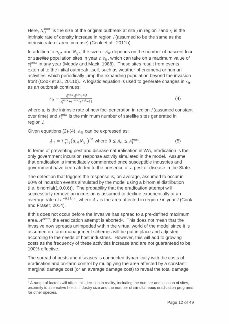
Here, 𝑁𝑖𝑗𝑚𝑖𝑛 is the size of the original outbreak at site j in region i and 𝑟𝑖 is the

intrinsic rate of density increase in region i (assumed to be the same as the

intrinsic rate of area increase) (Cook et al., 2011b).

In addition to 𝑎𝑖𝑗𝑡 and 𝑁𝑖𝑗𝑡, the size of 𝐴𝑖𝑡 depends on the number of nascent foci

or satellite population sites in year t, 𝑠𝑖𝑡, which can take on a maximum value of

𝑠𝑖𝑚𝑎𝑥 in any year (Moody and Mack, 1988). These sites result from events

external to the initial outbreak itself, such as weather phenomena or human

activities, which periodically jump the expanding population beyond the invasion

front (Cook et al., 2011b). A logistic equation is used to generate changes in 𝑠𝑖𝑡

as an outbreak continues:

𝑠𝑖𝑡 =𝑠𝑖

𝑚𝑎𝑥𝑠𝑖𝑚𝑖𝑛𝑒𝜇𝑖𝑡

𝑠𝑖𝑚𝑎𝑥+𝑠𝑖

𝑚𝑖𝑛(𝑒𝜇𝑖𝑡−1) (4)

where 𝜇𝑖 is the intrinsic rate of new foci generation in region i (assumed constant

over time) and 𝑠𝑖𝑚𝑖𝑛 is the minimum number of satellite sites generated in

region i.

Given equations (2)-(4), 𝐴𝑖𝑡 can be expressed as:

𝐴𝑖𝑡 = ∑ (𝑎𝑖𝑗𝑡𝑁𝑖𝑗𝑡)𝑠𝑖𝑡𝑚

𝑗=1 where 0 ≤ 𝐴𝑖𝑡 ≤ 𝐴𝑖𝑚𝑎𝑥. (5)

In terms of preventing pest and disease naturalisation in WA, eradication is the

only government incursion response activity simulated in the model. Assume

that eradication is immediately commenced once susceptible industries and

government have been alerted to the presence of a pest or disease in the State.

The detection that triggers the response is, on average, assumed to occur in

60% of incursion events simulated by the model using a binomial distribution

(i.e. binomial(1.0,0.6)). The probability that the eradication attempt will

successfully remove an incursion is assumed to decline exponentially at an

average rate of 𝑒−0.15𝐴𝑖𝑡, where 𝐴𝑖𝑡 is the area affected in region i in year t (Cook

and Fraser, 2014).

If this does not occur before the invasive has spread to a pre-defined maximum

area, 𝐴𝑒𝑟𝑎𝑑, the eradication attempt is aborted2. This does not mean that the

invasive now spreads unimpeded within the virtual world of the model since it is

assumed on-farm management schemes will be put in place and adjusted

according to the needs of host industries. However, this will add to growing

costs as the frequency of these activities increase and are not guaranteed to be

100% effective.

The spread of pests and diseases is connected dynamically with the costs of

eradication and on-farm control by multiplying the area affected by a constant

marginal damage cost (or an average damage cost) to reveal the total damage

2 A range of factors will affect this decision in reality, including the number and location of sites,

proximity to alternative hosts, industry size and the number of simultaneous eradication programs

for other species.

of 49

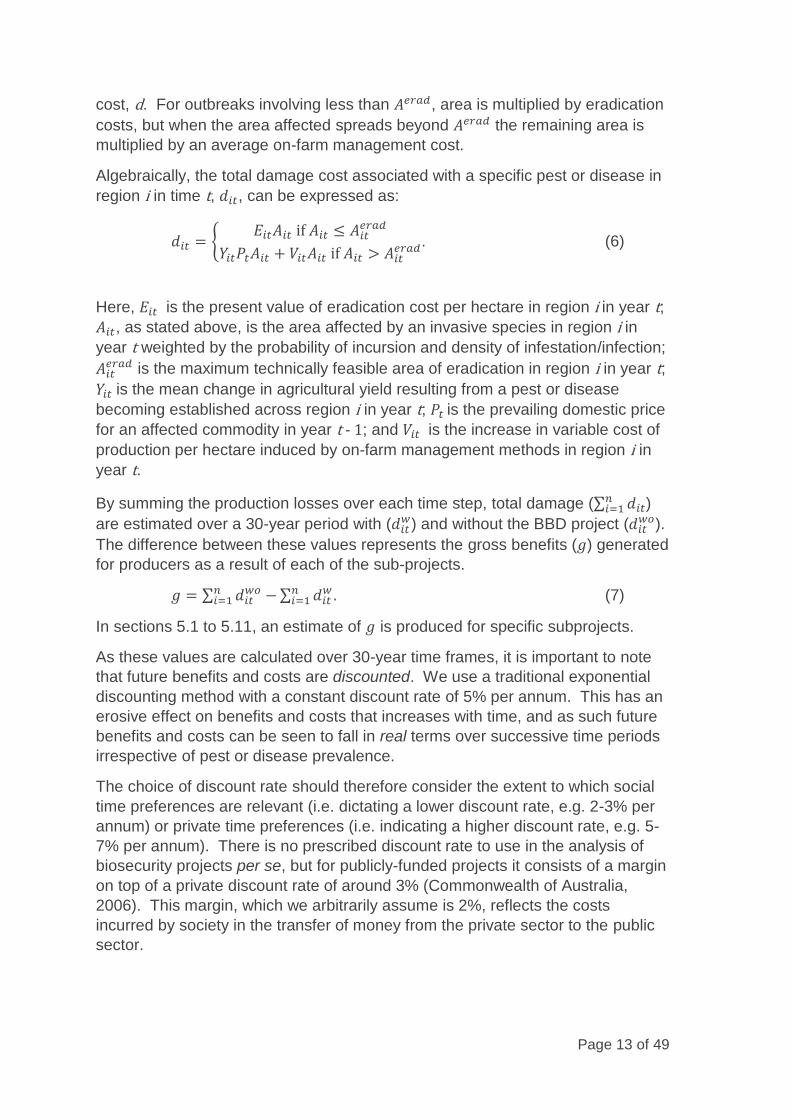
cost, d. For outbreaks involving less than 𝐴𝑒𝑟𝑎𝑑, area is multiplied by eradication

costs, but when the area affected spreads beyond 𝐴𝑒𝑟𝑎𝑑 the remaining area is

multiplied by an average on-farm management cost.

Algebraically, the total damage cost associated with a specific pest or disease in

region i in time t, 𝑑𝑖𝑡, can be expressed as:

𝑑𝑖𝑡 = {𝐸𝑖𝑡𝐴𝑖𝑡 if 𝐴𝑖𝑡 ≤ 𝐴𝑖𝑡

𝑒𝑟𝑎𝑑

𝑌𝑖𝑡𝑃𝑡𝐴𝑖𝑡 + 𝑉𝑖𝑡𝐴𝑖𝑡 if 𝐴𝑖𝑡 > 𝐴𝑖𝑡𝑒𝑟𝑎𝑑. (6)

Here, 𝐸𝑖𝑡 is the present value of eradication cost per hectare in region i in year t; 𝐴𝑖𝑡, as stated above, is the area affected by an invasive species in region i in

year t weighted by the probability of incursion and density of infestation/infection;

𝐴𝑖𝑡𝑒𝑟𝑎𝑑 is the maximum technically feasible area of eradication in region i in year t;

𝑌𝑖𝑡 is the mean change in agricultural yield resulting from a pest or disease

becoming established across region i in year t; 𝑃𝑡 is the prevailing domestic price

for an affected commodity in year t - 1; and 𝑉𝑖𝑡 is the increase in variable cost of

production per hectare induced by on-farm management methods in region i in

year t.

By summing the production losses over each time step, total damage (∑ 𝑑𝑖𝑡𝑛𝑖=1 )

are estimated over a 30-year period with (𝑑𝑖𝑡𝑤) and without the BBD project (𝑑𝑖𝑡

𝑤𝑜).

The difference between these values represents the gross benefits (𝑔) generated

for producers as a result of each of the sub-projects.

𝑔 = ∑ 𝑑𝑖𝑡𝑤𝑜 −𝑛

𝑖=1 ∑ 𝑑𝑖𝑡𝑤𝑛

𝑖=1 . (7)

In sections 5.1 to 5.11, an estimate of 𝑔 is produced for specific subprojects.

As these values are calculated over 30-year time frames, it is important to note

that future benefits and costs are discounted. We use a traditional exponential

discounting method with a constant discount rate of 5% per annum. This has an

erosive effect on benefits and costs that increases with time, and as such future

benefits and costs can be seen to fall in real terms over successive time periods

irrespective of pest or disease prevalence.

The choice of discount rate should therefore consider the extent to which social

time preferences are relevant (i.e. dictating a lower discount rate, e.g. 2-3% per

annum) or private time preferences (i.e. indicating a higher discount rate, e.g. 5-

7% per annum). There is no prescribed discount rate to use in the analysis of

biosecurity projects per se, but for publicly-funded projects it consists of a margin

on top of a private discount rate of around 3% (Commonwealth of Australia,

2006). This margin, which we arbitrarily assume is 2%, reflects the costs

incurred by society in the transfer of money from the private sector to the public

sector.

of 49

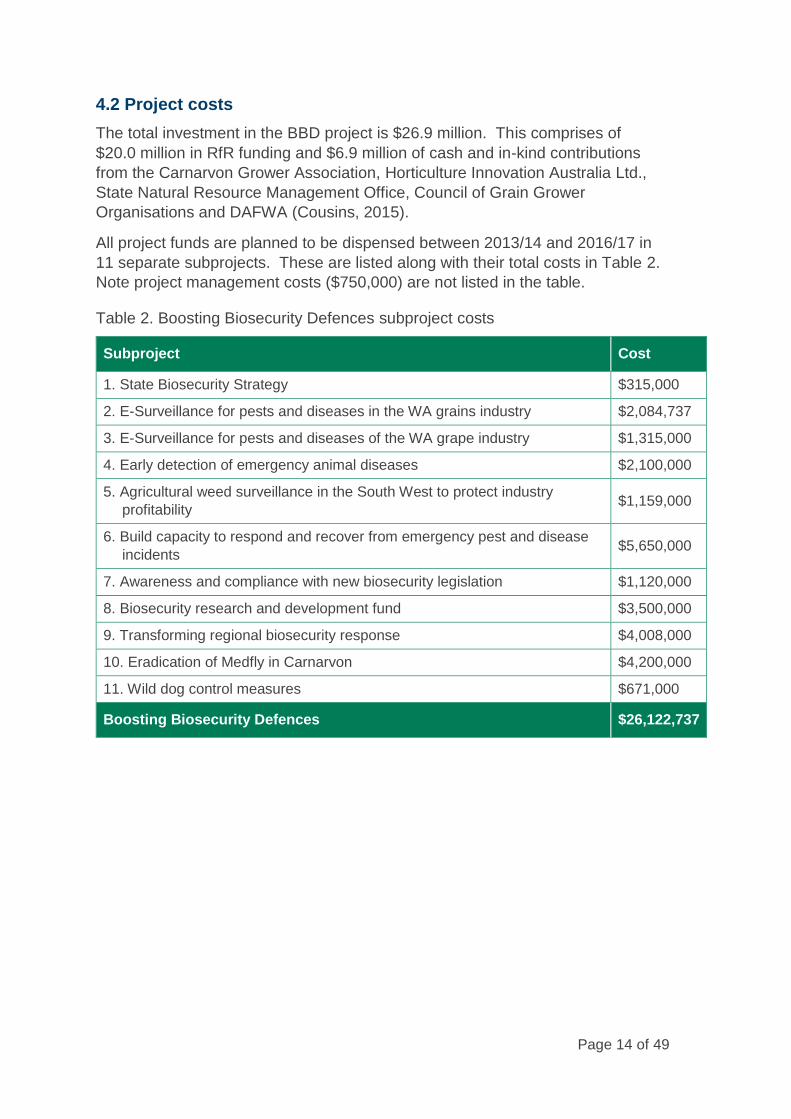
4.2 Project costs

The total investment in the BBD project is $26.9 million. This comprises of

$20.0 million in RfR funding and $6.9 million of cash and in-kind contributions

from the Carnarvon Grower Association, Horticulture Innovation Australia Ltd.,

State Natural Resource Management Office, Council of Grain Grower

Organisations and DAFWA (Cousins, 2015).

All project funds are planned to be dispensed between 2013/14 and 2016/17 in

11 separate subprojects. These are listed along with their total costs in Table 2.

Note project management costs ($750,000) are not listed in the table.

Table 2. Boosting Biosecurity Defences subproject costs

Subproject Cost

1. State Biosecurity Strategy $315,000

2. E-Surveillance for pests and diseases in the WA grains industry $2,084,737

3. E-Surveillance for pests and diseases of the WA grape industry $1,315,000

4. Early detection of emergency animal diseases $2,100,000

5. Agricultural weed surveillance in the South West to protect industry

profitability $1,159,000

6. Build capacity to respond and recover from emergency pest and disease

incidents $5,650,000

7. Awareness and compliance with new biosecurity legislation $1,120,000

8. Biosecurity research and development fund $3,500,000

9. Transforming regional biosecurity response $4,008,000

10. Eradication of Medfly in Carnarvon $4,200,000

11. Wild dog control measures $671,000

Boosting Biosecurity Defences $26,122,737

of 49

0%

20%

40%

60%

80%

100%

0 5 10 15 20 25 30

Ad

op

tio

n

Time (yr)

Attribution

4.3. Attribution

The attribution rate apportions benefits specifically to the project, and is

dependent on the innovations of subprojects being adopted by producers and the

broader biosecurity community. This in turn depends on a host of factors,

including the availability of information about the innovation, adopter

characteristics (e.g. age, income, experience), characteristics of the social

system (e.g. management support, social attitudes to new ideas and technology),

and the networks through which innovations are communicated (Lyytinen and

Damsgaard, 2001).

Given the breadth of subprojects and diversity of activities being undertaken, to

truly map the adoption of methods and ideas produced by the BBD project would

require a detailed study of stakeholders and governments, their histories and

networking using multiple perspectives including political models, institutional

models and theories of team behaviour (Lyytinen and Damsgaard, 2001).

However, time and information constraints have prevented the derivation and

use of specific attribution curves for each subproject.

Rather, the approach taken was to use a generic attribution curve. The Rogers

diffusion of innovations curve, shown in cumulative form in Figure 1 (Rogers,

2010), is a standardised adoption curve used to describe the way new ideas,

products and production techniques are adopted within communities over time.

Diffusion of innovations theory has been used in the areas of public health,

communication, marketing, political science, and most other behavioural and

social science disciplines (Rogers et al., 2005). We use it here to summarise the

adoption of innovations from each of the BBD subprojects.

Figure 1. Cumulative diffusion of innovations model (Rogers, 2010)

of 49

5. Results

5.1. Subproject 1: State Biosecurity Strategy

5.2.1. Background

This subproject concerns the development of a WA Biosecurity Strategy for the

period 2015-25. The strategy, released on the 21st November 2016, provides a

broad framework to manage emerging and ongoing animal and plant pest and

disease risks, including weeds and zoonotic diseases. DAFWA developed the

strategy in partnership with the Department of Parks and Wildlife, Department of

Fisheries, Forest Products Commission and Department of Premier and Cabinet.

5.2.2. Cost

This subproject involves a total investment of $315 000. This consists of

$165 000 of DAFWA in-kind resources and $150 000 RfR funds.

5.2.3. Benefit

Not applicable.

5.2.4. Return on investment

Due to its general, non-specific nature, subproject 1 is not evaluated as part of

this assessment.

Note however that from an economics standpoint, the effectiveness of the

strategy is compromised by the use of the Invasion Impact Curve (Agriculture

Victoria, 2015) to guide investment decisions3.

3 The generalised invasion curve is an abstract sigmoid curve implying certainty between the

area affected by an invasive species and the time since its arrival in a new region.

Unsubstantiated and unexplained benefit cost ratios are put forward in Agriculture Victoria (2015)

that suggest returns to investment decline with the area occupied and that an appropriate

intervention (particularly by governments) lies in prevention and eradication. This is misleading

and has the potential to generate perverse outcomes when used as a policy guide.

https://www.agric.wa.gov.au/sites/gateway/files/WA%20Biosecurity%20Strategy%20%28A1756933%29.pdf

http://agriculture.vic.gov.au/__data/assets/image/0005/179051/invasion_curve_big.jpg

of 49

5.2. Subproject 2: E-Surveillance for pests and diseases in the WA

grains industry

5.2.1. Background

This subproject aims to enhance pest and disease surveillance and diagnostic

capacity for the WA grains industry. It will draw from existing databases

containing grains surveillance data and build a single database that can be

augmented through the use of citizen-science activities.

Specifically, this involves the development of a freely available smartphone App

called MyPest Guide that provides users with a real-time diagnostic tool. The

App encourages community involvement and greatly improves the effectiveness

of surveillance information provided by the general public. Using Bayesian

statistical methods to calculate the probability of area freedom from exotic pests

and diseases, the information gathered can reduce the probability of losing

market access.

In addition, subproject 2 aims to improve grains industry capacity to manage

exotic pest and disease incursions by identifying key threats and conducting a

gap analysis of people, infrastructure and resources, and planning remedial

actions.

5.2.2. Cost

This subproject involves a total investment of $2 084 000. This is made up of

$1 054 000 from DAFWA, $30 000 from the Council of Grain Grower

Organisations Western Australia (COGGO) and $1 000 000 from the RfR

initiative.

https://agspsrap31.agric.wa.gov.au/mypestguide/#/

of 49

5.2.3. Benefit

Figure 2. Estimated benefit of subproject 2


Using the mean of the distribution of model outputs shown in Figure 2 as our

measure of the gross value returned by the project (or 𝑔, from equation (7)), the

benefit cost ratio for subproject 2 is estimated to be between 1.2 and 22.8. The

assumptions on which this is based are detailed in Appendix 1, Table A1. The

distributions of benefit cost ratios produced by the subproject 2 are shown in

Figure 3 for 10, 20 and 30-year time frames. This assessment is based on a

small sample of the pests and diseases that could potentially be affected by the

subproject, but it is clear that the longer the time frame we consider the higher

the return on investment.

of 49

Figure 3. Estimated return per dollar invested in subproject 2

of 49

5.3. Subproject 3: E-Surveillance for pests and diseases of the WA

grape industry

5.3.1. Background

This subproject aims to influence the behaviour of wine and table grape

producers in relation to their understanding and participation in pest and disease

surveillance and diagnostic activities. It will promote the early detection of exotic

pests and disease incursions via a hybrid system for surveillance and diagnosis

activities combining elements of the DAFWA HortGuard™ and South Australian

Phylloxera systems.

This will involve the development and application of e-tools linking the MyPest

Guide smartphone app to viticulture. Over time, this will decrease the amount of

time new pest and disease arrivals are present before detection occurs and a

response is initiated. The damages prevented accrue over subsequent time

periods, and can be evaluated using a set of case study examples of some of the

species affected by the subproject.

5.3.2. Cost

This subproject involves a total investment of $1 315 000; comprising of

$479 000 from DAFWA and $836 000 from the RfR initiative.

5.3.3. Benefit


https://www.agric.wa.gov.au/plant-biosecurity/mypestguide-grapes-brochure

https://www.agric.wa.gov.au/plant-biosecurity/mypestguide-grapes-brochure

of 49


If we take the mean of the distribution of model outputs shown in Figure 4 as our

estimate of the gross value of the project, the benefit cost ratio for subproject 3 is

estimated to be 3.1 over 10 years, and as high as 56.4 over 30 years. The

assumptions on which this is based are detailed in Appendix 1, Table A2.

Distributions of benefit cost ratios produced by subproject 3 are shown in

Figure 5 for 10, 20 and 30-year time frames.


Despite this assessment being based on a small sample of the pests and

diseases that could potentially be affected by the subproject, it indicates a high

return on investment. Since WA is an importer of grapes a pathway exists

through which exotic pests and diseases can enter the State. It follows that the

pests and diseases potentially impacted by the subproject have a relatively high

probability of entry and establishment.

of 49

5.4. Subproject 4: Early detection of emergency animal diseases

5.4.1. Background

Subproject 4 is designed to reduce response time to animal disease incursions,

lowering the expected number of properties affected at the time of detection in

WA. In this analysis, the value of damage prevented if the project achieves

objectives is estimated using foot-and-mouth disease (FMD) as a case study.

The subproject’s influence on supply chain communication networks is simulated

as an increase in the likelihood of FMD detection.

Simulation modelling by Garner and Beckett (2005) found time to detection of

FMD in WA is 39 days and that the disease would be established on 36

properties by the time of detection. This finding used a specific set of

assumptions about the nature and extent of an incursion, but in reality entry and

establishment scenarios are highly uncertain, as is detection probability.

In this analysis, the benefits of subproject 4 are combined with those of

subprojects 6 (Build Capacity to Respond and Recover from emergency pest and

disease incidents) and 7 (Awareness and compliance with new biosecurity

legislation). See sections 5.6 and 5.7, respectively.

Meat and livestock export market losses will be large following detection, but if

eradication is successful these markets will be restored. If unsuccessful export

losses will persist, as will susceptible livestock production cost increases due to

the need for vaccinations 1-2 times per year. This assumes the correct vaccine

for the specific strain of the virus detected will be available.

The likelihood of detection is expected to increase as a result of investment in

subproject 4. The cost of eradication is assumed to fall by 5% as a result of

subprojects 6 and 7.

Parameters used in the assessment appear in Appendix 1, Table A3.

5.4.2. Cost

Subproject 4 involves a total investment of $2 100 000; comprising of $500 000

from DAFWA consolidated funds and $1 600 000 from the RfR initiative.

Subproject 6 involves a total investment of $5 650 000 (see section 5.6.2).

Subproject 7 involves an investment of $1 120 000 (see section 5.7.2).

Total investment across subprojects 4, 6 and 7 is $8 870 000.

of 49

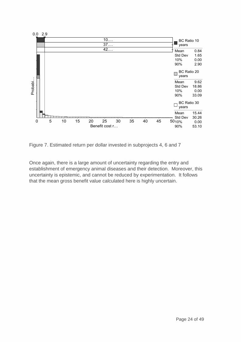
5.4.3. Benefit

Figure 6. Estimated benefit of subprojects 4, 6 and 7


Taking the mean of the distribution of model outputs shown in Figure 6 as our

estimate of the gross value of benefits generated by subprojects 4, 6 and 7, the

benefit cost ratio for the combined subprojects is approximately 15.4 over the 30

year period simulated. Distributions of benefit cost ratios produced by the model

are shown in Figure 7 for 10, 20 and 30-year time frames.

Note that while the subproject is expected to make a net loss over the first 10

years of the assessment, by the end of the 30-year period the return on

investment is likely to large (i.e. $15.44 returned for each $1.00 invested in these

subprojects). These returns are calculated on the basis of a single case study,

FMD.

The assumptions on the FMD simulation model is based are detailed in

Appendix 1, Table A3. By the end of the 30-year estimation period, subprojects

4, 6 and 7 are estimated to have a combined net present value of $106.3 million.

of 49

Figure 7. Estimated return per dollar invested in subprojects 4, 6 and 7

Once again, there is a large amount of uncertainty regarding the entry and

establishment of emergency animal diseases and their detection. Moreover, this

uncertainty is epistemic, and cannot be reduced by experimentation. It follows

that the mean gross benefit value calculated here is highly uncertain.

of 49

5.5. Subproject 5: Agricultural weed surveillance in the South West to

protect industry profitability

5.5.1. Background

Subproject 5 aims to develop enhanced weed surveillance methods for 20

declared weeds affecting intensive horticultural production in the South West

region.

Of the species targeted in the project, 15 are to be selected by DAFWA and 5 by

community stakeholders. Information concerning their abundance and

distribution in the region is to be collected and interpreted using DAFWA staff

expertise in cooperation with Recognised Biosecurity Groups.

Reporting methods and procedures for new and established species are to be

refined with the view to reducing the time between detection in an area and

response.

This is to be achieved primarily via the development of the MyWeedWatcher

smartphone app but may also involve drone technology. Weed damage

prevented will accrue over time and can be evaluated using a set of case study

species affected by the subproject.

5.5.2. Cost

This subproject involves a total investment of $1 159 000 and is 100% funded

through the RfR initiative.

5.5.3. Benefit


https://www.agric.wa.gov.au/myweedwatcher-information

of 49


Using the mean of the distribution of model outputs shown in Figure 8 as an

estimate of the gross value of the project, the benefit cost ratio for subproject 5 is

estimated to be 2.1 over the first decade of the subproject, and 38.0 by the end

of the third decade. At the end of the 30-year estimation period the subproject is

expected to have a net present value of approximately $33.16 million. The

assumptions on which this is based are detailed in Appendix 1, Table A4.

Distributions of benefit cost ratios produced by the model are shown in Figure 9

for 10, 20 and 30-year time frames. Note that the benefits include losses

prevented in regions outside of the South West in cases where weeds can

spread to warmer and drier regions.


of 49

5.6. Subproject 6: Build capacity to respond and recover from

emergency pest and disease incidents

5.6.1. Background

This subproject is designed to address crucial factors affecting the ability of the

agrifood sector in WA to recover following a biosecurity emergency response. It

comprises of eight separate components, which include:

A Training for 275 DAFWA staff emergency response management;

B Recovery component targeting communication with local government and

emergency management groups to raise community awareness regarding

biosecurity emergencies;

C Purchase and implementation of software programs to enhance (i)

interagency support and logistics management (Web EOC), and (ii)

incursion operations and planning (MAX);

D Supports DAFWA staff gaining experience with real incursions occurring

within Australia to enhance skills and performance in biosecurity emergency

situations;

E Improving laboratory management and cataloguing of field samples

collected in biosecurity emergencies;

F Training industry liaison officers to contribute local industry knowledge and

industry involvement in emergency responses;

G Planning for large scale destruction of livestock biomass as part of a state

or national ‘stamp out’ response policy;

H Supporting the FMD simulation exercise, APOLLO (2016).

5.6.2. Cost

This subproject involves a total investment of $5 650 000. Of this, $5 000 000 is

received from RfR funds, while the remainder if from DAFWA consolidated funds.

5.6.3. Benefit

Please see section 5.4.3. Parameters used in the assessment appear in

Appendix 1, Table A3.


The return on investment to this subproject is evaluated together with

subprojects 4 and 7. Please see section 5.4.4.

https://www.intermedix.com/solutions/webeoc

http://agriculture.vic.gov.au/about-us/media-centre/media-releases/maximum-points-for-biosecurity-software-innovation

https://www.agric.wa.gov.au/livestock-biosecurity/exercise-apollo-national-emergency-response-exercise

of 49

5.7. Subproject 7: Awareness and compliance with new biosecurity

legislation

5.7.1. Background

This subproject seeks to improve awareness of and compliance with the

Biosecurity and Agricultural Management Act 2007 (Parliament of Western

Australia, 2007), or BAM Act. It aims to do so via four activities:

A. Swill Feeding – Develop an education package for high-risk community

groups regarding swill feeding risks and risk management;

B. Sheep Traceability – Develop a communication plan to extend knowledge

of the National Livestock Identification System (NLIS) requirements to

sheep producers via a series of regional workshops and through the

creation of a sheep NLIS helpdesk;

C. Regulatory Training – Develop a tailored Certificate III in Government

course that includes units of competency focused on statutory compliance

for DAFWA officers appointed as inspectors under the BAM Act;

D. Work instructions/Procedural documents – Draft and distribute twenty

procedural documents to relevant DAFWA officers.

5.7.2. Cost

This subproject involves a total investment of $1 120 000. Of this, $120 000

represents DAFWA in-kind support, and $1 000 000 is received from the RfR

initiative.

5.7.3. Benefit

Please see section 5.4.3. Parameters used in the assessment appear in

Appendix 1, Table A3.


The return on investment to this subproject is evaluated together with

subprojects 4 and 6. Please see section 5.4.4.

https://www.animalhealthaustralia.com.au/what-we-do/biosecurity-services/national-livestock-identification-scheme/nlis-sheep-goats/

of 49

5.8. Subproject 8: Biosecurity research and development fund

5.8.1. Background

Subproject 8 makes $3 200 000 available to fund research projects developing

solutions to significant pests and diseases affecting WA. Grants of between

$50 000 and $500 000 per year will be offered over a three-year period

beginning 2015.

In the first round of funding, $2 500 000 from the Fund was distributed across

seven projects that successfully nominated for funds. Of these, the Goldfields

Nullarbor Rangelands Biosecurity Association (GNRBA) project entitled Using

innovative technologies to identify and map invasive cacti in the southern

Rangelands of WA is used as a case study.

The GNRBA project involves a $158 500 Fund investment to identify and map

invasive cacti in the southern Rangelands of WA. Species targeted include coral

cactus (Cylindropuntia fulgida), Hudson pear (C. rosea and C. tunicate) and

devil’s rope cactus (C. imbricata).

Four locations of 80ha were initially selected (Menzies, Mertondale, Coolgardie

and Tarmoola Station), but detailed mapping of cacti will now only be carried out

for the Coolgardie and Tarmoola Station sites. Large infestations in these areas

will be mapped using a near-infrared camera mounted to an unmanned aerial

vehicle, while ground-based thermal imaging technology will be used to identify

infestations obscured by shrub and woodland canopies.

Information generated by the project concerning the location and density of

infestations will lower the costs of control (i.e. via reduced search costs) and

more effective targeting of management effort. Benefits are only calculated for

the goldfields region despite the capacity for cacti to infest other regions.

5.8.2. Cost

Subproject 8 involves a total investment of $3 500 000 received from the RfR

initiative.

The GNRBA grant for the Using innovative technologies to identify and map

invasive cacti in the southern Rangelands of WA project involves a total

investment of $158 000.

http://www.gnrba.com.au/invasive-cacti.html



of 49

5.8.3. Benefit

Figure 10. Estimated benefit of Using innovative technologies to identify and map


subproject 8



estimate of the gross value of benefit generated, the benefit cost ratio for by the

Using innovative technologies to identify and map invasive cacti in the southern

Rangelands of WA project is estimated to be 2.4 by the end of the 30-year

estimation period. The net present value for the project is estimated as

$0.2 million. The assumptions on which this is based are detailed in Appendix 1,

Table A5.

Figure 11 shows the distributions of benefit cost ratios produced by the model for

10, 20 and 30-year estimation periods. The further in time benefits are projected,

the higher the returns on investment in the project.

of 49

Figure 11. Estimated return per dollar invested in the Using innovative

technologies to identify and map invasive cacti in the southern

Rangelands of WA project funded under subproject 8

of 49

5.9. Subproject 9: Transforming regional biosecurity response

5.9.1. Background

The focus of subproject 9 is established pest management and changing the

governance structure from a ‘top down’ government led approach to a ‘bottom

up’ community coordinated approach. This is in line with DAFWA’s adoption of

the National Framework for Management of Established Pests and Diseases of

National Significance via a community co-ordinated approach, with Recognised

Biosecurity Groups (RBGs) forming the basis of established invasive species

management.

5.9.2. Cost

This subproject involves a total investment of $3 308 000 from the RfR initiative

and a further $700 000 from the State Natural Resource Management Office.

5.9.3. Benefit

Not applicable.


Subproject 9 is not evaluated as part of this assessment.

However, with regard to the National Framework for Management of Established

Pests and Diseases of National Significance using the invasion impact curve

(Agriculture Victoria, 2015) as the basis for shifting the control of established

species from government to community, please see section 5.2.4.

http://www.agriculture.gov.au/SiteCollectionDocuments/biosecurity/framework-pests-diseases.pdf

http://www.agriculture.gov.au/SiteCollectionDocuments/biosecurity/framework-pests-diseases.pdf

of 49

5.10. Subproject 10: Eradication of Medfly in Carnarvon

5.10.1. Background

Subproject 10 aims to eradicate Mediterranean fruit fly (Ceratitis capitata, or

Medfly) from the Carnarvon horticulture precinct. This will lower the variable cost

of production for fruit and vegetables from the region.

Experience overseas (e.g. USA, Mexico and Chile) has shown that it is possible

to achieve Medfly eradication provided reintroduction events can be controlled

(Mumford et al., 2001). This subproject relies on the relative isolation of

Carnarvon enabling the ongoing exclusion of Medfly once eradication has been

achieved.

Restrictions on broad-spectrum organophosphorus insecticide use have

increased the significance of Medfly as pest of WA horticulture (APVMA, 2010,

Mengersen et al., 2012, Cook and Fraser, 2014). This is particularly true in

regional economies highly dependent on susceptible industries, such as

Carnarvon in the State’s midwest region. Here, agriculture contributes over $100

million to the regional economy (ABS, 2015).

5.10.2. Cost

This subproject involves a total investment of $4 200 000. This comprises of

$1 100 000 from the RfR initiative, $1 500 000 DAFWA in-kind funds, $1 000 000

from Horticulture Innovation Australia Ltd. and $600 000 from the Carnarvon

Grower Association.

5.10.3. Benefit


of 49



estimate of the gross value of benefit generated, the benefit cost ratio for the

eradication of Medfly from Carnarvon is estimated to be 3.4 by the end of the 30-

year estimation period. The net present value for the project is estimated to be

$7.47 million. As noted in the assumptions on which this assessment is based

(detailed in Appendix 1, Table A6), only a sub-sample of crops potentially

affected by the project have been included.

Figure 13 shows the distributions of benefit cost ratios produced by the model for

10, 20 and 30-year estimation periods. This figure shows that while short-term

returns to investment in the subproject are negative, they are healthy in the

medium to long term as the producer benefits of Medfly eradication accumulate.


of 49

5.11. Subproject 11: Wild dog control measures

5.11.1. Background

Subproject 11 will investigate the likely costs and benefits of different wild dog

management strategies, and how these affect WA rangeland livestock

production. The subproject will focus on southern rangeland areas in which the

Carnarvon, Meekatharra and Goldfields Recognised Biosecurity Groups operate,

and make a detailed study of interactions between wild dogs and livestock within

specific sites of interest. Control techniques to be explored include trapping,

ground and aerial baiting, professional hunters and trappers, bounties and

exclusion fencing.

5.11.2. Cost

This subproject involves a total investment of $671 000, comprising of $596 000

from the RfR initiative and $75 000 from DAFWA.

5.11.3. Benefit

Not applicable.


Subproject 11 is not evaluated as part of this assessment.

of 49

5.12. Synthesis

Using the individual assessments of sections 5.1 to 5.11 in an aggregated

assessment of the BBD project is very difficult. Ideally, we would run all 20 pest

and disease simulations simultaneously. However, using such a large ensemble

of creates a great deal of model instability. Computationally, when we consider

many of the species involved are polyphagous pests and diseases (i.e. spread

occurs in a number of different crops for each species), simulating their

movement across all crops over a 30-year period is extremely complicated.

To enable the aggregation of subproject results, distributions were fitted to

subproject model outputs, and these fitted distributions were then used to

represent individual species benefits generated by the project in a separate

model.

Unfortunately, this aggregated model is aspatial, which means there is an

element of double counting in the calculations. If, for example, multiple pest and

disease outbreaks occur in one single year affecting a common crop, our method

of aggregating project benefits does not account for overlapping damages.

Keeping in mind this upward bias, the net impact of the project is seen in

Figure 14. Here, the distributions of net present value for the BBD project in the

aggregated model is shown for 10, 20 and 30-year estimation periods. From an

initial net loss of $0.8 million over the first 10 years, the project is expected to

post net benefits of approximately $241.9 million by year 30.

Figure 14. Distribution of simulated pest and disease impacts with and without

the BBD project

of 49

Distributions of benefit cost ratios expected from the project are shown in

Figure 15. As with Figure 14, separate distributions are displayed for 10, 20 and

30-year estimation periods. The influence of time on results can be seen in the

description of the three distributions on the right-hand-side of the figure. The

mean benefit cost ratio increases from 1.0 to 17.4 as we increase the time period

from 10 years to 30 years. This is despite the erosive effects of the discount

rate.

Figure 15. Estimated return on investment from the BBD project

Returns on investment in the project increase with time as the benefits of pest

and disease damages prevented accumulate. As the costs of the project cease

beyond 2017, the longer the length of time over which we calculate the benefits

the larger those benefits are relative to costs.

This is further revealed in Table 3 in which the present (or discounted) value of

benefits, present value of costs, net present value and benefit cost ratio are

shown for the 10, 20 and 30-year time frames. All costs are incurred within the

10-year time frame, while benefits accrue over the 20 and 30-year periods.

of 49

Table 3. Estimated return on investment from the Boosting Biosecurity Defences

project over time

10 years 20 years 30 years

Present value of benefits ($M) 14.00 159.96 256.65

Present value of costs ($M) 14.76 14.76 14.76

Net present value ($M) -0.76 145.20 241.89

Benefit cost ratio 0.95 10.84 17.39

Figure 8 and Table 3 reveal returns on investment in the project to be large over

the medium (≈ 20-year) and long (≈ 30-year) term using the set of case studies

outlined in sections 5.1 to 5.11, but are small in the short term (≈ 10 years).

Returns grow over time as a result of the initial investment reducing future

damage. This makes the choice of time frame critical when assessing the

relative success of the project.

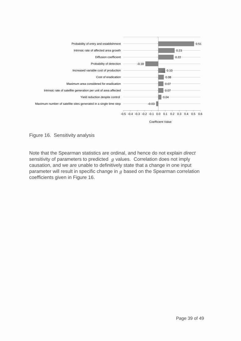
In view of the uncertainty surrounding parameters describing invasive species

arrival and spread processes in the model, the sensitivity of gross benefit

calculations (i.e. 𝑔, recalling Eq. 7) to key assumptions must be tested to gauge

the robustness of predictions. Parameters were sampled from a uniform

distribution with a maximum (minimum) of +50 per cent (-50 per cent) of the

original values entered in to the model using Monte Carlo simulation. The

Spearman’s rank correlation coefficients relating the sampled model parameter

values and changes in 𝑔 were then calculated.

The numerical value of the Spearman’s rank correlation coefficient is denoted ,

where -1.0 ≤ ≤ 1.0. If 𝑔 has a tendency to increase when a parameter

increases is positive, and vice versa. A value of zero indicates that there is

no tendency for 𝑔 to increase or decrease, while a of one indicates that they

are perfect monotone functions of each other. Parameters and their values are

presented in Figure 16.

The sensitivity tests indicate that 𝑔 is most responsive in simulations involving

exotic invasive species threats. Changes in the probability of entry and

establishment produce the largest sensitivity (i.e. value of 0.51). Results are

also responsive to the intrinsic rate of affected area growth (0.23), the population

diffusion coefficient (0.22), the probability of detection (-0.18) and the increased

variable cost of production (0.10).

of 49

0.51

0.23

0.22

-0.18

0.10

0.08

0.07

0.07

0.04

-0.03

-0.5 -0.4 -0.3 -0.2 -0.1 0.0 0.1 0.2 0.3 0.4 0.5 0.6

Probability of entry and establishment

Intrinsic rate of affected area growth

Diffusion coefficient

Probability of detection

Increased variable cost of production

Cost of eradication

Maximum area considered for eradication

Intrinsic rate of satellite generation per unit of area affected

Yield reduction despite control

Maximum number of satellite sites generated in a single time step

Coefficient Value

Figure 16. Sensitivity analysis

Note that the Spearman statistics are ordinal, and hence do not explain direct

sensitivity of parameters to predicted 𝑔 values. Correlation does not imply

causation, and we are unable to definitively state that a change in one input

parameter will result in specific change in 𝑔 based on the Spearman correlation

coefficients given in Figure 16.

of 49

6. Conclusion

This report has used a bioeconomic model to estimate the likely returns to

investment in BBD subprojects over a 30-year period. The model estimates the

reduction in expected pest and disease damage with each subproject compared

to without it. This prevented damage constitutes the benefits of the subprojects,

which are then compared to the costs of each t provide a benefit cost analysis.

Results for each subproject are as follows. Note that results assume BBD

subprojects achieve their intended outcomes:

Subproject 1: State Biosecurity Strategy is not included in the assessment

due to the general, non-specific nature of benefits flowing from the project;

Subproject 2: E-Surveillance for pests and diseases in the WA grains industry

is estimated to produce $22.77 for every $1.00 invested;

Subproject 3: E-Surveillance for pests and diseases of the WA grape industry

is estimated to produce $56.40 for every $1.00 invested;

Subprojects 4, 6 and 7: Early detection of emergency animal diseases,

Capacity to Respond and Recover and Awareness and compliance with new

biosecurity legislation, respectively, are estimated to be produce a combined

$15.44 for every $1.00 invested. Due to time constraints, this is only

evaluated on the basis of a single animal disease case study (foot-and-mouth

disease);

Subproject 5: Agricultural weed surveillance in the South West to protect

industry profitability is estimated to produce $38.03 for every $1.00 invested;

Subproject 8: Biosecurity research and development fund is estimated to

produce $2.44 for every $1.00 invested. Due to time constraints, this is only

evaluated on the basis of a single case study (Using innovative technologies

to identify and map invasive cacti in the southern Rangelands of WA);

Subproject 9: Transforming regional biosecurity response is not included in

the assessment;

Subproject 10: Eradication of Medfly in Carnarvon is estimated to produce

$3.38 for every $1.00 invested;

Subproject 11: Wild dog control measures is not included in the assessment.

Aggregating these subproject assessments, it is estimated that a net benefit of

$241.9 million will be created for the WA agricultural sector as a result of the

BBD project over a period of 30 years. These results are sensitive to changes in

several uncertain model parameters, including the probabilities of exotic species’

entry and establishment, the likelihood of detection and various spread

parameters.

of 49

7. References

ABS 2015. Value of Agricultural Commodities Produced, Australia, 2013-14, Canberra,

Australian Bureau of Statistics.

AGRICULTURE VICTORIA 2015. Invasive Plants and Animals Policy Framework,

Melbourne, Agriclture Victoria.

ANDOW, D. A., KAREIVA, P., LEVIN, S. A. & OKUBO, A. 1990. Spread of invading

organisms. Landscape Ecology, 4, 177-188.

APVMA 2010. Human Health Risk Assessment of Dimethoate, Canberra, Australian

Pesticides and Veterinary Medicines Authority.

COMMONWEALTH OF AUSTRALIA 2006. Handbook of Cost-Benefit Analysis,

Canberra, Department of Finance and Administration.

COOK, D., LIU, S., EDWARDS, J., VILLALTA, O., AURAMBOUT, J.-P., KRITICOS, D.,

DRENTH, A. & DE BARRO, P. 2013a. An assessment of the benefits of yellow

Sigatoka (Mycosphaerella musicola) control in the Queensland Northern Banana

Pest Quarantine Area. NeoBiota, 18, 67-81.

COOK, D., LONG, G., POSSINGHAM, H., FAILING, L., BURGMAN, M., GREGORY, R.,

ESTEVEZ, R. & WALSHE, T. 2010. Potential methods and tools for estimating

biosecurity consequences for primary production, amenity, and the environment.

Melbourne: Australian Centre of Excellence for Risk Analysis.

COOK, D. C. 2003. Prioritising Exotic Pest Threats to Western Australian Plant

Industries. Discussion Paper. Bunbury: Government of Western Australia -

Department of Agriculture.

COOK, D. C. 2008. Benefit cost analysis of an import access request. Food Policy, 33,

277–285.

COOK, D. C. 2011. Economic Impact Assessment Using a Partial Budgeting Approach:

Grapevine Phylloxera and Pierce’s Disease, Bunbury, Department of Agriculture

and Food, Western Australia.

COOK, D. C. 2015. Impact Assessments for Pests and Diseases Threatening the

Western Australia Grains Industry, Bunbury, Department of Agriculture and

Food, Western Australia.

COOK, D. C., CARRASCO, L. R., PAINI, D. R. & FRASER, R. W. 2011a. Estimating the

social welfare effects of New Zealand apple imports. Australian Journal of

Agricultural and Resource Economics, 55, 1-22.

COOK, D. C. & FRASER, R. W. 2014. Eradication versus control of Mediterranean fruit

fly in Western Australia. Agricultural and Forest Entomology, 17, 173-180.

COOK, D. C., FRASER, R. W., PAINI, D. R., WARDEN, A. C., LONSDALE, W. M. &

BARRO, P. J. D. 2011b. Biosecurity and yield improvement technologies are

strategic complements in the fight against food insecurity. PLoS ONE, 6, e26084.

of 49

COOK, D. C., LIU, S., EDWARDS, J., VILLALTA, O. N., AURAMBOUT, J.-P.,

KRITICOS, D. J., DRENTH, A. & DE BARRO, P. J. 2013b. Predicted economic

impact of black Sigatoka on the Australian banana industry. Crop Protection, 51,

48-56.

COUSINS, D. 2015. Draft Project Plan: Royaltiesfor Regions - Boosting WA’s

Biosecurity Defences (A557088), South Perth, Department of Agriculture and

Food, Western Australia.

DWYER, G. 1992. On the spatial spread of insect pathogens - theory and experiment.

Ecology, 73, 479-494.

GARNER, M. G. & BECKETT, S. D. 2005. Modelling the spread of foot-and-mouth

disease in Australia. Australian Veterinary Journal, 83, 758-766.

HENGEVELD, B. 1989. Dynamics of Biological Invasions, London, Chapman and Hall.

HOLMES, E. E. 1993. Are diffusion-models too simple - a comparison with telegraph

models of invasion. American Naturalist, 142, 779-795.

HOOPER, G. H. S. & DREW, R. A. I. 1989. Australia and South Pacific Islands. In:

ROBINSON, A. S., HOOPER, G.H.S. (ed.) Fruit Flies: Their Biology, Natural

Enemies and Control. Amsterdam: Elsevier.

LEWIS, M. A. 1997. Variability, patchiness, and jump dispersal in the spread of an

invading population. In: TILMAN, D. & KAREIVA, P. (eds.) Spatial Ecology: The

Role of Space in Population Dynamics and Interspecific Interactions. New

Jersey: Princeton University Press.

LYYTINEN, K. & DAMSGAARD, J. 2001. What’s Wrong with the Diffusion of Innovation

Theory? In: ARDIS, M. A. & MARCOLIN, B. L. (eds.) Diffusing Software Product

and Process Innovations: IFIP TC8 WG8.6 Fourth Working Conference on

Diffusing Software Product and Process Innovations April 7–10, 2001, Banff,

Canada. Boston, MA: Springer US.

MCCANN, K., HASTINGS, A., HARRISON, S. & WILSON, W. 2000. Population

outbreaks in a discrete world. Theoretical Population Biology, 57, 97-108.

MENGERSEN, K., QUINLAN, M. M., WHITTLE, P. J. L., KNIGHT, J. D., MUMFORD, J.

D., WAN ISMAIL, W. N., TAHIR, H., HOLT, J., LEACH, A. W., JOHNSON, S.,

SIVAPRAGASAM, A., LUM, K. Y., SUE, M. J., OTHMAN, Y., JUMAIYAH, L., TU,

D. M., ANH, N. T., PRADYABUMRUNG, T., SALYAPONGSE, C., MARASIGAN,

L. Q., PALACPAC, M. B., DULCE, L., PANGANIBAN, G. G. F., SORIANO, T. L.,

CARANDANG, E. & HERMAWAN 2012. Beyond compliance: project on an

integrated systems approach for pest risk management in South East Asia.

EPPO Bulletin, 42, 109-116.

MOODY, M. E. & MACK, R. N. 1988. Controlling the spread of plant invasions: the

importance of nascent foci. Journal of Applied Ecology, 25, 1009-1021.

OKUBO, A. & LEVIN, S. A. 2002. Diffusion and ecological problems: modern

perspectives, New York, Springer.

of 49

PARLIAMENT OF WESTERN AUSTRALIA 2007. Biosecurity and Agriculture

Management Act 2007. Western Australia: Department of Premier and Cabinet,

State Law Publisher.

RICCIARDI, A. & COHEN, J. 2007. The invasiveness of an introduced species does not

predict its impact. Biological Invasions, 9, 309-315.

ROGERS, E. M. 2010. Diffusion of innovations, New York, Simon and Schuster.

ROGERS, E. M., MEDINA, U. E., RIVERA, M. A. & WILEY, C. J. 2005. Complex

adaptive systems and the diffusion of innovations. The Innovation Journal: The

Public Sector Innovation Journal, 10, 1-26.

SHIGESADA, N. & KAWASAKI, K. 1997. Biological Invasions: Theory and Practice,

Oxford, Oxford University Press.

WAAGE, J. K., FRASER, R. W., MUMFORD, J. D., COOK, D. C. & WILBY, A. 2005. A

New Agenda for Biosecurity Horizon Scanning Programme. London: Department

for Food, Environment and Rural Affairs.

of 49

8. Appendix

Table A1. Parameter values: Subproject 2 – E-Surveillance for pests and

diseases in the WA grains industry

Description With scenario* Without scenario

Cost of eradication, E

($/ha).

Khapra beetle Uniform(1.0106,1.0107)

Karnal bunt Uniform(1.0106,1.0107)

Cabbage Seedpod Weevil Uniform(5.0105,1.0106)

Ug99 Uniform(1.0106,1.0107)

Wheat stem sawfly Uniform(1.0106,1.0107)

Same as With scenario (")

Increased variable cost of

production, V ($/ha).


Karnal bunt 0

Cabbage Seedpod Weevil 0

Ug99 Discrete[(0.0,13.5,27.0)(0.5,1.0,1.0)]

Wheat stem sawfly Uniform(3,5)

"

Intrinsic rate of affected

area growth, r (wk-1).

Khapra beetle Pert(0.20,0.35,0.50)

Karnal bunt Pert(1,2,3)

Cabbage Seedpod Weevil Pert(0.20,0.35,0.50)

Ug99 Pert(1.0,1.25,1.5)

Russian wheat aphid Pert(0.20,0.35,0.50)

"

Intrinsic rate of satellite

generation per unit of

area affected,

µ (#/ha).

Khapra beetle Pert(5.010-2,7.510-2,1.010-1)

Karnal bunt Pert(1.010-2,2.510-2,5.010-2)

Cabbage Seedpod Weevil Pert(1.010-3,5.510-3,1.010-2)

Ug99 Pert(1.010-2,2.510-2,5.010-2)

Wheat stem sawfly Pert(5.010-2,7.510-2,1.010-1)

"

Maximum area affected,

Amax (ha).

Khapra beetle 6.0106

Karnal bunt 4.7106

Cabbage Seedpod Weevil 1.1106

Ug99 4.7106

Wheat stem sawfly 3.5106

"

Maximum area considered

for eradication, Aerad

(ha)


Karnal bunt Pert(5.0103,7.5103,1.5104)


Ug99 Pert(5.0103,7.5103,1.5103)

Wheat stem sawfly Pert(5.0103,7.5103,1.5103)

"

Maximum density, K (#/ha).



Cabbage Seedpod Weevil Uniform(1.0103,1.0104)

Ug99 Uniform(1.0102,1.0103)

Wheat stem sawfly Uniform(1.0104,1.0105)

"

Maximum number of

satellite sites

generated in a single

time step, smax (#).

Khapra beetle Pert(30,40,50)


Cabbage Seedpod Weevil Pert(10,15,20)

Ug99 Pert(70,85,100)

Wheat stem sawfly Pert(30,40,50)

Khapra beetle Pert(10,15,20)

Karnal bunt Pert(5.0,7.5,10.0)


Ug99 Pert(30,40,50)


Minimum density, Nmin

(#/ha).




Ug99 1.0×10-8

Wheat stem sawfly Pert(0.00,0.025,0.050)


Diffusion coefficient, D

(ha/wk).



Cabbage Seedpod Weevil Pert(2,3,4)

Ug99 Pert(4,6,8)


"

Prevailing price for affected

commodities, P ($/T).

Barley 213

Canola 542

Wheat 280

Oats 176

"

Probability of detection, (%)

Khapra beetle binomial(1.0,0.4)

Karnal bunt binomial(1.0,0.4)

Cabbage Seedpod Weevil binomial(1.0,0.4)

Ug99 binomial(1.0,0.4)

Wheat stem sawfly binomial(1.0,0.4)

Khapra beetle binomial(1.0,0.8)

Karnal bunt binomial(1.0,0.8)

Cabbage Seedpod Weevil binomial(1.0,0.8)

Ug99 binomial(1.0,0.8)

Wheat stem sawfly binomial(1.0,0.8)

Yield reduction despite

control, Y (%).

Barley Uniform(0,20)

Canola Uniform(0,20)

Wheat Uniform(0,20)

Oats Uniform(0,20)

Same as With scenario

* Cook (2015) and Cook et al. (2011b).

of 49

Table A2. Parameter values: Subproject 3 – E-Surveillance for pests and

diseases of the WA grape industry



($/ha).

Pierce’s disease Uniform(1.0106,1.0107)

Grapevine phylloxera 3.0104

Brown marmorated stink bug Uniform(5.0105,1.0106)

Grapevine fanleaf virus Uniform(1.0106,1.0107)

Grapevine leaf rust Uniform(1.0106,1.0107)




Pierce’s disease Discrete[(0,40,80,120)(1,1,1,1)]

Grapevine phylloxera Pert(2.0104, 3.0104, 4.0104)

Brown marmorated stink bug Discrete[(0,10,20,30)(1,1,1,1)]

Grapevine fanleaf virus 725

Grapevine leaf rust 725

"



Pierce’s disease Pert(0.20,0.35,0.50)

Grapevine phylloxera Pert(0.10,0.15,0.20)

Brown marmorated stink bug Pert(0.20,0.35,0.50)

Grapevine fanleaf virus Pert(1.0,1.25,1.5)

Grapevine leaf rust Pert(0.20,0.35,0.50)

"



area affected,

µ (#/ha).

Pierce’s disease Pert(5.010-2,7.510-2,1.010-2)

Grapevine phylloxera Uniform(1.010-3,1.010-2)

Brown marmorated stink bug Pert(1.010-2, 2.510-2,5.010-2)

Grapevine fanleaf virus Pert(1.010-2,2.510-2,5.010-2)

Grapevine leaf rust Pert(5.010-2,7.510-2,1.010-1)

"


Amax (ha).

Pierce’s disease 1.1104

Grapevine phylloxera 5.5103

Brown marmorated stink bug 1.1104

Grapevine fanleaf virus 1.1104

Grapevine leaf rust 1.1104

"



(ha)






"


Pierce’s disease Uniform(1.0104,1.0105)

Grapevine phylloxera Uniform(1.0103,1.0104)

Brown marmorated stink bug Uniform(1.0103,1.0104)

Grapevine fanleaf virus Uniform(1.0102,1.0103)

Grapevine leaf rust Uniform(1.0104,1.0105)

"

Maximum number of

satellite sites



Pierce’s disease Pert(30,40,50)

Grapevine phylloxera Pert(10,15,20)

Brown marmorated stink bug Pert(50,60,70)

Grapevine fanleaf virus Pert(30,40,50)

Grapevine leaf rust Pert(50,60,70)

Pierce’s disease Pert(10,15,20)


Brown marmorated stink bug Pert(30,40,50)

Grapevine fanleaf virus Pert(10,15,20)

Grapevine leaf rust Pert(30,40,50)


(#/ha).




Grapevine fanleaf virus Pert(0.00,0.025,0.050) Grapevine

leaf rust Pert(0.00,0.025,0.050)



(ha/wk).






"


commodities, P ($/T). Grapes 1430 "


Pierce’s disease binomial(1.0,0.6)

Grapevine phylloxera binomial(1.0,0.6)

Brown marmorated stink bug binomial(1.0,0.6)

Grapevine fanleaf virus binomial(1.0,0.6)

Grapevine leaf rust binomial(1.0,0.6)

Pierce’s disease binomial(1.0,0.8)

Grapevine phylloxera binomial(1.0,0.8)

Brown marmorated stink bug binomial(1.0,0.8)

Grapevine fanleaf virus binomial(1.0,0.8)

Grapevine leaf rust binomial(1.0,0.8)


control, Y (%). Grapes Uniform(0,10) Same as With scenario

* Cook (2003) and Cook (2011).

of 49

Table A3. Parameter values: Subproject 4 – Early detection of emergency animal

diseases; Subproject 6 – Build capacity to respond and recover from

emergency pest and disease incidents; and Subproject 7 – Awareness

and compliance with new biosecurity legislation



($/ha). FMD Uniform(20,000,000.0107,4.0107) Uniform(1.8107,3.6107)


production, V ($/hd). FMD 15 Same as With scenario (")


area growth, r (wk-1). FMD Pert(1.50,1.75,2.00) "



area affected,

µ (#/hd).

FMD Pert(0.10,0.15,0.20) "

Maximum population

affected, Amax (hd). FMD 5.4107 "

Maximum population

considered for

eradication, Aerad

(hd).

FMD Pert(5.0103,7.5103,1.5103) "

Maximum density, K (#/hd). FMD Uniform(1.0106,1.0107) "

Maximum number of

satellite sites



FMD Pert(50,60,70) "


(#/hd). FMD Pert(0.00,0.025,0.050) "


(hd/wk). FMD Pert(14,18,22) "


commodities, P

(c/kg).

Cattle and calves 550

Milk 250

Pigs and pig meat 400

Sheep and lamb 550

"

Probability of (re-)entry and

establishment (%). FMD Uniform(3.010-5,7.010-2 "

Probability of detection,

(%). FMD binomial(1.0,0.7) FMD binomial(1.0,0.6)

Reduction in export

earnings attributable

to a loss of

pest/disease area

freedom (%)

FMD Pert(70,85,100) Same as With scenario (")


control, Y (%). FMD Uniform(0,30) "

* Waage et al. (2005). Note that the probability of FMD’s entry and establishment in WA is considered relatively low.

This has the effect of lowering the ‘expected’ gross benefits of subprojects 4,6 and 7.

of 49

Table A4. Parameter values: Subproject 5 – Agricultural weed surveillance in the

South West to protect industry profitability


Cost of eradication, E ($/ha).

Jointed goatgrass Uniform(1.0103,1.5103)

Branched broomrape Uniform(1.0103,1.5103)

Hoary cress Uniform(1.0103,1.5103)

Creeping knapweed Uniform(1.0103,1.5103)

Golden dodder Uniform(1.0103,1.5103)





Branched broomrape Uniform(50,150)

Hoary cress Uniform(15,30)

Creeping knapweed Uniform(15,30)

Golden dodder Uniform(50,150)

"

Intrinsic rate of affected area

growth, r (wk-1).


Branched broomrape Pert(1,2,3)

Hoary cress Pert(0.50,0.75,1.00)

Creeping knapweed Pert(1.0,1.25,1.5)

Golden dodder Pert(0.20,0.35,0.50)

"



area affected, µ (#/ha).

Jointed goatgrass Pert(5.010-2,7.510-2,1.010-1)

Branched broomrape Pert(5.010-2,7.510-2,1.010-1)

Hoary cress Pert(1.010-3,5.510-3,1.010-2)

Creeping knapweed Pert(1.010-2,2.510-2,5.010-2)

Golden dodder Pert(5.010-2,7.510-2,1.010-1)

"

Maximum area affected, Amax

(ha).

Jointed goatgrass 4.6106

Branched broomrape 1.1106

Hoary cress 1.0106

Creeping knapweed 4.7106

Golden dodder 2.0103

"

Maximum area considered for

eradication, Aerad (ha)

Jointed goatgrass Uniform(500,1000)

Branched broomrape Uniform(500,1000)

Hoary cress Uniform(500,1000)

Creeping knapweed Uniform(500,1000)

Golden dodder Uniform(500,1000)

"



Branched broomrape Uniform(1.0104,1.0105)

Hoary cress Uniform(1.0103,1.0104)

Creeping knapweed Uniform(1.0103,1.0104)

Golden dodder Uniform(1.0104,1.0105)

"

Maximum number of satellite

sites generated in a

single time step, smax

(#).

Jointed goatgrass Pert(30,40,50)


Hoary cress Pert(10,15,20)

Creeping knapweed Pert(70,85,100)

Golden dodder Pert(30,40,50)

"

Minimum density, Nmin (#/ha).

Jointed goatgrass Pert(1,2,3)





"


(ha/wk).

Jointed goatgrass Pert(1.0,1.5,2.0)





"



Barley 213

Canola 542

Carrot 750

Oats 176

Onion 900

Potato 750

Tomato 1800

Wheat 280

"


Jointed goatgrass binomial(1.0,0.4)

Branched broomrape binomial(1.0,0.4)

Hoary cress binomial(1.0,0.4)

Creeping knapweed binomial(1.0,0.4)

Golden dodder binomial(1.0,0.4)

Jointed goatgrass binomial(1.0,0.6)

Branched broomrape binomial(1.0,0.6)

Hoary cress binomial(1.0,0.6)

Creeping knapweed binomial(1.0,0.6)

Golden dodder binomial(1.0,0.6)


control, Y (%).

Barley Uniform(0.0,0.1)

Canola Uniform(0.0,0.1)

Carrot Uniform(0.0,1.0)

Lupins Uniform(0.0,0.1)

Oats Uniform(0.0,0.1)

Onion Uniform(0.0,1.0)

Potato Uniform(0.0,1.0)

Tomato Uniform(0.0,1.0)

Wheat Uniform(0.0,0.1)

Same as With scenario


of 49

Table A5. Parameter values: Using innovative technologies to identify and map


subproject 8



($/ha).

Coral cactus Uniform(300,500)

Hudson pear Uniform(300,500)

Devil’s rope cactus Uniform(300,500)






Coral cactus Discrete({100,200,300}{1,1,0.5})

Hudson pear Discrete({100,200,300}{1,1,0.5})

Devil’s rope cactus Discrete({100,200,300}{1,1,0.5})




Coral cactus Pert(0.20,0.35,0.50)

Hudson pear Pert(0.20,0.35,0.50)

Devil’s rope cactus Pert(0.20,0.35,0.50)

"



area affected,

µ (#/ha).

Coral cactus Pert(1.010-5,6.010-4,1.010-3)

Hudson pear Pert(1.010-5,6.010-4,1.010-3)

Devil’s rope cactus Pert(1.010-5,6.010-4,1.010-3)

"


Amax (ha).

Coral cactus 7.71011

Hudson pear 7.71011

Devil’s rope cactus 7.71011

"



(ha)

Coral cactus Pert(5.0106, 7.5106,1.0107)

Hudson pear Pert(5.0106, 7.5106,1.0107)

Devil’s rope cactus Pert(5.0106, 7.5106,1.0107)

"



Hudson pear Pert(1.0104,5.5104,1.0105)


"

Maximum number of

satellite sites






"


(#/ha).

Coral cactus 1.010-4

Hudson pear 1.010-4

Devil’s rope cactus 1.010-4

"


(ha/wk).


Hudson pear Pert(5.0103,6.25103,7.5103)


"


commodities, P

($/kg).

Beef 1.75

Wool 7.09 "


Coral cactus Binomial(100,0.8)

Hudson pear Binomial(100,0.8)

Devil’s rope cactus Binomial(100,0.8)

Coral cactus Binomial(100,0.4)

Hudson pear Binomial(100,0.4)

Devil’s rope cactus Binomial(100,0.4)


control, Y (%).

Beef Uniform(0.0,2.0)

Wool Uniform(0.0,2.0) Same as With scenario


of 49

Table A6. Parameter values: Subproject 10 – Eradication of Medfly from

Carnarvon



($/ha). Pert(2.0104,3.0104,4.0104) 0


production, V ($/ha). Pert(50,100,150) Same as With scenario (")


area growth, r (wk-1). Pert(0.20,0.35,0.50) "



area affected,

µ (#/ha).

Pert(1.010-2,3.010-2,5.010-2) "


Amax (ha).

Citrus 1440

Mango 840

Stone 600

Table grapes 240

Tomato 390

"



(ha)

3,500 0

Maximum density, K (#/ha). Pert(100,550,1000) Same as With scenario (")

Maximum number of

satellite sites



Pert(50,60,70) "


(#/ha). Pert(1,2,3) "


(ha/wk). Pert(5.0105,6.0105,7.0105) "



Citrus 2000

Mango 5000

Stone 1500

Table grapes 2500

Tomato 1800

"

Probability of detection, (%) na Binomial(1.0,0.6)


control, Y (%). Pert(2.0,3.5,5.0) Same as With scenario

* Cook and Fraser (2014). Note that only a small sub-sample of crops influenced by the project are included in the

assessment. Medfly is known to affect most commercial fruit crops and over 60 native fruit species (Hooper and Drew,

1989), but given restrictions in the stochastic model used in this assessment it is not possible to include all potentially-

affected crops.

Benefit Cost Analysis

Documents

Transcript of Benefit Cost Analysis