Bending Vibration of Rotating Drill Strings
145
Bending Vibration of Rotating Drill Strings by Shyu rJ. S., Nat i () naI eng -I( II ng l Jn i vf' rs i t y, 'ra ina ll, '1' a i \va II ( 1980) 1\1. S., National 'l'ai\van lJnivcrsity, 'raipei, 'raiv,ian (1982) Sllbnlitted in Partial FIIlfilJlrlent of tile R.eqllirelnents for Degree of Doctor of Pllilosophy in Ocean at the Massachusetts Institute of Technology August 1989 ©l\1assachusetts Institute of Technology, 1989 Signature of Author _ of Ocpan A llgllSt. 7, J DHD C;crtificd by . V_V-.........""_F........ '-V_.V_""""_-_-_· _ / })rofcssor .1. KiTTl Vandiver Thesis Supervisor :I MASSACHUSEnS INSTil l JTE Of TfC!-J'.· ;¥ A ccepted by __ __ ,-- -=<::::::J Professor A. Douglas Carmichael Chairman, Departmental Graduate Comrnittee 0 V 17 1989
Transcript of Bending Vibration of Rotating Drill Strings

Bending Vibration of Rotating Drill Strings
by
I~.ong-Juin Shyu
rJ. S., Nat i() na I (~heng-I( II ng l Jn ivf' rs i t y, 'raina ll, '1'a i \va II
( 1980)
1\1. S., National 'l'ai\van lJnivcrsity, 'raipei, 'raiv,ian
(1982)
Sllbnlitted in Partial FIIlfilJlrlent
of tile R.eqllirelnents for tll~
Degree of
Doctor of Pllilosophy
in Ocean Erlgin(~ering
at the
Massachusetts Institute of Technology
August 1989
©l\1assachusetts Institute of Technology, 1989
Signature of Author _
D(~partment of Ocpan 11:n~iTlcerillg
A llgllSt. 7, JDHD
C;crtificd by . V_V-.........""_F........'-V_.V_""""_-_-_· _
/ })rofcssor .1. KiTTl Vandiver
Thesis Supervisor: I
MASSACHUSEnS INSTil l JTEOf TfC!-J'.· ;¥
Accepted by ---.L.._--'IIIl..c==~---=:::.sllL.____~-===___~--+'----_--,-- -=<::::::J
Professor A. Douglas Carmichael
Chairman, Departmental Graduate Comrnittee
,.~ 0V 17 1989

Bending Vibration of Rotating Drill Strings
by
Rong-Juin Shyu
Submitted to theDepartment of Ocean Engineering
un August 4, 1989 in partial fulfillment of the requirementsfor the Degree of Doctor of Philosophy
Abstl"act
Several domirlant mechanisms which cause the bending vibration of rotating drill
strings have been identified, they a.re :
• Linear coupling between d}"namic axial force and bending vibration
• Parametrically excited bending vibration due to dynamic axial force
• Whirling of the drill string with and without borehole contact
Mathematical models for explaining and predicting these bending behaviors have
been found and discussed. Experiments carried out in the laboratory confirmed tIle
existence of the linear and parametric coupling between axial force and bending vibration. Data from a field test conducted in 1984 by Shell Oil Company also showed
the existence of the both types of coupling. Forward and backward whirling of thedrill string are also evident in this data set.
Because of the effect of rotation, the frequencies needed to excite the linearlycoupled bending vibrations, and the parametrically excited bending vibration, arevarying linearly with respect to the rotational speed. This phenomenon is explained
and demonstrated by the laLoratory experiments. The effect of rotation plays a crucialrole in understanding the bending vibration of a rotating drill string.
Thesis Supervisor: Professor J. Kim Vandiver
Title: Professor of Ocean Engineering
2

Acknowledgments
I would, first of all, like to thank my academic and thesis advisor, Prof. J. Kim
Vandiver, for his helpful insights that lead me to this thesis topic, for his patience and
guidance that made this thesis possible, and for his great personality that made my
stay in MIT very fruitful and enjoyable. I would like to thank my thesis committee:
Prof. Stephen Crandall, Prof. Dale Karr, and Dr. George Triantafyllou, for their
critical suggestions that help in writing this thesis.
My special thanks go to my family, especially my parents, for their continuing
encouragement and support over the years. I would also like to thank my colleagues
over the years, C. Y. Liou, T. Y. Chung, N. Joglekar, H. Y. Lee, C. Y. Hsin, Chifang
Chen, H. Miyachi, for their numerous discussions and friendship. I would also like to
thank Ms. Shiela McNary for her many typing jobs.
This work is primarily sponsored by Agip, Amoco, Annadrill, Britoil-BritiGh Petroleum,
Elf Aquitaine, Exploration Logging, Exxon, Shell, Statoil, Teleco, and Total. A spe-
cial thanks goes to Shell Development Co. for the permission to publish data which
were acquired during a field test in 1984.
Finally, my thanks goes to two special friends r my master's thesis advisor, Prof.
C. S. Lee of National Taiwan University, and Ms. Chou Su, for their friendship and
encouragement which have positively changed many aspects of my life.
3

30
1818
19
24
Contents
1 Introduction 11
1.1 Basic Drilling Equipment 121.2 Problems in Drilling Dynamics 141.3 Outline of the Thesis . 15
2 Measurement Systems on a Rotating Shaft2.1 Motion of a Drill Collar in Pure Whirling .
2.2 Motion Seen From Coordinate Oxy .2.3 Motion Seen From the Rotating Coordinate System Ox'y'
2.4 Measurements Taken in a Rotating Reference Frame Under Pure Whirl
Condition ..... · . . . . . . . . . . . . . . . . . . . . . . . . . . .. 25
2.4.1 Bending ~1oments B r , and B II , •••••••••••••••••• 25
2.4.2 Acceleration ~1easurementswith Radial and Tangentially Mounted
Accelerometers Fixed to the Collar at a Radius Rs . . . . . .. 29
2.5 Measurements Taken on a Rotating Frame With Simultaneous Whirling
and Bending Vibration . . . . . . . . . . . . . . . . . . . . . . .
3 The Bending Natural Frequencies of Rotating Drill Collars3.1 Basic Configurations of the BHi\ .3.2 Theoretical Background .3.3 Added Mass Coefficient of 8. Rod in a Confined Hol~
3.4 Effects of WOB and TOB on the Bending Vibration3.5 Natural Frequencies of a Rotating Beam Expressed in a Rotating Co-
ordinate System . . . . . . . . . . . . .3.6 Several Interpretations of the Results. .... . . . . . . . .
4 Axial Excitation of Bending Vibration4.1 Linear Coupling of Axial Force and Bending .4.2 Linearly Coupled Equations of Motion .4.3 The Effect of Rotation on the Linear Coupling Phenomena .
4
33
333538
40
4348
494950
53
4.4 Bending Vibration of the BHA With Parametric Excitation WithoutWall Contact . . . . . . . . . . . . . . . . . . . . . . . . . . . . . . .. 54
4.5 Equation of Motion . . . . . . . . . . . . . . . . . . . . . . . . . 54
4.6 String under Dynamic Axial Tension . . . . . . . . . . . . . . . . . .. 58
4.7 Equation of Motion in a. Rotating Coordinate System 604.8 Parametric Excitation of Bending Vibration a With Borehole Con-
straint a • • • • • • • • • • • • • • • • • • • • • • • • • • • • • • • • • •• 61
5 Rubbing of the Drill Collars5.1 Kinematics of Whirling ..5.2 Partial Rubs .5.3 Forward Synchronous Rub . .5.4 Backward Whirl with Wall Contact.
6 Laboratory Experiments6.1 Dimensional Analysis. .
6.2 .Model Selection . . . . .6.3 Setup of the Experiment .6.4 Data Acquisition . . . . . . . . .6.5 Experimental Procedures6.6 Discussion of the Results . .
6769
7071
74
1979828285
8587
7 Field Tests 1037.1 Background............................ 103
7.2 Data Processing 104
7.3 Case Studies of the Bending Vibration and Whirling Motion. 105
7.3.1 Bending Moment Measurements 106
7.3.2 Dl~lling Case Studies. . . . . . . . . . . . . . . . . . . 110
7.3.3 Case 1: No Whirl An~ Simple Rotation of a Curved Drill Collar. III
7.3.4 Case 2: Forward Synchronous Whirl w = n . . . 111
7.3.5 Case 3: Backward Whirl With Little Slip . . . . . . . . . . . . 1137.3.6 Case 4: Backward Whirl With Substa.l1tial Slip . . . . . . . . . 116
7.3.7 Case 5: Linear Coupling of Axial and Transverse Vibrations. . 121
7.3.8 Case 6: Parametric Excited Bending Vibration . . . . . . . . . 124
8 Conclusions and Suggestions 1~7
A Finite Difference ForlDulatloDs for Linear Bending Vibration 135
B Equations of Bending Vibration with Borehol~ Constraint 141
5

C Green Function of 8 Rotating Beam with Linearly Varying Tension143C.l Green's Function · . . . . . . . . . . . . . . . . . . . 144
6

List of Figures
1.1 A Typical Oil DriHing Rig . .. 121.2 Bottom Hole Assembly . 131.3 A Four-Bladed Stabilizer. 141.4 Stress Variation Along the Drill String 15
21
23
21
23
19
20
2425
27
3232
2.1 Definition of the Coordinate System .
2.2 Tangential Velocity of a Circumferential Point vs Whirling SpQed
2.3 Backward "'hirl with Slip, Rotation Speed -2.2 Hz, Whirlink Speed 9.9
Hz ~ · .2.4 Backward Whirl, No Slip, Rotation Speed -2.2 Hz, Whirling Speed 8.8
Hz I •••
2.5 Backward Whirl With Forward Slip, Rotation Speed -2.2 Hz, \'Vllirling
Speed 2.2 Hz . . . . . . . . . . . . . . . . . . . . . . . . . . . . . . .. 222.6 No Whirl, Pure Rotation, Rotation Speed -2.2 Hz, Whirling S;>eed 0 Hz 22
2.7 Forward Whirl With Slip, Rotation Speed -2.2 Hz, Whirling Speed -1.1
Hz " .2.8 Synchronous Whirl With Slip, Ro~ation Speed -2.2 Hz, \Vhirling Speed
-2.2 Hz , .2.9 .Forward Whirl With Forward Slip, Rotation Speed -2.2 Hz, Whirli.lg
Speed -3.3 Hz .
2.10 Points on the Drill Collar .2.11 Whirl Deflected Shape .2.12 Motion Seen From the Fixed Coordinate System .2.13 Motion Seen from the Rotating Coordinate System.
3.13.23.33.43.53.63.7
Several Configurations of the BHABHA Near the Bit ... . . . . . .
Coordinate System . . . . . . . .Discretization of the Drill Collar .....Viscosity of Drilling Muds . . . . . . ...First Two Bending Modes . . . . . . . . . . . . .The Effect of WOB on Natural Frequency ....
3436
3738404242
7

3.8 The Effect of TOB on Natural Frequency .. "
3.9 Frequencies Observed in a Rotating Coordinat'e3.10 Mass-Spring System on a Rotating Table
434545
4.1
4.24.34.44.54.64.74.84.9
4.10
5.1
5.2
5.3
5.45.55.6
6.1
6.26.3
6.46.5
6.6
6.7
6.86.9
6.10
6.116.12
6.13
6.14
6.156.166.17
6.18
A Section of a Bent Collar . . . . . . . . . . . . . .Drill String Model for the Linear Coupled Example.The Effect of the Curvature on the Natural FrequenciesDrill Collar Under Axial Excitation ..Region of Parametric Instability ...String under Axial dynamic Tension . . . .Region of Parametric Instability With Rotation Rate 2.4 Hz .Coordinate System .Inputs for the Severity Calculation . . ...Severity versus Frequency Plot
A \Vhirling Drill Collar .
The Displacement at Quarter Length and Half Length above the Bit .
A Vertically Mounted Rotor Model .
Force Diagram of Backward Rubbing ~ .Time Domain Integration, With Initial Whirl Ratio -0.25, and 0.25 ..
Time Domain Integration, With Initial Whirl Ratio 0.25, and Additional Wall Reaction ....
Layout of the Experiment
The Location of the Stra in Gages .
Signal Path of the Experiment .
Force Spectra, Non-Rotating .
Bending y' Spectra, Non-Rotating, Parametric Resonance
Cascade of Force Spectra, Rotating at 2.5 Hz . . . . . . .
Cascade of x' Bending Spectra, Rotating Clockwise at 2.5 Hz...
Bending x' versus Bending y', foz = 1.2 Hz .Bending x' and Bending y' Time History, foz = 1.2 Hz .Bending Magnitude and Phase, foz = 1.2 Hz .Bending x' versus Bending y', loz = 6.0 Hz .Bending x' and Bending y' Time History, !o~ = 6.0 Hz ..Bending Magnitude and Phase, f.z = 6.0 Hz .Bending x' versus Bending y', laz = 7.1 Hz .Bending x' and Bending y' Time History, fQ& = 7.1 Hz .Bending Magnitude and Phase, faz = 7.1 Hz .Bending x' versus Bending y', f(J~ = 12.6 Hz. . . . . . .Bending x' and Bending y' Time History, faz = 12.6 Hz
8
50
525255
59
59
61
62
6666
68
73
747577
78
83
8486
899095
96
9697
97
9898
99
99100100101
101

7.1
7.27.37.47.5
6.19 Bending Magnitude and Phase, fQ% = 12.6 Hz ·
Top View of the Sensor Package. . . . .. . .. .. .. . .. .. .Whirling Drill Collar . . .. . .. . . .. . . . . . . . . .. . .
Cross Section of Borehole and Whirling Drill Collar ....
Coordinate System, Bending Moment, and Phase Angle DefinitionTime History of the Bending Moments for Case 1: No Whirl, Pure
Rotation ..
7.6 Time History of Unwrapped Phase Angle for Case 1: No Whirl, Pure
"Rotation ..
7.7 Bending Moment Spectra for Case 1: No Whirl, Pure Rotation .
7.8 Time History of Bending Moments for Case 2: Forward Synchronous
Whirl c Of .
7.9 Time History of Phase Angle for Case 2: Forward Synchronous Whirl
7.10 Bending Moment Spectra for Case 2: Forward Synchronous Whirl ..
7.11 Time History of Bending Moments for Case 3: Backward Whirl with
Little Slip, s == .75 Of .
7.12 Time History of Phase Angle for Case 3: Backward Whirl with Little
Slip, s = .75 .
7.13 Bending Moment Spectra for Case 3: Backward Whirl with Little Slip,
5 = .75 .
7.14 Orbital Plots of Bending Moments for Case 3: Backward Whirl with
Little Slip, s = .75 . . . .. . . . . . . . . . . . . . . . . . . . . . . .. . .
7.15 Time History of Bending Moments for Case 4: Backward Whirl with
Substantial Slip, s = .58 .
7.16 Time History of Phase Angle for Case 4: Backward Whirl with Sub
stantial Slip,s = .58 . . . . . . . . . . . . . . . . . . . . . . . . . . . .7.17 Bending Moment Spectra for Case 4: Backward Whirl with Substantial
Slip, s = .58 . . . . . . . . . . . . . . . . . . . . . . . . . . . . . . . . .7.18 Time Histories of Weight on Bit and Bending Moment for Case 5:
Linear Coupling Between Axial Force and Bending Vibration . . . . .
7.19 WOB and Bending Moment Spectra for Case 5: Linear Coupling Be-
tween Axial Force and Bending Vibration . . Of • • • • • • • • • • • • •
7.20 Coherence and Cross Spectrum Phase Between Axial Force and the x
Component of Bending Moment .
7.21 WOB Spectrum for Case 6 .
7.22 Bending x' and Bending y' Spectrum for Case 6. . . . . . . . . . . . .7.23 Linear and Quadratic Coherence Between WOB and Bending x for
Case 6 .
A.I The Fictitious Point for the Finite Difference Scheme.
9
102
104106
107
108
112
112113
114114115
1]7
117
118
118
119
120
120
122
123
123125126
126
136

List pf Tables
2.1 Rotation Rate, Whirl Rate, and Slip Velocity . . . . . . . . . . . 28
3.1 Added Mass Coefficient of a Vibrating Rod in a Confined hole 39
3.2 BEND2PC Sample Input Data 41
5.1 Inputs for the Example .... 72
A.I The Finite Difference Matrix for a Two Spans Drill Collar ...
10
138
Chapter 1
Introduction
The vibration of drillstrings includes longitudinal, torsional and bending vibration.
This dissertation focuses on bending vibrations in the bottom hole assembly (BHA).
The BHA is emphasized because many of the the most severe forms of bending vi
bration OCCUI' there, and because the most common location for drillstring failures
attributable to bending vibration is in the BHA. Bending vibration is often severe
near the bit, because bit forces drive some forms of bending vibration. Whirling is
also most common near the bit, because the large mean compressive loads on the drill
collars near the bit produce significant curvature of the drill collars.
Bending vibration generated near the bit does not usually propagate to the surface
as torsional and longitudinal vibration does. This is due to the vastly different wave
propagation velocities. The propagation speed of axial waves in steel drill pipe is
about 16,850 feet per second and of torsional waves is about 10,200 ft/sec. Even
at a depth of several thousand feet the distance to the bottom of the hole is no
more than a few wave lengths at frequencies less than 30 Hz. Thus these waves are
commonly felt at the surface. In contrast bending waves at 30 Hz have a wave speed
of approximately 600 ft/sec, and therefore must travel many wavelengths to reach the
surface. Lower frequencies travel even more slowly. Furthermore, bending vibrations
have larger damping, produced by the mud and wall contact and therefore, bending
waves, generated at the bottom do not propagate to the surface unless the hole is
very shallow.
11

____________ Chapter 1 page 12
Engine House
~tud Pump Mud Pit
Drilling Line
Derrick
J<6IIII~-- Traveling Block
............-- Swivel
•..----4+-- K ell y
Rotatory Table
Mud moving upward
Drill Pipe
~1ud moving downward---.....
via driJ) stem
Drill Collar
+--- Bit
Figure 1.1: A Typical Oil Drilling Rig
In part, because bending vibration was not commonly observed at the surface, it
was not well understood or recognized as being a problem. The evidence of connection
fatigue failures in drill collars, failure of downhole MWD tools and heavy surface
abrasion of collars anti stabilizers has provided evidence to the contrary. In recent
years, the availability of downhole vibration measurements has provided the necessary
insight to guide the development of bending vibration models for BHA's. The goal of
this dissertation is to identify and describe the most important bending mechanisms
in BHA'8, to develop analytical and numerical models of these phenomena and to
verify them through the use of laboratory models and downhole measurements.
1.1 Basic Drilling Equipment
Let us start by int:-oducing the terminology for drilling frequently used in a drilling
operation. J'- typical land-based drilling rig is shown in figure 1.1 There are several

____________ Chapter 1
BI-IA
Bit
-------... page 13
Drill pipe
About 30 Des
Figure 1.2: Bottom Hole Assembly
terms that are used frequently in the drilling industry and in this thesis. Following is
a list of these terms.
Drill String: It consists of the kelly, drill pipe, drill collars, and a variety of
special tools. Either collar or pipe can be added to extend the drilling depth.
Drill Collar: Drill collars are designed to operate in compression without buck
ling, so as to provide the weight and torque to the bit.
Drill Pipe: Drill pipe is used to transfer torque from the rotary table to the drill
collar and to support the weight of the drill string. Drill pipe is designed to operate
in tension, so the cross sectional area is smaller than that of the drill collars.
Bottom Hole Assembly (BHA) : It is a section of the drill string from bit to
the top of the drill collar. Its length is typ!cally several hundred feet. Fig 1.2 shows
the BHA.
Stabilizer: It is a device that holds the drill collar in the center of the borehole.
The arrangement of the stabilize}'!; affects the direction of the borehole and the bending
natural frequencies of the drill collars. Fig 1.3 shows a standard four-bladed stabilizer.

Figure 1.3: A Four-Bladed Stabilizer
Weight On Bit (WOH): The compression force acting on the bit.
Torque On Bit (TOB): The torque acting on the bit.
1.2 Problems in Drilling Dynamics
The dynamics of a drill string pose a unique problem in vibration analysis. In
the upper part of the drill string, the state of the stress is tension, whereas, in the
lower part of the drill string due to the weight on the bit, the state of the stress is
compression. Figure 1.4 depicts typical stress variations along the drill string. A drill
string is also subjected to various dynamic forces, including:
1. mud pressure fluctuations
2. weight on bit and torque on bit fluctuations
3. internal and external damping forces
4. centrifugal forces.
5. interactions with the wall.

__- ------- Chapter 1 page 15
Drill String
-.-- Compression
Bit
Rig
..............--..a.--.......- ..........--- Soi I Surface
Tension
tWOB (weight on bit)
Figure 1.4: Stress Varia.tion Along the Drill String
Because of these forces, a number of problems may arise. For example: the bit may
bounce on the cutting surface resulting in bit damage; severe bending moments may
develop in the BHA leading to the fatigue failures; forward whirl may cause wear
against the bore hole, and backward whirl due to the friction of the wall may result
in fatigue failure. These phenomena are all hazardous to drilling operations.
1.3 Outline of the Thesis
This thesis concentrates on the understanding of bending related vibrations of the
BHA. They include whirl-related motion, bending vibration due to linear coupling
with axial forces, and parametrically excited bending vibration. These studies will

_____________ Chapter 1 page 16
help us gain insights into the dynamic behavior of the BHAs.
In the second chapter, the motions of a typical drill collar are described in both
fixed and rotating coordinate systems. These motions include forward whirling ,
backward whirling, and whirling with bending vibration. Detail is given to reveal
how one uses measurements made in a rotating frame of reference to deduce the
collar motions. The rotating frame of reference is important to drilling engineers,
since most downhole transducers are mounted inside rotating drill collars.
In the third chapter, the equations of motion of bending vibration of the Bottom
Hole Assembly are given, and a finite difference scheme is introduced to solve the
eigenvalue problem. This model accounts for the effects of linear varying compres
sion, mud added mass and damping forces, and dynamic variations ill WOH. It also
takes into account the effect of stabilizers. The natural frequencies are expressed with
respect to a fixed coorciinate system. The bifurcation of the natural frequencies re
sulting from expressing natural fre:}uencies in terms of a rotating coordinate system
is also explained.
In the fourth chapter, linearized coupled equations between axial and bending
vibration are presented by assuming small curvature. This equation represents the
linear eff2ct of axial force on the bending vibration. Also presented are the equations of
motion showing the parametric axial force excitation of bending vibration. Examples
are given to demonstrate linear and parametric axial excitation of bending vibration.
In the fifth chapter, rubbing contact between the drill collars and the wall are
explained. Forward and backward whirl with slip are presented. Whirling can poten
tially shorten the fatigue life of drill collars and can cause substantial surface abrasion.
Chapter six shows a series of laboratory experiments that demonstrate the be
havior predicted by the mathematical model. The experiments included strain gage
bending measurements of whirling and bending vibration. Linear and parametric cou
pling between axial force and bending vibl ation are demonstrated in both rotating
and non-rotating cases.

Chapter seven shows the results of a field test. This test was conducted by Shell._.
and NL in 1984. A total of 60 hours of downhole data were taken during that experi
ment. Six examples are presented to demonstrate the behavior mentioned in previous
chapters, including, whirl, linear coupling, and parametrically excited bending vibra
tion.
Chapter eight concludes th~ results obtained 80 far. Several suggestions are made
for future research.

Chapter 2
Measurem.ent System.s on aRotating Shaft
In rotor vibration measurements, the motion of the shaft is usually measured by
proximity probes. This kind of measurement reveals only the motion of the center of
gravity of the shaft. The measurements are taken with respect to a fixed coordinate
system, att.ached to the earth. When the measurements are taken by a transducer
attached to the rotating shaft, they are more difficult to interpret, because they are
not taken with regard to a fixed coordinate system, and usually are not taken at the
center of gravity. The following gives a simple description of the motion of a drill
collar as seen from both frames of reference under various combinations of whirling
and rotation, and shows how to interpret'the measurements from transducers attached
to the collar.
2.1 Motion of a Drill Collar in Pure Whirling
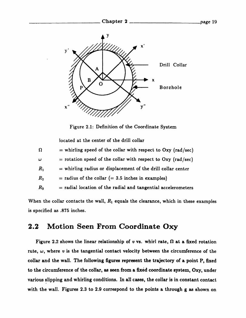
Figure 2.1 is the definition of the coordinate system used to describe the motion
of the drill collar, where :
Oxy = fixed reference frame centered in the borehole
Ox'y' = rotating reference frame with speed n and with its origin
located on the axis of the borehole
Ax"y" = rotating reference frame with speed w and with origin
18
. Chapter 2
y
-------- page 19
Drill Collar
x
Borehole
Figure 2.1: Definition of the Coordinate System
located at the center of the drill collar
n = whirling speed of the collar with respect to Oxy (rad/sec)
w = rotation speed of the collar with respect to Oxy (rad/sec)
R1 = whirling radius or displacement of the drill collar center
R2 = radius of the collar (= 3.5 inches in examples)
Rs = radial location of the radial and tangential accelerometers
When the collar contacts the wall, R1 equals the clearance, which in these examples
is specified as .875 inches.
2.2 Motion Seen From Coordinate Oxy
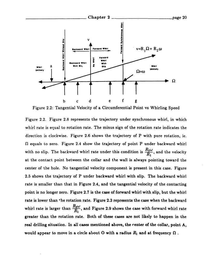
Figure 2.2 shows the linear relationship of t1 VB. whirl rate, 0 at a fixed rotation
r&te, w, where tJ is the tangential contact velocity between the circumference of the
collar and the wall. The following figures represent the trajectory of a point P, fixed
to the circumference of the collar, as seen from a fixed coordinate system, Oxy, under
various slipping and whirling conditions. In all cases, the collar is in constant contact
with the wall. Figures 2.3 to 2.9 correspond to the points a through g as shown on
____________ Chapter 2 -- page 20
.!' V•'JI
••c~••'d Whlrt FOI••,d WN,Ii • ..~
Z• i~• '.clr.••rd Whi,1 •• 0a .. Witll 'Ii~ ZWNrl Iunli'el, •
. v=RtO+ R2(J)
.1'11"""".....,
11
b c d e f g
Figure 2.2: Tangential Velocity of a Circumferential Point VB Whirling Speed
Figure 2.2. Figure 2.8 represents the trajectory under synchronous whirl, in which
whirl rate is equal to rotation rate. The minus sign of the rotation rate indicates the
direction is clockwise. Figure 2.6 shows ttle trajectory of P with pure rotation, ie.
n equals to zero. Figure 2.4 show the trajectory of point P under backward whirl
with no slip. The backward whirl rate under this condition is ~~' and the velocity
at the contact point between the collar and the wall is always pointing toward the
center of the hole. No tangential velocity component is present in this case. Figure
, 2.5 shows the trajectory of P under backward whirl with slip. The backward whirl
rate is smaller than that in Figure 2.4, and the tangential velocity of the contacting
point is no longer zero. Figure 2.7 is the case of forward whirl with slip, but the whirl
rate is lower than the rotation rate. Figure 2.3 represents the case when the backward
whirl rate is larger than ~~' and Figure 2.9 shows the case with forward whirl rate
greater than the rotation rate. Both of these cases are not likely to happen in the
real drilling situation. In all cases mentioned above, the ~enter of the collar, point At
would appear to move in a circle about 0 with a radius R1 and at frequency n .

_____________ Chapter 2 -------- page 21
4 52oINCHES
..2
2
4
-4
.5 ~--L-__--£---.....--.........-_-........-.-J~5 -4
..2
INCHE
o
Figure 2.3: Backward Whirl with Slip, Rotation Speed -2.2 Hz, Whirling Speed 9.9Hz
4 52oINCHES
..2-s I..-....J...__-.L__--..L----..I-----..----
-S -4
5-----..-,---~-----r----,r--,
-4
-2
2
4 -
INCHE
o
Figure 2.4: Backward Whirl, No Slip, Rotation Speed -2.2 Hz, Whirling Speed 8.8 Hz

____________ Chapter 2 --------- page 22
4 52oINCHES
-5 ~-.&...____L..__--...L.__--a.__----t"""'-__
-5 -4
-4
-2
5 ------ -----------.------.~.--.
2
4
INCHE
o
Figure 2.5: Backward Whirl With Forward Slip, Rotation Speed -2.2 Hz, WllirlingSpeed 2.2 Hz
4 S2oINCHES
-2
2
5-------.----.--.-------,..------,r----y---,
4
-4
-2
-5 L..-...J..__--1.__-.L ~_-......-..
-S -4
INCHE
o
Figure 2.6: No Whirl, Pure Rotation, Rotation Speed ·~2.2 Hz, Whirling Speed 0 Hz

4 52oINCHES
-5 L..-..........__---'-__-....__--"__--'_-'
-5 -4
-4
-2
5 ..----.....-------r------.-----r--_-__
2
4
INCHE
o
Figure 2.7: Forward Whirl With Slip, Rotation Speed -2.2 Hz, Whirling Speed -1.1Hz
4 52oINCHES
-2
2
5r-.....,...-----,------,..------r-----.~_
4
-2
-4
-5 '___--'-__.........__......__---1.__---..11.....---1
-S -4
INCHE
o
Figure 2.8: Synchronous Whirl With Slip, Rotation Speed -2.2 Hz, Whirling Speed-2.2 Hz
4 52~5 L--~__---a._--~------""'-'--'
~5 -4 oINCHES
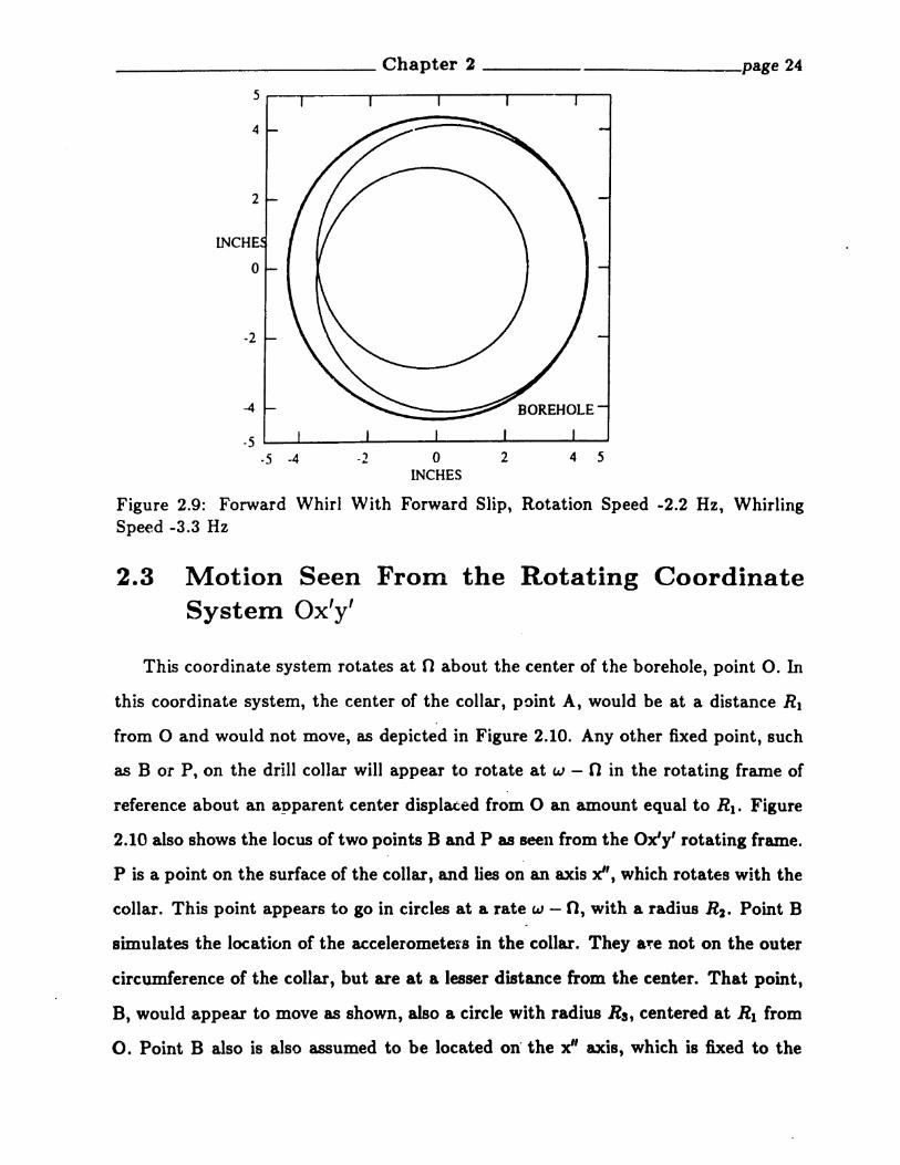
Figure 2.9: Forward Whirl With Forward Slip, Rotation Speed -2.2 Hz, WhirlingSpeed -3.3 Hz
-4
lNCHE
o
2
4
2.3 Motion Seen From the Rotating CoordinateSystem Ox'y'
This coordinate system rotates at n about the center of the borehole, point O. In
this coordinate system, the center of the collar, point A, would be at a distance R1
from 0 and would not move, as depicted in Figure 2.10. Any other fixed point, such
as B or P, on the drill collar will appear to rotate at w - n in the rotating frame of
reference about an apparent center displaced from 0 an amount equal to R1• Figure
2.10 also shows the locus of two points B and P as seell from the Ory' rotating frame.
P is a point on the surface of the collar, and lies on an axis r', which rotates with the
collar. This point appears to go in circles at a rate w - 0, with a radius Rz• Point B
simulates the location of the accelerometers in the collar. They &!e not on the outer
circumference of the collar, but are at a lesser distance from the center. That point,
B, would appear to move as shown, also a circle with radius Ra, centered at R1 from
O. Point B also is also assumed to be located on" the r' axis, which is fixed to the

y" y'
XU
x'
Figure 2.10: Points on the Drill Collar
collar.
2.4 Measurements Taken in a Rotating ReferenceFrame Under Pure Whirl Condition
2.4.1 Bending Moments Bx' and By'
Bending moments are determined by the curvature of the beam as computed with
respect to the neutral axis. In this case, the neutral axis coincides with A, the center
of the collar. The deflection of the collar center as seen in the rotating frame Ox'y' is
designated vo(z) and is assumed to be given by :
(2.1)
vo(z) defines a radial distance from the borehole center(z axis) to the center of the
collar. vo(z) is, therefore, the whirl radius. The function sin(7) accounts for the

radial deflection of the collar center as a function of the distance, %, along the axis from
the bit, as shown in Figure 2.11. Here it has been assumed that the whirl deflected
shape of the collar is half a sine wave between the bit ~d the first stabilizer. Figure
2.10 was drawn assuming one was at the midspan of the collar. At any other z, the
distance to the center of the circle made by B and P would be given by R1 sin(¥) ,and the radii of the circle R2 and Rs would not change. At the bit, fOlr example, the
points Band P as seen in the rotating frame Ox'y' would be circles centered at 0 and
moving at an angular rate of w - n.
The bending moment corresportding to vo(z) is given by the moment curvature
relationship
(2.2)
In the examples drawn from the Shell-NL fields experinlents, the bending moment
B(z) was measured by two perpendicularly mOlJnted strain gages in the Ax"y" system,
which rotates with the collar. But note that B(z) is a two vector components in the
Ax'y' syst~m, with unit vectors i' and j', because the strain gages measure the strain
from the undeflected position, which is the center of the hole.
B(z) = B(z)[sin(w - n)ti' + cos(w - O)tJ·'] =Bz ' + B II , (2.3)
In the example given, the distance, L, from the bit to the center of the stabilizer
was 59~2 feet. The collar outside diameter was 7.0 inches, in an 8.375 inches hole.
A midpoint deflection equal to a clearance of .875 inches would lead to a midpoint
bending moment of 3525 foot-pounds. In the Shell-NL tests, the strain gage location
was typically nine feet above the bit. At the measurement location nine feet above
the bit, the measured bending moment would be reduced to 1600 foot pounds. The
bending moment measurement can be used directly to interpret the whirling motions
of the collar. The magnitude of the bending moment is simply giv-en by
(2.4)

____________ Chapter 2 ------- page 27
Stabilizer
v(z)
Bit
z
1
L
Figure 2.11: Whirl Deflected Shape
A phase angle can be estimated from Bz' and B II, ;
BZI 1 sin(w - n)ttP (t) = tan -1 (-B ) = tan- ( n) = (w - n) t
~' cos w - t(2.5)
tP(t) is simply the phase angle which accumulates at the rotation speed of the collar as
measured in the Ox'y' system. Therefore, from the bending moment measurements,
the magnitude of the whirl can be estimated, and from the phase angle the difference
between,whirl and rotation rate can be determined, but not unique values of wand O.
In contrast, a magnetometer is insensitive to whirl and only sees the rotation of the
collar with respect to the fixed reference frame. Its output is sensitive to the rotation
rate w, but provides no information regarding the whirl rate o.Consider the different whirling conditions described in Figure 2.2 The values of w,
n, and w - n are summarized in the following table for all cases a through g. Note
for this particular table the relative contact velocity with the wall is also presented.
(2.6)
where R1= 0.875 inches, R2=3.5 inches.
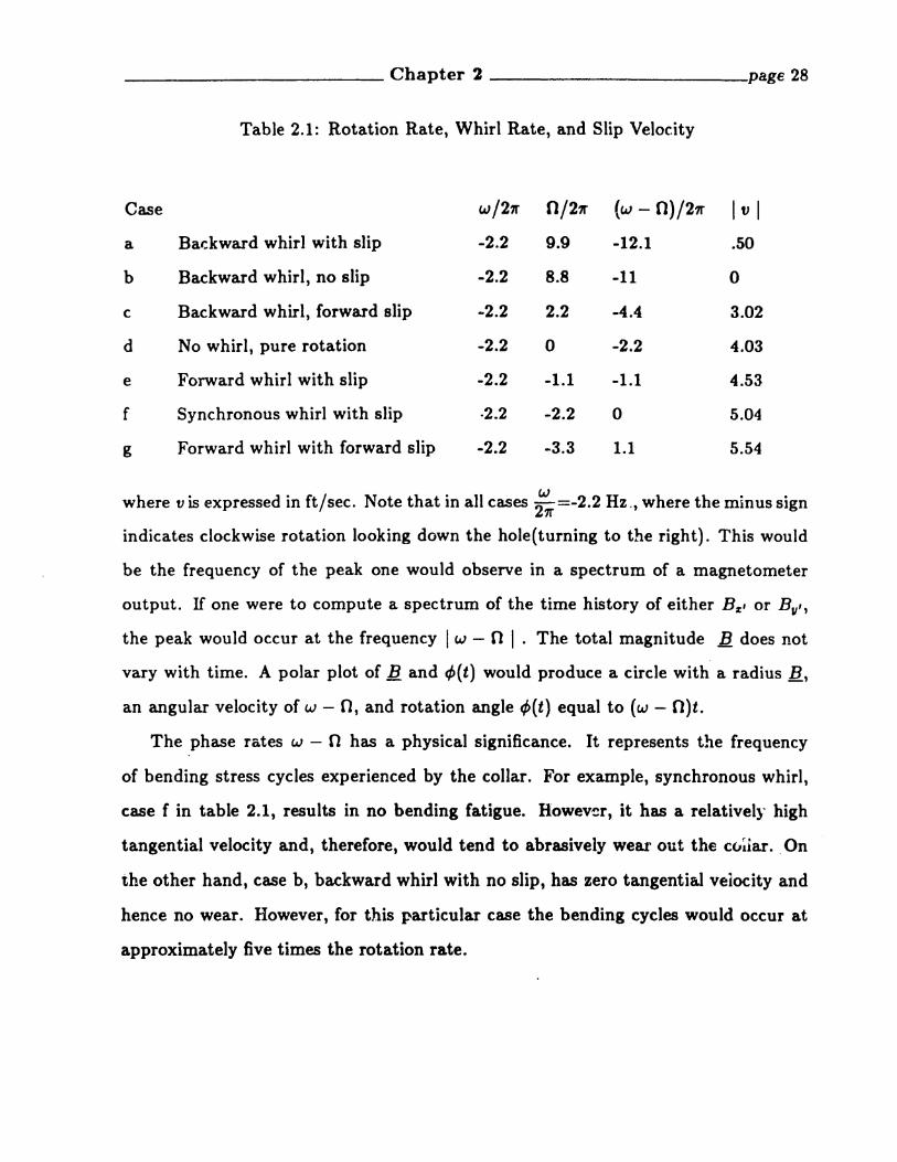
Table 2.1: Rotation Rate, Whirl Rate, and Slip Velocity
Case w/21f n/21f (w - 0)/211" Iv Ia Backward whirl with slip -2.2 9.9 -12.1 .50
b Backward whirl, no slip -2.2 8.8 -11 0
c Backward whirl, forward slip -2.2 2.2 -4.4 3.02
d No whirl, pure rotation -2.2 0 -2.2 4.03
e Forward whirl with slip -2.2 -1.1 -1.1 4.53
f Synchronous whirl with slip -2.2 -2.2 0 5.04
g Forward whirl with forward slip -2.2 -3.3 1.1 5.54
where v is expressed in ftJsec. Note that in all cases ~ =-2.2 Hz" where the minus sign
indicates clockwise rotation looking down the hole(tuming to the right). This would
be the frequency of the peak one would observe in a spectrum of a magnetometer
output. H one were to compute a spectrum of the time history of either B z ' or BII"
the peak would occur at the frequency Iw - n I . The total magnitude B does not
vary with time. A polar plot of Band ¢(t) would produce a circle with a radius B,
an angular velocity of w - 0, and rotation angle t/>(t) equal to (w - O)t.
The phase rates w - n has a physical significance. It represents the frequency
of bending stress cycles experienced by the collar. For example, synchronous whirl,
case f in table 2.1, results in no bending fatigue. However, it has a relativel:r high
tangential velocity and, therefore, would tend to abrasively wear out the culiar.. On
ihe other hand, case b, backward whirl with no slip, has zero tangential veiocity and
hence no wear. However, for this particular case the bending cycles would occur at
approximately five times the rotation rate.

2.4.2 Acceleration Measurements with Radial and Tangentially Mounted Accelerometers Fixed to the Collar ata Radius Rs
Accelerometers measure absolute acceleration regardless of reference frame. There
fore, a radially oriented accelerometer mounted at a radius Rs from the collar center
would respond to the radial acceleration, Raw2 , with respect to the center of the collar,
as well as the component of the whirl acceleration of the collar center in the direction
of the radially mounted accelerometer. This component is given by R102 cos(w - O)t.
A tangential accelerometer would not feel any centripetal acceleration du(, to the col
lar rotation, but would respond to the tangentially oriented component of the whirl
acceleration of the collar center. Therefore, we may write
ar - R1n 2 cos(w - n)t + Rsw2
at R1n2 sinew - O)t
(2.7a)
(2.7b)
where ar is the radial acceleration, and ac is the tangential acceleration. If the ac
celerometers are of the piezoelectric type, they can not measure constant acceleration
components. Thus, the Rsw2 term of the radial acceleration would not be measured,
and the acceleration magnitude as measured would be
and the phase angle
1
~ = (a~ + a:)2 = R10 2 (2.8)
<p(t) = tan-I (tit) = (w - O)t (2.9)a,
In the case of synchronous whirl, w - n = 0 and both a,(t) and a,(t) would not vary
with time. In that case t the output of the aecelerometers would be zero, due to the
low frequency limitations of piezoelectric accelerometers. In reality, the drill collar
may exhibit dynamic behavior other than pure whirling motion as described thus
far. For example, torsional vibration will lead to non-zero tangential acceleration. In
the previous discussion of acceleration and bending measurements, the phaae angle

____________ Chapter 2 _ page 30
4>(t)=(w-O)t and ~ =0. Torsional vibration would introduce a tangential acceleration
component Rs¢. Similarly, transient impacts with the wall would cause tangential and
radial accelerations which are not as simple as cases of pure whirl. Bendin~ data are
in practice very difficult to interpret when non-whirling caused vibration occurs. An
example is discussed in the next section.
2.5 Measurements Taken on a Rotating Frame WithSimultaneous Whirling and Bending Vibration
Rotation and mass eccentricity cause a shaft to whirl. The ampU: ·,ne o~ .~'
whirling depends on the eccentricity, and on the closeness of the Jotatlon SPC{ anlt
the bending natural frequencies of the shaft. The whirling amplitude grows larger as
the rotation speed approaches one of the natural frequencies. But as the collar whirls,
bending"vibrations can also be excited, for example, by lateral or axial dynamic forces.
Depending on the reference frame, these motions may seem simple or very complex.
An observer in the fixed coordinate system describes synchronous whirl as a cir
cular motion of the shaft. But to an observer staying in the center of the coordinate
system OX'Y', rotating at 0, whirl is just a constant deflection. Assume that in addi
tion to this constant deflection, the rota:ting observer also witnesses a simple circular
motion of the center of the shaft about the constant deflection center. The equations
describing the motion of the sha.ft center as seen by this person are:
x'{t) - Rz ' coswnt
1I'{t) - R,. sin wnt
(2.10a)
(2.10b)
where Rz, and R" are the amplitude of the bending vibration and Wn is the bending
vibration frequency relative to the rotating coordinate system. The trajectory seen
from a non-rotating reference frame is given by:
x(t) - R1 cos(wt) + Rz' cos(wnt) cos(nt) - R,. sin(wnt) sin(nt)
y(t) - R1 sin(wt) + R~J cos(wnt) sin(nt) + R" sin(wnt) cos(Ot)
(2.11a)
(2.11b)
_____________ Chapter 2 page 31
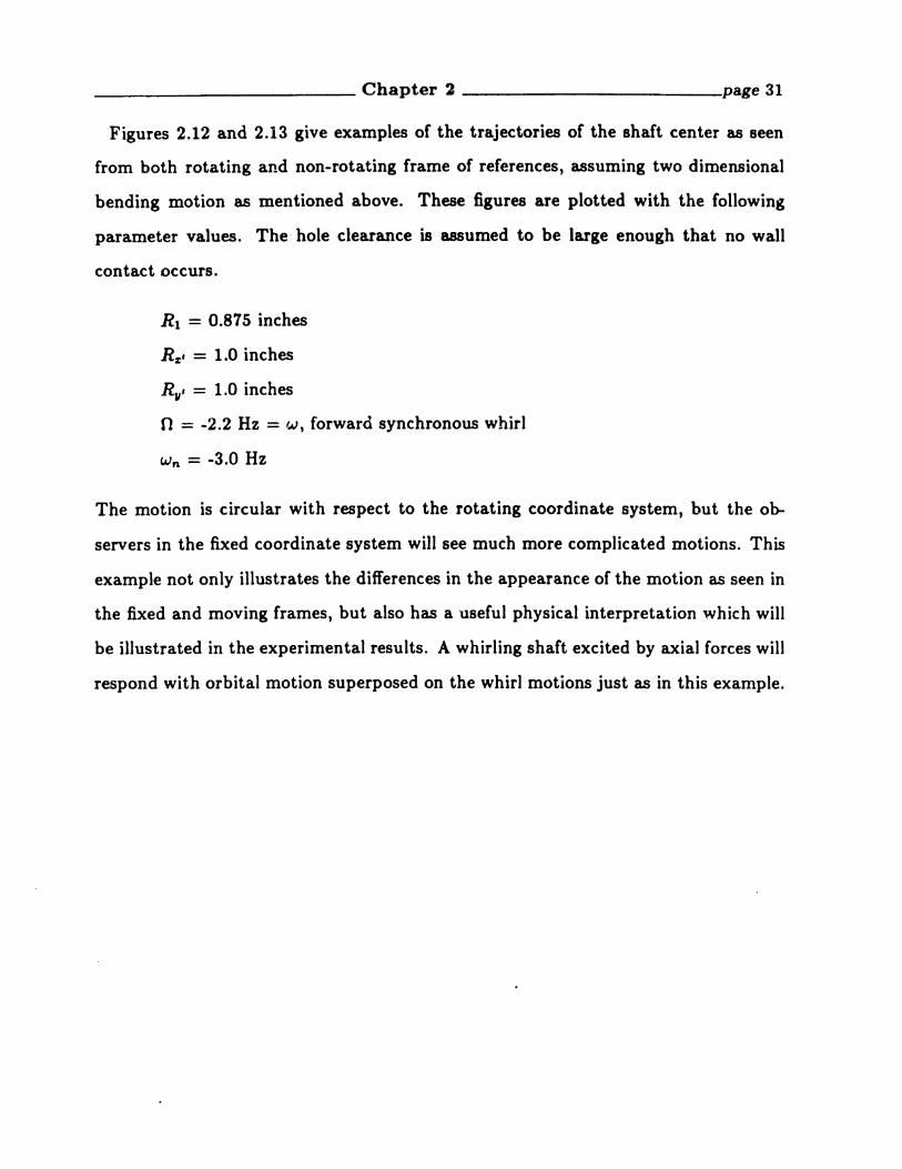
Figures 2.12 and 2.13 give examples of the trajectories of the shaft center as seen
from both rotating and non-rotating frame of references, assuming two dimensional
bending motion as mentioned above. These figures are plotted with the following
parameter values. The hole clearance is 88Sumed to be large enough that no wall
contact occurs.
R1 = 0.875 inches
Rz' = 1.0 inches
RJlI = 1.0 inches
n = -2.2 Hz = w, forward synchronous whirl
W n = -3.0 Hz
The motion is circular with respect to the rotating coordinate system, but the ob
servers in the fixed coordinate system will see much more complicated motions. This
example not only illustrates the differences in the appearance of the motion as seen in
the fixed and moving frames, but also has a useful physical interpretation which will
be illustrated in the experimental results. A whirling shaft excited by axial forces will
respond with orbital motion superposed on the whirl motions just as in this example.

____________ Chapter 2 -------- page 32
4 52oINCHES
-2
.5 "__......Ao.o.__-Ao__-.......I.....-__ooI.-__.........-J
-5 -4
5 ROTAnON SPEED -2.2 Hz, VIBRATING FREQ. ·3 Hz
-4
-2
2
4
INCHE
o
Figure 2.12: Motion Seen From the Fixed Coordinate System
5 ROTAnON SPEED -2.2 Hz, VIBRATING FREQ. -3 Hz
4 S2oINCHES
-2
2
4
-2
-4
-s ~-....__--..._-_a...-__..&.-__-'--J
-5 -4
INCHE
o
Figure 2.13: Motion Seen from the Rotating Coordinate System

Chapter 3
The Bending Natural Frequenciesof Rotating Drill Collars
The bending vibration of the BHA is less well understood than torsional or axial
vibration. Relatively, few papers have been devoted to the study of this phenomenon.
The lack of research is partly due to the fact that bending vibrations downhole seldom
propagate to the top, and to the lack of downhole measurements. Therefore, we begin
with the discussion of the bendirlg vibration of the drill collars.
3.1 Basic Configurations of the BHA
The arrangement of the stabilizers in the BHA affects the direction of the borehole.
Depending on the location of the stabilizers, BHAs can be categorized as building,
holding, or dropping assemblies. Figure 3.1 shows five configurations of the BHA.
Accordi~g to drilling practice, BHA no.1 is rated as a dropping assembly; BHA no.2
is found to be a very strong dropping assembly; BRA 00.3 is rated as a very strong
building assembly; BRA no.4 is found to act as a good holding assembly; BHA no.5 can
be used as a weak building or a weak dropping assembly, dependiIlg on hole geometry
and the interaction between the stabilizer and the- formation. The placement of the
stabilizers also affects the bending natural frequencies of the DBA. The simpliest
approach, and the one taken here, is to model the effect of the bit and stabilizers
with equivalent boundary conditions. Thus, a BRA is modelled as an axisymmetric,
33

bit
0
060' g 30' g2
Og 90· g3
to' 30'
4 Og g g
Og 30' g5
Figure 3.1: Several Configurations of the BHA
rotating, ~nultispan beam. The spans are determined by the placement of the bit
and stabilizers. With this approach, BHA number 2 in Figure 3.1 might be modelled
as a tv/o span beam that is hinged at the bit, restrained in displacement at the
first .stabilizer. and given a displacement and moment spring restraint at the second
stabilizer. Such a model, then, approximates the effect of the BRA above the second
stabilizer by a simple spring. Depending on the value of the spring constant, this
restraint can be varied from a simple hinged to a built-in (fixed) condition. This
simple approach will provide estimates of the natU!al frequencies and mode shapes
for bending vibration between the bit and the second stabilizer only.

(3.1)
3.2 Theoretical Background
Figure 3.2 shows a section of BHA near the bit. The coordinate systems for the
drill collars are shown in Figure 3.3. The homogeneous governing equation for bending
vibration for a rotating beam in the z direction is [42]:
ApCMx = -EI::~ + Q~~ - (CE + C/ )% + CIWY
82,; ax-ApghcostP[(l- z) az2 - az J + ApCMaw2 coswt
the !I direction is:
lJ4 y aSyApCMy = -EIaz. - Qazs - (CE + C/)y - C1wx
-Apghcos tP[(1 - z) ::~ - :~) + ApCMbw2 sin wt - Apgh sin tP (3.2)
if complex notation a' = x + iy and e' = a + ib are used, and dividing through by
ApCM , then
(3.3)
. The definition of each symbol is
A = cross sectional area of collar
p, Pm = density of steel and mud
GE ,OI = external and internal damping
E I = flexural rigidity
9 = gravity constant
tP = slant angle of drill collar
OM = mass coefficient of collar = l+(added mass of mud per unit length +
· mud maos per unit length trapped inside the collar) / collar mass
per unit length

____________ Chapter 3 --------- page 36
Slant
Mud
Collarz
1..
Stabilizer
Lb.OD2.1D2
Stabiliz.er
La,ODI.IOl
Bit
Figure 3.2: BHA Near the Bit
h = I_Pmp
1 = weight on bit/Apghcost/>
Q = torque
w = rotation speed of the ·drill collar
e' = mass eccentricity of the collar
The undamped natural frequencies and mode shapes for the non-rotating drill collars
may be sought by first setting the damping and rotating speed, w, to zero, and
assuming static side force does not affect the natural frequency. The equations of
motion can be expressed in a dimensionless form as follows. Let La = length of drill
collar form the bit to the first stabilizer
w -
EIw~ - ApCML:
zLa
(3.4a)
(3.4b)

Cros~ Section of a Drill Collar
y+b)' --+-.......-
x x+a
OXY : fixed reference frame
x·
G gravity center
C geometric center
(a.b) : eccentricity of the collar
(i) rotation speed of the collar
OX'Y' : rotating reference frame
Figure 3.3: Coordinate System
T - wot (3.4c)s'
(3.4d)s -La
11I
(3.4e)-La
then
8 28 8 48 .QLG aSs gh cos cP 8 28 as
a.,2 + aw4 + I EI aws + LGCMW~ [(11 - w) aw2- awl = 0 (3.5)
By separating the time and spatial variables and using the central difference method
to replace the spatial derivatives, the differential equation can be transformed into a
system of algebraic equations. For details see Appendix A.
where
[D][s] = 0
[D] is a n x n finite difference matrix
(3.6)
w=l+Lb/La
w=l
w=o
j=N Stabilizer
j=M Stabilizer
j=2
j= 1
j=O Bi t
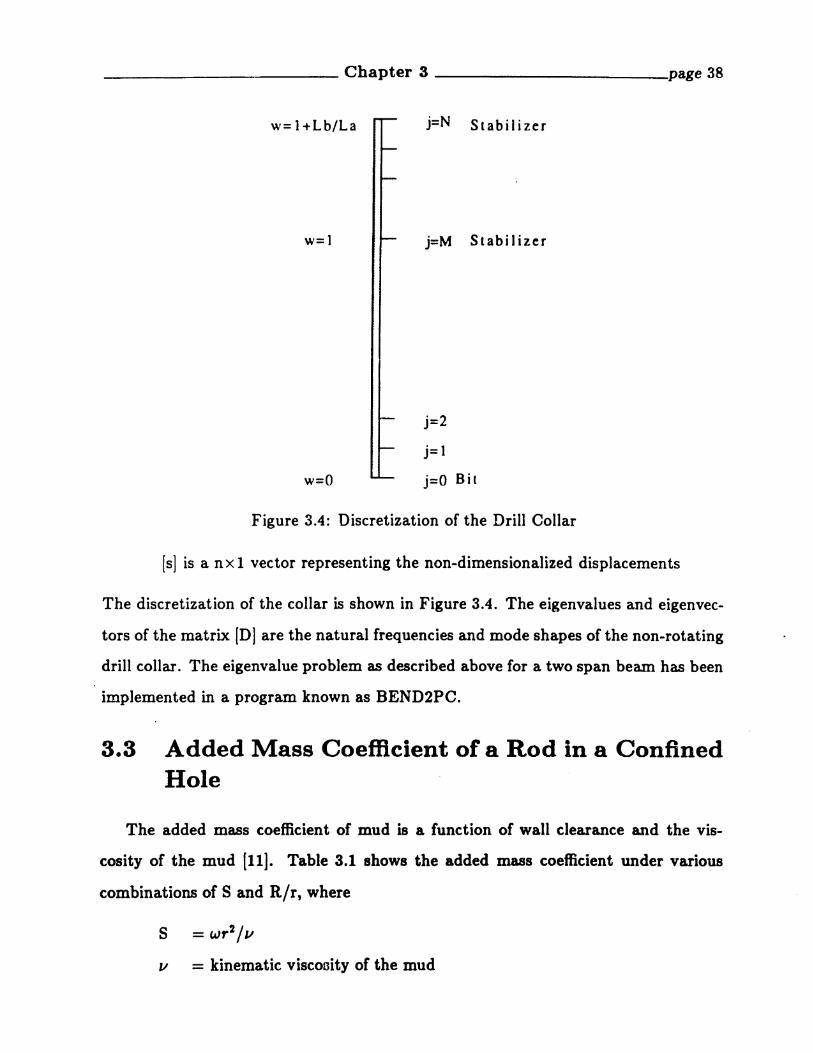
Figure 3.4: Discretization of the Drill Collar
(s] is a nx 1 vector representing the non-dimensionalized displacements
The discretization of the collar is shown in Figure 3.4. The eigenvalues and eigenvec
tors of the matrix [D] are the natural frequencies and mode shapes of the non-rotating
drill collar. The eigenvalue problem as described above for a two span beam has been
implemented in a program known as BEND2PC.
3.3 Added Mass Coefficient of a Rod in a ConfinedHole
The added mass coefficient of mud is a function of wall clearance and the vis
cosity of the mud [11]. Table 3.1 shows the added mass coefficient under various
combinations of S and Rlr, where
S = wr2/v
v = kinematic visconity of the mud

Table 3.1: Added Mass Coefficient of a Vibrating Rod in a Confined hole
~ 50< 1000 2000 3000 SOOO
1.2 6.88 6.83 6.54 6.38 6.21
1.3 4.86 4.63 4.43 4.34 4.24
1.4 3.75 3.57 3.43 3.37 3.311.5 3.11 2.97 2.86 2.81 2.76
1.6 2.70 2.51 2.49 2.45 2.42
1.7 2.41 2.31 2.23 2.20 2.111.8 2.19 2.11 2.05 2.02 1.991.9 2.04 1.96 1.90 1.88 1.852.0 1.92 1.84 1.19 1.71 1.14
2.2 1.74 1.67 1.63 1.61 1 59
2.4 1.62 1.56 1.52 1.50 1.48
2.6 1.53 1.47 1.44 1.42 1.41
2.8 1.46 1.41 1.38 1.36 1.353.0 1.42 1.36 1.33 1.31 1.30
3.5 1.33 1.28 1.25 1.24 1.23
4.0 1.27 1.23 1.21 1.19 1.18
5.0 1.22 1.18 1.15 1.13 1.12
6.0 1.19 1.15 1.12 1.11 1.108.0 1.16 1.12 1.10 1.08 1.07
10.0 1.14 1.11 1.08 1.07 1.06
R = radius of the hole
r = outer radius of the collar
w = vibration frequency in radians pe~ second
The coefficients in Table 3.1 can also be obtained through following formula,
[0:~(1 + "'12) - 8"'1] sinh(p - 0:) + 20:(2 - "'1 + "'12
) C08h(/1 - "'1) - 2"'12[0:/1 - 20:~0", = Re( )
0:2(1 - "'12) sinh(/1 - 0:) - 20:"'1(1 + "'1) C08h(P - 0:) + 2"'12V;;P + 20: ;
(3.7)

70
60!I >,
,,~.§ u..en ! .su 50 =en i§0Q..- 40s::CJu
~ 30en0Uen 20>
10
0
8.3 8.7 9.1 9.5 9.9 10.3 10.7 11.1
Mud weight, ppg
Figure 3.5: Viscosity of Drilling Muds
where Re indicates the real part of a complex quantity, ex = kr, P = kR, "y = ~,
and k = ~. Equation 3.7 is valid if both a and P are greater than 10. Figure 3.5
shows the viscosity for various drilling muds. To convert viscosity from centipoises to
kinematic viscosity in /t 2 / sec, the following formula are needed.
poises= centipoises/lOO
p = mass density of the mud (slug/ItS)
v = kinematic viscosity (ft 2 / Bee) = poises/497p
3.4 Effects of WOB and TOB on the Bending Vibration
A numerical example is given to show the effects of the WOB and TOB on
the bending natural frequencies. The numbers used as the inputs to the program
____________ Chapter 3 --------- page 41
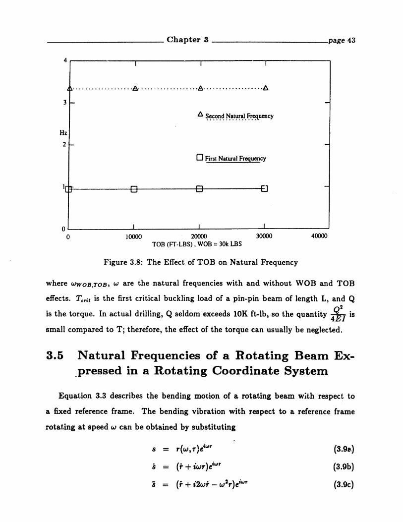
BEND2PC are shown in the Table 3.2. The first two modes are shown in Figure
3.6. Figure 3.7 shows the effect of the WOB and Figure 3.8 shows the effect of the
TOB on the natural frequency of these modes. During Chilling operations, the WOB
may reach SOK Ibs, but the TOB seldom exceeds 10,000 ft-lbs. So, from Figures 3.7
and 3.8,. we can conclude that the effect of TOB on bending natural frequencies can
usually be neglected. This assumption is made in chapter 4.
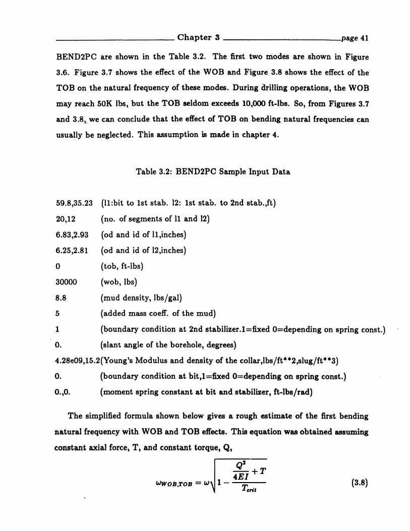
Table 3.2: BEND2PC Sample Input Data
59.8,35.23 (ll:bit to 1st stab. 12: 1st stab. to 2nd stab.,ft)
20,12 (no. of segments of II and 12)
6.83,2.93 (od and id of Il,inches)
6.25,2.81 (od and id of 12,inches)
o (tab, ft-Ibs)
30000 (wob, lbs)
8.8 (mud density, lbs/gal)
5 (added mass coeff. of the mud)
1 (boundary condition at 2nd stabilizer.l=fixed O=depending on spring canst.)
o. (slant angle of the borehole, degrees)
4.28e09,15.2(Young's Modulus and density of the collar,lbs/ft·*2,slug/ft**3)
o. (boundary condition at bit,l=fixed O=depending on spring canst.)
0.,0. (moment spring constant at bit and stabilizer, ft-Ibs/rad)
The simplified fonnula shown below gives a rough estimate of the first bending
natural frequency with WOB and TOB effects. This equation was obtained assuming
constant axial force, T, and constant torque, Q,
Q2-4El+ T
WWOB,TOB = W 1 - (3.8)Tent

-----------Chapter 3 page 42
First Mode, 0.95 Hz Second Mode, 3.33 Hz
Stabilizer
Stabilizer
Bit
Figure 3.6: First Two Bending Modes
4------~-----~-----._----____,
···················A ~ .~ ~
3
Hz
2
o First NalW"al Frequency
oL-----.L------..L-.-----..I..-----40000~o 10000 20000 30000
WOB(LBS)
Figure 3.7: The Effect of WOB on Natural Frequency
____________ Chapter 3 ------ page 43
4 ,..----...----.-------.....--------..,.-------.......,
" ·A· ·A···················l!J.
3
Hz
2
o Firsl Natural Frequency
4()(XX)]ססoo 2()(xx) ooסס3
TOB (FT·LBS), WOB = 30k LBS
OL....-------~------........L-------~------o
Figure 3.8: The Effect of TOB on Natural Frequency
where WWOB,TOB, ware the natural frequencies with and without WOB and TOB
effects. Terif is the first critical buckling load of a pin-pin beam of length L, and Q
is the torque. In actual drilling, Q seldom exceeds 10K ft-lb, so the quantity 4~I is
small compared to T; therefore, the effect of the torque can usually be neglected.
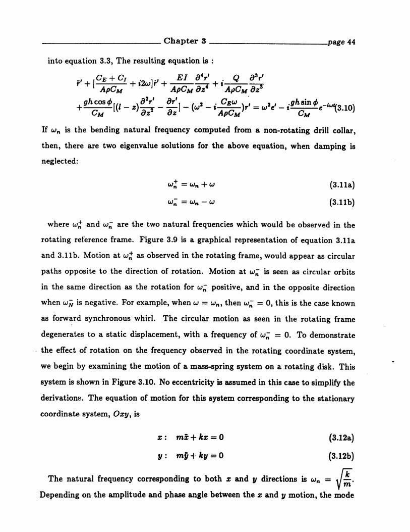
3.5 Natural Frequencies of a R,otating Beam Ex.pressed in a Rotating Coordinate System
Equation 3.3 describes the bending motion of a rotating beam with respect to
a fixed reference frame. The bending vibration with respect to a reference frame
~otating at speed w can be obtained by substituting
s - r(w ,,\eiwf' (3.98.), J
8 - (r + iwr)e'c,,,· (3.9b)
:9 - (f + i2wr - w2r)eiwr (3.9c)
_____________ Chapter 3 -------- page 44
into equation 3.3, The resulting equation is :
, rOE + 0 1 • l.' EI a4r' . Q a1J
r'r + ApCM + 12w r + ApCM ai- + I AIlC
Maz3
ghcosq,[(l )02r' or'] (2 · CEW ) " 2' .ghsint/J -illJ"3 10~+ -Z~---W-I r=we-I e \. JeM 8z 8z ApCM OM
If Wn is the bending natural frequency computed from a non-rotating drill collar,
then, there are two eigenvalue solutions for the above equation, when damping is
neglected:
w~ =Wn+W
w~ = Wn - W
(3.11a)
(3.11b)
where w; and w; are the two natural frequencies which would be observed in the
rotating reference frame. Figure 3.9 is a graphical representation of equation 3.11a
and 3.11b. Motion at w~ as observed in the rotating frame, would appear as circular
paths opposite to the direction of rotation. Motion at w; is seen as circular orbits
in the same direction as the rotation for w; positive, and in the opposite direction
when w'N is negative. For example, when w = Wn , then w; = 0, this is the case known
as forward synchronous whirl. The circular motion as seen in the rotating frame
degenerates to a static displacement, with a frequency of w; = o. To demonstrate
. the effect of rotation on the frequency observed in the rotating coordinate system,
we beg.in by examining the motion of a mass-spring system on a rotating disk. This
system is shown in Figure 3.10. No eccentricity is assumed in this case to simplify the
derivations. The equation of motion for this system corresponding to the stationary
coordinate system, Ozy, is
x: m!+ lex = 0
11: my -f. ky = 0
(3.12a)
(3.12b)
The natural frequency corresponding to both % and 71 directions is Wn = ~.Depending on the amplitude and phase angle between the x and JJ motion, the mode

______________ Chapter S page 45
co
a
ro - 00nm+oon
ro-n
natural frequency
Figure 3.9: Frequencies Observed in a Rotating Coordinate
Rotating Table
ro Rotating frequency
ron. Natural Frequency
Figure 3.10: Mass-Spring System on a Rotating Table

_____________ Chapter 3 -------- page 46
shape can be circular, or elliptical, and may rotate in clockwise or counterclockwist.;
direction. The equation of motion for this system corresponding to the rotating
coordinate system, ary', is
x': m(:? + 2wy' - w2z') + lex' =0
yl: m(y' - 2wZ. - W211') + ky' =0
(3.13a)
(3.13b)
where x' and y' are the coordinates fixed on the disk, m and k are the mass and
stiffness respectively. The above equation can be written in operator form 88,
Z: LIZ' + L 2y' = 0 (3.14a)
y: Lsx' + L4.Y' = 0 (3.14b)
where
L1 - D 2_ w2 + w 2 (3.15a)n
L 2 - 2wD (3.ISh)
L s - -2wD (3.1Sc)
L4 - D2 _ w2 +w2 (3.15d)n
Dd
(3.15e)-dt
The solutions to this system of differential equation are the roots of
(3.16)
By solving this equation, the homogeneous solutions for :1:' and y' can be written as
follows:
x' = Ale-iCwn+W)f + Ate'Cw,,-w)' + Aaei(w,,+W)f + A..e-i(W,,-W)f
1/' = B1e-i(Wn+W)f + B2ei (w,,-w)' + Baei(w,,:+w)' + B4e-i (w,,-w)'
(3.17a)
(3.17b)
The clockwise direction indicates the the direction of decreasing angle, and coun
terclockwise direction indicates the direction of increasing angle. Therefore, if the

_____________ Chapter 3 page 47
direction of rotation of the drill collar is clockwise, indicating that the rotation rate
is -w, then, the coefficients As, A4 , Bs, and B. will vanish. On the other hand, if
the direction of rotation is counterclockwise, the coefficients AI, A2 , B1 , and B2 will
vanish. The ratio of ~: indicates the mode shape of their associated eigenvalues.
For example, the ratio of*shows the mode shape of eigenvalue -i(w + wn ). The
ratio of*can be obtained by substituting equation 3.17a into equation 3.13b, and
setting A2 , As, A., B 2 , Bs, and B. equal to zero. Following this procedure, we can
find that the mode shape for eigenvalues -i(wn ± w) is -i, and the mode shape for
eigenvalues i(wn ± w) is i, if Wn ± w remains positive. This implies that rand y' are
equal in.magnitude, but 90 degrees out of phase with each other, which would be seen
as circular motion in the rotating frame. The direction of rotation depends on the
sign of the eigenvalue. A positive eigenvalue indicates a counterclockwise rotation,
whereas, a negative eigenvalue indicates a clockwise rotation. IT we assume that there
is an sinusoidal input force in the x' direction designated as PetwLt , the particular
solution can be obtained by assuming the solution in the form
(3.18a)
(3.18b)
Substituting this into the equation of motion and solving for Al and B I , we find
that
Alw2 -wl-w2
- e
B Ii2wWL
- e
(3.19a)
(3.19b)
where e is
(3.20)
If we demand that IAII = IBII, then, it implies that WL = W ± Wn • Physically, it
means that if the excitation frequency equals to one of the natural frequencies, then,
____________ Chapter 3 ------- page 48
the motion of the mass is a circle with respect to an observer who stays in the center
of the disk. Following a similar argument, it can be shown that if the excitation
frequency frequency is not at a natural frequency, then the ratio of ~: can not be
1.0. The resulting motion will be elliptical in shape.
3.6 Several Interpretations of the Results
The bending natural frequencies with respect to a fixed coordinate system deter
mine the rotation speeds at which large amplitude forward synchronous whirl occurs.
The closer the rotation speed comes to the natural frequenci~,sas computed in a fixed
reference frame, the larger the whirling amplitude. Synchronous whirl at this rotation
speed may cause excessive wear on one side of the drill collar, or may result in back
ward whirl if the wall friction is sufficiently high. One the other hand, the natural
frequencies with respect to a rotating coordinate system determine the frequencies of
external excitations that will cause large bending vibration. Therefore, the excitations
needed to drive the collar into large bending motion vary linearly with the rotation
speed of the drill collar. Examples of bending Vibration due to external excitation
are shown in the experimental results in chapter six, which contains the predictions
given above. Examples of forward and ~ackward whirl are given in chapter seven.
Chapter 4
Axial Excitation of BendingVibration
In actual drilling, dynamic axial forces are produced because of the interaction
between the bit and the formations.. These axial forces can induce bending ,'ibra
tion. There are two principal types of bending vibration resulting from axial forces.
In this thesis, they are termed linear coupling and parametric coupling. These cou
pling mechanisms between axial forces in the drill string and bending vibrations are
described in the following sections.
4.1 Linear Coupling of Axial Force and Bending
Line~r coupling between the axial forces on the bit and bending vibration occurs
frequently in real drilling assemblies, often superposed on other bending vibration
phenomena. The source of linear coupling is initial curvature of the BHA, such as
is depicted in Figure 4.1. Linear coupling is easy to visualize by taking a thin ruler
or a piece of paper, giving it a slight curve, and then pressing axially on the ends.
The object responds by additional bending in the plane of the initial curvature. The
frequency of the bending and axial vibrations is the same. The coupling is made
possible by the initial curvature. Linear coupling will not occur on a perfectly straight
beam excited by an axial load which is less than the critical buckling load. However,
if there is any initial curvature, an axial load will cause a lateral deflection. For
49

(4.1)
____________ Chapter 4 --------- page 50
t Axial Force
....--- Drill Collar·
Collar with Initial Curvature
tAxial Force
Figure 4.1: A Section of a Bent Collar
small amounts of curvature, the greater the initial curvature, the greater the lateral
deflection. Of course, curvature is very common in bottom hole assemblies due to the
combined effects of gravity and axial force in inclined holes. Whirling also results in
curvature of the BHA and, therefore, also leads to coupling. Dynamic variations in
the weight on bit then cause bending vibration to occur about the mean statically
deflected shape.
4.2 Linearly Coupled Equations of Motion
The equations of motion describing coupled axial and bending vibration are given
below for the non-rotating beam. Rotation will be introduced later. In the axial
direction:
a2u a au a'y aSxAp-2 = -8EA(-a - It"X + lCe1l) - El(lCep -/til ~ s)at z z Z uZ
in the z direction, where z is measured from the initially curved position:
a4z aszApOMX = -EIaz4 + Q azs - (OE + 0 1 )% (4.2)
a2x ax auApghcostj>[(l- z) az2 - az1+ EAltf(az -ltf X + 1'&11)

_____________ Chapter 4 page 51
in the II direction, where !I is measured from the initially curved position:
a4y aSyApCMY = -EIOZ4 - Qozs - (CE + CI)iJ (4.3)
a2y By auApghcos4>[(l- z) OZ2 - ozl + EAlez(oz - Ie"X + lezy)
where
· · · 1 tId· t Q d2ZoK,z = Inltla curva ure a ong x JTee: Ion == tizr
Ie" = initial curvature along y direction = dd2Y
;f.%
where xo(z) and yo(z) are the initial f:urved shapes
This set of equations indicates that the coupling mechanism of axial and bending
is the curvature of the drill collars. Without the curvature, the axial and bending
vibration will respond independently, according to linear beam theory. A similar
result may be found in [41]. The above equation was solved by central finite difference
scheme. Figure 4.2 depicts the BHA model that was used for the calculations. It is
a standard pendulum BHA with two stabilizers. The boundary conditions at the bit
were specified as lateral displacements and bending moments equal zero. At the first
stabilizer, the lateral deflection was zero. The boundary conditions at the second
stabilizer were specified as lateral displacements and slopes equal zero. Due to the
curvature induced by axial load, gravity, or eccentricity of the collars, the bending
natural frequencies may shift slightly with respect to an unbent configuration. Figure
4.3 shows the effect of the curvature on the first bending natural frequency of the BRA
shown in Figure 4.2. In this ex~ple, the initial deflection shape tJo(z) was assumed
to be in the first mode shape. The maximum value of Va occurs at the midpoint of
the longer drill collar section.. A measure of the ini~ial curvature is given by the ratio
~, where LA is the unsupported span length. This ratio is plotted versus the
first mode bending natural frequency in Figure 4.3 The natural frequency, due to the
coupiing effect, decreases with increasing curvature. For a. borehole with a radial wall
clearance of 4 inches and a span of 59 feet, this ratIo is approximately 0.005 resulting

stabilizer 2 T35.2'
stabilizer 1
59.2'
bi t
z
Figure 4.2: Drill String Model for the Linear Coupled Example
0.9 o First Natural Frequency
Hz
0.8
0.0150.010.005Curvature oi me Orin CoHar
0.7 "'---------..........---------........---------o
Figure 4.3: The Effect of the Curvature on the Natural Frequencies
_____________ Chapter 4 ------- page 53
in a decrease of less than 5 percent in natural frequency. To further understanding
of linear coupling, one might consider the term ~~ in both x and y equations of
motion. Physically, this term represents the axial strain' along the drill string:. If the
axial strain were to vary harmonically in time due to dynamic variations in WOD, it
would assume the form dd~Z)eiwt • This term may be thought of as the input forcing
function, and because the equations are linear, the solution for both x and y will be
harmonic at the same frequency.
In actual drilling practice, the borehole diameters are often only one to two inches
larger than the drill collars. So, the curvature of the drill collars is limited by the
diameter of the hole. In a pendulum BRA, the first stabilizer is placed about 60 ft
above the bit; therefore, the curvature of the collar is very small, and the effect of
the curvature on the drill collar bending natural frequency can be neglected, as men
tioned above. Although the changes in bending natural frequency can be neglected,
the curvature does induce bending vibration which may be problem. An example
demonstrating this phenomenon will be shown in chapter 6.
4.3 The Effect of Rotation on the Linear CouplingPhenomena
The equation shown above is described in terms of a stationary coordinate system.
But, as" was mentioned in chapter 3, the natural frequency observed in a rotating co
ordinate system will vary with rotation rate. This also implies that the frequency of
axial excitation needed to drive the collar int~ large resonant bending vibrations will
change, according to the rotation speed of the drill collars. For example, if the drill
string is stationary, the axial frequency needed to drive the collar at a bending reso
nance is equal to Wn , the natural frequency of the drill collar, provided the curvature
is small. But, as the drill string starts to rotate at w, the axial frequency needed to
drive the collar into bending resonance will change from Wn to IWn ± wI. This concept
is not intuitively obvious, but it is essential to understanding drill collar vibration.

____________ Chapter 4 -------- page 54
The equations of motion expressed as seen in the rotating reference frame are 88
follows, in the axial direction :
(4.4)
in the z direction:
84% B3z
- --EI8z" + Q 8zs - (OE + 0 1 )% (4.5)
a2z ox auApghcost/>[(l- z) 8z" - 8z J+ EAtc,(8z -IC.,X + 1C1:1I)
in the y direction:
84y aSy- -EI8z" - Q8zs - (OE + OI)fJ (4.6)
&2 y oy auApghcost/>[(l - z) 8z2 - a) + EAIC%(8z - IC.,X + 1C%1I)
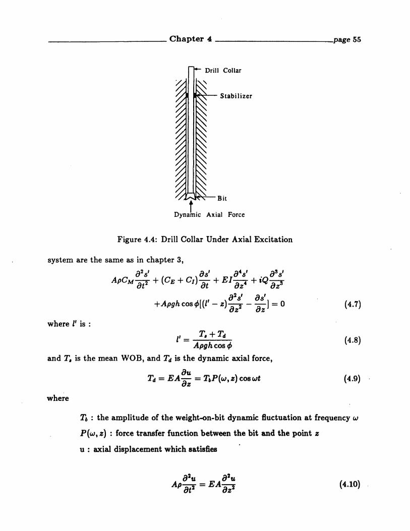
4.4 Bending Vibration of the BHA With Parametric Excitation Without Wall Contact
The bending vibration can be excited parametrically by the dynamic axial exci
tations. It occurs usually when the shaft is straight, and with strong dynamic axial
forces coming from the bit rock interactions as shown in Figure 4.4. This phenomenon
is most likely to occur in the section between bit and the first stabilizer in a pendulum
assembly or the section above the uppermost stabilizer t if the BHA is vertical. The
most distinguishing feature of p&:rametrically excited vibration is that the bending
response frequenclF is one half the axial excitation frequency. This phenomenon is
demonstrated in the laboratory experiments descri~ed in chapter 6.
4.5 Equation of Motion
The following equation includes the effect of parametric axial excitation on bending
vibration for a non-rotating beam. The definition of the symbols and the coordinate
____________ Chapter 4 ---- page 55
~~ Stabilizer
Bit
DynaliC Axial Force
Figure 4.4: Drill Collar Under Axial Excitation
system are the same as in chapter 3,
a2s' as' 8 48' ass'ApCMat! + (CE + Cr) 8t + EI 8z. + iQ 8zs
82s' as'+Apghcos4>[(I' - z) 8z2 - 8z l = 0
where l' is :
I' = T. + TdApghcostj>
and T, is the mean WOB, and Ttl is the dynamic axial force,
auTd = EA 8z = T6P(w, z) cos wt
where
(4.7)
(4.8)
(4.9) .
Tb : the amplitude of the weight-on-bit dynamic fluctuation at frequency w
P(w, z) : force transfer function between the bit and the point z
u : axial displacement which satisfies
(4.10) .

____________ Chapter 4 --------- page 56
IT the length of the section considered is short compared to the wave length of the
axial vibration, P(w, z) can be assumed to be unity. This is a realistic approximation
near the bit in actual drilling conditions. Typical bofttom hole 88semblies consist
of two or three drill collars below the first stabilizer. This section of drill collars is
susceptible to parametric bending vibrations, due to large dynamic variations in the
weight on bit. Usually, each drill collar is 30 feet long, 80, the total length below the
first stabilizer is less than 100 feet long. The axial wave length in steel drill collar is
about 16,000 feet at a frequency of 1 Hz. So, we can neglect the dynamic axial stress
variations along this section of the drill collar.
The equation above can be nondimensionalized using w = i, 1 = ~ and .,. = w~t.
The following equation is the nondimensionalized equation
(4.11)
Equation 4.11 can be reduced to a system of linear equations by introducing a central
finite difference scheme,
4 .= N [8;-2 - 48;-1 + 68; - 48;+1 + 8;+2]
asowa2sow2 -
aSsow! -
a48
lJw4
N 2[s;_t - 28; + 8;+1]
N S
2[-8;-2 + 2S;-1 - 2s;+1 + S;+2]
(4.12)
The matrix form of equation 4.11 is
d2 OB+Cl d .QLd.,.2 [s] + ApOMWo df' [s] + [A][s] + I EI [B][sJ
ghcost/J+OMLw~ [(I - w)[O][s]- [D][s]] = 0
where
(4.13)
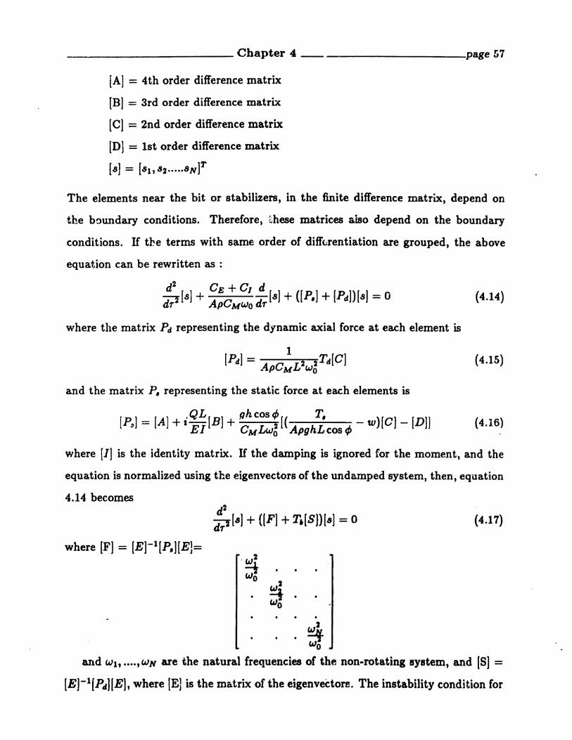
____________ Chapter 4 --------- page 57
[A] = 4th order difference matrix
IB] = 3rd order difference matrix
[C] = 2nd order difference matrix
[D] = 1st order difference matrix
[8] = (SI,82 •••••SN]T
The elements near the bit or stabilizers, in the finite difference matrix, depend on
the b!)undary conditions. Therefore) ~hese matrices also depend on the boundary
conditions. If tbe terms with same order of diffLrentiation are grouped, the above
equation can be rewritten as :
d2 CE + C1 dP [s] + A 0 -d [8] + ([p.] + [Pd])[S] = 0
T P MWo T
",here tIle matrix Pd representing the dynamic axial force at each element is
1[Pd] = A 0 £2 2Td[O]
P M Wo
and the matrix P, representing the static force at each elements is
(4.14)
(4.15)
.QL nh cos t/J T.[P3 ] = [A] + I EI [B] + OMLw~ [( Apgh£cos tP - w)[O] - [D]] (4.16)
where [1] is the identity matrix. If the damping is ignored for the moment, and the
equation is normalized using the eigenvectors of the undamped system, then, equation
4.14 becomes
where [F] = [E]-l[~.][EJ=
d2
p[s) + ([F) +T,[S})[s] = 0 (4.17)
.Wi.~
Woand WI, •••• ,WN are the natural frequencies of the non-rotating system, and [S] =
[EJ-1[Pd][E], where [E] is the matrix of the eigenveCtore~ The instability condition for

____________ Chapter 4 page 58
this system according to (23] is
(4.18)
where1
f1=(SijSji)2 (4.19)4WiW;
where Si; is the .:i-element of matrix [8]. The parameter f/ is the slope of the boundar)·
of the unstable regions. An increase in the slope will increase the size of the unstable
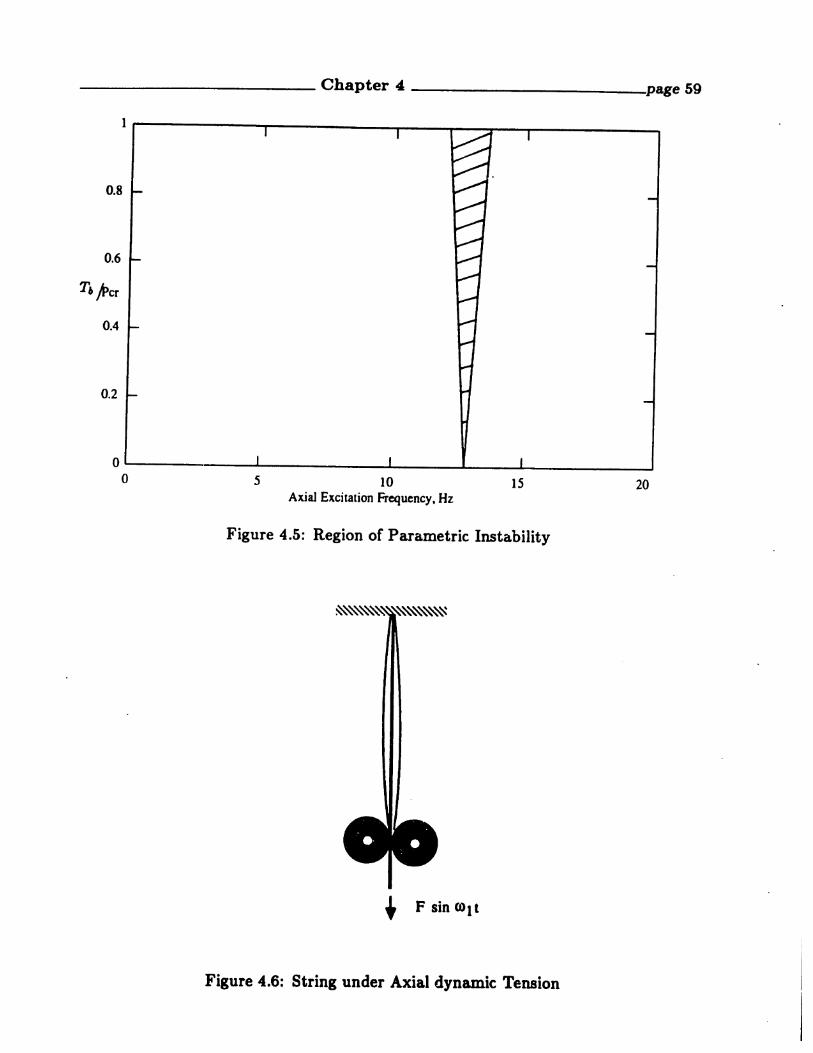
regions. Figure 4.5 shows an example of the unstable region for a pinned-pinned
Acrylic rod with ID=O inches , OD= 0.375 inches, and 3 feet long. The density of
the material is 2.68 s~~~s, and the Young's Modulus is 5.75 x 10⁷ psf. The figure is
plotted with axial excitation frequency W V8. amplitude of the dynamic axial force T,.
If the combination of wand Tb is inside the unstable region, the amplitude of bending
vibration ,,yill grow until it is ultimately restrainted by the borehole. In the example
given above, the unstable region was found for a condition with no external damping.
With no damping, the instability may be driven by an arbitrarily small excitation, Th•
The effect of damping is to raise the threshold of excitation which can produce the
instability. The greater the damping, the higher the threshold. A plot of the unstable
region will look similar as the one shown, except that it can not extend below the
threshold value. A detailed discussion of the effect of damping on the unstable region
can be found in [24]
4.6 String under Dynamic Axial Tension
As an aid to understanding parametric excited bending vibration of drill collars,
consider the string depicted in Figure 4.6. The string is shown passing through a
pair of pinch rollers, which is the lower boundary condition, and continues on to a
tens30n measuring device. H the string has a static compOIlent of tension To, and a
known mass per unit length, J.t, then the first natural frequency of the strillg can be
computed as,
------------ Chapter 4 -----------_page 59
201510Axial Excitation Frequency, Hz
5o~---..---"'------_.a.-..-_ ___..II.____a....._ ___'
o
0.8
0.4
0.2
Figure 4.5: Region of Parametric Instability
t F sin COt t
Figure 4.6: String under Axial dynamic Tension

____________ Chapter 4 page 60
WI = !~ To (4.20)L Jl
The undamped response of the string to an initial deflection in its first mode is simply
(4.21)
If one were to measure the dynamic ftuctuations in tension, which are caused by the
vibration at WI , the tension would be observed to vary at 2 times the vibration
frequency. The tension cO\11d be expressed as
(4.22)
(4.23)
The tension has a dynamic component at twice the vibration frequency. IT the process
was reversed and a tension with dynamic component of 2Wl wer~ applied at the end,
then the string will respond at its natural frequency, WI. This is a simple analogy to
the mechanism of parametric excitation of the bending vibration of the drill collars.
Expressed in drilling terminology, a dynamic component of the weight on bit is capable
of exciting bending resonances of the drill string ~t natural frequencies which are at
one half of the excitation frequency. A mud motor rotating a bit could parametrically
excite a non-rotating BHA.
4.7 Equation of Motion in a Rotating CoordinateSystem
Equation 4.7 describes a non-rotating BBA. The equation for a rotating beam
expressed in a rotating coordinate system is as follows:
82,' ar' a4r' as,'
ApOM 8t2 + (CE + 01 + i2w)at' +EI8z4 + iQ 8zS
a2r' or'+Apgh cos </>[(1' - z) 8z2 - 8z] - w2r' =0
where the prime in the expression r' denotes th~t the equation has not been put
in dimensionless form. The effect of the rotation is shown in the Figure 4.7. This

_----------- Chapter 4 ------- page 61
20155 10Axial Excitation Frequency, Hz
o I.- ----.l...-----L--....L.-------.....-I~-----------..
o
0.2
0.4
0.6
0.8
Figure 4.7: Region of Parametric Instability With Rotation Rate 2.4 Hz
example is plotted using the same data as in the earlier non-rotating case but now with
a rotating speed w of 2.4 Hz. It shows that the unstable region splits into two regions
The unstable response assol:iatt!d the higher frequency region was demonstrated using
a scale model as described in chapter 6.
4.8 Parametric Excitation of Bending Vibration aWith Borehole Constraint
Equation 4.7 describes the drill collar motion without the constraint of the bore
hole. This occurs possibly when the bore hole is nearly vertical. If the hole is slanted,
and stabilizers do not hold the collars in the center of the hole, they may lay against
the wall because of gravity. The section of the drill collars above the uppermost
stabilizer are most likely to exhibit such behavior. Figure 4.8 shows the coordinate
system used in the equation that describes the wall constraint. A detailed derivation

____________ Chapter 4 page 62
D
!::. =D-d
Borehole
Figure 4.8: Coordinate System
of the equation with wall constraint is presented in Appendix B. The equation of
motion with borehole constraint for the non-rotating case is:
82 '1 81 8 4,.., lJs'YApCM at2 + (CE +Cr) at + EIaz. + Q az3
, 8 2,.., 0' sin t/J
+Apghcost/>[(l - z) az2 - a) -I- Apgh~'Y =0 (4.24)
where. 6. is the borehole diameter minus the collar diameter, and '1 is an angle
measured with respect to the center of the hole between the static equilibrium point
of contact and the instantaneous point of contact between the drill collar and the wall.
'Y is both a function of axial position z and time. The definitions of the other symbols
are the same as those in equation 4.7. Following the same Dondimensionalization and
finite difference procedures, one can obtain the the matrix form of the equation
d2 01:+ 0 1 d QLdT2hl + ApCMwo dThl + (Alhl + El(Blbl
+p~co~t/>[(l_w)[Clhl- [D]bJl + ~hBi~~bl =0 (4.25)MWo MWo

(4.26)
____________ Chapter 4: page 63
where (A], [B), [el, [D] are defined in equation 4.7. H similar terms are grouped, then
d2 CE + C1 d
P b] + A C -d (7] + ([p.] + [Pd))[7] =0T P MWO. ".
where
[] [A] QL[B] pghcost/J[(~ _ )[0] _ [D]] ghsinc/>P, = + EI + C 2 , w + C 2A
M~ M~.
(4.27)
(4.28)
(4.29)
H the same normalizing ~. rocedure is taken, then equation 4.28 can be reduced to
d2
pb] + ([F] +T.[SDb] = 0
The instability condition for this system is the same as the case of no wall constraint,
which is
(4.30)
However, the natural frequencies Wi and w; are not necessarily the same as the case
without wall contact. Without wall contact, the mode shapes look sinusoidal about
the undeflected position of the straight beam. The mode shape lies entirely in a plane.
With wall contact, the mode shapes when projected on the wall still look sinusoidal.
But, as the beam deflects laterally, it must follow the curvature of the wall. In an
inclined hole this is resisted by gravity. In the same way as a frictionless mass will
oscillate in a circular shaped well due to gravity, the collar will also oscillate du~ only
to the restoring gravitational force. Compared to the bending stiffness of the collar,
this restoring force is negligibly small, except in the case of very low modes which
may have little restoring force due to beam stiffness. This is especially true for the
modes whose natural frequencies are reduced due to large compressive loads in the
BRA. In other words, the presence of the wall may increase the natural frequency
of the modes that are likely to be sensitive to buckling effects in the BHA~. The
unstable regions are indicated in Equation 4.30 The length of the drill collars above
the uppermost stabilizer can be several hundred feet. Therefore, the modal density

_____________ Chapter 4: -------- page 64
(the number of modes per unit increase in frequency) of the bending vibration may
get quite high, resulting in overlapping regions of instability. So, [19] introduces a
term called severity, which is the same as '1 in the above equations and was defined
previously by for the case without wall contact, and is givell again here.
1S--8·· -2
'7 = 8everity = ( " ")4wjw;
(4.31)
where Si; is the .:i-element of matrix [8]. But, with high mo~al density, it is difficult to
plot the unstable regions, which may correspond to 20 or 30 modes that fall into the
frequency range at which the collar would rotate. Instead of attempting to plot the
regions of unstable response, we can plot the parameter,., versus the frequency, Wi+W;.
This parameter gives the relative sizes of the unstable regions. So, '1 can be thought
of as an indication of the likelihood of operating in the unstable region. The larger
the opening of the unstable region, the more likely the drill string will encounter
it. Therefore, the peaks in the severity versus frequency plot give information on
the excitations frequencies that are likely to drive the collars above the uppermost
stabilizer into unstable responses. One example of this calculation is shown in Figure
4.10. The inputs for this calculation are given in Figure 4.9 for a BHA with no
stabilizers. The confirmation of this prediction with field or lab model has not yet
been obtained and published. But once confirmed, one engineering application of
this result is to avoid these peaks in the actual drilling conditions. For example, if
a tricone bit is used for the drilling, strong axial excitation occurs at 3 and 6 times
the rotation rate. These axial excitation frequencies should not be the same as -the
frequencies of high severity peaks, in order to avoid potential high bending responses.
. Equation 4.30 shows that the width of an instability region is proportional to both
the severity and the dynamic fluctuations in the weight on bit, T.. One interpretation
is that the severity is a measure of the instability risk per unit of excitation force, T•.
The severity calculation includes the longitudinal dynamic properties of the entire
drill string. The severity is likely to be worse at frequencies wh.ich correspond to

_____________ Chapter 4 page 65
longitudinal resonances.
All of the foregoing discussion was based on the assumption that the drill collar
was not rotating and that the bit forces were the result of operation with a mud
motor. Rotation introduces many potential complications which are not addressed
in this thesis. However, the argument has been made but not proven, that the wall
contact constraint nullifies the effects of the rotation on the natural frequencies, Wi
and w;, which are to be included in the severity calculation. Therefore, the results
are the same as in the non-rotating case.
However, the examination of the Shell-NL downhole data taken in experiments
described in [52] shows that the dynamic response in bending close to the bit is usually
a very complex superposition of many simultaneous phenomena. The prediction of the
instabilities under such circumstances may be much more difficult than describe here.
In chapter 7, there is one example with evidence of parametrically excited bending
vibration, thus, verifying the existence of the phenomena for a BHA. with stabilizers
in a regioll without wall contact.

------------- Chapter 4 -----------__page 66
Damping "4-- Spring k=200000 Ibs/ft
.- Mass 118 slugs
Drill pipe (Aluminum)
OD= 4.6"ID= 3.6"
Density = S.8 slugs/ft3
Damping = I.S3 Ibf-scc/ft 2 (axial)
•
Drill Collar
OD=7.81"ID=6.5"Hole Diameter = 9" 3Density = 15.2 slugs/ft 2Damping = 2.168 Ibf-sec/ft (axial)
•..--Bit
1130'
711.5'
1
Figure 4.9: Inputs for the Severity Calculation
0.01
0.008
0.006
0.004
Hz
oL.::::~:::IIIIC~CL..L..L.J--l.~:::=.c:::~~c::..~~--.......:::::::~-.;;::a------
o 5 10 IS
(Wi +wj)/21f
Figure 4.10: Severity versus Frequency Plot
0.002

Chapter 5
Rubbing of the Drill Collars
The drill string is designed to rotate, from 40 to about 100 RPM for conventional
tri-cone and PDe bit drilling. As the drill collar rotates, whirling motion can be
introduced. Whirling is simply the centrifugally induced bowing of the drill collar.
Consider a crill collar in Figure 5.1H the center of the gravity of the drill collar
in not initially located precisely on the axis of rotation, then, as the collar rotates,
a centrifugal force acts on the center of gravity, causing the collar to bend. The
magnitude of the force is proportional to the mass of the collar, the square of the
rotation rate, and the initial eccentricity of the mass center to the axis of rotation
(usually the center of the hole). The initial eccentricity of the drill collar can result
from several causes, including an initially bent drill collar, or sag due to an inclined
borehole and gravity, or an eccentrically loaded weight on bit. This eccentricity can
result in dynamic imbalance as the collar starts to rotate.
Whirling has been long known to occur in a destructive form in rotating machin
ery when the rotation rate of the shaft equals the natural frequency of that shaft
in bending. When this happens, the machine is known to be operating at a critical
speed. There is. an enormous established literature on the subject of whirling of ma
chines, such as turbine engines, axial flow compressors, and generators. An excellent
tutorial on the subject may be found in reference [34], which presents a mathematical
description of the simple whirling of a rotating shaft.
A great deal of effort and money is spent on balancing shafts and on developing
67

_____________ Chapter 5 ---------- page 68
Stabilizer
~it
n : Whirling Speed
Figure 5.1: A Whirling Drill Collar
operating guidelines for machinery, so as to prevent serious whirling. This is generally
not done with drill strings. One reason is that drill strings operate in the confinement
of the borehole. Whirling does not generally result in precipitous failures of drill
collars, because deflection amplitudes are limited by wall contact. There are, however,
undesirable consequences of drill collar whirling behavior, not necessarily recognized
in the drilling industry. One is abrasion of the surface of drill collars caused by rubbing
on the wall.
The presence of the wall imposes displacement constraints on the bending and the
whirling motion of the drill collar. Wall constraints not only limit the displacement
of the collar, but also increase the stiffness of the collar if the collar comes in coniact
with the wall. There are several possible kind of rubbing behavior
• partial rub
• synchronous full annular rub
• ba~kward full annular rub
____________ Chapter 5 --------.- page 69
Partial rub is characterized by the occasional contacts between the collar and the
wall. If the collar maintains constant contact with the wall, the term. "full annular
rub" is used. It can be either in a forward or a backward direction with respect to
the direction of the collar rotation. From an engineering point of view, synchronous
rub, in which the same side of the collar is in constant contact with the side of the
borehole, is the probable cause when a collar comes out of the hole worn flat in one
place. In pure backward rub, the drill collar rolls without slipping on the inside of the
hole in a direction opposite to the surface rotation rate (hence the name "backward
whirl"). Your eye, if it could follow backward whirl, would see the center of the drill
collar moving around the hole at a frequency much higher than the rotation rate of
the drill collar itself. This phenomenon does not cause substantial surface abrasion,
because there is little, if any, relative velocity between the drill collar and the wall.
High frequency stress cycles, caused by bending of the drill collar, occur at many
times the rate of rotation and may possibly lead to connection fatigue failure. These
phenomena are explained in more detail in the following sections.
5.1 Kinematics of Whirling
The relative tangential slip velocity V between the drill collar and the borehole
. wall is given in chapter 2, as reproduced here:
(5.1)
The tangential slip velocity is a measure of the amount of abrasion. experienced by
the drill collar on the wall. This velocity may vary from zero under conditions of
perfect backward whirl with no slip to a maximum of R60 under conditions of forward
synchronous whirl. For fixed drill collar rotation rate w, the tangential slip velocity
V is. a linear function of whirl rate o. Figure 2.2 in chapter 2 shows this linear
relationship, and also indicates values of n where forward and backward whirl occur.
Backward whirl occurs for values of n less than- zero. Backward whirl without slip

____________ Chapter I) - page 70
occurs when V is zero. By requiring the tangential slip velocity to be zero, equation
5.1 may be used to solve for the whirl rate 0., which is defined as the condition of
backward whirl without slip:Wen6 = (5.2)14-Rc
Backward whirl with slip occurs for values of 0 algebraically greater than O. but
less than zero. No whirl occurs if n =0 (i.e., the drill collar rotates but does not whirl
around the hole center). Forward whirl with slip occurs for values of 0 greater than
zero. The special case of forward synchronous whirl occurs when the whirl rate is
equal to the drill collar rotation rate, n = w. Drill collar whirl is considered .unlikely
for n < Ob and n > w, since "negative" wall friction would most likely be necessary
to drive the whirling motion.
The whirl ratio is defined as the ratio of the actual whirl speed to the backward
whirl speed with no slip:n
s =-- (5.3)Ob
Substitution in equation 5.1 leads to the following useful variation for the expression
for tangential velocity :
(5.4)
5.2 Partial Rubs
Partial rubbing is characterized by the occasional impact between wall and the col
lars. The motion of the drill collars before the first impact is most likely synchronous
whirl. The normal impact force will be small in comparison with WOD because of
the the relatively small clearance between wall and the collars. After the impact, the
collar responds with lateral and torsional motion. The direction of rebound depends
on t~e whirling velocity of the drill collar at the instance of impact. It either follows
the original whirling direction or reverses into backward whirl. ~{U8ZYD8ka (37) inves
tigated the problem of partial rotor to stator rub and concluded that, partial rub will
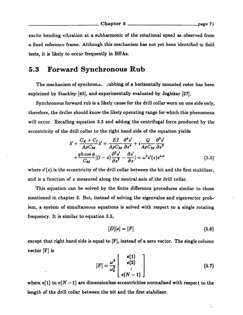
(5.5)
____________ Chapter 5 ------- page 71
excite bending vibration at a subharmonic of the rotational speed 88 observed from
a fixed reference frame. Although this mechanism has not yet been identified in field
tests, it is likely to occur frequently in BHAs.
5.3 Forward Synchronous Rub
The mechanism of synchron\l\. :ubbing of a horizontally mounted rotor has been
explajned by Stackley (45], and experimentally evaluated by Joglekar (27).
Synchronous forward rub is a likely cause for the drill collar worn on one side only,
therefore, the drIller should know the likely operating range for which this phenomena
will occur. Recalling equation 3.3 and adding the centrifugal force produced by the
eccentricity of the drill collar to the right hand side of the equation yields
.., CE + C1., E.l 848' . Q ass'
S + ApCM S + ApCM 8z. + I ApCM 8zs
ghcostP[(l ) 82s' as'] 2,() iwt+ CM - z 8 Z2 - 8 z = w e z e
where e'(z) is the eccentricity of the drill collar between the bit and the first stabilizer,
and is a function of z measured along the neutral axis of the drill collar.
This equation can be solved by the finite difference procedures similar to those
mentioned in chapter 3. But, instead of solving the eigenvalue and eigenvector prob
lem, a system of simultaneous equations is solved with respect to a single rotating
frequency. It is similar to equation 3.5,
[D][s] = [F] (5.6)
except that right hand Bide is equal to [F), instead of a zero vector. The single column
vector (F] ise(l)e(2)
(5.7)
e(N - 1)where e(l) to e(N -1) are dimensionless eccentricities normalized with respect to the
length of the drill collar between the bit and the first stabilizer.

------------ Chapter 5 --------- page 72
Figure 5.2 shows the displacement of the collar at one quarter and one half the
length. trhe inputs for this example are shown in Table 5.1.
Table 5.1: Inputs for the Example
100
o
7.5
2.81
10000.
3. 2. 200
10
12
0.8
30000
1.0
0.1 O.
0.1 O.
0.1 O.
0.1 O.
1.
4.32E+09
L , Ft, Total length of the collar between the bit and the first stabilizer
Ci, Lbs/{Ft/sec)/Ft of pipe, Internal damping
OD, Inches
ID, Inches
Q , Lbs.Ft, Torque
Initial, increment, and ending value of rpm
Phi, Degrees, Slant angle of the borehole
RHOMUD, Lbs/Gallon, Density of the mud
Ce, Lbs/{Ft/sec}/Ft of pipe, External damping
JJbs, Weight on Bit
N Segments (type 4M-l)
C (O=Pinned, l=Clamped)
e'l, Eccentricity of Lower Quarter of the drill collar
Magnitude in inches, Phase in degrees
e'2 Eccentricity of 2nd Quarter
e'3 Eccentricity of 3rd Quarter
e'4 Eccentricity of the Top Quart of the drill collar
added mass coefficient of the mud
Young's Modulus of the collar material
The displacements at quarter and half points on the collal are plotted assuming
no wall contact. Normal operating speeds for a 100 foot pendulum BHA are from 40
RPM to 200 RPM. This range includes the natural frequencies for the first two bending

____________ Chapter 5 -----__page 73
2-------r----------,r---------,---------,
1.5
Inches
0.5
Displacement at Half Length
oLL~--.l-----...L:i-:.~======:::t=======---...:::Jo 50 100 150 200
RPM
:F'igure 5.2: The Displacement at Quarter Length and Half LeIlgth above the Bit
modes. The first mode shape is a half sine wave, and the maximum displacement is at
the half length point. The second mode shape is a full sine wave, and the maximum
displacement is near the quarter length point. If the maximum displacement of the
collar is less than the clearance, then, no rub is initiated, and the possible whirling
motion of the drill collar is forward synchronous whirl. IT the maximum displaceloent
equals or exceeds the clearance, the rub is initiated. The clearance limit in Figure
5.2 would be indicated as a horizontal line, whenever the predicted amplitude crosses
this limit, rub of some kind will result.
According to Stackley, the frequency range of the rubbing is likely to be wider
than the frequency range in which the collar displacement exceeds the clearance, due
to the modification of the collar stiffness as it touches the wall of the borehole. No
attempt has been made in this thesis to predict the extension of the RPM range that
the collar engages in forward synchronous rubbing. The analysis here gives only the
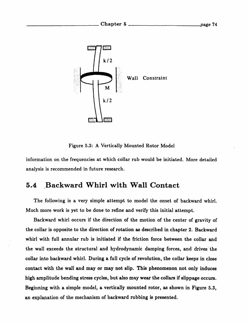
____________ Chapter 5 --------- page 74
Wall Constraint
Figure 5.3: A Vertically Mounted Rotor Model
information on the frequencies at which collar rub would be initiated. More detailed
analysis is recommended in future research.
5.4 Backward Whirl with Wall Contact
The following is a very simple attempt to model the onset of backward \vhirl.
Much more work is yet to be done to refine and verify this initial attempt.
Backward whirl occurs if the direction of the motion of the center of gravity of
the collar is opposite to the direction of rotation as described in chapter 2. Backward
whirl with full annular rub is initiated if the friction force between the collar ~d
the wall exceeds the structural and hl'drodynamic damping forces, and drives' the
~ollar into backward whirl. During a full cycle of revolution, the collar keeps in close
contact with the wall and mayor may not slip. This phenomenon not only induces
high amplitude bending stress cycles, but also may wear the collars if slippage occurs.
Begil1ning with a simple model, a vertically mounted rotor, as shown in Figure 5.3,
an explanation of the mechanism of backward rubbing is presented.

____________ Chapter 5 -------- page 75
N
Borehole
+ Stiffness Force
Figure 5.4: Force Diagram of Backward Rubbing
The model shown in Figure 5.3 has a disk of mass M, and a massless shaft with
lateral stiffness K. This model is enclosed by an infinite rigid casing with fluid in it.
Figure 5.4 shows the forces involved in the backward whirl. 1.'he equation of motion
describing this mechanism in the tangential direction is
. and the force equilibrium in the radial direction is
where
M : mass of the rotor
rc : radial clearance
n : whirling speed of the rotor
D : damping forces
J.I, : friction coefficient between wall and the collar
(5.8)
(5.9)

____________ Chapter 5 ------- page 76
N : normal force acting on the wall by the collar
R : portion of the normal force acting on the wall due to
the coupling between the axial force and the curvature
of the BHA
W n the first natural frequency of the system
If we assume that the damping is caused mainly by hydrodynamic mechanisms, D
can be expressed as
(5.10)
where Pm is the density of the surrounding fluid, and CD is the hydrodynamic drag
coefficient, and r is the radius of the disk. Note that the hydrodynamic drag coefficient
ranges from 0.2 to 2.0 for cylinders in an unbounded fluid. The correct values for these
condition is not known. Substituting the expression for N into the radial direction,
we have
where
(5.11)
p,Mrc + PmCDrr~
Mrc
- p,R + p,Mrcw~
Mrc
(5.12)
(5.13)
H equation 5.3 is substituted into equation 5.11, and taking the whirl ratio, ~6' as
the dependent variable, then
(5.14)
This equation can be numerically integrated in the time domain to show the behavior
of this equation. Following is an example with a hole diameter of 8.75 inches, a collar
diameter of 7 inches, and a ratio of rotation rate. to natural frequency of 1.0. The
damping ratio and friction coefficient are assumed to be 0.05 and 0.3, respectively.
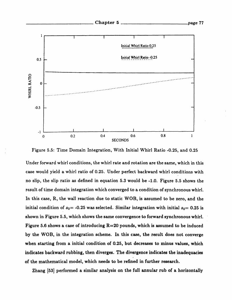
I
0.5 -
I I
Initial Whirl Ratio 0.25
Initial Whirl Ratio -0.25.................
I
-
o~
.................... .
·0.5 ~
......................................
. ................. -
-
-1o
I
0.2
I I
0.4 0.6SECONDS
I
0.8
Figure 5.5: Time Domain Integration, With Initial Whirl Ratio -0.25, and 0.25
Under forward whirl conditions, the whirl rate and rotation are the same, which in this
case would yield a whirl ratio of 0.25. Under perfect backward whirl coIiditiollS with
no slip, the slip ratio as defined in equation 5.3 would be -1.0. Figure 5.5 shows the
result of time domain integration which converged to a condition of synchronous whirl.
In this case, R, the wall reaction due to static WOB, is assumed to be zero, and the
initial condition of 80= -0.25 was selected. Similar ultegration with initial 80= 0.25 is
shown in Figure 5.5, which shows the same convergence to forward synchronous whirl.
Figure 5.6 shows a case of introducing R=20 pounds, which is assumed to be induced
by the WOB, in the integration scheme. In this case, the result does not converge
when starting from a initial condition of 0.25, but decreases to minus values, which
indicates backward rubbing, then diverges. The divergence indicates the inadequacies
of the mathematical model, which needs to be refined in further research.
Zhang [53] performed a similar analysis on the full annular rub of a horizontally

______________ Chapter 5 ------------__page 78
0.5
-0.5
-1o 0.2 0.4 0.6
SECONDS0.8
Figure 5.6: Time Domain Integration, With Initial Whirl Ratio 0.25, and AdditionalWall Reaction
mounted flexible rotor system, and concluded that the conditions when the backward
rub occurs are dependent on the initial contact velocity between the collar and the
wall. Detailed experimental work is needed to verify this result.
The discussion presented above describes the collar motion by assuming the collar
is in constant contact with the wall, and the equation of motion describing the forces
in radial and tangential directions is derived under this assumption. This analysis
gives only a preliminary mathematical model· for the prediction of whirl conditions.
Further refinements in prediction techniques and experimental work are left as future
research topics.

Chapter 6
Laboratory Experiments
To demonstrate the validity of the theories detailed in previous ch~pters, experi
ments were carried out on a scale model in the laboratory. These experiments were
conducted also with the purpose of better understanding the phenomena of whirling
and coupling mechanisms. From these experiments, we also learned to recognize what
these phenomena look like when observed in a rotating coordinate system, such as
with a downhole tool.
6.1 Dimensional Analysis
Before proceeding with the scaled model experiments, a dimensional analysis was
performed to estimate a suitable model.
In dimensional analysis, a group of parameters that reflect the dynamics of the
system are selected to be modeled. For bending vibration of Bottom Hole Assem
blies, the following 10 parameters were chosen and their relationship is stated by the
following equation :
where
s = 1(1, d, D, E, P, Pm, T, g, 4>, n)
s : lateral displacement of the drill collar
I : characteristics length of the drill collar
d: drill collar outside diameter
79
(6.1)

____________ Chapter 6 --- page 80
D : diameter of the bore hole
~ E : Young's Modulus of the collar material
p, Pm : density of the collar and mud
T : weight on bit
g : gravity
4> : slant angle of the bore hole
n : rotation speed of the collar
If the independent parameters I, p - Pm, and E were selected, they can be arranged
into 7 independent dimensionless groups. Let's denote length by L, mass by M, and
time by S, then 1, p, and E will have the following units:
I: LM
p: IJM
E: S2L
Using Buckingham 1(" method, a nondimensional relationship can be found for equation
6.1:
T= /·(6b 62,6s,6.,66) (6.2)
where
61d
(6.3a)- -I
(J2D
(6.3b)- -I
8sT
(6~3c)- 12E
64E
(6.3d)-gl(p - Pm)
1
86IO(P - Pm)2 (6.3e)- E
66 - tP (6.3f)
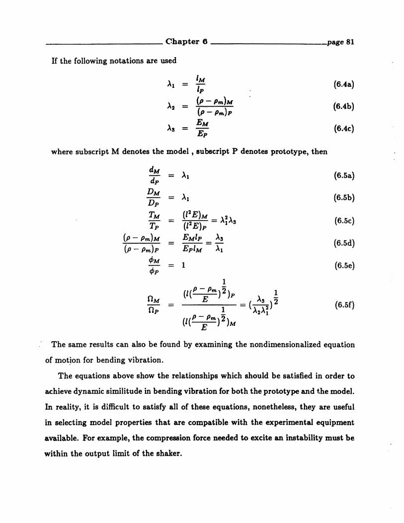
____________ Chapter 6 _
If the following notations are used
Al'
M- lp
A2(p - Pm)M
- (p - Pm)P
AsEM
- -Ep
page 81
(6.4a)
(6.4b)
(6.4c)
where subscript M denotes the model, subscript P denotes prototype, then
dM Al (6.5a)dp
-
DM Al (6.5b)- -Dp
TM (1 2E)M = A~AS (6.5c)- - (1 2E)pTp
(p - Pm)M EMlp ~s(6.5d)
(p - Pm)P- --
EplM Al<PM
1 (6.Se)- -tPP
1
(I(P -;m)"2)p 1OM = ( A\)"2 (6.5£)- -Op 1 A2Al
(I(P -;m)"2)M
The same results can also be found by examining the nondimensionalized equation
of mot~on for bending vibration.
The equations above show the relationships which should be satisfied in order to
achieve dynamic similitude in bending vibration for both the prototype and the model.
In reality, it is difficult to satisfy all of these equations, nonetheless, they are useful
in selecting model properties that are compatible with the experimental equipment
available. For example, the compression force needed to excite an instability must be
within the output limit of the shaker.

____________ Chapter 6 ------- page 82
6.2 Model Selection
From preliminary analysis, the plastic material, acrylic, was selected. The density
of this material is about 2.48 slugs per cubic foot, and the Young's modulus is about
380,000 psi. The sample chosen for the experiment was a rod, 3.25 feet long and 0.25
inches in diameter. It was used to approximately model a 60 foot drill collar with
mass density of 15.2 slugs per cubic foot, Young's modulus of 30,000,000 psi, and
with drilling mud of 8.8 pounds per gallon. The value for ~1 is 0.054, >t2 is 0.188,
and As is 0.0126. With these numbers, we can calculate the ratio of weight-on-bit,
which is 0.0000367, between model and prototype. So, if we are simulating a dynamic
WOB of 10,000 pounds, the dynamic force needed for the experiment is only about
0.3 pounds, which is within a output range of a relatively small shaker. The model
to prototype ratio of rotational speeds is 4.8, as determined using the same values of
AI, A2' and A3. If the operating speed of the actual drill string is 60 to 200 RPM; then,
the corresponding speed in the model would be 288 to 960 RPM (4.8 to 16 RPS). This
range of speed can be achieved by using a very simple variable speed electric motor.
Note that because of the material chosen for the experiment and the limitations of
the experimental equipment, the relation in equation 6.5 did not hold exactly for the
this experiment. Nonetheless, we were a~le to make, for example, the rotational speed
close to the modelling criteria. In the experiment, a rotational speed of 2.5 Hz was
used. Also the shaker used in the experiment ca~ put out a few pounds of force, and
was capable of 0.3 pounds required by the modelling.
6.3 Setup of the Experiment.
Figure 6.1 is the layout of the experiment. A supporting frame 5 feet long was used
80 that experiments could be performed at any angle of inclination. An electric motor
was 'placed near the top of the supporting frame. This motor could be operated from
1.5 to 25 revolutions per second. A slip ring was ~ttached to the motor's shaft, and

____________ Chapter 6 page 83
Supporting Frame
~Motor
Slip Ring
Universal -------.......Joint
3.5'
ImpedenceHead
Shaker
Figure 6.1: Layout of the Experiment
a universal joint was connected to the other end of the slip ring. Then, the universal
joint was connected to the testing rod. The universal joint was used here to provide
a pinned-like boundary condition for the bending vibration at the top of the testing
rod. A pinned boundary condition was accomplished at the bottom and by running
a metal point in a small hole. The purpose of the slip ring was to provide for the
connection between the strain gages on the shaft and the strain gage amplifier. The
slip ring created about 50 micro-ohms of noise; well below the problem level. A B&K
mini-shaker simulating the forces of bit-rock interaction was placed at the bottom.
It was driven by a power amplifier and a function generator. Two strain gages were
installed 90 degrees apart to measure two axes of beDding as shown in figure 6.2. The
slip ring was used to carry the gage signals from the rotating shaft to a strain gage
amplifier. A WR impedance head was placed between the shaft and the shaker to
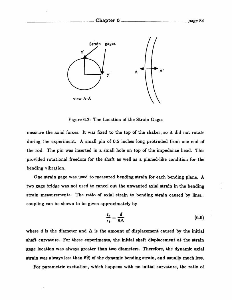
____________ Chapter 6 -------- page 84
Strain gages
y'
view A-A'
A
Figure 6.2: The Location of the Strain Gages
measure the axial forces. It was fixed to the top of the shaker, so it did not rotate
during the experiment. A small pin of 0.5 inches long protruded from one end of
the rod. The pin was inserted in a small hole on top of the impedance head. This
provided rotational freedom for the shaft as well as a pinned-like condition for the
bending vibration.
One strain gage was used to measured bending strain for each bending plane. A
two gage bridge was not used to cancel out the unwanted axial strain in the bending
strain measurements. The ratio of axial strain to bending strain caused by linen .. '
coupling can be shown to be given tl.pproximately by
(6.6)
where d is the diameter and 6. is the amount of displacement caused by the initial
shaft curvature. For these experiments, the initial shaft displacement at the strain
gage location was always greater than two diameters. Therefore, the dynamic axial
strain was always less than 6% of the dynamic bending strain, and usually much less.
For parametric excitation, which happens with no initial curvature, the ratio of

____________ Chapter 6 --- page 85
dynamic axial strain to dynamic bending strain is given by
Ea 8PL2
E6 - 1fEcfA
where
P = dynamic axial force
L = length
E = Young's Modulus
d = diameter
A = midspan bending deflection in the first mode
(6.7)
For a bending vibration amplitude of one diameter and an axial load of 0.3 pounds,
this ratio for the experiment was less than 8%. At resonance, the respon£;e amplitude
was much larger, and this ratio was proportionately smaller. The contamination of
the bending strain measurements by the axial strain was not a significant factor in
the conclusions of the tests.
6.4 Data Acquisition
An IBM AT compatible machine with a MetraByte Das-16 AID Board was used
to sample the signals. The AID software used was capable of writing digitized dat"a
directly onto the hard disk. Each data point is written in two byte ;nteger format. The
maximum sampling rate of this system is around 5K Hz. Two stain gages signals and
the signals from the impedance head, which are force and acceleration, were taken
during the experiments. The sampling frequency was fixed at 200 Hz per channel
throughout the experiments.
Figure 6.3 shows the connections between the transducers and the computer.
6.5 .Experimental Procedures
The first na.tural frequency of the non-rotating shaft varied from 3.5 to 3.9 Hz
depending on the amount cf mean (constant) component of comprp.JJsive axial force,

____________ Chapter 6 page 86
Slip Ring
Shaft
Strain GageAmplifier
ChargeAmplifier
IBM AT withMetrabyteDas-16 Board
Impedance Head
Figure 6.3: Signal Path of the Experiment
and upon the mean curvature. A constant axial force was required to support the
weight of the shaft as well as to prevent any bouncing of the lower bearing point
in the retaining hole. Increase in either axial force or curvature ( such :J.S due to
whirling) reduced the natural frequency. Of course, the same is also true in a real
drill collar. During the rotating experiments, the mean curvature changed in an
uncontrollable way due to the combined effects of whirling and mean axial force, thus
causing the equivalent non-rotating natural frequency to vary from 3.5 to 3.9 Hz. For
the prediction calculations shown here, an average value of 3.7 Hz is used. Resonance
frequencies under actual conditions varied by a small amount due to changes in mean
curvature and mean axial force.
The .experiments were carried out by holding the rotation speed constant at 2.5
Hz, and varying the shaker frequency from 1 to 15 Hz in increments of about 1 Hz.
This sweep test allowed the estimation of the correlation between the input force and

____________ Chapter 6 ----------__page 87
the bending response.
6.6 Discussion of the Results
The specific purpose of the experiments was to observe and describe both linear
coupling between axial force and bending vibration and parametrically excited bend
ing vibration. Before conducting the experiments, we understood in a mathematical
sense that vibration could result, but we would have been hard pressed to clearly
describe it. The experiment had a significant self education component.
In chapter three, it was predicted that resonances at natural frequencies when
experienced on a rotating beam would occur at frequencies which are different than
that predicted for a non-rotating beam. The predicted natural frequencies as observed
on the rotating beam are given by the following equation in (rad/sec)
or expressed in Hz as
W; = Wn - W
w~ = Wn + W
(6.8a)
(6.8b)
(6.9a)
(6.9b)
wher~ ~ is the rotation rate in Hz and In = ~; is a bending natural frequency for
a non-rotatiIlg beam. These equations indicate that as the beam begins to rotate, the
natural frequencies bifurcate in frequency. Resonant conditions no longer correspond
to excitation at the non-rotating natural frequency In but occur when the excitation
corresponds to either of the two bifurcated frequencies given above.
The bifurcated natural frequencies correspond to mode shapes which are seen as
orbits in the rotating frame. In other words, the beam not only bends into the mode
shape as expected in the non-rotating case but also makes elliptical orbits about

_____________ Chapter 6 ------ page 88
its mean radial position. At any section of the beam, the center of gravity of the
section will appear to move in an elliptical or circular path. The direction of the
orbit is different for the two bifurcated modes. The f: mode represents orbits in the
direction of the rotation and the I; mode represents motion opposite to the rotation
direction when I; is positive, and in the direction of rotation when it is negative.
An objective of the experiment was to visualize these motions, as well as test out the
predictions of linear coupling and parametric excitation.
As discttssed earlier, the natural frequency of first bending mode was approxi
mately 3.7 Hz. The rotation speed of the model was 2.5 Hz. So the bifurcated
natural frequencies with respect to t,he rotating reference frame were expected at:
I; = 3.7 - 2.5 = I.2Hz
f; = 3.7 + 2.5 = 6.2Hz
Under synchronous whirl conditions at the natural frequency, the shaft bows out to a
deflected position and stays there. Any point on the shaft stays at the same distance
relative to the center of the hole, and in the moving reference frame, does nClt appear
to move. In the fixed reference frame, a proximity probe would see large vibration
at the shaft rotating speed. Depending on the reference frame of the observer, the
vibration frequency takes on different values. The one most important to drilling
is the one seen in the rotating reference frame, because this is the frame in which
measurements are made OD. Figure 6.4 shows the force spectra as measured by the
impedance head for the control case that the shaft was not rotating. Each spectrum in
the stack was generated with the control signal to the shaker at different frequencies
beginning at 3 Hertz, then, progressing up to 9 Hertz in steps of 1 Hertz. The shaker
frequency is indicated on the right hand side of the plot. Each spectrum shown in
the plot in the force spectrum was observed by the impedance head, when the control
signal to the shaker was at a single frequency. For each spectrum the major peak,
measured on the horizontal axis, should correspond to the frequency indicated on the
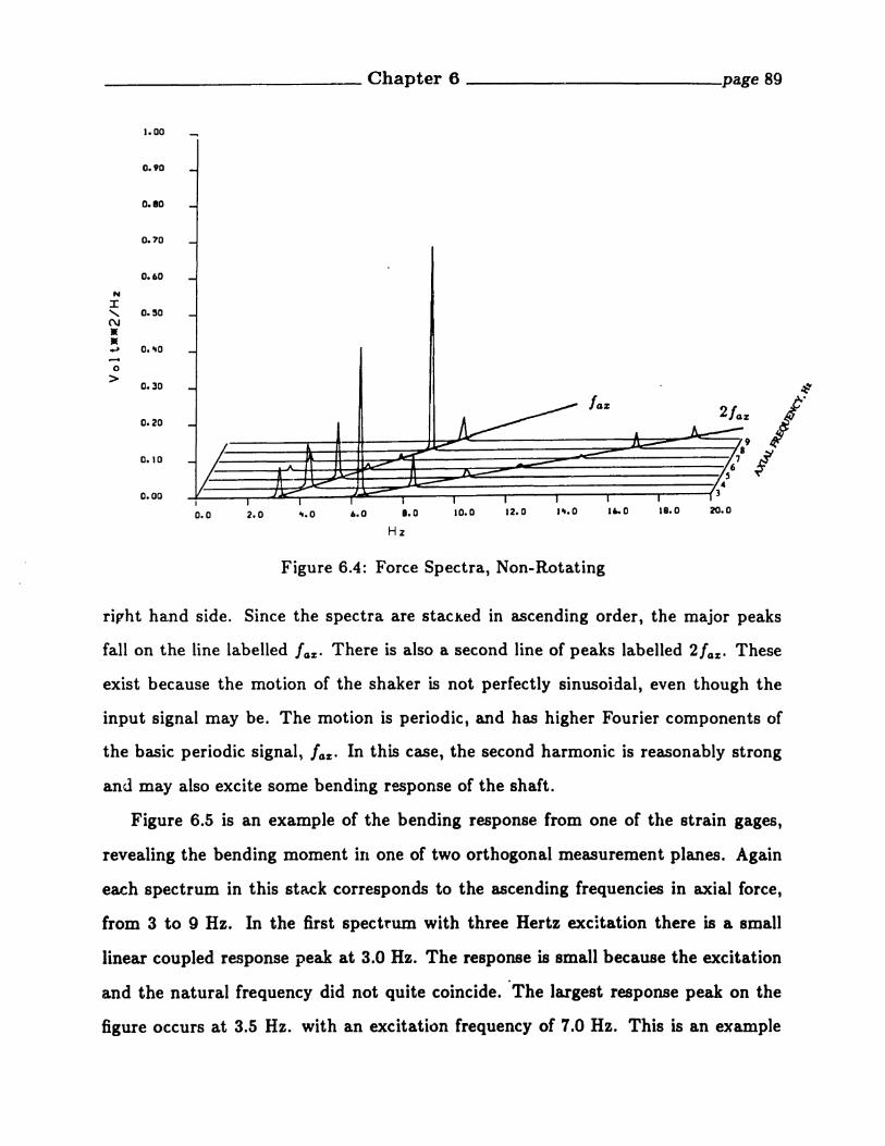
______________page 89
20.018.01... 01... 012.010.01.0
Hz'.0... 02.0
,If
2/0%
,----~__1.~---_H_::~~-------'1t:::::;::::---.----..-~
/------A-~~~~---~..--.------t I
Figure 6.4: Force Spectra, Non-Rotating
rirht hand side. Since the spectra are stacKed in ascending order, the major peaks
fallon the line labelled faze There is also a second line of peaks labelled 2!az. These
exist because the motion of the shaker is not perfectly sinusoidal, even though the
input signal may be. The motion is periodic, and has higher Fourier components of
the basic periodic signal, fGze In this case, the second harmonic is reasonably strong
and may also excite some bending response of the shaft.
Figure 6.5 is an example of the bending response from one of tIle strain gages,
revealing the bending moment in one of two orthogonal measurement planes. Again
each spectrum in this stack corresponds to the ascending frequencies in axial force,
from 3 to 9 Hz. In the first spectrum with three Hertz excitation there is a small
linear coupled response peak at 3.0 Hz. The response is small because the excitation
and the natural frequency did not quite coincide. "The largest response peak on the
figure occurs at 3.5 Hz. with an excitation frequency of 7.0 Hz. This is an example

____________ Chapter 6 - page 90
10.0 12.0 .".0 U•• O 18.0 20.0
Figure 6.5: Bending y' Spectra, Non-Rotating, Parametric Resonance
of a parametric excitation of the first mode of the non-rotating shaft which has an
approximate natural frequency of 3.7 Hz in response to an axial excitation at twice
the response frequency. Recall that from Figure 4.5 the Ullstable region is a band of
excitati~n frequencies centered on 2fl.
Moving on, a rotat\ng example is shown in Figure 6.6. This figure is again a
cascade sequence of the spectra of the force signal. But, in this case the motor was
running and the rotation rate was at 2.5 Hertz. Each successi\"e plot in this cascade
was taken when the axial force signal was set at successively higher frequencies from 1
to 15 Hertz. '.I.-here is a small straight line of peaks at 2.5 Hertz. This is at the rotation
ra·te and is likely caused by irregularities in the thrust bearing or the universal joint,
causing a once per revolution perturbation, which can be seen in the force signal. It is
helpful because it shows that the beam was indeed rotating and reveals the rotation
frequency. There are many other peaks in this spectral plot, but the most important
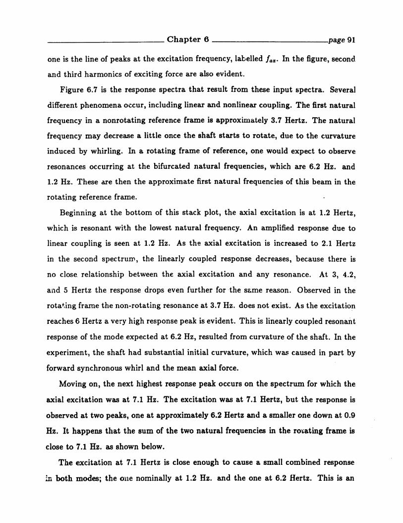
____________ Chapter 6 --- page 91
one is the line of peaks at the excitation frequency, labelled faze In the figure, second
and third harmonics of exciting force are also evident.
Figure 6.7 is the response spectra that result from these input spectra. Several
different phenomena occur, including linear and nonlinear coupling. The first natural
frequency in a nonrotating reference frame is approximately 3.7 Hertz. The natural
frequency may decrease a little once the shaft starts to rotate, due to the curvature
induced by whirling. In a rotating frame of reference, one would expect to observe
resonances occurring at the bifurcated natural frequencies, which are 6.2 Hz. and
1.2 Hz. These are then the approximate first natural frequencies of this beam in the
rotating reference frame.
Beginning at the bottom of this stack plot, the axial excitation is at 1.2 Hertz,
which is resonant with the lowest natural frequency. An amplified response due to
linear coupling is seen at 1.2 Hz. As th~ axial excitation is increased to 2.1 Hertz
in the second spectrum, the linearly coupled response decreases, because there is
no close. relationship between the axial excitation and any resonance. At 3, 4.2,
a11d 5 Hertz the response drops even further for -the sC.me reasoD. Observed in the
rota+,ing frame the non-rotating resonance at 3.7 Hz. does not exist. As the excitatio~
reaches 6 Hertz a very high response peak is evident. This is linearly coupled resonant
response of the mode expected at 6.2 Hz, resulted from curvature of the shaft. In the
experiment, the shaft had substantial initial curvature, which was caused in part by
forward synchronous whirl and the mean axial force.
Moving on, the next highest response peak occurs on the spectrum for which the
axial excitation was at 7.1 Hz. The excitation was at 7.1 Hertz, but the response is
observed at two peaks, one at approximately 6.2 Hertz and a smaller one down at 0.9
Hz. It happens that the sum of the two natural frequencies in the rO'Lating frame is
close to 7.1 Hz. as shown below.
The excitation at 7.1 Hertz is close enough to cause a small combined response
in both modes; the O~le nominally at 1.2 Hz. and the one at 6.2 Hertz. This is an

_____________ Chapter 6 ------- page 92
example of parametric excitation at a sum frequency of the natural frequencies as
observed in the rotating reference frame.
Moving on to the next highest peak for which the axial excitation was at 12.6 Hz.
The peak is at 6.3 Hz, and there is no visible peak at 12.6 Hz. This is an example of
parametric excited bending \Tibration of a rotating shaft at twice f:.Another interesting way to evaluate the motion under these complicated whirling
and coupled vibration conditions is to plot the outputs of the two strain gages simul
taneously so one may visualize the bending x' versus bending y' time history.
Figures 6.8, 6.9 ,and 6.10 are for the case when the axial excitation was at 1.2
Hz. A time history of the x' and y' strain gages plotted against one another reveals
essentially circular orbits. The plot you see in Figure 6.8 is for one second of data and
shows that in one second the bending cycles went through approximately one orbit.
The direction of the orbit is clockwise.
Figure 6.9 shows the individual time histories of BZI and B"" the outputs of the x'
and y' strain gages. What is not known in this particular case is the actual orientation
of x' and y' with respect to the tangential or radial directions as seen from a fixed
reference frame. What is clear is that they are both at the same frequency, but with a
90 degree phase shift with respect to each other, thus resulting in the circular orbits.
Figure 6.10 is a plot of the magnitude of the bending strain versus the phase angle of
t -1 Exan By.
The phase between Bx' and By' is useful in revealing the motion of the drill collar.
It will be used frequently later on. The technique used in presenting phase angle is
called phase unwrapping. Consider the function arctangent
where g(t) is any givell time function. The principal values of the arctangent range
from -180 to 180 degrees. Therefore, if tP(t) is plotted, discontinuities may occur.
Phase unwrapping is a method to make t/J{t) continuous. One way to achieve phase

_____________ Chapter 6 --- page 93
unwrapping is the following, assuming that 4>i+l and c/>i are two adjacent points in
time,
1. Determine the absolute value of tPi+l-t!>., if this value is greater than 180 degrees,
then do the phase unwrapping, otherwise proceed to next point
2. Determine the sign of tPi+l-cPi, if phase unwrapping is needed
3. If the sign is plus, subtract 360 degrees from every point after tPi; if the sign is
minus, add 360 degrees to every point after <Pi
By performing the above procedure for every data point, one can obtain the un
wrapped phase plot of the function, arctangent.
Figures 6.11, 6.12 ,and 6.13 are for the case when the axial excitation was at 6
Hertz, which coincided with a natural frequency and resulted in linear coupling. A
time history of the x' and y' strain gages plotted in Figure 6.11 is for one second of
data and shows that in one second the bending cycles went through six orbits. The
trajectory of the orbit is in the counterclockwise direction.
Figure 6.12 shows the individual time hist,ories of B z' and BII" the outputs of the
x' and y' strain gages. Figure 6.13 is a plot of the magnitude of the bending strain
. versus the phase angle.
Figures 6.14, 6.15 and 6.16 are for the case that the excitation was at 7.1 Hertz.
This was an example of parametric excitation at the sum of the resonances at 0.9 Hz.
and 6.2 .. Hz. Figure 6.14 shows B z' versus Btl' time history for 1.0 second of data.
This time, a precession of loops occurs. The direction of precession is clockwise,
with precession frequency of 0.9 Hz. On top of the precession motion is the 6.2
Hz component, with a counterclockwise direction. Figure 6.15 shows the independent
time histories of B z' and B,,'. In both of these time histories, a slow 0.9 Hz. modulation
of the 6.2 Hz vibration is evident. Figure 6.16 is a plot of the magnitude and phase
for that case.

______________ Chapter 6 - page 94
Figures 6.17, 6.18, and 6.19 are for the case when the axial exciting force was at
12.6 Hertz. The shaker was tuned to give a maximum in the parametric resonance at
a driving frequency which was approximately at twice the natural frequency of 6.3 Hz.
In this case, it was possible to determine that the x' oriented strain gage was in fact
sensitive to bending in the radial direction and the y' one was sensitive to bending in
the tangential direction. In this case of parametric resonance, it was determined that
the principal vibration of the shaft was essentially along a tangent with respect to
the whirling orbit of the shaft. Bz' and Bil' time histories are plotted in x' versus y'
form in Figure 6.17. The tangential component is by far the larger. The independent
time histories of B z' and BII , are shown in Figure 6.18, and the magnitude and phase
are shown in Figure 6.19. The zero offset in the By' time series ia an instrumentation
error and is not real.
The experiment verified the prediction of linearly and parametrically excited bend
ing vibration of rotating and non-rotating shafts at natural frequencies which bifur
cate and vary linearly with rotation speed. The two bifurcated modes exhibit orbital
motions of opposite sign.
In closing the discussion on the results of the experiment, it must be emphasized
that the parametric excited vibration is the least well understood as a potential source
of failures in real bc)ttom hole assemblies. The effect of the contact with the wall is not
at all well understood. Realistic amounts of damping are not yet known. Whether or
not significant levels of this form of vibration actually occur under realistic conditions
has yet to be verified.

IS Hz4
2.6
I
-
-
-
-
-
- w/21r = 2.5Hz
- j J\ .J~ lor.J r\ J
L , ....... "- J\.,~ 1\ 1'1
- I I -' ~ J '--/..1/ At... J~
1 A J~ ,~ L 2-/ At... ~ A II ~61.1
- l' fLA I ..J ~ 11 J~Al/ J -:Ai 1\ J~ .Jl 9.2
l' r l-r",-- ./ ~ I"""'" l' 8.1
/----1 --jA J \ , ../~ 1\ .-L. l' 7.1
- J \ J ~ I A ..J'- 1\ ~/.6 Il' I J~J__
J 'Ll J\. - 1'5l' T I '- - 1'34 .2
J' J~ - -f2.1~~ -
I I I I I I I I I I 1.2
0.-.00
0.360
0.320
o.ao
o.~ON
I
"N D.lOO••'"~ 0.160--.
0
> 0.120
0.080
D.ChO
0.000
0.0 '1.0 6.0 .. 0
Hz10.0 12.0 16.0 11.0 20.0
Figure 6.6: Cascade of Force Spectra, Rotating 8,t 2.5 Hz

------------ Chapter 6 -----------_page 96
IS Hz
•2.6U
I
-
-f: ~ 6Hz
-
-
-
-w/21r = 2.5Hz
2f~ = 12.6Hz
- I laz~
f , -''- ----- 'I/ 1 j\. ---- /.- / ~ J ~ ~ .I- ~
1J 6.2 Hz ---- /.. ~ rl --- /.61.1-O.9Hz~ IA. ___
.II- / /"\. ~ J \ A..____ /9.2r- "-
'- --- -/8.1 I7.1A ~ I' ~
1. 6 ~- /l I i. 1'\ JJ.....-"""/S $II " 1\ j~ .J"o",
1. 4 .2/ , 1\ J~-- .f\.1,31 1 J~
I 2.11/ ....,.1__lc::I 1.2I I I I I I I I I
2.000
1.800
1.600
1...00
J.2ooN
:I:"-N 1.000
••'"..... 0.800--.
0
> 0.,.00
0."00
0.200
0.000
0.0 2.0 ... 0 8.0
Hz
10.0 12.0 .... 0 u•• o 18.0 20.0
Figure 6.7: Cascade of x' Bending Spectra, Rotating Clockwise at 2.5 Hz.
fax=1.2 Hz, fs=200Hz, T=l sec.3,-----r---------,..-~ --_
2
By'
o
-2
-3..3 -2 o
Bx'2 3
Figure 6.8: Bending x' versus Bending y', faz - 1.2 Hz
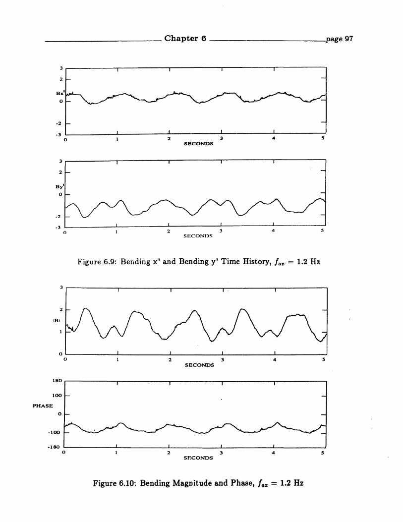
____________ Chapter 6 page 97
3
2
0
-2
-30 2 3 4
SECONDS
3
2
By'
0
-2
-3() 2 3 4 5
SECONDS
Figure 6.9: Bending x' and Bending y' Time History, fez = 1.2 Hz
3r-------"""r"-------......------_-----~-----.......,
2
IBI

__---------- Chapter 6 , page 98
3fax=6.0 Hz. [s=200 Hz. T=l sec.------------
2
Byo 0)
-2
32oRx'
-2
.3 """'--__"'-- ....... ..a..-_-----'
-3
Figure 6.11: Bending x' versus Bending y', foz = 6.0 Hz
2r------..------~------,--------------
Ox'
o
-1
0.80.60.40.2
-2 ..L..-- .....L..- ...L- -L- -J
oSECONDS
2 .-'-----~-----~------,--------...-------
1
By'
o
-1
0.80.60.40.2
-2 """----------11...-- --.a.. --"-__--_-.L --J
oSECONDS
Figure 6.12: Bending x' and Bending y' Time History, IClz = 6.0 Hz

_------------ Chapter 6 page 99
2 _--------------r------,-------.,..--------,
1.,5
lnl
Figure 6.13: Bending Magnitude and Phase! foz = 6.0 Hz
., fax=7.! Hz. f5=200 Hz. T=l sec..' r---.-----~-~--.:...-:......----......---
2
By'
o
-2
32oOx'
-2
-3 oA-... ....... .......__.....
-3
Figure 6.14: Bending x' versus Bending y't laz = 7.1 Hz

_____________ Chapter 6 ----- page 100
2------~------.....--------.-----------------
o
-1
-2o 2
SECONDS3 s
2_-----..........------.......---------r-------r--------.
-2o
SE(~()NI')S
3 4
Figure 6.15: Bending x' and Bending y" Time History, la,; - 7.1 Hz
2r-------..........------........-----.......,.-------r--------,1..5
181
o.s
SECONDS
6000
4000
PHASE
2000
-2000 2 3 4
SECONDS
Figure 6.16: Bending Magnitude and Phase, foz = 7.1 Hz

r fax=12.6Hz. (5=200 Hz, T=1 sec.:' r-----'T----r----~~-- ---__
By'
o
4 52
Radial
oBx'
-2
-4
-5 ~---" --'- __L .....L_____'
-5 -4
Figure 6.17: Bending x' versus Bending y', 10% = 12.6 Hz
SECONDS
Figure 6.18: Bending x' and Bending y' Time History, /o,z = 12.6 Hz
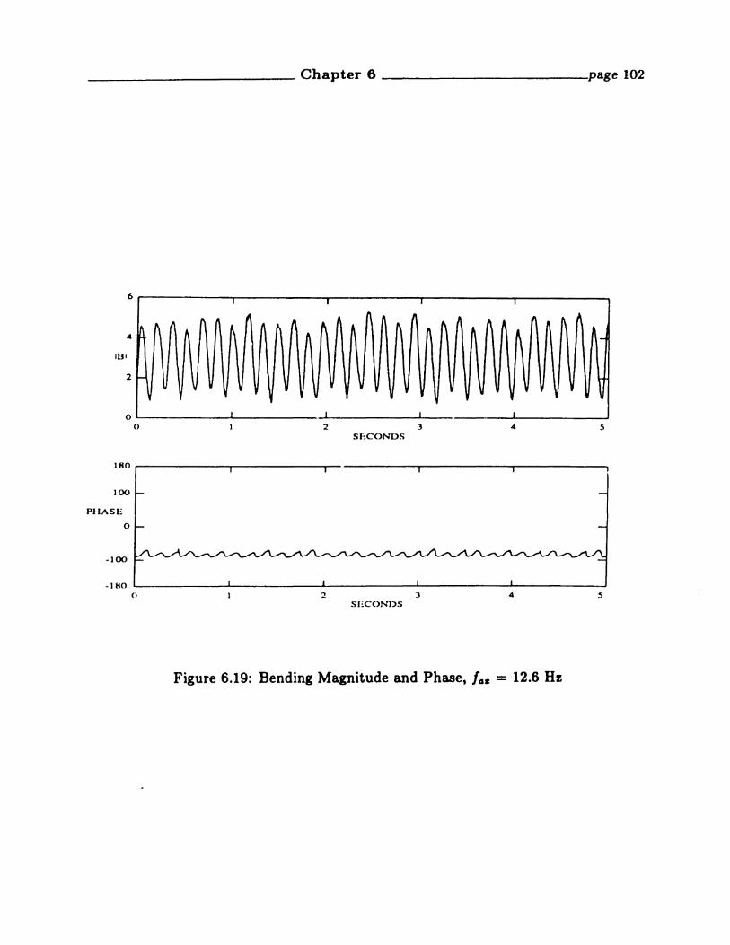
______------- Chapter 6 page 102
6,--------,.--------r--------.,.------_-----_
4
o --'- ....... ...L.__. -'-- --J
0235 ECOl'wnS
ISO r---------.----------..------~-----__.._-----_
432
o
100
-100
-180 '-- ......... ~ ____. -&- ____J
()
PIIASE
SI:'C(>NI)S
Figure 6.19: Bending Magnitude and Phase, fOE = 12.6 Hz

Chapter 7
Field Tests
A series of downhole vibration tests were conducted in Quitman, Texas, in Au
gust of 1984. This experiment was a joint effort of Shell Development Co. and NL
Industries. The purpose of the test was to record the BHA vibration near the bit.
The data from this experiment were made available to this research project.
7.1 Background
The downhole sensors package of this experiment included the transducers for
WOB, TOB, two perpendicular bending measurements, and three axes of acceleration
measurements. The sensor package has been described in (52]. A sketch of the sensor
package is shown in Figure 7.1 . The signals from the sensors were first sampled by an
AID systeID, then, the data were transmitted to the surface by a hardwired telemetry
system. For the results presented here five sensors were sampled in a given test at 130
Hz per channel. The channels to be sampled were selected by the control system at
the surface. A total of 60 hours of data were taken during this experiment. Following
is a summary of the experimerit
• Bit type used : Tri-cone and PDC bits
• Footage drilled : 4000' to 7000' in a vertical well through shale, limestone, and
sandstone
103

_____________ Chapter '1 page 104
Sensor package (top view)
axial acc.
tangential ace.
radial ace.
Bx'
Figure 7.1: Top View of the Sensor Package
• RPM : 50 to 200
This set of data is unique because of the high data rate provided by the hardwired
telemetry system.
7.2 Data Processing
The accelerometers used were not suitable for making low frequency measurement,
such as experienced in forward synchronous whirl. Furthermore, the acce)erome~ers
are much more sensitive to wall impact than strain gages. For these reasons, the
bending moment data are emphasized in the results shown below which specifically
emphasize whirling behavior.
From the raw time histories, we have learned that the measurements are often
very random in nature, seldom remaining stationary for a long period of time. In
order to resolve the spectral peaks, the Maximum Entropy Method (MEM) was used

exclusively to estimate the spectral results. This method is known for its ability to
give high resolution estirr!ates of the spectrum from relatively short records, making
it suitable for processing these datar
7.3 Case Studies of the Bending Vibration andWhirling Motion
Due to a lack of adequate downhole vibration data, very little has been known
about the actual bending dynamics experienced by the drill string while rotary drilling,
and about the contributions of bending vibration to drill string deterioration and
failure. "Recently, downhole vibration recorders and systems with hardwires to the
surface have provided much needed data and insight into events downhole. At first
glance, the data appears, even to the experienced vibration analyst, extremely com
plex. Many different vibration phenomena occur simultaneously, making it difficult
to isolate, evaluate, and explain anyone of them. To varying degrees, axial, torsional
and bending vibration are all present and at times intimately coupled. Bit bounce,
stick slip, forward and backward whirl, and linear and parametric coupling between
axial and bending vibration all occur.
Several authors have made recent contributions to the measurement of bending
" vibration of BHA'5. Wolf et aI, [52), present samples of downhole vibration data
acquired in the same well as the data presented here. Included in tile paper are
several suspected cases of whirling. The paper by Besaisow et aI, (6], also shows
suspected examples of bending vibration and whirling. Burgess, et aI, (9J, specifically
conclude that transverse vibration is a source of downhole MWD tool failure, and
cite a method for reducing downhole failures. Close et ai, [13], present downhole
recordings of large amplitude bending vibration.

l
ITA.ll'ZIR
..,....-- RU••,NO
.IT
Figure 7.2: Whirling Drill Collar
7.3.1 Bending Moment Measurements
Bending moments are deterI!lined by the curvature of the drill collar. Referring to
Figure 7.2, let the deflection of the collar center as a function of z, the axial coordinate,
be designated by Vo (z, t). As an approximation to the actual deflection assume that
the whirl deflected shape of the drill collar is the half sine wave given by:
tJo(z,t) = (& - Rc)ain(7rz/L)F(t) (7.1)
where L is the length of the drill collar section from the bit to the stabilizer and F(t)
is an arbitrary function of time. Thus, in this instance, Figure 7.3 depicts a croes
section at the midspan of the drill collar. The bending moment corresponding to
tlo(z, t) is given by the moment-curvature relationship
B(z, t) = El~:; = -(& - Rc)(El1t2/ L2)sin(7rz/L)F(t) (7.2)
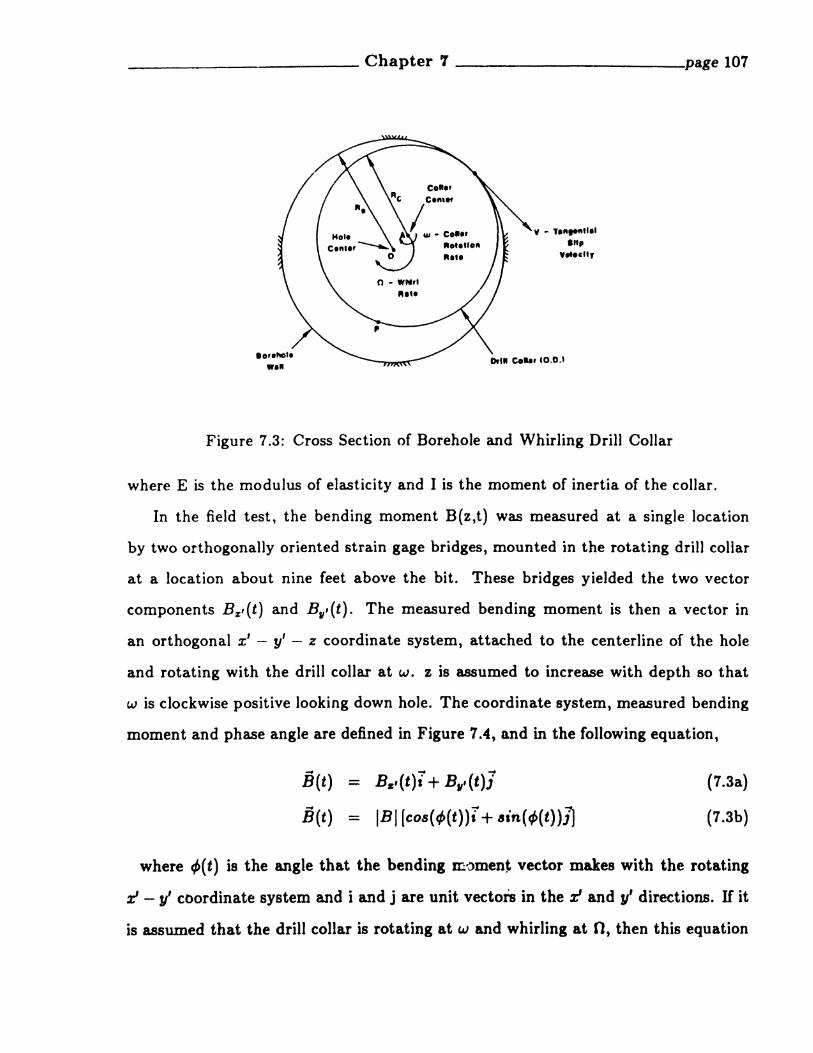
loreMI..."
y - ,a......tlllIn,
v"'clt,
Ort. c..., CO.OJ
Figure 7.3: Cross Section of Borehole and Whirling Drill Collar
where E is the modulus of elasticity and I is the moment of inertia of the collar.
In the field test, the bending moment B(z,t) was measured at a single location
by two orthogonally oriented strain gage bridges, mounted in the rotating drill collar
at a location about nine feet above the bit. These bridges yielded the two vector
components Bz,(t) and BII,(t). The measured bending moment is then a vector in
an orthogonal x' - y' - z coordinate system, attached to the centerline of the hole
and rotating with the drill collar at w. z is assumed to increase with depth 80 that
w is clockwise positive looking down hole. The coordinate system, measured bending
moment and phase angle are defined in Figure 7.4, and in the following equation,
B(t) - Bz/(t)i+ BII/(t)J
B(t) - IBI [COS (<f>(t)) i + "in(<f>(t)).1l
(7.3a)
(7.3b)
where <p(t) is the angle that the bending momen~ vector makes with the rotating
~ - y' coordinate system and i and j are unit vectors in the ~ and 1/' directions. IT it
is assumed that the drill collar is rotating at w and whirling at 0, then this equation

_____________ Chapter 7 ----------__page 108
yl
Dri11 CoIIar
Borehole
o :Center of the Borehole
Figure 7.4: Coordinate System, Bending Moment, and Phase Angle Definition
may be expressed as shown below:
B(t) = IBllcos((w - O)t)i+ sin((w - O)t)Jj (7.4)
The rotating x' - y' coordinate system representation is particularly useful, because
it represents the bending moment time history that is experienced by the collar and
is therefore a measure of the stress time history which is relevant to cyclic fatigue
damage. An important feature of this expression is that the bending moment, and
hence t~e bending stresses, vary as the difference between the drill collar rotation
rate, w, and the whirl rate, o. The difference frequency is the frequency of stress
cycles which would be experienced by the drill collar under whirling conditions.
Equation 7.4 is valid for all whirling conditions, whether or not in contact with
the wall. One must only evaluate the magnitude and correct sign (plus for clockwise
rotation and minus for counter-clockwise rotation) of the drill collar rotation and
whirl rates. The unwrapped phase angle, ,p(t) can be estimated from B~,(t) and

__, Chapter 'I -------- page 109
lJu,(t), the independently measured bending moment components, 8.8 follows, where
cl>o is a constant depending on initial conditions.
4>(t)
tP(t) - arctan [B.,t (t)/Be,(t)] + tPo
arctan(sin((w - O)t)/cos((w - n)t)] + tPo
- (Cot] - O)t + tPo
~~ = (w - 0)
(7.Sa)
(7.5b)
(7.Sc)
Therefore, from two independent and orthogonal bending moment measurements
the difference between the whirl rate and drill collar rotation rate can be determined.
In the case studies, plots of q,(t) will often be presented. The slope of these plots is
the phase rate, 4>, which from equation 7.Sc for whirling, is the difference frequency
(w - 0). Since the rotation rate w is usually known from surface observation, then
the whirl rate n can be deduced. The term 'unwrapped' phase angle refers to the way
the arctan function is computed from real data. The arctan function used here is not
restricted to a range of -7r to +1T. Rather, the phase angle is meant to accumulate
linearly with time as shown in equation 7.5b.
Linear coupling between axial force and lateral deflection also produces time vary
ing changes in bending moment. Unfortunately, because whirling produces curvature,
and curvature is needed for linear coupling to occur, then the two phenomena are likely
to occur together. As a result, bending moment measurements would contain compo
nents due to the whirling at the difference frequency ((A.1 - 0) and also components due
to the linear coupling to the axial force at the bit, which for the purpose of discussion
is assumed to be at a frequency Wa • When both sources of vibration are present to
a significant degree in the measuremerlt, then attempts to use the unwrapped phase
t/>(t) from equation 7.5a may be impossible. However, computation of the autospectra
of either the x or y components of the bending moment should reveal strong peaks at
both (w - n) and W O •
As disc~ above, the various bending vibration mechanisms do not generally

occur one at a time, but in fact many phenomena may occur simultaneously. As a
cons~quence, the bending moment and phase angle time histories are rarely as simple
as those shown in equations 7.5b and 7.5c. They are usually much more complex. On
occasion, singie ph€nomena do dom~nate. The case studies shown below have been
carefully selected to separately reveal dominant examples of each mechanism.
7.3.2 Drilling Case Studies
In this section, examples of dr~11 collar whirling, linear eoupling of axial and bend
ing vibrations, and parametric excited bending vibration are presented. All cases
described here were for pendulum BHA '8. In Cases 1, 2 , 3 , and 6, the sensor pack
age was placed just above the bit, with 59.8 feet separating the bit and the center of
the first stabilizer, and 35.2 feet between the centers of the first and second stabilizers.
The drill collar between the first and second stabilizer was 6.25 inches, outside diam
eter. The remainder of the BHA was typically composed of 19 to 23, 6.25 inch drill
collars above the second stabilizer. In Cases 4 and 5, the sensors are placed just above
the second stabilizer. The length from the bit to the middle of the first stabilizer was
approximately 65 feet, and from the first to the second stabilizer, 35 feet.
Six case studies are presented here, carefully chosen to illustrate the variety of
pherlomena described in previous chapters. Considerable use is made of the bend
ing moment measurements, Bz,(t) and BI/,(t), and the bending moment phase angle
4>(t), which is useful in determining the type of whirl and the whirl rate. For the
Quitman experiment, RPM was not electronically recorded. For some tests downhole
magnetometer data was available, from which RPM can be deduced. For the six
cases presented here, which best represent the phenomena under study, magnetome
ter data were not available. Occasional surface logbook entries were the only record
of RPM. This handicap was overcome by extracting the information from the other
measurements, for ~xample, dynamic WOB.

____________ Chapter 'I page III
7.3.3 Case l.: No Whirl And SilIlple Rotation of a CurvedDrill Collar.
Figure 7.5 shows a two second time history for the Qending moment components
B z ' and Btl I and Figure 7.6 shows q'.>(t), the unwrapped phase angle. The data was
acquired while drilling with a PDe bit through shale at an average rate of penetration
of 11 ft/hr at depth of approximately 6846 feet. There were 16 drill collars, jars, and
5 more drill collars above the second stabilizer. From only the bending moment time
series, it is impossible to deduce the behavior of tIle drill collar. The plot of th~
time history of the phase angle <p(t) reveals a mean phase rate or slope of about 500
degrees/sec., which is equal to approximately 1.4 Hz (84 RPM). This is confirmed by
computing the spectrum of Bz(t), as shown in Figure 7.7, which has its highest peak
at 1.36 Hz. If it is assumed that there was no whirl, then from equation 7.4 with n set
equal to zero, we conclude that the rotary speed w was 1.36 Hz (81.6 RPM). For this
data set, there was no magnetometer recording of RPM. However, a manual record
kept in a surface logbook indicated that the surface rotation rate was approximately
80 RPM.
~t is interpreted that the drill collar was bent, probably rubbing against the wall,
but not whirling. The strain gages were exposed to a bending moment of approxi
. mately 10000 ft-lb peak to peak. Some additional bending vibration was superimposed
on top of that due to the curvature and rotation. This vibration was probably caused
by coupling with bit forces or bumping agai!lst the wall.
7.3.4 Case 2: Forvvard Synchronous Whirl w = n
Figure 7.8 shows the time histories for the bending moments and Figure 7.9 ShOW6
the unwrapped phase angle. The data was acquired while drilling through shale with
a PDC bit at. an average rate of penetration of 60 ft/h:t at depth of 4366 feet. 'l'he
rotary speed, manually logged at the surface, was 116 RPM. There were 23, 6.25 inch
drill collars above the second stabilizer. The time history for the phase angle, shown

21.51SECONDS
O.S
ooסס1 _--------.--------~-------r----------,
OOסס1- L- -I--------"'---------'----------'o
5000
Bx'CFT-LB)
o
ooסס1
·sooo
OOסס1- l..- --L-------L-------..-L---------""o u.S J J.5 2
SECONDS
Figure 7.5: Time History of the Bending Moments for Case 1: No Whirl, Pure Rotation
1000 __------~---------T-------~------.....,
DEGREES
500
o
..100 L..._------1..-------l-------.L.--------o 0.5 1 1.5 2
SECONDS
Figure 7.6: Time History of Unwrapped Phase Angle for Case 1: No Whirl, PureRotation

in Figure 7.9, reveals that the mean phase angle remained constant. Vibration, not
whirling, is revealed as additional fluctuations in phase angle about the mean. Figure
7.10 shows the bending moment spectra, which reveal peaks at 1.85 HZ.(111 RPM),
which is close to the reported rotation rate of 116 iiPM.
The int~rpretationfor this case is that the zero average phase rate indicates that
the drill collar was exhibiting forward synchronous whirl. The peak in the bendin~
moment spectra at 1.85 HZ.(111 RPM) indicates that some additional rotation rate
vibration was also occurring. This vibration was probably caused by the collar hitting
the wall once per rotation. However, any cause which would result in a once per
revolution perturbation in the circular whirl orbit would have the same result.
7.3.5 Case 3: Backward Whirl With Little Slip
Figure 7.11 shows the time history for the bending moments and Figure 7.12 shows
the phase angle. The data was acquired while drilling through limestone with a tri
cone bit at an average rate of penetration of 18 ft/hr at depth 5259 feet. The BHA

____________ Chapter '1 page 114
.5000 _-------.,.----------,r--------,.----------,
2.500
Bxtf-i-LB)
o
-2S00
.. 5000 1-_------L---------Il....-------~-------2~o o.s 1 1.5
SECONDS
SOOO _------~--------,r-------..,.----------,
2500
BytFT-LB)
o
-2500
.. 5OCX) L-__-----L---------JL...-------~-------~2o 0.5 I 1.5
SECONDS
Figure 7.8: Time History of Bending Moments for Case 2: Forward SynchronousWhirl
1000 _-------r------,--------,------i
500
DEGREES
o
-500
-1000 L_----.L.-----....1------~-----_:_'2o 0.5 1 ~!.s
SECONDS
Figure 7.9: Time History of Phase Angle for Case 2: Forward Synchronous Whirl

was a pendulum assembly with 20 drill collars, jars and 9 heavy weight drill pipe
above the second stabilizer. The bending mon!ent time series reveal peak to peak
amplitudes of about 25,000 ft-lbs, which is several times greater than seen in the two
previous examples. Figure 7.12 reveals an excellent example of the phase angle t/J(t)
during backward wllirI. The mean phase rate or slope of the plot is a constant 1900
deg./sec., which equates to 5.28 Hz. The spectra for Bz ' and B fI , shown in Figure 7.13
also reveal strong peaks at 5.28 Hz.
IT the assumption is made that this is a case of backward whirl with no slip, then
equation 5.2 would predict that O. = -4w, and the difference frequency or phase rate
predicted by equation 7.Sc would be at five times the rotation rate, as shown in the
following expression:
(0, - w)/21r = -Sw/21r = 5.28Hz
From this, the conclusion is reached that the rotation rate w/21f was 1.06 Hz (63
RPM). For this case, the surface speed was reported in the logbook as 80 RPM.
The explanation for the discrepancy between the reported rotary speed of 80 RPM

and the calculated drill collar rotation rate of 63 RPM is not certain. One possibility
is a reporting error, because the RPM was only occasionally written down. However t
a more likely explanation is that the collar was slipping some as it whirled. H it is
required that the rotation rate be as recorded, w /21f = 1.33 Hz (80 RPM), then it is
concluded from Equation 7.Sc that
(w - n}/21r = 5.28Hz
n/21r = -3.95Hz
as opposed to
nb /21r = 4w /21r = -S.32Hz
which would be expected under no slip conditions. From equation 5.2, the whirl
ratio, s, is concluded to be 0.74. In the absence of an accurate determination of
surface rotation rate, it is concluded that this is an example of backward whirl with
some slip, although it is possible that there was no slip. Figure 7.14 is plot of Bz,(t)
versus BII,(t) for this example. Each of the four images presents 0.5 seconds of the
total 2.0 seconds of bending moment data. In the absence of superimposed vibration,
the whirling would be expected to produce orbits in a plots such as these with a
frequency equal to the phase rate of 5.28 Hz. These plots make it clear that even
though whirling is the dominant phenomenon in this example, there is substantial
additional motion of the drill collar due to other sources of vibration.
'1.3.6 Case 4: Backward Whirl With Substantial Slip
Figure 7.15 shows the time history for the bending moments and Figure 7.16 shows
the phase angle. The data was recorded while drilling with a tri-cone insert bit, in
shale, at a depth of 6897 feet. The reported rotary speed was 60 RPM (1.0 Hz). The
BHA was a pendulum assembly, as described earlier, with the NBMS, followed by
fourteen, 6.25 inches collars between the second stabilizer and the jars and five drill
collars above the jars. The reported measurements thus came from a point a few feet

20000 -------~------........,.-------r------____,
10000
Bx~-LB)
o
-10000
-20000 l- ..l- --l ..&..- _
o 0.3 1 loS 2SECONDS
20000 -------....,..--------,-------,-------.,
10000
By'CFf-LB)
o
-10000
-20000 L..-------L---------1-------""""--------~2() 0.5 J J.S
SECONDS
Figure 7.11: Time History of Bending Moments for Case 3: Backward Whirl withLittle Slip,s = .75
4000 -------.---------r-------r------j
3000
DEGREES
2000
1000
0.5 1SECONDS
1.5 2
Figure 7.12: Time History of Phase Angle for Case 3: Backward Whirl with LittleSlip, s = .75

20000 ...- 0_.....0 ~S......F..c.....O....."'....)_----,
.. IOCJ()() •••••••••••••
By(FT·LB)0·· ....~.~----...o"lI
-20000 L-.. ~
-20000 0 20000Ba(FT-LB)
.2XJOO '----------'..20000 0 20000
RI(PT·I..R)
By(FT·LI)o .
ooסס1· "/" .
·20000 ..20000 0 20000Ra(FT-I ..R)
Figure 7.14: Orbital Plots of Bending Moments for Case 3: Backward Whirl withLittle Slip, s = .75

14000 ---------,----
7000
Bx'(FT-LB)
o
-7000
-1.t000 L-------L-------I--..------L.------~2o O.S 1 1.S
SECONDS
14000 -------.--------..-------r--------;;,
-7000
-14000 L---------.JL---------Jl..-----------IL.---------=-2o 0.5 I 1.5
SECON1)S
Figure 7.15: Time History of Bending Moments for Case 4: Backward Whirl withSubstantial Slip, S = .58
above the second stabilizer.
Figure 7.16 shows that the mean phase rate was 1200 degrees/sec (3.33 Hz). Thus,
the difference frequency, (w - n)/21r, was 3.33 Hz. This is verified by the location
of the peaks of the bending moment spectra, shown in Figure 7.17. Requiring w/21r
to be 1.0 Hz. results in an estimate for O/21r of -2.33 Hz. Using Equation 5.2, the
backward whirl rate without slip is predicted to be Of> = -4w = -4.0 Hz. The actual
backward whirl rate is about half that expected with no slip, and the whirl ratio
computed from equation 5.3 is, therefore, s = 0.58. The drill collar was backward
whirling and slipping at the same time.
Even with the admitted uncertainty in the recorded RPM, it is extremely unlikely
that the surface RPM was less than 60. If the surface RPM was greater than 60 RPM
reported, then calculations similar to the ones conducted above would reveal that the
drill collar was backward whirling and slipping even more.

------------ Chapter 7' ----------__page 120
3000 --------....,....--------,---------..,r----------,
2000
DEGREES
1000
o
21.5
J-500 L.- -L- . __
o 0.5 1SECONDS
Figure 7.16: Time History of Phase Angle for Case 4: Backward Whirl with Substantial Slip, s = .58
30
30
25
25
20
20
ISHz
15Hz
10
10
s
...: Se+06::E~. 4e....06Vi'=-oJ
~ 3e+06
[ 2e+06
...'"M'le+06=
00
~5e+06
• ~+06
~-Tl; 3e+06
I 2e+06
_V)
~ le+06
00
Figure 7.17: Bending Moment Spectra for Case 4: Backward Whirl with SubstantialSlip, s = .58

____-------- Chapter '1 page 121
7.3.7 Case 5: Linear Coupling of Axial and Transverse Vibrations
Figure 7.18 shows the time histories of weight on bit and one component of bend
ing, Bz,(t), while drilling through shale with a tri-cone bit at an average rate of
penetration of 7 ft/hr. The depth was 6899 feet, and the approximate reported rota
tion rate was 60 RPM. The BHA the same as in case 4 above, with the measurements
originating from a point just above the second stabilizer. This is a classic case of
bit bounce, as can be seen by the large variation in WOB (45000 pounds peak to
peak) and the flat bottoms at zero weight on bit when the bit leaves the bottom. In
this figure, compression is positive. At first glance, the bending moment time series
appears to contain little useful information.
Figure 7.19 shows the autospectra of the WOB and B z' time series. Both spectra
show dominant peaks at the same frequency of 2.9 Hz. In this case, 2.9 Hz is the
three times RPM cone rate which would result from a rotation rate of 0.97 Hz (58
RPM). This is consistent with the reported rotation rate of 60 RPM. In the WOB
spectrum, the 6 times RPM higher harmonic is also evident. The reason that multiples
of the 3 times RPM cone rate exist is that cone rate excitation is a periodic but not
sinusoidal process. Therefore, higher order components at 6, 9, and even 12 times
RPM frequently occur in axial and torsional vibration measurements, because they are
necessary terms in the Fourier series, which make up the periodic, but non-sinusoidal,
shape of the time series.
In this example, bit bounce occurs because of probable coincidence of strong 3
times RPM axial excitation and a longitudinal resonance of the drill string. The fact
that both the WOB and Bz' spectra have dominant peaks at the same frequency is a
significant initial indication of linear coupling. Further evidence can be acquired by
computing the cross spectrum and the coherence between Be' and WOD. Figure 7.20
shows the phase portion of the cross spectrum and the coherence. The coherence is a
measure of the degree to which a linear cause and effect relationship can be established
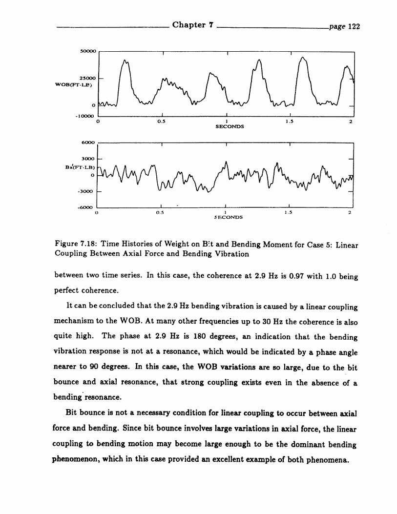
2.5000
WOB(FT-LP)
0
OOסס1-
0 0.5 1 I.S 2SECONDS
6000
3000
Bx'crr·LB)
0
-3000
-6000() 0,5 1 1.S 2
5' ECONDS
SOOOO -------_------......,.---------y---------,
Figure 7.18: Time Histories of Weight on B~.t and Bending Moment for Case 5: LinearCoupling Between Axial Force and Bending Vibration
between two time series. In this case, the coherence at 2.9 Hz is 0.97 with 1.0 being
perfect coherence.
It can be concluded that the 2.9 Hz bending vibration is caused by a linear coupling
mechanism to the WOB. At many other frequencies up to 30 Hz the coherence is also
quite high. The phase at 2.9 Hz is 180 degrees, an indication that the bending
vibration response is not at a resonance, which would be indicated by a phase angle
nearer to 90 degrees. In this case, the WOB variations are so large, due to the bit
bounce and axial resonance, that strong coupling exists even in the absence of a
bending· resonance.
Bit bounce is not a necessary condition for linear coupling to occur between axial
force and bending. Since bit bounce involves large variations in axial force, the linear
coupling to bending motion may become large enough to be the dominant bending
phenomenon, which in this case provided an excellent example of both phenomena.
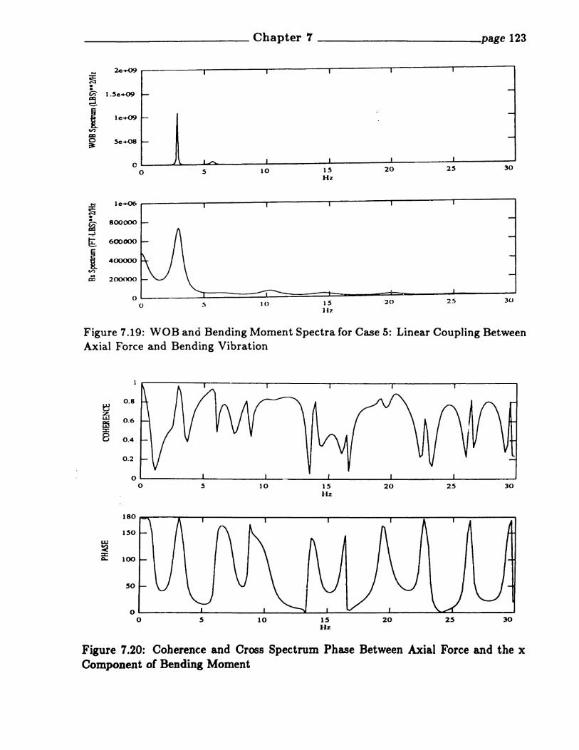
Chapter '1 page 123
2Cl+09 IN I 1 I I
~·· -Vi" I.Se+09 ~
~
d.
I le+09--
U')
= -0 Sc+08 -it;
Jl 1J""t".. I I I IC
20 2S 300 S 10 15
Hz
N le+06
~· 800000~...,J
~ 600000
I ooסס40
(,;II")
IlC2CXXlOOcc
020 25 30
0 5 }O 15lIz
Figure 7.19: WOB and Bending Moment Spectra for Case 5: Linear Coupling BetweenAxial Force and Bending Vibration
Figure 7.20: Coherence and Cross Spectrum Phase Between Axial Force and the xComponent of Bending Moment
____________ Chapter 7' page 124
703.8 Case 6: Parametric Excited Bending Vibration
The mechanism for the pa.rametric excited bending vibration is described in chap
ter 4. This phenomenon involves a quadratic relationship between WOB(input) and
bending(output). To verify this phenomenon, a large number of data points are
needed for the signal processing FFT algorithm. From the experience in evaluating,
the BHA bending vibration seldom remained stationTJJ'Y for more than 10 seconds.
Therefore, a special signal processing technique was developed to extract parametric
excited bending vibration form a record length of only several seconds. The method
is described below. Assuming that x(t) is the input and y(t) is the output, to a
quadratic system, the input-output relationship is x = y2, The following steps may
be used to verify the quadratic relationship between input and output:
1. square the time history of x(t)
2. compute the linear coherence between the squared time history of x(t) and the
y(t) time history using the two channel Maximum Entropy spectral analysis
method
The coherence function thus obtain is termed quadratic coherence. The quadratic
relationship between input and output is revealed as the peaks in the quadratic co
herence. For example, if a peak of quadratic coherence is at 4 Hz, this indicates that
the 4 Hz component in II resulted from squaring the 2 Hz component in x. Now we
proceed to the example from the Shell data.
The example is drawn from data taken at 5138 feet, using a Hughes J22 tri-cone
bit. The RPM is deduced from the WOB spectruin, which is shown in Figure 7.21.
The principal peak is approximately 3 Hz. This peak usually corresponds to three
times RPM generated by the cone passage. Thus, we can infer infer that the rotation
was ~bout 60 RPM.
Figure 7.22 shows the bending moment spectra measurements in two perpendicular
planes. They reveal principal peaks at 1.5 Hz, half of the peak frequency from the

_____________ Chapter '1 - page 125
le+09 ----------,1----------'1------------,
8e+08 -'--N
~••tf)c:-J 6e+08 .....-Eg~
ent:C
4e+08 -0 -~
2e+08 ~-
oL_.LJ-~~~-__..LI--------""'--I--------o 10 20 30
Hz
Figure 7.21: WOB Spectrum for Case 6
WOB spectrum.
A test for linear coupling was performed by computing the linear coherence be
tween B z' and the WOB time history. The upper trace of Figure 7.23 is the linear
coherence, which reveals a coherence of 0.65 for both peaks at 1.5 Hz and 3 Hz. This
indicates that some bending vibration was resulting from linear coupling mechanisms
with WOB dynamic fluctuations. The lower trace of Figure 7.23 is a quadratic co
herence plot. It reveals a coherence of 0.75 at 3 Hf" which is twice the frequency of
the bending peak and corresponds to the WOB dOUlhiaJi~ peak. This is an ;"~xample
of parametric excited bending vibration of the BHA•.

e 0.8
~ffi 0.6::c8~ 0.4
~0.2..oJ
5 10 IS 20 2SHz
ei; 0.8
0 0.6=8U 0.4~ccc 0.2-<:::»0'
Figure 7.23: Linear and Quadratic Coherence Between WOB and Bending x for Case6
Chapter 8
Conclusions and Suggestions
The goal of this thesis was to provide insights into the bending vibration of Bottom
Hole Assemblies. Unlike axial and torsional vibrations, bending vibrations generated
at the bottom are not transmitted to the surface through the drill string. Though, it
may be possible to see the evidence of downhole bending vibration in in the surface
axial and torsional vibration signals, the relationships are not well enough understood
to be used diagnostically.
We started out by examing the mechanisms that cause the bending vibration in
the BHA. These mechanisms are described in Chapters 3, 4, and 5. The laboratory
tests revealed the important properties of linear and parametric coupling between
axial and bending vibration. The tests also showed that the excitation frequency
needed to drive the shaft at resonance for either type of coupling, varies linearly with
respect to rotational frequenoy of the shaft.
Evidence of these two types of coupling were also found in the the data acquired
during a field test. This data set also provides examples of the whirling behavior.
Forward synchronous whirl and backward whirl with slip have been found in this
data set. Forward whirl can cause abrasive wear of the drill collar outside diameter,
and is a probable c&'use of flat spots. Backward whirl usually associated with high
bending moments and high bending cycles. Therefore, it can shorten the fatigue life
of drill collars and tool joints.
This research indicates that further work needs to be done in
127
~~~~~~~~~__~~Chapter8~~~~~~~~~~~~p~e128
1. predicting the onset of backward whirling
2. verifying the existence of parametrically excited bending vibration in cases of
extensive wall contact as would be experienced in slick aasemblies or above all
stabilizers.
3. investigating the influence of bending dynamics on directional drilling

Bibliography
[1] T. D. Aarrestad, H. A. Tenne~en, and A. Kyllingstad. "Drill String Vibrations:
Comparison Between Theory and Experiments on a Full-Scale Research Drilling
Rig". In Proceedings ofIADC/SPE Conference, February 1986.
[2] J. A. Baird and M. C. Apostal. "An2 ·Jzing the Dynamic Behavior of Some Typi
cal Rotary Bottom Hole Assemblies During Startup". Transaction 01 Geothermal
Resources Council, 9:83-89, August 1985.
[3] J. A. Baird and B. C. Caskey. "Analyzing the Dynamic Behavior of Down
hole Equipment During Drilling". Trar..saction 01 Geothermal Resources Council,
8:243-247, August 1984.
[4] J. A. Baird and et. ale "GEODYN2: A Bottom Hole Assembly-Geological Forma
tion Dynamic Interaction Computer Program". SPE Conference Paper Number
1~ge8, September 1985.
[5] A.' A. Besaisow, Y. M. Jan, and F. J. Schuh. "Development of a Surface Drill
string Vibration Measurement System". SPE Con/erenee Paper Number 14Se7,
September 1985.
[6] A. A. Besaisow and M. L. Payne. "A Study of Excitation Mechanisms and
Resonances IndllCing BHA Vibrations". SPE Conference Paper Number 15560,
October 1986.
[7J R. D. Blevins. Formulas lor Natural Frequency and Mode shape. Van Nostrand
Reinhold Co., New York, New York, 1979.
129

BIBLIOGRAPHY 130
[8] M. J. Briggs. Multichannel Maximum EntroPJI Method of Spectral AnalJlsis Ap
plied to Offshore Struetures. Ocean Engineer thesis, Massachusetts Institute of
Technology, 1981.
[9] T. M. Burgess, G. L. McDaniel, and P. K. Das. "Improving BHA Tool Relia
bility with Drillstring Vibration Models: Field Experience and Limitations". In
Proceedings 0/1987 IADC/SPE Conference, New Orleans, March 1987.
(10] R. B. Campbell. The Estimation 01 Natural Frequenc" and Damping Ratio 01
Offshore Structures. PhD thesis, Massachusetts Institute of Technology, 1980.
[11) S. S. Chen, M. W. Wambsganss, and J. A. Jendrzejczyk. "Added Mass and
Damping of a Vibrating Rod in COl1fined Viscous Fluids". Journal 0/ Applied
Mechanies, 326--329, June 1976.
[12] Wilson C. Chin. "Fatal Tubular Bending Motions Difficult to Detect Uphole".
Offshore, 32-36, April 1988.
[13] D. A. Close, S. C. Owens, and J. D. MacPherson. "Measurement of BHA Vi
bration Using MWD". In Proceedings 0/ 1988 IADC/SPE Conference, Dallas,
March 1988.
[14] S. H. Crandall. "The Physical Nature of Rotor Instability Mechanisms". In
Rotor Dynamical Instability, June 1983.
[15] R. A. Cunningham. "Analysis of Downhole Measurement of Drill String Forces
and Motions". Transaction of ASME, 208-216, May 1968.
[16] D. W. Dareing. "Drill Collar Length is a Major Factor in Vibration Control".
Journal 01 Soeiety 01 Petroleum Engineers, 637-644, April 1984.
[17] "F. H. Deily and et. al. "Downhole Measurement of Drill String Forces and Mo
tions". Journal 01 Engineering lor Industrfl, 217-225, May 1968.

BIBLIOGRAPHY 131
[I8} S. M. Dickinson. "The Lateral Vibration of Slightly Bent Slender Beams Sub
ject to Prescribed Axial End Displacement". Journal 01 Sound and Vibration,
68(4):507-514, 1980.
[19] V. A. Dunayevsky, A. Judzis, and W. H. Mills. "Dynamic Stability of Drill
strings Under Fluctuating Weight-on-Bit". SPE Conference Paper Number
l.1Se9, September 1985.
[20] V. A. Dunayevsky, A. Judzis, and W. H. Mills. "Onset of Drillstring Precession
in a Directional Borehole". SPE Conference Paper Number 190e7, September
1984.
(21] F. B. Hilldebrand. Advanced Calculus lor Applications. Prentice-Hall, Engle
wood Cliffs, New Jersey, 1976.
[22] C. S. Hsu. "Further Results on Parametric Excitation of a Dynamic System".
Journal of Applied Mechanics, 373-377, June 1965.
(23] C. S. Hsu. "On the Parametric Excitation of a Dynamic System Having Multiple
Degrees of Freedom". Journal 01 Applied Mechanics, 367-372, September 1963.
[24] T. Iwatsubo and M. Saigo. "Parametric Instability of Clamped-Clamped and
Clamped- Simply Supported Columns Under Periodic Axial Force". JDurnal 01
Sound and Vibration, 30(1):65-77, 1973.
[25] T. Iwatsubo, Y. Sugiyama, and S. Ogino. "Simple and Combination Resonances
of Columns Under Periodic· Axial Loads". -Journal 01 Sound and Vibration,
33(1):211-221, 1974.
[26] G. M. Jenkins and D. G. Watts. Spectral Anal"s"s and its Applications. Holden
-Day, 1968.
[27] N. R. Joglekar. Ezperimental Evaluation 01 Rotor Motion With Radial Rub.
Master's thesis, Massachusetts Institute of Technology, June 1987.
BIBLIOGRAPHY 132
[28] J. Y. Jong. The Quadratic Correlation Between In-Line and Cross-Flow Vortex
Induced Vibration 0/ Long Flexible CJllinderB. PhD thesis, Massachusetts Insti
tute of Technology, 1984.
[29] John L. Kennedy. Fundamental, 0/ Drilling. PennWell Publishing Company,
Tulsa, Oklahoma, 1983.
[30] C. S. Kim and S. M. Dickinson. "The Flexure Vibration of Slightly Curved Slen
der Beams Subject to Axial End Displacement". Journal 0/ Sound and Vibration,
104(1):170-175,1986.
[31] Y. C. Kim. Nonlinear Vibration 0/ Long Slender Beams. PhD thesis, Mas
bachusetts Institute of Technology, 1983.
[32] Y. C. Kim and E. J. Powers. "Digital Bispectral Analysis and Its Applications
to Nonlinear Wave Interaction". IEEE Transactions on Plasma Science, PS7(2),
1979.
[33] H. Y. Lee and J. K. Vandiver. "DSDYN2:' A Longitudinal and Torsional Drill
String Vibration Program". June 1987. An internal report to the industrial
sponsors.
[34] R. G. Loewy and V. J. Piarulli. Dynamics 0/ Rotating Shafts. The Shock and
Vibration Information Center, United States Department of Defense, 1969.
[35] J. Lutz and et. ale "Instantaneous Logging Based on a Dynamic Theory of
Drilling". Journal of Petroleum Technology, 750-758, June 1972.
[36] K. K. Millheim and M. C. ApostaI. "The Effect of the Bottom Hole Assembly
Dynamics on the Trajectory of a Bit". Journal 0/ Petroleum TuhnologJl, 2323
2338, December 1981.
[37] A. Muszynska. "Partial Lateral Rotor to Stator Rubs". In Vibrations in Rotating
MaehinerJl, September 1984.

BIBIJIOGRAPHY 133
[38} A. H. Nayfeh and D. T. Mook. Nonlinear Oscillation. John Wiley & Sons, New
York, New York, 1979.
[39] A. V. Oppenheim and R. W. Schafer. Digital Signal Proee"ing. Prentic~ Hall,
1975.
(40] P.R. Pasley and D.B. Bogy. "The Stability of a Circular Rod Laterally Con
strained to Be in Contact With an Inclined Circular Cylinder". Journal of Ap
plied Mechanics, 605-610, December 1965.
[41] M. Reis. Wave Propagation in Elastic Beams and Rods. PhD thesis, Mas
sachusetts Institute of Technology, 1978.
[42] O. F. Rey. Dynamics of Unbalanced Drill Collar in a Slanted Hole. Master's
thesis, Massachusetts Institute of Technology, May 1983.
[43] H. J. Rice and J. A. Fitzpatrick. "An Alternative to the Bispectral Approach fo
the Analysis of Flow Induced Vibration". In Proceedings of Symposium on Flow
Induced Vibration, ASME, 1988.
(44] R. J. Shyu and J. K. Vandiver. "BEND2PC: A Bending Natural Frequency
Prediction Program for Bottom Hole Assembly". July 1987. An internal report
to the industrial sponsors.
[45] S. J. Stackley. Dynamics 0/ Full Annular Rotor Rub. Master's thesis, -Mas
sachusetts Institute of Technology, June 1986.
[46] C. M. Stone, T. G. Carne, and B. C. Caskey. "Qualification of a Computer Pro
gram for Drill String Dynamics". 7ransaetion 01 Geothermal Resources Couneil,
9:157-162, August 1985.
[47] S. P. Timoshenko and J. M. Gere, TheorJl 0/ Elastic Stability. Mcgraw-Hill, New
York, New York, 1970.

BIBLIOGRAPHY 134
[48] A. Tondl. Some Problems 01 Rotor Dllnamic8. Chapman & Hall, London, Eng
land, 1965.
(49] J. K. Vandiver. "Coupled Axial, Bending, and Torsional Vibration of Rotating
Drill Strings". July 1988. An internal report to the industrial sponsors.
[50] J. K. Vandiver, J. W. Nicholson, and R. J. Shyu. "Case Studies of the Bend
ing Vibration and Whirling Motion of Drill Collars". In Proeeedings 01 1989
IADC/SPE Conference, New Orleans, Louisiana, March 1989.
[51] J. K. Vandiver and R. J. Shyu. "Analysis of the Bending Vibration of Bottom
Hole Assemblies With Case Studies From the Quitman Field Test". April 1987.
An "internal report to the industrial sponsors.
[52] S. F. Wolf, M. Zacksenhouse, and A. Arian. "Field Measurement of Downhole
Drill String Vibration". SPE Conference Paper Number 14990, September 1985.
[53] W. Zhang. "Dynamic Instability of Multi-Degree-of-Freedom Flexible Rotor Sys
tems Due to Full Annular Rub". In Proceedings 01 the Institution 01 Mechanical
Engineers, pages 305-310, Heriot-Watt University, Edinburgh, England, SepteIIl
ber 1988.

Appendix A
Fillite Difference ForlDulations forLinear Bending Vibration
The homogeneous equation of motion of the bending vibration of the Bottom Hole
Assembly involving only the spatial variable is :
(A.I)
where
.QL(A.2a)at - 1 EI
gh cos tP(A.2b)a2
CMLw~
Cin(A.2c)as - -I
ApCMW~
The central finite difference scheme is introduced to transform the differential eqUBr
tion .into a set of simultaneous equations, which can be solved by linear algebra. The
central difference approximations to the differentials are :
ds N(A.3a)(dw); - 2"(-8;-1 + 8;+1)
IPsN 2(Si_l - 2sj + &i+l) (A.3b)(dw2 ); -
'8 NS(A.3c)(dw'); - 2(-8;-2 + 28;-1 - 28;+1 + 8;+2)
tJ:&sN 4
(Sj_2 - 48;-1 + 6s; - 48;+1 + 8;+2) (~\.3d)(dw4 ); -
135

____------- Appendix A ___________page 136
2nd stabilizer
15t stabilizer
bi t
- sM+l-s
M-s
b
(A.4a)
(A.4b)
Figure A.I: The Fictitious Point for the Finite Difference Scheme
where J. indicates J·-th point on the collar. The condition at the bit and the two
stabilizer can be resolved by method fictitious points. In central finite difference
scheme for beam vibration, one needs one more point beyond the boundary, due to
condition on the equilibrium of moments, to construct the finite difference matrix.
This fictitious point can be represented by the points inside the boundary through
the boundary conditions. Figure A.I is a figure indicating the location of the fictitious
points. The boundaries at the bit and the second stabilizer are assumed to be with
torsional spring, so at bit
80 - 0
K 6LNaN~(S_1 +SI) - El
a2(-S-I + SI)
where K6 is the torsional sprig constant for the bit, and at second stabilizer same
conditions can be applied
8N - 0
K.LN,N:(SN-l + SN+1) - EI
62(-SN-l + SN+1)
(A.Sa)
(A.5b)

___________ Appendix A ___________page 137
where K, is the torsional spring constant at the 2nd stabilizer, and N is the total
number of finite difference element from bit to the second stabilizer. From these two
equations, we have
a8 -
8N+l - (lgSN-l
if we denote b1 = ~i: and b2 = 1j;t, then
61 - 2Na
hi + 2Na
62 + 2N6Q.g =
b2 + 2N6
(A.6a)
(A.6b)
(A.7a)
(A.7b)
The interface conditions for the first stabilizer are the continuation of the slope, and
the equilibrium of the moment. By same procedure, we can describe these interface
conditions using fictitious points.. Assuming that Sa is the fictitious for the section
from bit to first stabilizer, and Sb is the fictitious for the section from first stabilizer
to second stabilizer, and M the number of element from bit to the first stabilizer,
then
Sb - SM-l
2~a
Sb + 8M-l
~2a
SM+l - So
2il,
KSM+l + So
- ~:
(A.8a)
(A.8b)
where K = ~~, ~o = ~ ,and ~. = N~·M O Solved for So and s., we have
2 1 KA 2
~ad6 - ~:(A.9)Ba= G
SM-l + 1 K 8M+l1 K+- -+-
~aa6 a: AG~. L\:K 1 2](
-72 AfA a A6 d a (A.lO)86 = K 1 SM-l + K· 1 8M+l
+- +AfdaL\b A: ACId, ~G

___________ Appendix A ------- page 138
For convenience, let us denote the coefficients o! 8M-l and 8M+l as /1 and /2 in
equation A.9, and as /3 and ,. in equation A.IO respectively. By substituting the finite
difference approximation to the governing equo,tion, and using the above boundary
conditions, a system of finite difference equations Call be obtained for the bending
vibration of the BHA,
(A.Il)
where F is shown in the following table. It is a band-limited matrix with five diagonal
columns., and the dimension of this matrix is N-2.
Tabl~ A.I: The Finite Difference Matrix for a Two Spans Drill Collar
P2
PM-4 QU-3 UM-2 dM - 2 0
PM-S qM-2 UM-l d~_l 0
0 9M-l V' d~ e'AI AI
0 qAt ,d~+l
IU.AI+l e.Al+l
YM q'U+l,
d~+2,
UM+2 e.Al+2
"~-4 q'N-S u~_2
where , denotes the properties pertaining to the material between first and second
stabilizer, and l. is {81' 82,· • • ,BM-I' 8M+l,· • ., BN-i, 8N_I}T, which is a column vector
of displacement of the collar, and has N-2 elements. .Q is a zero vector. If we use the

__________ Appendix A
following notations
--------__page 139
Cl - M4 _ al M 3 (A.12a)2 ,
c' - (N - M)4 al (N - M)S (A.12b)1 2
" :s 2 I (A.12c)C2 - -4M + aiM + a21l M + 'ia2M
C' - -4(N - M)4 + ai(N - M)S + a~II(N - M)2 + ~a.~(N - M) (A.12d)2
Cs - 6M4- 2a21lN2 + as (A.12e)
,6(.lV - .&\1)4 - 2a~11(N - M)2 + a~ (A.12f)Cs -
• 3 2 1(A.12g)C4 - -4M - aIM + al'1M - -a2M
2
,-4(N - M)4 - a~(N - M}S + a~II(N - M)2 - ia~(N - M) (A.12h)c.
C5 M4+ alMs (A.12i)2 ,
c' - (N - M)4 + a1(N - M)S (A.12j)6 2
then, the elements, Pn, qn, Un, dn, en, in the mat~ix have the following form:
Pn Cl
P'n c'- 1
(A.13a)
(A.13b)
(A.13c)
(A.13d)
(A.l3e)
1£1 - Cs + 242M +Cl48 (A.l3f)
un - C3 + 2na2M t 2<n<M-2 (A.13g)
UM-l - Cs + 2(M - 1)a2M + clfl (A.13h)
u~ - c~ + 2(M + 1)a2(N - M) + C~/4 (A.l3i)
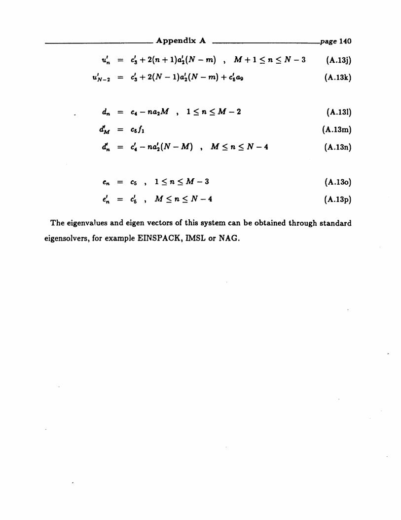
____________ Appendix A page 140
u~ - c~ + 2(n + l)a~(N - m) t M + 1 ~ n ~ N - 3 (A.13j)
U~_2 - c~ + 2(N - l)a~(N - m) + C~(Ig (A.13k)
dn - C4 - R42M 1<n<M-2 (A.131)
tiM - c6fl (A.13m)
tin - C~ - n4~(N - M) M<n<N-4 (A.13n)
e~ - C~
1<n<M-3
Af<n<N-4
(A.l30)
(A.13p)
The eigenvaJ.ues and eigen vectors of this system can be obtained through standard
eigensolvers, for example Elr~SPACK, IMSL or NAG.

Appendix B
Equations of Bending Vibrationwith Borehole Constraint
The equations of motion of bending vibration of the BHA are shown in equation
3.1 and 3.2. If the collar is forced to be in contact with the wall, then the following
relationship holds
x - A sin 'Y
y - a cos')'
(B.la)
(B.lh)
Recall that ~ is the clearance between the collar and the wall, 'Y is the angle from
the collar to its original unbent configuration. Note that 'Y is a function of the vertical
axis z, and time t. From equation B.la, the spatial derivatives with respect to vertical
axis, z, can be written as follows:
ax- -iJz
82x8z2 -asx
8zs -84zOZ4
-
(B.2a)
(B.2b)
(B.2c)
141

__________ Appendix B ___________page 142
If similar differentiation is carried out on equation B.th, then
ax8z
a2x8z2
asx
8zs84xoz·
(B.3a)
(B.3b)
(B.3c)
(B.3d)
IT the nonlinear terms involving the product of the differentials are neglected in
equation B.2d and B.3d, and substituting these expressions into the equation 3.1 and
3.2, and adding these two equations together, we find
a2~ a4~ApCM6. 8t2 (cos "y + sin "y) + El6.(cos "y + sin "y) 8z4
Q(sin "y - cos "y) ~:~ + (CE + C1) 6. (cos "y + sin "y) ~;
+ Apgh cos 4>1 (I - z)6. (cos "y + sin "y) ~:~ - 6.(cos "y + sin "y) ~:1
+ Apgh sin cP sin 1 = 0 (B.4)
IT we further assume that 'Y is small, then equation B.4 can be written as follows:
(B.5)
This equation is almost same as equation 3.3, except for the last term, which involving
the the clearance and the slant angle of the borehole. This term representing the effect
of the gravity on the constraint dynamics. It is sD:nilar to the effect of a spring, and
is proportional to the angle 'Y.

Appendix C
Green Function of a RotatingBealD with Linearly VaryingTension
The equation of motion of bending vibration with respect to a rota.ting reference
frame, with rotational speed n, is equation 3.8, as repeated here with variable sectional
properties
8 2 8 2r'A(z)P(~)CM(z)r' + (CE(z) + C](z) + i20A(z)p(z)CM(z))r' + 8z2 (E(z)I(z) 8z
2)
+ :z (T(z) ~~) - (02- iCE(z)O)r' = f(z, t) (C.l)
Boundary conditions for single span pinned-p!nned beam are
a2r'(O,t)r'(O, t) = 0, 8z2 = 0
82r'(L, t)r'(L, t) =0, 8z' =°
If the following notations are used:
~(z) - Jt(z)p(z) ClAf(z)
d(z) - CB(Z) + 01(%) + i20A(z)p(Z)CM(Z)
(C.2a)
(C.2b)
(0.3a)
(C.3b)
and the equation C.I is normalized with iCSpect to following va..riables: wg = ::~,
z r' .to = L' T = wot, and r = L' where subscript "0" denotes the values at a reference
143
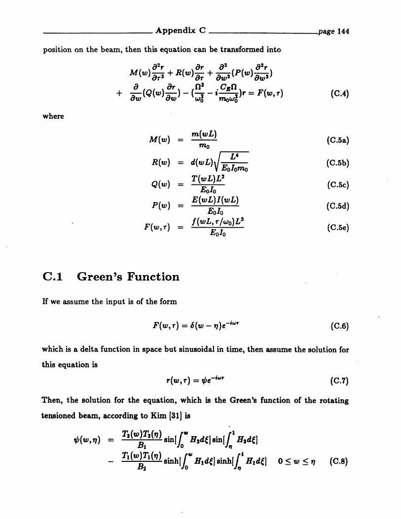
__________ Appendix C ------ page 144
position on the beam, then this equation can be transformed into
{J2r 8r 8 2 8 2rM(w)OT2 +R(W)OT + ow2 (P(W)Ow 2 )
a 8r n2 .CBO(0.4)+ -(Q(w)-) - (- -I-)r = F(W,T)
8w 8w w~ mow~
where
M(w)m(wL)
(O.Sa)-mo
R(w) ~ (C.Sb)- d(wL) E lo orno
Q(w)T(wL)L2
(C.Sc)-Eo10
P(w) E(wL)l(wL)(C.5d)-
Eo10
F(W,T)f(wL, ,,/wo)LS
(C.Se)-Eo10
C.I Green's Function
If we assume the input is of the form
F(w,,,) = 6(w - fJ)e-iwf" (C.6)
which is a delta function in space but sinusoidal in time, then assume the solution for
this equation is
(C.7)
Then, the solution for the equation, which is the Green's function of the rotating
tensioned beam, according to Kim [31] is
,pew, '1) - T2(Wff,'2('1) Sinll- H2de] Sinl£1 H 2de]
- Tl(W~~l('1) sinhllw
HIde] sinh[£1 HIde] 0 <w < '1 (C.S)

and
t1J(w, '1) - T2(W~~2('1) Sinlk" H2deJsinlLI H2del
- TI(W~~I('1) sinhlk" Hlde)8inhlLI Hide] '1 <w< 1 (C.9)
where
T1(w) 1 1 Q s (QU 1 Q 2 U t ! (C.IOa)- -[-(-) + 2 -) + -((-) + 4-) ]...;p 2 P p2 2 P P
T2(w)1 1 Q s QU 1 Q 2 U a I
(C.IOb)- -[--(-) - 2(-) + -((-) + 4-)1]i..;p 2 P p2 2 P P
H1 (w) -1 Q l yQ U
(C.IOc)-(-l+- (-)2+4-2 P 2 P P
H2 (w) -1 Q l yQ U
(C.IOd)--(-)+- (-)2+4-2 P 2 P P
B1 - sin(folH2de) (C.IOe)
B2 - sinh(fol Hide) (C.IOf)
U M( ) 2 °R() 02
° CEO (C.IOg)- w w - 1 W W - -2 +1--2Wo mowo
This Green's function is the first order approximatit>n to the exact solution obtained
using perturbation techniques.