Benchmarking Single-Image Reflection Removal Algorithms

Renjie Wan†,§,∗ Boxin Shi‡,∗ Ling-Yu Duan♦ Ah-Hwee Tan¶ Alex C. Kot§

†Interdisciplinary Graduate School, §School of Electrical and Electronic Engineering,¶School of Computer Science and Engineering, Nanyang Technological University, Singapore

‡Artificial Intelligence Research Center, National Institute of AIST, Japan♦Institute of Digital Media, Peking University, China

rjwan001@e.ntu.edu.sg, boxin.shi@aist.go.jp, lingyu@pku.edu.cn, {asahtan,eackot}@ntu.edu.sg

Abstract

Removing undesired reflections from a photo taken in

front of a glass is of great importance for enhancing the

efficiency of visual computing systems. Various approach-

es have been proposed and shown to be visually plausible

on small datasets collected by their authors. A quantitative

comparison of existing approaches using the same dataset

has never been conducted due to the lack of suitable bench-

mark data with ground truth. This paper presents the first

captured SIngle-image Reflection Removal dataset ‘SIR2’

with 40 controlled and 100 wild scenes, ground truth of

background and reflection. For each controlled scene, we

further provide ten sets of images under varying aperture

settings and glass thicknesses. We perform quantitative and

visual quality comparisons for four state-of-the-art single-

image reflection removal algorithms using four error met-

rics. Open problems for improving reflection removal algo-

rithms are discussed at the end.

1. Introduction

How to obtain a reflection-free image taken through the

glass is of great interests to computer vision researchers.

Removing the undesired reflection not only enhances the

visibility of target object, but also benefits various com-

puter vision tasks, such as image classification [29]. The

mixture image is composed of two components, the back-

ground target objects behind the glass and the reflected ob-

jects in front of the glass, in a weighted additive manner.

Reflection removal aims at separating the reflection (while

obtaining the clear background) from the mixture image us-

ing one or more shots, where the former is a highly ill-posed

problem. The reflection removal problem can be solved by

exploring gradient distribution using a single image [16],

∗Corresponding authors

motion cues from an image sequence [36], or physics con-

straint from polarized light [14]. Almost all existing works

evaluate the separation quality by checking subjective visu-

al quality; quantitative evaluation is performed only using

synthetic data, but seldom on real data due to the lack of ap-

propriate dataset. Benchmark datasets have been served as

stimuli to future research for various physics-based vision

problems such as intrinsic image decomposition [11] and

photometric stereo [28]. This motivates us to benchmark

reflection removal algorithms.

This paper starts from a brief survey of existing reflec-

tion removal algorithms. We categorize existing method-

s according to different number of images required as in-

put. Multiple images or special hardware makes reflec-

tion removal less ill-posed and show more promising results

than the single-image approaches. But the single-image ap-

proach still attracts great attention due to its simplicity in

setup and practicability for non-professional users. There-

fore, we propose the SIR2 benchmark dataset and evalua-

tions focusing on the single-image methods using different

priors and constraints.

Our SIR2 dataset contains a total of 1, 500 images. We

capture 40 controlled indoor scenes with complex textures,

and each scene contains a triplet of images (mixture image,

ground truth of background and reflection) under seven dif-

ferent depth of field and three controlled thickness of glass.

We also capture 100 wild scenes with different camera set-

tings, uncontrolled illuminations and thickness of glass. We

conduct quantitative evaluations for state-of-the-art single-

image reflection removal algorithms [17, 21, 29, 34] using

four different error metrics. We analyze the pros and cons

per method and per error metric and the consistencies be-

tween quantitative results and visual qualities. The major

contributions of our work are summarized as follows:

• Benchmark dataset. We construct the first dataset

for the quantitative evaluations of single-image reflec-

tion removal algorithms with ground truth for 140 d-

3922

DOF

Camera

Physical model Mathematical model

Type -レ

Type -ロ

Type -ヮ

��岫�岻 ��岫�岻�岫�岻

��岫�岻 ��岫�岻�岫�岻

��岫�岻 ��岫�岻�岫�岻

Glass

Lens

ReflectionsReflected objectBackground object

� = �

� = ℎ

� = 糠�怠 + 紅�態

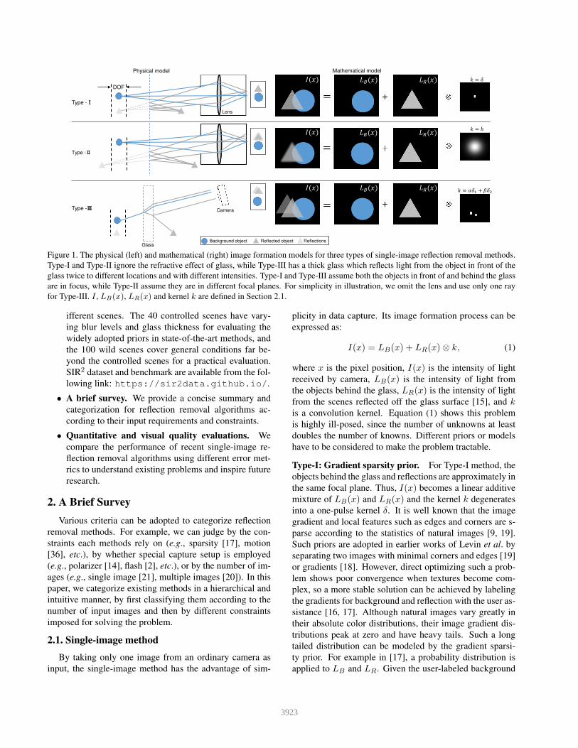
Figure 1. The physical (left) and mathematical (right) image formation models for three types of single-image reflection removal methods.

Type-I and Type-II ignore the refractive effect of glass, while Type-III has a thick glass which reflects light from the object in front of the

glass twice to different locations and with different intensities. Type-I and Type-III assume both the objects in front of and behind the glass

are in focus, while Type-II assume they are in different focal planes. For simplicity in illustration, we omit the lens and use only one ray

for Type-III. I , LB(x), LR(x) and kernel k are defined in Section 2.1.

ifferent scenes. The 40 controlled scenes have vary-

ing blur levels and glass thickness for evaluating the

widely adopted priors in state-of-the-art methods, and

the 100 wild scenes cover general conditions far be-

yond the controlled scenes for a practical evaluation.

SIR2 dataset and benchmark are available from the fol-

lowing link: https://sir2data.github.io/.

• A brief survey. We provide a concise summary and

categorization for reflection removal algorithms ac-

cording to their input requirements and constraints.

• Quantitative and visual quality evaluations. We

compare the performance of recent single-image re-

flection removal algorithms using different error met-

rics to understand existing problems and inspire future

research.

2. A Brief Survey

Various criteria can be adopted to categorize reflection

removal methods. For example, we can judge by the con-

straints each methods rely on (e.g., sparsity [17], motion

[36], etc.), by whether special capture setup is employed

(e.g., polarizer [14], flash [2], etc.), or by the number of im-

ages (e.g., single image [21], multiple images [20]). In this

paper, we categorize existing methods in a hierarchical and

intuitive manner, by first classifying them according to the

number of input images and then by different constraints

imposed for solving the problem.

2.1. Single­image method

By taking only one image from an ordinary camera as

input, the single-image method has the advantage of sim-

plicity in data capture. Its image formation process can be

expressed as:

I(x) = LB(x) + LR(x)⊗ k, (1)

where x is the pixel position, I(x) is the intensity of light

received by camera, LB(x) is the intensity of light from

the objects behind the glass, LR(x) is the intensity of light

from the scenes reflected off the glass surface [15], and k

is a convolution kernel. Equation (1) shows this problem

is highly ill-posed, since the number of unknowns at least

doubles the number of knowns. Different priors or models

have to be considered to make the problem tractable.

Type-I: Gradient sparsity prior. For Type-I method, the

objects behind the glass and reflections are approximately in

the same focal plane. Thus, I(x) becomes a linear additive

mixture of LB(x) and LR(x) and the kernel k degenerates

into a one-pulse kernel δ. It is well known that the image

gradient and local features such as edges and corners are s-

parse according to the statistics of natural images [9, 19].

Such priors are adopted in earlier works of Levin et al. by

separating two images with minimal corners and edges [19]

or gradients [18]. However, direct optimizing such a prob-

lem shows poor convergence when textures become com-

plex, so a more stable solution can be achieved by labeling

the gradients for background and reflection with the user as-

sistance [16, 17]. Although natural images vary greatly in

their absolute color distributions, their image gradient dis-

tributions peak at zero and have heavy tails. Such a long

tailed distribution can be modeled by the gradient sparsi-

ty prior. For example in [17], a probability distribution is

applied to LB and LR. Given the user-labeled background

3923

edges EB and reflection edges ER, LB and LR can be esti-

mated by maximizing:

P (LB , LR) = P1(LB) · P2(LR), (2)

where P is the joint probability distribution and P1 and P2

are the distributions imposed on LB and LR. When Equa-

tion (2) is expanded, EB and ER are imposed on two penal-

ty terms. In [17], P1 and P2 are two same narrow Gaussian

distributions.

Type-II: Layer smoothness analysis. It is more reason-

able to assume that the reflections and objects behind the

glass have different distances from the camera, and taking

the objects behind the glass in focus is a common behavior.

In such a case, the observed image I is an additive mixture

of the background and the blurred reflections. The kernel k

depends on the point spread function of the camera which

is parameterized by a 2D Gaussian function denoted as h.

The differences in smoothness of the background and

reflection provide useful cues to perform the automatic

labelling and replace the labor-intensive operation in the

Type-I method, i.e., sharp edges are annotated as back-

ground (EB) while blurred edges are annotated as reflec-

tion (ER). There are methods using the gradient values di-

rectly [5] and analyzing gradient profile sharpness [37], and

exploring DoF confidence map to perform the edge classifi-

cation [34].

The methods mentioned above all share the same recon-

struction step as [17], which means they impose the same

distributions (P1 = P2) on the gradients of LB and L̂R

(a blurred version of LR). This is not true for real scenar-

ios, because for two components with different blur levels

the sharp component LB usually has more abrupt changes

in gradient than the blurred component L̂R. Li et al. [21]

introduced a more general statistical model by assuming

P1 6= P2. P1 is designed for the large gradient values, so it

drops faster than P2 which is for the small gradient values.

Type-III: Ghosting effect. Both types above assume the

refractive effect of glass is negligible, while a more real-

istic physics model should also take the thickness of glass

into consideration. As illustrated in Figure 1 Type-III, light

rays from the objects in front of the glass are partially re-

flected on the outside facet of the glass, and the remaining

rays penetrate the glass and reflected again from the insid-

e facet of the glass. Such ghosting effects caused by the

thick glass make the observed image I a mixture of LB

and the convolution of LR with a two-pulse ghosting ker-

nel k = αδ1 + βδ2, where α and β are the combination

coefficients and δ2 is a spatial shift of δ1. Shih et al. [29]

adopted such an image formation model, and they used a

GMM model to capture the structure of the reflection.

2.2. Multiple­image method

Though much progress has been made in single-image

solutions, the limitations are also obvious due to the chal-

lenging nature of this problem: Type-I methods may not

work well if the mixture image contains many intersection-

s of edges from both layers; Type-II methods require the

smoothness and sharpness of the two layers are clearly dis-

tinguishable; Type-III methods need to estimate the ghost-

ing kernel by using the autocorrelation map which may fail

on images with strong globally repetitive textures. Multiple

images captured in various ways could significantly make

the reflection removal problem more tractable.

The first category of multiple-image methods exploit-

s the motion cues between the background and reflection

using at least three images of the same scene from differ-

ent viewpoints. Assuming the glass is closer to the cam-

era, the projected motion of the background and reflection

is different due to the visual parallax. The motion of each

layer can be represented using parametric models, such as

the translative motion [4], the affine transformation [10]

and the homography [12]. In contrast to the fixed para-

metric motion, dense motion fields provide a more general

modeling of layer motions represented by per-pixel motion

vectors. Existing reflection removal methods estimate the

dense motion fields for each layer using optical flow [33],

SIFT flow [20, 31, 30], and the pixel-wise flow field [36].

The second category of multiple-image methods can

be represented as a linear combination of the background

and reflection: The i-th image is represented as Ii(x) =αiLB(x) + βiLR(x), where combination coefficients αi

and βi can be estimated by taking a sequence of images

using special devices or in different environments, e.g., by

rotating the polarizer [8, 26, 6, 14, 23], repetitive dynamic

behaviors [24], and different illuminations [7].

The third category of multiple-image methods takes a

set of images under special conditions and camera settings,

such as using flash and non-flash image pair [2, 1], different

focuses [25], light field camera [35], and two images taken

by the front and back camera of a mobile phone [13].

Due to the additional information from multiple images,

the problem becomes less ill-posed or even well-posed.

However, special data capture requirements such as observ-

ing different layer motions or the demand for special equip-

ment such as the polarizer largely limit such methods for

practical use, especially for mobile devices or images down-

loaded from the Internet.

3. Benchmark Dataset

According to the categorization in Section 2, the

multiple-image methods usually request different setups for

input data capture (e.g., motion, polarizer, etc.); thus it

is challenging to benchmark them using the same dataset.

3924

Wild Scene Controlled Scene

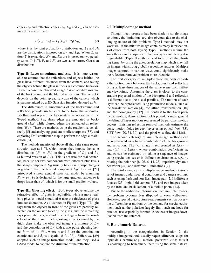
Figure 2. An overview of the SIR2 dataset: Triplet of images for 50 (selected from 100, see supplementary material for complete examples)

wild scenes (left) and 40 controlled scenes (right). Please zoom in the electronic version for better details.

� �� ��F11 / T5 F19 / T5 F32 / T5

F32 / T3 F32 / T5 F32 / T10

… …

F-v

aria

nce

T-v

aria

nce

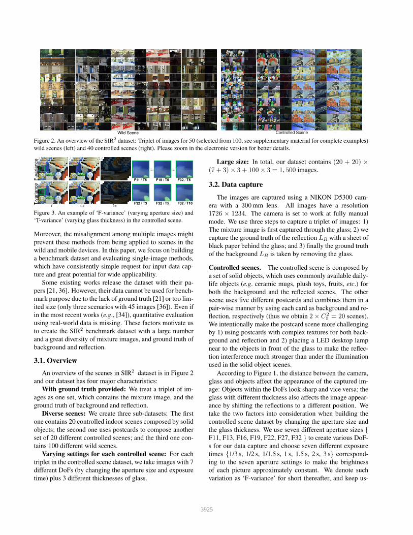
Figure 3. An example of ‘F-variance’ (varying aperture size) and

‘T-variance’ (varying glass thickness) in the controlled scene.

Moreover, the misalignment among multiple images might

prevent these methods from being applied to scenes in the

wild and mobile devices. In this paper, we focus on building

a benchmark dataset and evaluating single-image methods,

which have consistently simple request for input data cap-

ture and great potential for wide applicability.

Some existing works release the dataset with their pa-

pers [21, 36]. However, their data cannot be used for bench-

mark purpose due to the lack of ground truth [21] or too lim-

ited size (only three scenarios with 45 images [36]). Even if

in the most recent works (e.g., [34]), quantitative evaluation

using real-world data is missing. These factors motivate us

to create the SIR2 benchmark dataset with a large number

and a great diversity of mixture images, and ground truth of

background and reflection.

3.1. Overview

An overview of the scenes in SIR2 dataset is in Figure 2

and our dataset has four major characteristics:

With ground truth provided: We treat a triplet of im-

ages as one set, which contains the mixture image, and the

ground truth of background and reflection.

Diverse scenes: We create three sub-datasets: The first

one contains 20 controlled indoor scenes composed by solid

objects; the second one uses postcards to compose another

set of 20 different controlled scenes; and the third one con-

tains 100 different wild scenes.

Varying settings for each controlled scene: For each

triplet in the controlled scene dataset, we take images with 7

different DoFs (by changing the aperture size and exposure

time) plus 3 different thicknesses of glass.

Large size: In total, our dataset contains (20 + 20) ×(7 + 3)× 3 + 100× 3 = 1, 500 images.

3.2. Data capture

The images are captured using a NIKON D5300 cam-

era with a 300mm lens. All images have a resolution

1726 × 1234. The camera is set to work at fully manual

mode. We use three steps to capture a triplet of images: 1)

The mixture image is first captured through the glass; 2) we

capture the ground truth of the reflection LR with a sheet of

black paper behind the glass; and 3) finally the ground truth

of the background LB is taken by removing the glass.

Controlled scenes. The controlled scene is composed by

a set of solid objects, which uses commonly available daily-

life objects (e.g. ceramic mugs, plush toys, fruits, etc.) for

both the background and the reflected scenes. The other

scene uses five different postcards and combines them in a

pair-wise manner by using each card as background and re-

flection, respectively (thus we obtain 2× C2

5= 20 scenes).

We intentionally make the postcard scene more challenging

by 1) using postcards with complex textures for both back-

ground and reflection and 2) placing a LED desktop lamp

near to the objects in front of the glass to make the reflec-

tion interference much stronger than under the illumination

used in the solid object scenes.

According to Figure 1, the distance between the camera,

glass and objects affect the appearance of the captured im-

age: Objects within the DoFs look sharp and vice versa; the

glass with different thickness also affects the image appear-

ance by shifting the reflections to a different position. We

take the two factors into consideration when building the

controlled scene dataset by changing the aperture size and

the glass thickness. We use seven different aperture sizes {F11, F13, F16, F19, F22, F27, F32 } to create various DoF-

s for our data capture and choose seven different exposure

times {1/3 s, 1/2 s, 1/1.5 s, 1 s, 1.5 s, 2 s, 3 s} correspond-

ing to the seven aperture settings to make the brightness

of each picture approximately constant. We denote such

variation as ‘F-variance’ for short thereafter, and keep us-

3925

�� Difference map�Figure 4. Image alignment of our dataset. The first row and sec-

ond row are the images before and after registration, respectively.

Please refer to the supplementary material for more results.

ing the same glass with a thickness of 5mm when vary-

ing DoF. To explore how different thickness of glass affects

the effectives of existing methods, we place three different

glass with thickness of {3 mm, 5 mm, 10 mm} (denoted as

{T3, T5, T10} and ‘T-variance’ for short thereafter) one by

one during the data capture under a fixed aperture size F32

and exposure time 3 s. As shown in Figure 3, for the ‘F-

variance’, the reflections taken under F32 are the sharpest,

and the reflections taken under F11 have the greatest blur.

For the ‘T-variance’, the reflections taken with T10 and T3

shows largest and smallest spatial shift, respectively.

Wild scenes. The controlled scene dataset is purposely

designed to include the common priors with varying pa-

rameters for a thorough evaluation of state-of-the-art meth-

ods (e.g. [34, 29, 21, 17]). But real scenarios have much

more complicated environments: Most of the objects in our

dataset are diffuse, but objects with complex reflectance

properties are quite common; real scene contains various

depth and distance variation at multiple scales, while the

controlled scene contains only flat objects (postcard) or ob-

jects with similar scales (solid objects); natural environment

illumination also varies greatly, while the controlled scenes

are mostly captured in an indoor office environment. To ad-

dress these limitations of the controlled scene dataset, we

bring our setup out of the lab to capture a wild scene dataset

with real-world objects of complex reflectance (car, tree

leaves, glass windows, etc.), various distances and scales

(residential halls, gardens,and lecture rooms, etc.), and d-

ifferent illuminations (direct sunlight, cloudy sky light and

twilight, etc.). It is obvious that night scene (or scene with

dark background) contains much stronger reflections. So

we roughly divide the wild scene dataset into bright and

dark scenes since they bring different levels of difficulty to

the reflection removal algorithms with each set containing

50 scenes, respectively.

3.3. Image alignment

The pixel-wise alignment between the mixture image

and the ground truth is necessary to accurately perform

quantitative evaluation. During the data capture, we have

tried our best to get avoid of the object and camera motion-

s, by placing the objects on a solid platform and control-

ling the camera with a remote computer. However, due to

the refractive effect of the glass, the spatial shifts still exist

between the ground truth of background taken without the

glass and the mixture image taken with the glass, especially

when the glass is thick.

Some existing methods [6, 27] ignore such spatial shift

when they perform the quantitative evaluation. But as a

benchmark dataset, we need highly accurate alignment.

Though the refractive effect introduces complicated motion,

we find that a global projective transformation works well

for our problem. We first extract SURF feature points [3]

from two images, and then estimate the homographic trans-

formation matrix by using the RANSAC algorithm. Finally,

the mixture image is aligned to the ground truth of back-

ground with the estimated transformation. Figure 4 shows

an example of a image pair before and after alignment.

4. Evaluation

In this section, we use the SIR2 dataset to evaluate

representative single-image reflection removal algorithms,

AY07 [17], LB14 [21], SK15 [29], and WS16 [34], for both

quantitative accuracy (w.r.t. to our ground truth) and visual

quality. We choose these four methods, because they are re-

cent methods belonging to different types according to Sec-

tion 2.1 with state-of-the-art performance.

For each evaluated method, we use default parameter-

s suggested in their papers or used in their original codes.

AY07 [17] requires the user labels of background and re-

flection edges, so we follow their guidance to do the anno-

tation manually. SK15 [29] requires a pre-defined threshold

(set as 70 in their code) to choose some local maxima val-

ues. However, such a default threshold shows degenerated

results on our dataset, and we manually adjust this threshold

for different images to make sure that a similar number of

local maxima values to their original demo are generated.

To make the image size compatible to all evaluated algo-

rithms, we resize all images to 400× 540.

4.1. Quantitative evaluation

Quantitative evaluation is performed by checking the d-

ifference between the ground truth of background LB and

the estimated background L∗

Bfrom each method.

Error metrics. The most straightforward way to compare

two images is to calculate their pixel-wise difference using

PSNR or MSE (e.g., in [29]). However, absolute differ-

ence such as MSE and PSNR is too strict since a single

incorrectly classified edge can often dominant the error val-

ue. Therefore, we adopt the local MSE (LMSE) [11] as

our first metric: It evaluates the local structure similarity by

calculating the similarity of each local patch. To make the

3926

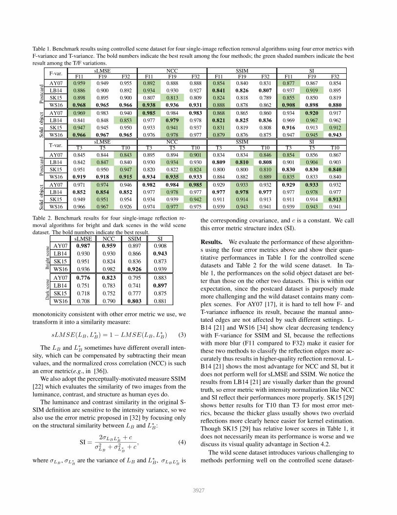
Table 1. Benchmark results using controlled scene dataset for four single-image reflection removal algorithms using four error metrics with

F-variance and T-variance. The bold numbers indicate the best result among the four methods; the green shaded numbers indicate the best

result among the T/F variations.

sLMSE NCC SSIM SIF11 F19 F32 F11 F19 F32 F11 F19 F32 F11 F19 F32

AY07 0.959 0.949 0.955 0.892 0.888 0.888 0.854 0.840 0.831 0.877 0.867 0.854

LB14 0.886 0.900 0.892 0.934 0.930 0.927 0.841 0.826 0.807 0.937 0.919 0.895

SK15 0.898 0.895 0.900 0.807 0.813 0.809 0.824 0.818 0.789 0.855 0.850 0.819

WS16 0.968 0.965 0.966 0.938 0.936 0.931 0.888 0.878 0.862 0.908 0.898 0.880

AY07 0.969 0.983 0.940 0.985 0.984 0.983 0.868 0.865 0.860 0.934 0.920 0.917

LB14 0.841 0.848 0.853 0.977 0.979 0.978 0.821 0.825 0.836 0.969 0.967 0.962

SK15 0.947 0.945 0.950 0.933 0.941 0.937 0.831 0.819 0.808 0.916 0.913 0.912

WS16 0.966 0.967 0.965 0.976 0.978 0.977 0.879 0.876 0.875 0.947 0.945 0.943

sLMSE NCC SSIM SIT3 T5 T10 T3 T5 T10 T3 T5 T10 T3 T5 T10

AY07 0.845 0.844 0.843 0.895 0.894 0.901 0.834 0.834 0.846 0.854 0.856 0.867

LB14 0.842 0.847 0.840 0.930 0.934 0.930 0.809 0.810 0.808 0.901 0.904 0.903

SK15 0.951 0.950 0.947 0.820 0.822 0.824 0.800 0.800 0.810 0.830 0.830 0.840

WS16 0.919 0.918 0.915 0.934 0.935 0.933 0.884 0.882 0.889 0.835 0.833 0.840

AY07 0.971 0.974 0.946 0.982 0.984 0.985 0.929 0.933 0.932 0.929 0.933 0.932

LB14 0.852 0.854 0.852 0.977 0.978 0.977 0.977 0.978 0.977 0.977 0.978 0.977

SK15 0.949 0.951 0.954 0.934 0.939 0.942 0.911 0.914 0.913 0.911 0.914 0.913

WS16 0.966 0.967 0.926 0.974 0.977 0.975 0.939 0.943 0.941 0.939 0.943 0.941

F-var.

T-var.

Post

card

Solid

obje

ct

Post

card

Solid

obje

ct

Table 2. Benchmark results for four single-image reflection re-

moval algorithms for bright and dark scenes in the wild scene

dataset. The bold numbers indicate the best result.

Bri

gh

t sc

ene

Dar

k s

cen

e

sLMSE NCC SSIM SI

AY07 0.987 0.959 0.897 0.908

LB14 0.930 0.930 0.866 0.943

SK15 0.951 0.824 0.836 0.873

WS16 0.936 0.982 0.926 0.939

AY07 0.776 0.823 0.795 0.883

LB14 0.751 0.783 0.741 0.897

SK15 0.718 0.752 0.777 0.875

WS16 0.708 0.790 0.803 0.881

monotonicity consistent with other error metric we use, we

transform it into a similarity measure:

sLMSE(LB , L∗

B) = 1− LMSE(LB , L

∗

B) (3)

The LB and L∗

Bsometimes have different overall inten-

sity, which can be compensated by subtracting their mean

values, and the normalized cross correlation (NCC) is such

an error metric(e.g., in [36]).

We also adopt the perceptually-motivated measure SSIM

[22] which evaluates the similarity of two images from the

luminance, contrast, and structure as human eyes do.

The luminance and contrast similarity in the original S-

SIM definition are sensitive to the intensity variance, so we

also use the error metric proposed in [32] by focusing only

on the structural similarity between LB and L∗

B:

SI =2σLBL∗

B+ c

σ2

LB+ σ2

L∗

B

+ c, (4)

where σLB, σL∗

Bare the variance of LB and L∗

B, σLBL∗

Bis

the corresponding covariance, and c is a constant. We call

this error metric structure index (SI).

Results. We evaluate the performance of these algorithm-

s using the four error metrics above and show their quan-

titative performances in Table 1 for the controlled scene

datasets and Table 2 for the wild scene dataset. In Ta-

ble 1, the performances on the solid object dataset are bet-

ter than those on the other two datasets. This is within our

expectation, since the postcard dataset is purposely made

more challenging and the wild dataset contains many com-

plex scenes. For AY07 [17], it is hard to tell how F- and

T-variance influence its result, because the manual anno-

tated edges are not affected by such different settings. L-

B14 [21] and WS16 [34] show clear decreasing tendency

with F-variance for SSIM and SI, because the reflections

with more blur (F11 compared to F32) make it easier for

these two methods to classify the reflection edges more ac-

curately thus results in higher-quality reflection removal. L-

B14 [21] shows the most advantage for NCC and SI, but it

does not perform well for sLMSE and SSIM. We notice the

results from LB14 [21] are visually darker than the ground

truth, so error metric with intensity normalization like NCC

and SI reflect their performances more properly. SK15 [29]

shows better results for T10 than T3 for most error met-

rics, because the thicker glass usually shows two overlaid

reflections more clearly hence easier for kernel estimation.

Though SK15 [29] has relative lower scores in Table 1, it

does not necessarily mean its performance is worse and we

discuss its visual quality advantage in Section 4.2.

The wild scene dataset introduces various challenging to

methods performing well on the controlled scene dataset-

3927

Ground truth �� AY07

SSIM: 0.88sLMSE: 0.98

NCC: 0.98 SI: 0.94

SSIM: 0.89 sLMSE: 0.99

NCC: 0.98 SI: 0.95

F11/T

5F

32

/T5

F32

/T3

F32/T

10

SSIM: 0.89 sLMSE: 0.98

NCC: 0.98 SI: 0.94

SSIM: 0.87sLMSE: 0.98NCC: 0.98 SI: 0.94

LB14

SSIM: 0.66

NCC: 0.97 SI: 0.96

SSIM: 0.67

NCC: 0.97 SI: 0.96

SSIM: 0.67

NCC: 0.98 SI: 0.98

SSIM: 0.68

NCC: 0.97 SI: 0.96

SK15

SSIM: 0.85

NCC: 0.96 SI: 0.92

SSIM: 0.86

NCC: 0.96 SI: 0.93

SSIM: 0.83

NCC: 0.96 SI: 0.90

SSIM: 0.85

NCC: 0.95 SI: 0.93

WS16

SSIM: 0.89

NCC: 0.98 SI: 0.94

SSIM: 0.91

NCC: 0.98 SI: 0.95

SSIM: 0.92

NCC: 0.98 SI: 0.96

SSIM: 0.92

NCC: 0.98 SI: 0.95

sLMSE: 0.92

sLMSE: 0.92

sLMSE: 0.92

sLMSE: 0.90

sLMSE: 0.96

sLMSE: 0.95

sLMSE: 0.98

sLMSE: 0.99

sLMSE: 0.99

sLMSE: 0.98

sLMSE: 0.98

sLMSE: 0.98

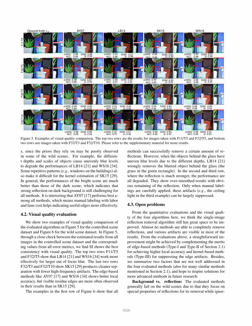
Figure 5. Examples of visual quality comparison. The top two rows are the results for images taken with F11/T5 and F32/T5, and bottom

two rows use images taken with F32/T3 and F32/T10. Please refer to the supplementary material for more results.

s, since the priors they rely on may be poorly observed

in some of the wild scenes. For example, the differen-

t depths and scales of objects cause unevenly blur levels

to degrade the performances of LB14 [21] and WS16 [34].

Some repetitive patterns (e.g., windows on the buildings) al-

so make it difficult for the kernel estimation of SK15 [29].

In general, the performances of the bright scene are much

better than those of the dark scene, which indicates that

strong reflection on dark background is still challenging for

all methods. It is interesting that AY07 [17] performs best a-

mong all methods, which means manual labeling with labor

and time cost helps indicating useful edges more effectively.

4.2. Visual quality evaluation

We show two examples of visual quality comparison of

the evaluated algorithms in Figure 5 for the controlled scene

dataset and Figure 6 for the wild scene dataset. In Figure 5,

through a close check between the estimated results from all

images in the controlled scene dataset and the correspond-

ing values from all error metrics, we find SI shows the best

consistency with visual quality. The top two rows F11/T5

and F32/T5 show that LB14 [21] and WS16 [34] work more

effectively for larger out of focus blur. The last two rows

F32/T3 and F32/T10 show SK15 [29] produces cleaner sep-

aration with fewer high-frequency artifacts. The edge-based

methods like AY07 [17] and WS16 [34] shows better local

accuracy, but visible residue edges are more often observed

in their results than in SK15 [29].

The examples in the first row of Figure 6 show that all

methods can successfully remove a certain amount of re-

flections. However, when the objects behind the glass have

uneven blur levels due to the different depths, LB14 [21]

wrongly removes the blurred object behind the glass (the

grass in the green rectangle). In the second and third row,

where the reflection is much stronger, the performance are

all degraded. They show over-smoothed results with obvi-

ous remaining of the reflection. Only when manual label-

ings are carefully applied, these artifacts (e.g., the ceiling

light in the third example) can be largely suppressed.

4.3. Open problems

From the quantitative evaluations and the visual quali-

ty of the four algorithms here, we think the single-image

reflection removal algorithm still has great space to be im-

proved. Almost no methods are able to completely remove

reflections, and various artifacts are visible in most of the

results. From the evaluations above, a straightforward im-

provement might be achieved by complementing the merits

of edge-based methods (Type-I and Type-II of Section 2.1)

for achieving higher local accuracy and kernel-based meth-

ods (Type-III) for suppressing the edge artifacts. Besides,

we summarize two factors that are not well addressed in

the four evaluated methods (also for many similar methods

mentioned in Section 2.1), and hope to inspire solutions for

more advanced methods in future research:

Background vs. reflection: The evaluated methods

generally fail on the wild scenes due to that they focus on

special properties of reflections for its removal while ignor-

3928

SSIM: 0.89 sLMSE: 0.97

NCC: 0.96 SI: 0.94

SSIM: 0.67 sLMSE: 0.78

NCC: 0.83 SI: 0.90

SSIM: 0.88

NCC: 0.97 SI: 0.92

SSIM: 0.91

NCC: 0.93 SI: 0.94

Ground truth �� AY07 LB14 SK15 WS16

SSIM: 0.85 sLMSE: 0.96

NCC: 0.72 SI: 0.87

SSIM: 0.74 sLMSE: 0.89

NCC: 0.63 SI: 0.81

SSIM: 0.81 sLMSE: 0.93

NCC: 0.53 SI: 0.84

SSIM: 0.82 sLMSE: 0.95

NCC: 0.67 SI: 0.84

sLMSE: 0.96 sLMSE: 0.98

SSIM: 0.75 sLMSE: 0.77 NCC: 0.93 SI: 0.87

SSIM: 0.91 sLMSE: 0.86NCC: 0.88 SI: 0.96

SSIM: 0.77 NCC: 0.82 SI: 0.91

SSIM: 0.78 NCC: 0.88 SI: 0.91

sLMSE: 0.60 sLMSE: 0.65

Figure 6. Examples of visual quality comparison using the wild scene dataset. The first row shows the results using images from bright

scenes and the last two rows are the results using images from the dark scenes. Please refer to the supplementary material for more results.

ing the properties of the background. A widely observed

prior suitable for the reflection removal may not be suitable

for the recovery of the background layer. Future methods

may avoid the strong dependence on priors for reflection,

which may overly remove information of the background.

Local vs. global: We find that in our dataset, many re-

flections only occupy a part of the whole images. However,

most existing methods (Type-II, Type-III and the multiple-

image methods) process every part of an image, which

downgrades the quality of the regions without reflection-

s. Local reflection regions can only be roughly detected

through manually labelling (AY07 [17]). Methods that au-

tomatically detect and process the reflection regions may

have potential to improve the overall quality.

5. Conclusion

We build SIR2 — the first benchmark real image dataset

for quantitatively evaluating single-image reflection re-

moval algorithms. Our dataset consists of various scenes

with different capturing settings. We evaluated state-of-

the-art single-image algorithms using different error metrics

and compared their visual quality.

In spite of the advantages discussed previously, the lim-

itations still exist in our dataset. Since we only consider

the diversity of scenarios when capturing the wild scene

dataset, we do not control the capturing settings used in the

controlled scene dataset. It would be a little difficult to trace

what factor rally affect the performance of a method in the

wild scenes.

To address these limitations, we will continue to extend

our dataset to more diverse scenarios for the controlled and

wild scene dataset. Meanwhile, we will organize our dataset

in a more efficient way not simply divide them based on

the brightness. On the other hand, we will also provide the

complete taxonomy, dataset, and evaluation for reflection

removal in the future work.

Acknowledgement

This work is partially supported by the National Research

Foundation, Prime Ministers Office, Singapore, under the NRF-

NSFC grant NRF2016NRF-NSFC001-098; a project commis-

sioned by the New Energy and Industrial Technology Develop-

ment Organization (NEDO); and grants from National Natural Sci-

ence Foundation of China (U1611461, 61661146005). This work

was done at the Rapid-Rich Object Search (ROSE) Lab, Nanyang

Technological University, Singapore.

3929

References

[1] A. Agrawal, R. Raskar, and R. Chellappa. Edge suppres-

sion by gradient field transformation using cross-projection

tensors. In Proc. CVPR, 2006.

[2] A. Agrawal, R. Raskar, S. K. Nayar, and Y. Li. Re-

moving photography artifacts using gradient projection and

flash-exposure sampling. ACM TOG (Proc. SIGGRAPH),

24(3):828–835, 2015.

[3] H. Bay, T. Tuytelaars, and L. Van Gool. Surf: Speeded up

robust features. In Proc. ECCV, 2006.

[4] E. Be’Ery and A. Yeredor. Blind separation of superim-

posed shifted images using parameterized joint diagonaliza-

tion. IEEE TIP, 17(3):340–353, 2008.

[5] Y. C. Chung, S. L. Chang, J. Wang, and S. Chen. Interference

reflection separation from a single image. In Proc. WACV,

2009.

[6] Y. Diamant and Y. Y. Schechner. Overcoming visual rever-

berations. In Proc. CVPR, 2008.

[7] K. I. Diamantaras and T. Papadimitriou. Blind separation of

reflections using the image mixtures ratio. In Proc. ICIP,

2005.

[8] H. Farid and E. H. Adelson. Separating reflections and

lighting using independent components analysis. JOSA A,

16(9):2136–2145, 1998.

[9] R. Fergus, B. Singh, A. Hertzmann, T. Roweis, and W. Free-

man. Removing camera shake from a single photograph.

ACM TOG (Proc. SIGGRAPH), 25(3):787–794, 2006.

[10] K. Gai, Z. Shi, and C. Zhang. Blind separation of superim-

posed moving images using image statistics. IEEE TPAMI,

34(1):19–32, 2012.

[11] R. Grosse, M. K. Johnson, E. H. Adelson, and W. T. Free-

man. Ground truth dataset and baseline evaluations for in-

trinsic image algorithms. In Proc. ICCV, 2009.

[12] X. Guo, X. Cao, and Y. Ma. Robust separation of reflection

from multiple images. In Proc. CVPR, 2014.

[13] P. Kalwad, D. Prakash, V. Peddigari, and P. Srinivasa. Re-

flection removal in smart devices using a prior assisted inde-

pendent components analysis. In Electronic Imaging, pages

940405–940405. SPIE, 2015.

[14] N. Kong, Y. W. Tai, and J. S. Shin. A physically-based

approach to reflection separation: from physical modeling

to constrained optimization. IEEE TPAMI, 36(2):209–221,

2014.

[15] N. Kong, Y. W. Tai, and S. Y. Shin. A physically-based ap-

proach to reflection separation. In Proc. CVPR, 2012.

[16] A. Levin and Y. Weiss. User assisted separation of reflections

from a single image using a sparsity prior. In Proc. ECCV,

2004.

[17] A. Levin and Y. Weiss. User assisted separation of reflections

from a single image using a sparsity prior. IEEE TPAMI,

29(9):1647, 2007.

[18] A. Levin, A. Zomet, and Y. Weiss. Learning to perceive

transparency from the statistics of natural scenes. In Proc.

NIPS, 2002.

[19] A. Levin, A. Zomet, and Y. Weiss. Separating reflections

from a single image using local features. In Proc. CVPR,

2004.

[20] Y. Li and M. S. Brown. Exploiting reflection change for au-

tomatic reflection removal. In Proc. ICCV, 2013.

[21] Y. Li and M. S. Brown. Single image layer separation using

relative smoothness. In Proc. CVPR, 2014.

[22] A. Ninassi, O. Le Meur, P. Le Callet, and D. Barba. On the

performance of human visual system based image quality as-

sessment metric using wavelet domain. In SPIE Conference

Human Vision and Electronic Imaging XIII, 2008.

[23] B. Sarel and M. Irani. Separating transparent layers through

layer information exchange. In Proc. ECCV, 2004.

[24] B. Sarel and M. Irani. Separating transparent layers of repet-

itive dynamic behaviors. In Proc. ICCV, 2005.

[25] Y. Y. Schechner, N. Kiryati, and R. Basri. Separation of

transparent layers using focus. IJCV, 39(1):25–39, 2000.

[26] Y. Y. Schechner, J. Shamir, and N. Kiryati. Polarization-

based decorrelation of transparent layers: The inclination an-

gle of an invisible surface. In Proc. ICCV, 1999.

[27] Y. Y. Schechner, J. Shamir, and N. Kiryati. Polarization

and statistical analysis of scenes containing a semireflector.

JOSA A, 17(2):276–284, 2000.

[28] B. Shi, Z. Wu, Z. Mo, D. Duan, S.-K. Yeung, and P. Tan.

A benchmark dataset and evaluation for non-lambertian and

uncalibrated photometric stereo. In Proc. CVPR, 2016.

[29] Y. C. Shih, D. Krishnan, F. Durand, and W. T. Freeman. Re-

flection removal using ghosting cues. In Proc. CVPR, 2015.

[30] T. Sirinukulwattana, G. Choe, and I. S. Kweon. Reflection

removal using disparity and gradient-sparsity via smoothing

algorithm. In Proc. ICIP, 2015.

[31] C. Sun, S. Liu, T. Yang, B. Zeng, Z. Wang, and G. Liu. Auto-

matic reflection removal using gradient intensity and motion

cues. In ACM Multimedia, 2016.

[32] S. Sun, S. Fan, and Y. F. Wang. Exploiting image structural

similarity for single image rain removal. In Proc. ICIP, 2014.

[33] R. Szeliski, S. Avidan, and P. Anandan. Layer extraction

from multiple images containing reflections and transparen-

cy. In Proc. CVPR, 2000.

[34] R. Wan, B. Shi, A. H. Tan, and A. C. Kot. Depth of field

guided reflection removal. In Proc. ICIP, 2016.

[35] Q. Wang, H. Lin, Y. Ma, S. B. Kang, and J. Yu. Automat-

ic layer separation using light field imaging. arXiv preprint

arXiv:1506.04721, 2015.

[36] T. Xue, M. Rubinstein, C. Liu, and W. T. Freeman. A com-

putational approach for obstruction-free photography. ACM

TOG (Proc. SIGGRAPH), 34(4):1–11, 2015.

[37] Q. Yan, Y. Xu, X. Yang, and T. Nguyen. Separation of weak

reflection from a single superimposed image. IEEE SPL,

21(21):1173–1176, 2014.

3930