Belief Propagation for Structured Decision Making

Qiang LiuDepartment of Computer Science

University of California, IrvineIrvine, CA, 92697qliu1@ics.uci.edu

Alexander IhlerDepartment of Computer Science

University of California, IrvineIrvine, CA, 92697ihler@ics.uci.edu

Abstract

Variational inference algorithms such as be-lief propagation have had tremendous im-pact on our ability to learn and use graph-ical models, and give many insights for de-veloping or understanding exact and approx-imate inference. However, variational ap-proaches have not been widely adoped fordecision making in graphical models, oftenformulated through influence diagrams andincluding both centralized and decentralized(or multi-agent) decisions. In this work,we present a general variational frameworkfor solving structured cooperative decision-making problems, use it to propose severalbelief propagation-like algorithms, and ana-lyze them both theoretically and empirically.

1 Introduction

Graphical modeling approaches, including Bayesiannetworks and Markov random fields, have been widelyadopted for problems with complicated dependencystructures and uncertainties. The problems of learn-ing, i.e., estimating a model from data, and inference,e.g., calculating marginal probabilities or maximum aposteriori (MAP) estimates, have attracted wide at-tention and are well explored. Variational inferenceapproaches have been widely adopted as a principledway to develop and understand many exact and ap-proximate algorithms. On the other hand, the prob-lem of decision making in graphical models, sometimesformulated via influence diagrams or decision networksand including both sequential centralized decisions anddecentralized or multi-agent decisions, is surprisinglyless explored in the approximate inference community.

Influence diagrams (ID), or decision networks,[Howard and Matheson, 1985, 2005] are a graphicalmodel representation of structured decision problems

under uncertainty; they can be treated as an extensionof Bayesian networks, augmented with decision nodesand utility functions. Traditionally, IDs are used tomodel centralized, sequential decision processes under“perfect recall”, which assumes that the decision stepsare ordered in time and that all information is remem-bered across time; limited memory influence diagrams(LIMIDs) [Zhang et al., 1994, Lauritzen and Nilsson,2001] relax the perfect recall assumption, creating anatural framework for representing decentralized andinformation-limited decision problems, such as teamdecision making and multi-agent systems. Despite theclose connection and similarity to Bayes nets, IDs haveless visibility in the graphical model and automated re-seasoning community, both in terms of modeling andalgorithm development; see Pearl [2005] for an inter-esting historical perspective.

Solving an ID refers to finding decision rules that max-imize the expected utility function (MEU); this taskis significantly more difficult than standard inferenceon a Bayes net. For IDs with perfect recall, MEUcan be restated as a dynamic program, and solvedwith cost exponential in a constrained tree-width ofthe graph that is subject to the temporal ordering ofthe decision nodes. The constrained tree-width can bemuch higher than the tree-width associated with typ-ical inference, making MEU significantly more com-plex. For LIMIDs, non-convexity issues also arise,since the limited shared information and simultane-ous decisions may create locally optimal policies. Themost popular algorithm for LIMIDs is based on policy-by-policy improvement [Lauritzen and Nilsson, 2001],and provides only a “person-by-person” notion of opti-mality. Surprisingly, the variational ideas that revolu-tionized inference in Bayes nets have not been adoptedfor influence diagrams. Although there exists work ontransforming MEU problems into sequences of stan-dard marginalization problems [e.g., Zhang, 1998], onwhich variational methods apply, these methods donot yield general frameworks, and usually only workfor IDs with perfect recall. A full variational frame-

work would provide general procedures for developingefficient approximations such as loopy belief propaga-tion (BP), that are crucial for large scale problems, orproviding new theoretical analysis.

In this work, we propose a general variational frame-work for solving influence diagrams, both with andwithout perfect recall. Our results on centralized deci-sion making include traditional inference in graphicalmodels as special cases. We propose a spectrum ofexact and approximate algorithms for MEU problemsbased on the variational framework. We give severaloptimality guarantees, showing that under certain con-ditions, our BP algorithm can find the globally optimalsolution for ID with perfect recall and solve LIMIDs ina stronger locally optimal sense than coordinate-wiseoptimality. We show that a temperature parametercan also be introduced to smooth between MEU tasksand standard (easier) marginalization problems, andcan provide good solutions by annealing the tempera-ture or using iterative proximal updates.

This paper is organized as follows. Section 2 sets upbackground on graphical models, variational methodsand influence diagrams. We present our variationalframework of MEU in Section 3, and use it to developseveral BP algorithms in Section 4. We present nu-merical experiments in Section 5. Finally, we discussadditional related work in Section 6 and concluding re-marks in Section 7. Proofs and additional informationcan be found in the appendix.

2 Background

2.1 Graphical Models

Let x = {x1, x2, · · · , xn} be a random vector in X =X1× · · · ×Xn. Consider a factorized probability on x,

p(x) =1

Z

∏α∈I

ψα(xα) =1

Zexp

[∑α∈I

θα(xα)],

where I is a set of variable subsets, and ψα : Xα → R+

are positive factors; the θα(xα) = logψα(xα) are thenatural parameters of the exponential family repre-sentation; and Z =

∑x

∏α∈I ψα is the normaliza-

tion constant or partition function with Φ(θ) = logZthe log-partition function. Let θ = {θα|α ∈ I} andθ(x) =

∑α θα(xα). There are several ways to repre-

sent a factorized distribution using graphs (i.e., graphi-cal models), including Markov random fields, Bayesiannetworks, factors graphs and others.

Given a graphical model, inference refers to the pro-cedure of answering probabilistic queries. Importantinference tasks include marginalization, maximum aposteriori (MAP, sometimes called maximum proba-bility of evidence or MPE), and marginal MAP (some-

times simply MAP). All these are NP-hard in general.Marginalization calculates the marginal probabilitiesof one or a few variables, or equivalently the normal-ization constant Z, while MAP/MPE finds the modeof the distribution. More generally, marginal MAPseeks the mode of a marginal probability,

Marginal MAP: x∗ = arg maxxA

∑xB

∏α

ψα(xα),

where A,B are disjoint sets with A∪B = V ; it reducesto marginalization if A = ∅ and to MAP if B = ∅.

Marginal Polytope. A marginal polytope M is aset of local marginals τ = {τα(xα) : α ∈ I} that areextensible to a global distribution over x, that is, M ={τ | ∃ a distribution p(x), s.t.

∑xV \α

p(x) = τα(xα) }.Call P[τ ] the set of global distributions consistentwith τ ∈M; there exists a unique distribution in P[τ ]that has maximum entropy and follows the exponen-tial family form for some θ. We abuse notation todenote this unique global distribution τ(x).

A basic result for variational methods is that Φ(θ) isconvex and can be rewritten into a dual form,

Φ(θ) = maxτ∈M{〈θ, τ 〉+H(x; τ )}, (1)

where 〈θ, τ 〉 =∑x

∑α θα(xα)τα(xα) is the point-wise

inner product, and H(x; τ ) = −∑x τ(x) log τ(x) is

the entropy of distribution τ(x); the maximum of (1)is obtained when τ equals the marginals of the originaldistribution with parameter θ. See Wainwright andJordan [2008].

Similar dual forms hold for MAP and marginal MAP.Letting ΦA,B(θ) = log maxxA

∑xB

exp(θ(x)), we have[Liu and Ihler, 2011]

ΦA,B(θ) = maxτ∈M{〈θ, τ 〉+H(xB |xA ; τ )}, (2)

where H(xB |xA ; τ ) = −∑x τ(x) log τ(xB |xA) is the

conditional entropy; its appearance corresponds to thesum operators.

The dual forms in (1) and (2) are no easier to computethan the original inference. However, one can approxi-mate the marginal polytope M and the entropy in var-ious ways, yielding a body of approximate inferencealgorithms, such as loopy belief propagation (BP) andits generalizations [Yedidia et al., 2005, Wainwrightet al., 2005], linear programming solvers [e.g., Wain-wright et al., 2003b], and recently hybrid message pass-ing algorithms [Liu and Ihler, 2011, Jiang et al., 2011].

Junction Graph BP. Junction graphs provide aprocedural framework to approximate the dual (1). Acluster graph is a triple (G, C,S), where G = (V, E) isan undirected graph, with each node k ∈ V associated

with a subset of variables ck ∈ C (clusters), and eachedge (kl) ∈ E a subset skl ∈ S (separator) satisfyingskl ⊆ ck ∩ cl. We assume that C subsumes the indexset I, that is, for any α ∈ I, there exists a ck ∈ C,denoted c[α], such that α ⊆ ck. In this case, we canreparameterize θ = {θα|α ∈ I} into θ = {θck |k ∈ V}by taking θck =

∑α : c[α]=ck

θα, without changing thedistribution. A cluster graph is called a junction graphif it satisfies the running intersection property – foreach i ∈ V , the induced sub-graph consisting of theclusters and separators that include i is a connectedtree. A junction graph is a junction tree if G is tree.

To approximate the dual (1), we can replace M witha locally consistent polytope L: the set of localmarginals τ = {τck , τskl : k ∈ V, (kl) ∈ E} satisfying∑xck\skl

τck(xck) = τ(xskl). Clearly, M ⊆ L. We then

approximate (1) by

maxτ∈L{〈θ, τ 〉+

∑k∈V

H(xck ; τ ck)−∑

(kl)∈E

H(xskl ; τ skl)},

where the joint entropy is approximated by a linearcombination of the entropies of local marginals. Theapproximate objective can be solved using Lagrangemultipliers [Yedidia et al., 2005], leading to a sum-product message passing algorithm that iterativelysends messages between neighboring clusters via

mk→l(xcl) ∝∑

xck\skl

ψck(xck)m∼k\l(xcN(k)), (3)

where ψck = exp(θck), and m∼k\l is the product ofmessages into k from its neighbors N (k) except l. Atconvergence, the (locally) optimal marginals are

τck ∝ ψckm∼k and τskl ∝ mk→lml→k,

where m∼k is the product of messages into k. Max-product and hybrid methods can be derived analo-gously for MAP and marginal MAP problems.

2.2 Influence Diagrams

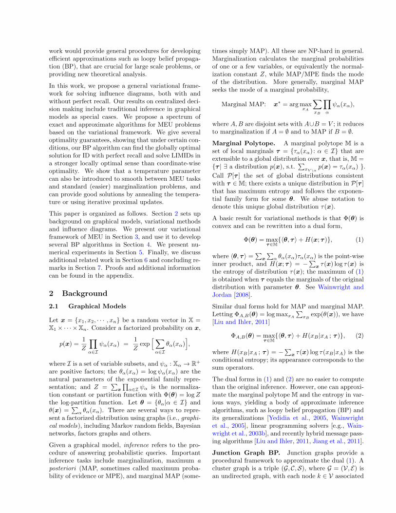
Influence diagrams (IDs) or decision networks are ex-tensions of Bayesian networks to represent structureddecision problems under uncertainty. Formally, an in-fluence diagram is defined on a directed acyclic graphG = (V,E), where the nodes V are divided into twosubsets, V = R∪D, where R and D represent respec-tively the set of chance nodes and decision nodes. Eachchance node i ∈ R represents a random variable xiwith a conditional probability table pi(xi|xpa(i)). Eachdecision node i ∈ D represents a controllable decisionvariable xi, whose value is determined by a decisionmaker via a decision rule (or policy) δi : Xpa(i) → Xi,which determines the values of xi based on the obser-vation on the values of xpa(i); we call the collection

Weather Forecast

Weather Condition

Vacation Activity Satisfaction

Chance nodes

Decision nodes

Utility nodes

Figure 1: A simple influence diagram for deciding va-cation activity [Shachter, 2007].

of policies δ = {δi|i ∈ D} a strategy. Finally, a util-ity function u : X → R+ measures the reward givenan instantiation of x = [xR, xD], which the decisionmaker wants to maximize. It is reasonable to assumesome decomposition structure on the utility u(x), ei-ther additive, u(x) =

∑j∈U uj(xβj ), or multiplicative,

u(x) =∏j∈U uj(xβj ). A decomposable utility func-

tion can be visualized by augmenting the DAG witha set of leaf nodes U , called utility nodes, each withparent set βj . See Fig. 1 for a simple example.

A decision rule δi is alternatively represented as adeterministic conditional “probability” pδi (xi|xpa(i)),

where pδi (xi|xpa(i)) = 1 for xi = δi(xpa(i)) and zerootherwise. It is helpful to allow soft decision ruleswhere pδi (xi|xpa(i)) takes fractional values; these de-fine a randomized strategy in which xi is determinedby randomly drawing from pδi (xi|xpa(i)). We denoteby ∆o the set of deterministic strategies and ∆ the setof randomized strategies. Note that ∆o is a discreteset, while ∆ is its convex hull.

Given an influence diagram, the optimal strategyshould maximize the expected utility function (MEU):

MEU = maxδ∈∆

EU(δ) = maxδ∈∆

E(u(x)|δ)

= maxδ∈∆

∑x

u(x)∏i∈C

pi(xi|xpa(i))∏i∈D

pδi (xi|xpa(i))

def= max

δ∈∆

∑x

exp(θ(x))∏i∈D

pδi (xi|xpa(i)) (4)

where θ(x) = log[u(x)∏i∈C pi(xi|xpa(i))]; we call the

distribution q(x) ∝ exp(θ(x)) the augmented distri-bution [Bielza et al., 1999]. The concept of the aug-mented distribution is critical since it completely spec-ifies a MEU problem without the semantics of the in-fluence diagram; hence one can specify q(x) arbitrarily,e.g., via an undirected MRF, extending the definitionof IDs. We can treat MEU as a special sort of “infer-ence” on the augmented distribution, which as we willshow, generalizes more common inference tasks.

In (4) we maximize the expected utility over ∆; thisis equivalent to maximizing over ∆o, since

Lemma 2.1. For any ID, maxδ∈∆EU(δ) =maxδ∈∆o EU(δ).

Perfect Recall Assumption. The MEU prob-lem can be solved in closed form if the influence di-agram satisfies a perfect recall assumption (PRA) —there exists a “temporal” ordering over all the deci-sion nodes, say {d1, d2, · · · , dm}, consistent with thepartial order defined by the DAG G, such that everydecision node observes all the earlier decision nodesand their parents, that is, {dj} ∪ pa(dj) ⊆ pa(di) forany j < i. Intuitively, PRA implies a centralized de-cision scenario, where a global decision maker sets allthe decision nodes in a predefined order, with perfectmemory of all the past observations and decisions.

With PRA, the chance nodes can be grouped by whenthey are observed. Let ri−1 (i = 1, . . . ,m) be the setof chance nodes that are parents of di but not of anydj for j < i; then both decision and chance nodes areordered by o = {r0, d1, r1, · · · , dm, rm}. The MEU andits optimal strategy for IDs with PRA can be calcu-lated by a sequential sum-max-sum rule,

MEU =∑xr0

maxxd1

∑xr1

· · ·maxxdm

∑xrm

exp(θ(x)), (5)

δ∗di(xpa(di)) = arg maxxdi

{∑xri

· · ·maxxdm

∑xrm

exp(θ(x))},

where the calculation is performed in reverse temporalordering, interleaving marginalizing chance nodes andmaximizing decision nodes. Eq. (5) generalizes theinference tasks in Section 2.1, arbitrarily interleavingthe sum and max operators. For example, marginalMAP can be treated as a blind decision problem, whereno chance nodes are observed by any decision nodes.

As in other inference tasks, the calculation of the sum-max-sum rule can be organized into local computa-tions if the augmented distribution q(x) is factorized.However, since the max and sum operators are not ex-changeable, the calculation of (5) is restricted to elimi-nation orders consistent with the “temporal ordering”.Notoriously, this “constrained” tree-width can be veryhigh even for trees. See Koller and Friedman [2009].

However, PRA is often unrealistic. First, most systemslack enough memory to express arbitrary policies overan entire history of observations. Second, many prac-tical scenarios, like team decision analysis [Detwarasitiand Shachter, 2005] and decentralized sensor networks[Kreidl and Willsky, 2006], are distributed by nature:a team of agents makes decisions independently basedon sharing limited information with their neighbors.In these cases, relaxing PRA is very important.

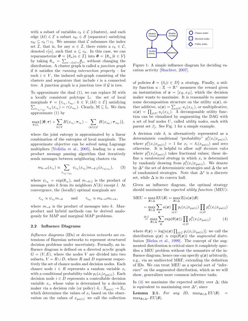
Imperfect Recall. General IDs with the perfectrecall assumption relaxed are discussed in Zhang et al.[1994], Lauritzen and Nilsson [2001], Koller and Milch[2003], and are commonly referred as limited memoryinfluence diagrams (LIMIDs). Unfortunately, the re-

d1 d2

u

d1 d2

u

d1 d2 u(d1, d2)1 1 10 1 01 0 00 0 0.5

(a) Perfect Recall (b) Imperfect Recall (c) Utility Function

Figure 2: Illustrating imperfect recall. In (a) d2 ob-serves d1; its optimal decision rule is to equal d1’s state(whatever it is); knowing d2 will follow, d1 can choosed1 = 1 to achieve the global optimum. In (b) d1 andd2 do not know the other’s states; both d1 = d2 = 1and d1 = d2 = 0 (suboptimal) become locally optimalstrategies and the problem is multi-modal.

laxation causes many difficulties. First, it is no longerpossible to eliminate the decision nodes in a sequential“sum-max-sum” fashion. Instead, the dependencies ofthe decision nodes have cycles, formally discussed inKoller and Milch [2003] by defining a relevance graphover the decision nodes; the relevance graph is a treewith PRA, but is usually loopy with imperfect recall.Thus iterative algorithms are usually required for LIM-IDs. Second and more importantly, the incomplete in-formation may cause the agents to behave myopically,selfishly choosing locally optimal strategies due to ig-norance of the global statistics. This breaks the strat-egy space into many local modes, making the MEUproblem non-convex; see Fig. 2 for an illustration.

The most popular algorithms for LIMIDs are based onpolicy-by-policy improvement, e.g., the single policyupdate (SPU) algorithm [Lauritzen and Nilsson, 2001]sequentially optimizes δi with δ¬i = {δj : j 6= i} fixed:

δi(xpa(i))← arg maxxi

E(u(x)|xfam(i) ; δ¬i), (6)

E(u(x)|xfam(i); δ¬i) =∑

x¬fam(i)

exp(θ(x))∏

j∈D\{i}

pδj(xj |xpa(j)),

where fam(i) = {i}∪pa(i). The update circles throughall i ∈ D in some order, and ties are broken arbitrar-ily in case of multiple maxima. The expected util-ity in SPU is non-decreasing at each iteration, and itgives a locally optimal strategy at convergence in thesense that the expected utility can not be improvedby changing any single node’s policy. Unfortunately,SPU’s solution is heavily influenced by initializationand can be very suboptimal.

This issue is helped by generalizing SPU to thestrategy improvement (SI) algorithm [Detwarasiti andShachter, 2005], which simultaneously updates sub-groups of decisions nodes. However, the time andspace complexity of SI grows exponentially with thesizes of subgroups. In the sequel, we present a novelvariational framework for MEU, and propose BP-likealgorithms that go beyond the naıve greedy paradigm.

3 Duality Form of MEU

In this section, we derive a duality form for MEU, gen-eralizing the duality results of the standard inferencein Section 2.1. Our main result is summarized in thefollowing theorem.

Theorem 3.1. (a). For an influence diagram withaugmented distribution q(x) ∝ exp(θ(x)), its log max-imum expected utility log MEU(θ) equals

maxτ∈M{〈θ, τ 〉+H(x; τ )−

∑i∈D

H(xi|xpa(i); τ )}. (7)

Suppose τ ∗ is a maximum of (7), then δ∗ ={τ ∗(xi|xpa(i))|i ∈ D} is an optimal strategy.

(b). For IDs with perfect recall, (7) reduces to

maxτ∈M{〈θ, τ 〉+

∑oi∈C

H(xoi |xo1:i−1; τ )}, (8)

where o is the temporal ordering of the perfect recall.

Proof. (a) See appendix; (b) note PRA implies pa(i) =o1:i−1 (i ∈ D), and apply the entropy chain rule.

The distinction between (8) and (7) is subtle but im-portant: although (8) (with perfect recall) is always(if not strictly) a convex optimization, (7) (withoutperfect recall) may be non-convex if the subtractedentropy terms overwhelm; this matches the intuitionthat incomplete information sharing gives rise to mul-tiple locally optimal strategies.

The MEU duality (8) for ID with PRA generalizes ear-lier duality results of inference: with no decision nodes,D = ∅ and (8) reduces to (1) for the log-partitionfunction; when C = ∅, no entropy terms appear and(8) reduces to the linear program relaxation of MAP.Also, (8) reduces to marginal MAP when no chancenodes are observed before any decision. As we showin Section 4, this unification suggests a line of unifiedalgorithms for all these different inference tasks.

Several corollaries provide additional insights.

Corollary 3.2. For an ID with parameter θ, we have

log MEU = maxτ∈I{〈θ, τ 〉+

∑oi∈C

H(xoi |xo1:i−1 ; τ )} (9)

where I = {τ ∈ M : xoi ⊥ xo1:i−1\pa(oi)|xpa(oi),∀oi ∈D}, corresponding to those distributions that respectthe imperfect recall constraints; “x ⊥ y | z” denotesconditional independence of x and y given z.

Corollary 3.2 gives another intuitive interpretation ofimperfect recall vs. perfect recall: MEU with imper-fect recall optimizes same objective function, but over

a subset of the marginal polytope that restricts theobservation domains of the decision rules; this non-convex inner subset is similar to the mean field approx-imation for partition functions. See Wolpert [2006] fora similar connection to mean field for bounded rationalgame theory. Interestingly, this shows that extendinga LIMID to have perfect recall (by extending the ob-servation domains of the decision nodes) can be con-sidered a “convex” relaxation of the LIMID.

Corollary 3.3. For any ε, if τ ∗ is global optimum of

maxτ∈M{〈θ, τ 〉+H(x)− (1− ε)

∑i∈D

H(xi|xpa(i))}. (10)

and δ∗ = {τ∗(xi|xpa(i))|i ∈ D} is a deterministic strat-egy, then it is an optimal strategy for MEU.

The parameter ε is a temperature to “anneal” theMEU problem, and trades off convexity and optimal-ity. For large ε, e.g., ε ≥ 1, the objective in (10) is astrictly convex function, while δ∗ is unlikely to be de-terministic nor optimal (if ε = 1, (10) reduces to stan-dard marginazation); as ε decreases towards zero, δ∗

becomes more deterministic, but (10) becomes morenon-convex and is harder to solve. In Section 4 wederive several possible optimization approaches.

4 Algorithms

The duality results in Section 3 offer new perspectivesfor MEU, allowing us to bring the tools of variationalinference to develop new efficient algorithms. In thissection, we present a junction graph framework for BP-like MEU algorithms, and provide theoretical analysis.In addition, we propose two double-loop algorithmsthat alleviate the issue of non-convexity in LIMIDs orprovide convergence guarantees: a deterministic an-nealing approach suggested by Corollary 3.3 and amethod based on the proximal point algorithm.

4.1 A Belief Propagation Algorithm

We start by formulating the problem (7) into thejunction graph framework. Let (G, C,S) be a junc-tion graph for the augmented distribution q(x) ∝exp(θ(x)). For each decision node i ∈ D, we as-sociate it with exactly one cluster ck ∈ C satisfying{i,pa(i)} ⊆ ck; we call such a cluster a decision clus-ter. The clusters C are thus partitioned into decisionclusters D and the other (normal) clusters R. Forsimplicity, we assume each decision cluster ck ∈ D isassociated with exactly one decision node, denoted dk.

Following the junction graph framework in Section 2.1,the MEU dual (10) (with temperature parameter ε) is

approximated by

maxτ∈L{〈θ, τ 〉+

∑k∈R

Hck +∑k∈D

Hεck−∑

(kl)∈E

Hskl}, (11)

where Hck = H(xck), Hskl = H(xskl) and Hε(xck) =H(xck)−(1−ε)H(xdk |xpa(dk)). The dependence of en-tropies on τ is suppressed for compactness. Eq. (11)is similar to the objective of regular sum-product junc-tion graph BP, except the entropy terms of the decisionclusters are replaced by Hε

ck.

Using a Lagrange multiplier method similar to Yedidiaet al. [2005], a hybrid message passing algorithm canbe derived for solving (11):

Sum messages:

(normal clusters)mk→l ∝

∑xck\skl

ψckm∼k\l, (12)

MEU messages:

(decision clusters)mk→l ∝

∑xck\skl

σk[ψckm∼k; ε]

ml→k, (13)

where σk[·] is an operator that solves an annealed localMEU problem associated with b(xck) ∝ ψckm∼k:

σk[b(xck); ε]def= b(xck)bε(xdk |xpa(dk))

1−ε

where bε(xdk |xpa(dk)) is the “annealed” optimal policy

bε(xdk |xpa(dk)) =b(xdk , xpa(dk))

1/ε∑xdk

b(xdk , xpa(dk))1/ε,

b(xdk , xpa(dk)) =∑xzk

b(xck), zk = ck \ {dk,pa(dk)}.

As ε→ 0+, one can show that bε(xdk |xpa(dk)) is exactlyan optimal strategy of the local MEU problem withaugmented distribution b(xck).

At convergence, the stationary point of (11) is:

τck ∝ ψckm∼k for normal clusters (14)

τck ∝ σk[ψckm∼k; ε] for decision clusters (15)

τskl ∝ mk→lml→k for separators (16)

This message passing algorithm reduces to sum-product BP when there are no decision clusters. Theoutgoing messages from decision clusters are the cru-cial ingredient, and correspond to solving local (an-nealed) MEU problems.

Taking ε→ 0+ in the MEU message update (13) givesa fixed point algorithm for solving the original objec-tive directly. Alternatively, one can adopt a deter-ministic annealing approach [Rose, 1998] by graduallydecreasing ε, e.g., taking εt = 1/t at iteration t.

Reparameterization Properties. BP algorithms,including sum-product, max-product, and hybrid mes-sage passing, can often be interpreted as reparame-terization operators, with fixed points satisfying some

sum (resp. max or hybrid) consistency property yetleaving the joint distribution unchanged [e.g., Wain-wright et al., 2003a, Weiss et al., 2007, Liu and Ih-ler, 2011]. We define a set of “MEU-beliefs” b ={b(xck), b(xskl)} by b(xck) ∝ ψckmk for all ck ∈ C, andb(xskl) ∝ mk→lml→k; note that the “beliefs” b are dis-tinguished from the “marginals” τ . We can show thatat each iteration of MEU-BP in (12)-(13), the b satisfy

Reparameterization: q(x) ∝∏k∈V b(xck)∏

(kl)∈E b(xskl), (17)

and further, at a fixed point of MEU-BP we have

Sum-consistency:

(normal clusters)

∑ck\sij

b(xck) = b(xskl), (18)

MEU-consistency:

(decision clusters)

∑ck\sij

σk[b(xck); ε] = b(xskl). (19)

Optimality Guarantees. Optimality guarantees ofMEU-BP (with ε → 0+) can be derived via reparam-eterization. Our result is analogous to those of Weissand Freeman [2001] for max-product BP and Liu andIhler [2011] for marginal-MAP.

For a junction tree, a tree-order is a partial ordering onthe nodes with k � l iff the unique path from a specialcluster (called root) to l passes through k; the parentπ(k) is the unique neighbor of k on the path to theroot. Given a subset of decision nodes D′, a junctiontree is said to be consistent for D′ if there exists atree-order with sk,π(k) ⊆ pa(dk) for any dk ∈ D′.Theorem 4.1. Let (G, C,S) be a consistent junctiontree for a subset of decision nodes D′, and b be a setof MEU-beliefs satisfying the reparameterization andconsistency conditions (17)-(19) with ε → 0+. Letδ∗ = {bck(xdk |xpa(dk)) : dk ∈ D}; then δ∗ is a locallyoptimal strategy in the sense that EU({δ∗D′ , δD\D′}) ≤EU(δ∗) for any δD\D′ .

A junction tree is said to be globally consistent if itis consistent for all the decision nodes, which as im-plied by Theorem 4.1, ensures a globally optimal strat-egy; this notation of global consistency is similar tothe strong junction trees in Jensen et al. [1994]. ForIDs with perfect recall, a globally consistent junctiontree can be constructed by a standard procedure whichtriangulates the DAG of the ID along reverse tempo-ral order. For IDs without perfect recall, it is usuallynot possible to construct a globally consistent junctiontree; this is the case for the toy example in Fig. 2b.However, coordinate-wise optimality follows as a con-sequence of Theorem 4.1 for general IDs with arbitraryjunction trees, indicating that MEU-BP is at least as“optimal” as SPU.

Theorem 4.2. Let (G, C,S) be an arbitrary junc-tion tree, and b and δ∗ defined in Theorem 4.1.Then δ∗ is a locally person-by-person optimal strategy:EU({δ∗i , δD\i}) ≤ EU(δ∗) for any i ∈ D and δD\i.

Additively Decomposable Utilities. Our al-gorithms rely on the factorization structure of theaugmented distribution q(x). For this reason, mul-tiplicative utilities fit naturally, but additive utilitiesare more difficult (as they also are in exact inference)[Koller and Friedman, 2009]. To create factorizationstructure in additive utility problems, we augment themodel with a latent “selector” variable, similar to thatin mixture models. For details, see the appendix.

4.2 Proximal Algorithms

In this section, we present a proximal point approach[e.g., Martinet, 1970, Rockafellar, 1976] for the MEUproblems. Similar methods have been applied to stan-dard inference problems, e.g., Ravikumar et al. [2010].

We start with a brief introduction to the proximalpoint algorithm. Consider an optimization problemminτ∈M f(τ ). A proximal method instead iterativelysolves a sequence of “proximal” problems

τ t+1 = arg minτ∈M

{f(τ ) + wtD(τ ||τ t)}, (20)

where τ t is the solution at iteration t and wt is a pos-itive coefficient. D(·||·) is a distance, called the prox-imal function; typical choices are Euclidean or Breg-man distances or ψ-divergences [e.g., Teboulle, 1992,Iusem and Teboulle, 1993]. Convergence of proxi-mal algorithms has been well studied: the objectiveseries {f(τ t)} is guaranteed to be non-increasing ateach iteration, and {τ t} converges to an optimal so-lution (sometimes superlinearly) for convex programs,under some regularity conditions on the coefficients{wt}. See, e.g., Rockafellar [1976], Tseng and Bert-sekas [1993], Iusem and Teboulle [1993].

Here, we use an entropic proximal function that natu-rally fits the MEU problem:

D(τ ||τ ′) =∑i∈D

∑x

τ(x) log[τi(xi|xpa(i))/τ′i(xi|xpa(i))],

a sum of conditional KL-divergences. The proximalupdate for the MEU dual (7) then reduces to

τ t+1 = arg maxτ∈M

{〈θt, τ 〉+H(x)− (1− wt)H(xi|xpa(i))}

where θt(x) = θ(x) + wt∑i∈D log τ ti (xi|xpa(i)). This

has the same form as the annealed problem (10) andcan be solved by the message passing scheme (12)-(13).Unlike annealing, the proximal algorithm updates θt

each iteration and does not need wt to approach zero.

We use two choices of coefficients {wt}: (1) wt = 1(constant), and (2) wt = 1/t (harmonic). The choicewt = 1 is especially interesting because the proximalupdate reduces to a standard marginalization prob-lem, solvable by standard tools without the MEU’stemporal elimination order restrictions. Concretely,the proximal update in this case reduces to

τ t+1i (xi|xpa(i)) ∝ τ ti (xi|xpa(i))E(u(x)|xfam(i) ; δn¬i)

with E(u(x)|xfam(i) ; δn¬i) as defined in (6). This prox-imal update can be seen as a “soft” and “parallel”version of the greedy update (6), which makes a hardupdate at a single decision node, instead of a soft mod-ification simutaneously for all decision nodes. The softupdate makes it possible to correct earlier suboptimalchoices and allows decision nodes to make cooperativemovements. However, convergence with wt = 1 maybe slow; using wt = 1/t takes larger steps but is nolonger a standard marginalization.

5 Experiments

We demonstrate our algorithms on several influence di-agrams, including randomly generated IDs, large scaleIDs constructed from problems in the UAI08 infer-ence challenge, and finally practically motivated IDsfor decentralized detection in wireless sensor networks.We find that our algorithms typically find better so-lutions than SPU with comparable time complexity;for large scale problems with many decision nodes,our algorithms are more computationally efficient thanSPU because one step of SPU requires updating (6) (aglobal expectation) for all the decision nodes.

In all experiments, we test single policy updating(SPU), our MEU-BP running directly at zero temper-ature (BP-0+), annealed BP with temperature εt =1/t (Anneal-BP-1/t), and the proximal versions withwt = 1 (Prox-BP-one) and wt = 1/t (Prox-BP-1/t).For the BP-based algorithms, we use two construc-tions of junction graphs: a standard junction tree bytriangulating the DAG in backwards topological order,and a loopy junction graph following [Mateescu et al.,2010] that corresponds to Pearl’s loopy BP; for SPU,we use the same junction graphs to calculate the in-ner update (6). The junction trees ensure the innerupdates of SPU and Prox-BP-one are performed ex-actly, and has optimality guarantees in Theorem 4.1,but may be computationally more expensive than theloopy junction graphs. For the proximal versions, weset a maximum of 5 iterations in the inner loop; chang-ing this value did not seem to lead to significantly dif-ferent results. The BP-based algorithms may returnnon-deterministic strategies; we round to determinis-tic strategies by taking the largest values.

30% 50% 70%0

0.1

0.2

Percentages of Decision Nodes

Impr

ovem

ent o

f log

ME

U

SPUBP−0+

Anneal−BP−1/tProx−BP−oneProx−BP−1/t

30% 50% 70%

−0.1

0

0.1

0.2

Percentages of Decision Nodes

(a) α = 0.3; tree (b) α = 0.3; loopy

0.3 0.5 10

0.1

0.2

Dirichlet Parameter α

Impr

ovem

ent o

f log

ME

U

0.3 0.5 1

−0.1

0

0.1

0.2

Dirichlet Parameter α

(c) 70% decision nodes; tree (d) 70% decision nodes; loopy

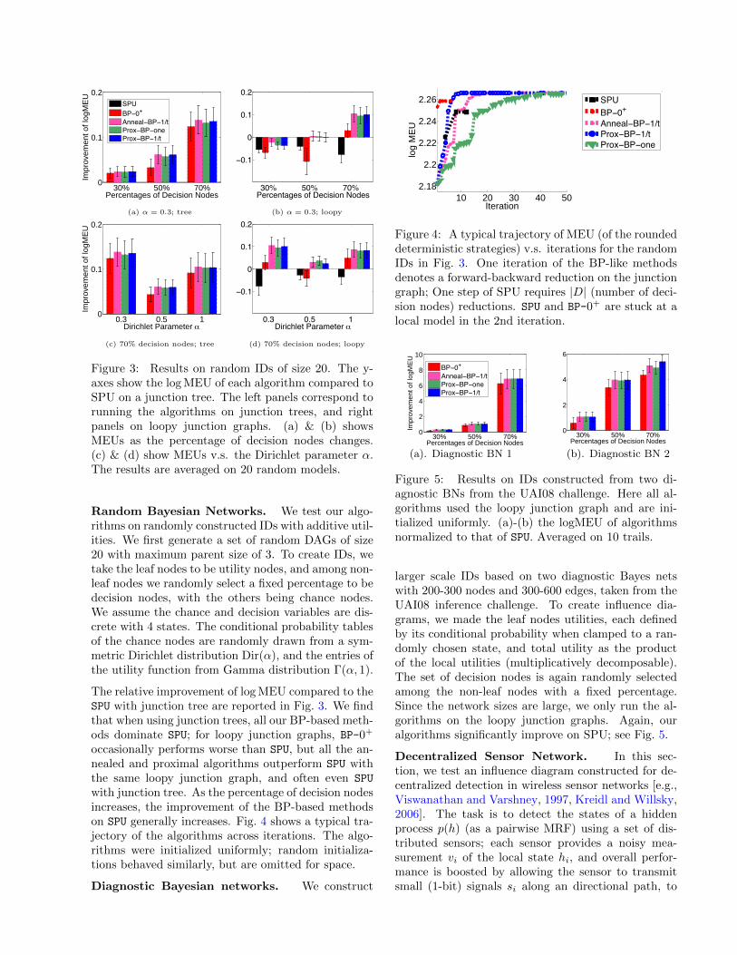
Figure 3: Results on random IDs of size 20. The y-axes show the log MEU of each algorithm compared toSPU on a junction tree. The left panels correspond torunning the algorithms on junction trees, and rightpanels on loopy junction graphs. (a) & (b) showsMEUs as the percentage of decision nodes changes.(c) & (d) show MEUs v.s. the Dirichlet parameter α.The results are averaged on 20 random models.

Random Bayesian Networks. We test our algo-rithms on randomly constructed IDs with additive util-ities. We first generate a set of random DAGs of size20 with maximum parent size of 3. To create IDs, wetake the leaf nodes to be utility nodes, and among non-leaf nodes we randomly select a fixed percentage to bedecision nodes, with the others being chance nodes.We assume the chance and decision variables are dis-crete with 4 states. The conditional probability tablesof the chance nodes are randomly drawn from a sym-metric Dirichlet distribution Dir(α), and the entries ofthe utility function from Gamma distribution Γ(α, 1).

The relative improvement of log MEU compared to theSPU with junction tree are reported in Fig. 3. We findthat when using junction trees, all our BP-based meth-ods dominate SPU; for loopy junction graphs, BP-0+

occasionally performs worse than SPU, but all the an-nealed and proximal algorithms outperform SPU withthe same loopy junction graph, and often even SPU

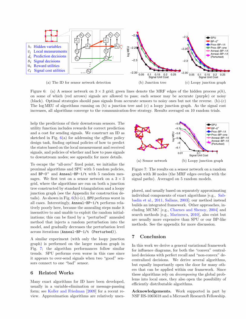
with junction tree. As the percentage of decision nodesincreases, the improvement of the BP-based methodson SPU generally increases. Fig. 4 shows a typical tra-jectory of the algorithms across iterations. The algo-rithms were initialized uniformly; random initializa-tions behaved similarly, but are omitted for space.

Diagnostic Bayesian networks. We construct

10 20 30 40 502.18

2.2

2.22

2.24

2.26

Iteration

log

ME

U

SPU

BP−0+

Anneal−BP−1/tProx−BP−1/tProx−BP−one

Figure 4: A typical trajectory of MEU (of the roundeddeterministic strategies) v.s. iterations for the randomIDs in Fig. 3. One iteration of the BP-like methodsdenotes a forward-backward reduction on the junctiongraph; One step of SPU requires |D| (number of deci-sion nodes) reductions. SPU and BP-0+ are stuck at alocal model in the 2nd iteration.

30% 50% 70%0

2

4

6

8

10

Percentages of Decision Nodes

Impr

ovem

ent o

f log

ME

U

BP−0+

Anneal−BP−1/tProx−BP−oneProx−BP−1/t

30% 50% 70%0

2

4

6

Percentages of Decision Nodes

(a). Diagnostic BN 1 (b). Diagnostic BN 2

Figure 5: Results on IDs constructed from two di-agnostic BNs from the UAI08 challenge. Here all al-gorithms used the loopy junction graph and are ini-tialized uniformly. (a)-(b) the logMEU of algorithmsnormalized to that of SPU. Averaged on 10 trails.

larger scale IDs based on two diagnostic Bayes netswith 200-300 nodes and 300-600 edges, taken from theUAI08 inference challenge. To create influence dia-grams, we made the leaf nodes utilities, each definedby its conditional probability when clamped to a ran-domly chosen state, and total utility as the productof the local utilities (multiplicatively decomposable).The set of decision nodes is again randomly selectedamong the non-leaf nodes with a fixed percentage.Since the network sizes are large, we only run the al-gorithms on the loopy junction graphs. Again, ouralgorithms significantly improve on SPU; see Fig. 5.

Decentralized Sensor Network. In this sec-tion, we test an influence diagram constructed for de-centralized detection in wireless sensor networks [e.g.,Viswanathan and Varshney, 1997, Kreidl and Willsky,2006]. The task is to detect the states of a hiddenprocess p(h) (as a pairwise MRF) using a set of dis-tributed sensors; each sensor provides a noisy mea-surement vi of the local state hi, and overall perfor-mance is boosted by allowing the sensor to transmitsmall (1-bit) signals si along an directional path, to

… si

…

vi

hi

di

ciui

…

…

dj

sj

vj

hj

uj cj

hk

vi

si

hi

di

Hidden variables Local measurements Prediction decisions Signal decisions Reward utilities Signal cost utilities ci

ui

0.05 0.1 0.15 0.2 0.25−2.35

−2.3

−2.25

−2.2

log

ME

U

Signal Unit Cost0.05 0.1 0.15 0.2 0.25

−2.35

−2.3

−2.25

−2.2

Signal Unit Cost

SPUBP−0+

Prox−BP−1/tProx−BP−oneAnneal−BP−1/tAnneal−BP−1/t(Perturbed)

(a) The ID for sensor network detection (b) Junction tree (c) Loopy junction graph

Figure 6: (a) A sensor network on 3 × 3 grid; green lines denote the MRF edges of the hidden process p(h),on some of which (red arrows) signals are allowed to pass; each sensor may be accurate (purple) or noisy(black). Optimal strategies should pass signals from accurate sensors to noisy ones but not the reverse. (b)-(c)The log MEU of algorithms running on (b) a junction tree and (c) a loopy junction graph. As the signal costincreases, all algorithms converge to the communication-free strategy. Results averaged on 10 random trials.

help the predictions of their downstream sensors. Theutility function includes rewards for correct predictionand a cost for sending signals. We construct an ID assketched in Fig. 6(a) for addressing the offline policydesign task, finding optimal policies of how to predictthe states based on the local measurement and receivedsignals, and policies of whether and how to pass signalsto downstream nodes; see appendix for more details.

To escape the “all-zero” fixed point, we initialize theproximal algorithms and SPU with 5 random policies,and BP-0+ and Anneal-BP-1/t with 5 random mes-sages. We first test on a sensor network on a 3 × 3grid, where the algorithms are run on both a junctiontree constructed by standard triangulation and a loopyjunction graph (see the Appendix for construction de-tails). As shown in Fig. 6(b)-(c), SPU performs worst inall cases. Interestingly, Anneal-BP-1/t performs rela-tively poorly here, because the annealing steps make itinsensitive to and unable to exploit the random initial-izations; this can be fixed by a “perturbed” annealedmethod that injects a random perturbation into themodel, and gradually decreases the perturbation levelacross iterations (Anneal-BP-1/t (Perturbed)).

A similar experiment (with only the loopy junctiongraph) is performed on the larger random graph inFig. 7; the algorithm performances follow similartrends. SPU performs even worse in this case sinceit appears to over-send signals when two “good” sen-sors connect to one “bad” sensor.

6 Related Works

Many exact algorithms for ID have been developed,usually in a variable-elimination or message-passingform; see Koller and Friedman [2009] for a recent re-view. Approximation algorithms are relatively unex-

0.01 0.1 1

−6.1

−6

−5.9

−5.8

−5.7

−5.6

log

ME

U

Signal Unit Cost

SPUBP−0+

Prox−BP−1/tProx−BP−oneAnneal−BP−1/tAnneal−BP−1/t(Perturbed)

(a) Sensor network (b) Loopy junction graph

Figure 7: The results on a sensor network on a randomgraph with 30 nodes (the MRF edges overlap with thesignal paths). Averaged on 5 random models.

plored, and usually based on separately approximatingindividual components of exact algorithms [e.g., Sab-badin et al., 2011, Sallans, 2003]; our method insteadbuilds an integrated framework. Other approaches, in-cluding MCMC [e.g., Charnes and Shenoy, 2004] andsearch methods [e.g., Marinescu, 2010], also exist butare usually more expensive than SPU or our BP-likemethods. See the appendix for more discussion.

7 Conclusion

In this work we derive a general variational frameworkfor influence diagrams, for both the “convex” central-ized decisions with perfect recall and “non-convex” de-centralized decisions. We derive several algorithms,but equally importantly open the door for many oth-ers that can be applied within our framework. Sincethese algorithms rely on decomposing the global prob-lems into local ones, they also open the possibility ofefficiently distributable algorithms.

Acknowledgements. Work supported in part byNSF IIS-1065618 and a Microsoft Research Fellowship.

References

C. Bielza, P. Muller, and D. R. Insua. Decision analysisby augmented probability simulation. Management Sci-ence, 45(7):995–1007, 1999.

J. Charnes and P. Shenoy. Multistage Monte Carlo methodfor solving influence diagrams using local computation.Management Science, pages 405–418, 2004.

A. Detwarasiti and R. D. Shachter. Influence diagrams forteam decision analysis. Decision Anal., 2, Dec 2005.

R. Howard and J. Matheson. Influence diagrams. In Read-ings on Principles & Appl. Decision Analysis, 1985.

R. Howard and J. Matheson. Influence diagrams. DecisionAnal., 2(3):127–143, 2005.

A. Iusem and M. Teboulle. On the convergence rate ofentropic proximal optimization methods. Computationaland Applied Mathematics, 12:153–168, 1993.

F. Jensen, F. V. Jensen, and S. L. Dittmer. From influ-ence diagrams to junction trees. In UAI, pages 367–373.Morgan Kaufmann, 1994.

J. Jiang, P. Rai, and H. Daume III. Message-passing forapproximate MAP inference with latent variables. InNIPS, 2011.

D. Koller and N. Friedman. Probabilistic graphical models:principles and techniques. MIT press, 2009.

D. Koller and B. Milch. Multi-agent influence diagrams forrepresenting and solving games. Games and EconomicBehavior, 45(1):181–221, 2003.

O. P. Kreidl and A. S. Willsky. An efficient message-passing algorithm for optimizing decentralized detectionnetworks. In IEEE Conf. Decision Control, Dec 2006.

S. Lauritzen and D. Nilsson. Representing and solving de-cision problems with limited information. ManagmentSci., pages 1235–1251, 2001.

Q. Liu and A. Ihler. Variational algorithms for marginalMAP. In UAI, Barcelona, Spain, July 2011.

R. Marinescu. A new approach to influence diagrams eval-uation. In Research and Development in Intelligent Sys-tems XXVI, pages 107–120. Springer London, 2010.

B. Martinet. Regularisation d’inequations variationnellespar approximations successives. Revue Francaise dInfor-matique et de Recherche Operationelle, 4:154–158, 1970.

R. Mateescu, K. Kask, V. Gogate, and R. Dechter. Join-graph propagation algorithms. Journal of Artificial In-telligence Research, 37:279–328, 2010.

J. Pearl. Influence diagrams - historical and personal per-spectives. Decision Anal., 2(4):232–234, dec 2005.

P. Ravikumar, A. Agarwal, and M. J. Wainwright.Message-passing for graph-structured linear programs:Proximal projections, convergence, and roundingschemes. Journal of Machine Learning Research, 11:1043–1080, Mar 2010.

R. T. Rockafellar. Monotone operators and the proximalpoint algorithm. SIAM Journal on Control and Opti-mization, 14(5):877, 1976.

K. Rose. Deterministic annealing for clustering, compres-sion, classification, regression, and related optimizationproblems. Proc. IEEE, 86(11):2210 –2239, Nov 1998.

R. Sabbadin, N. Peyrard, and N. Forsell. A framework anda mean-field algorithm for the local control of spatialprocesses. International Journal of Approximate Rea-soning, 2011.

B. Sallans. Variational action selection for influence dia-grams. Technical Report OEFAI-TR-2003-29, AustrianResearch Institute for Artificial Intelligence, 2003.

R. Shachter. Model building with belief networks and in-fluence diagrams. Advances in decision analysis: from

foundations to applications, page 177, 2007.M. Teboulle. Entropic proximal mappings with applica-

tions to nonlinear programming. Mathematics of Oper-ations Research, 17(3):pp. 670–690, 1992.

P. Tseng and D. Bertsekas. On the convergence of theexponential multiplier method for convex programming.Mathematical Programming, 60(1):1–19, 1993.

R. Viswanathan and P. Varshney. Distributed detectionwith multiple sensors: part I – fundamentals. Proc.IEEE, 85(1):54 –63, Jan 1997.

M. Wainwright and M. Jordan. Graphical models, ex-ponential families, and variational inference. Found.Trends Mach. Learn., 1(1-2):1–305, 2008.

M. Wainwright, T. Jaakkola, and A. Willsky. A new classof upper bounds on the log partition function. IEEETrans. Info. Theory, 51(7):2313–2335, July 2005.

M. J. Wainwright, T. Jaakkola, and A. S. Willsky. Tree-based reparameterization framework for analysis of sum-product and related algorithms. IEEE Trans. Info. The-ory, 45:1120–1146, 2003a.

M. J. Wainwright, T. S. Jaakkola, and A. S. Willsky. MAPestimation via agreement on (hyper) trees: Message-passing and linear programming approaches. IEEETrans. Info. Theory, 51(11):3697 – 3717, Nov 2003b.

Y. Weiss and W. Freeman. On the optimality of solutionsof the max-product belief-propagation algorithm in arbi-trary graphs. IEEE Trans. Info. Theory, 47(2):736 –744,Feb 2001.

Y. Weiss, C. Yanover, and T. Meltzer. MAP estimation,linear programming and belief propagation with convexfree energies. In UAI, 2007.

D. Wolpert. Information theory – the bridge connectingbounded rational game theory and statistical physics.Complex Engineered Systems, pages 262–290, 2006.

J. Yedidia, W. Freeman, and Y. Weiss. Constructing free-energy approximations and generalized BP algorithms.IEEE Trans. Info. Theory, 51, July 2005.

N. L. Zhang. Probabilistic inference in influence diagrams.In Computational Intelligence, pages 514–522, 1998.

N. L. Zhang, R. Qi, and D. Poole. A computational theoryof decision networks. Int. J. Approx. Reason., 11:83–158,1994.

This document contains proofs and other supplemen-tal information for the UAI 2012 submission, “BeliefPropagation for Structured Decision Making”.

A Randomized v.s. DeterministicStrategies

It is a well-known fact in decision theory that no ran-domized strategy can improve on the utility of the bestdeterministic strategy, so that:Lemma 2.1. For any ID, maxδ∈∆EU(δ) =maxδ∈∆o EU(δ).

Proof. Since ∆o ⊂ ∆, we need to show that for anyrandomized strategy δ ∈ ∆, there exists a determinis-tic strategy δ′ ∈ ∆o such that EU(δ) ≤ EU(δ′). Notethat

EU(δ) =∑x

q(x)∏i∈D

pδi (xi|xpa(i)),

Thus, EU(δ) is linear on pδi (xi|xpa(i)) for any i ∈ D(with all the other policies fixed); therefore, one canalways replace pδi (xi|xpa(i)) with some deterministic

pδ′i (xi|xpa(i)) without decreasing EU(δ). Doing so se-

quentially for all i ∈ D yields to a deterministic ruleδ′ with EU(δ) ≤ EU(δ′).

One can further show that any (globally) optimal ran-domized strategy can be represented as a convex com-bination of a set of optimal deterministic strategies.

B Duality form of MEU

Here we give a proof of our main result.Theorem 3.1. (a). For an influence diagram withaugmented distribution q(x) ∝ exp(θ(x)), its log max-imum expected utility log MEU(θ) equals

maxτ∈M{〈θ, τ 〉+H(x; τ )−

∑i∈D

H(xi|xpa(i); τ )}. (1)

Suppose τ ∗ is a maximum of (1), then δ∗ ={τ ∗(xi|xpa(i))|i ∈ D} is an optimal strategy.

(b). Under the perfect recall assumption, (1) reducesto

maxτ∈M{〈θ, τ 〉+

∑oi∈C

H(xoi |xo1:i−1; τ )} (2)

where o1:i−1 = {oj |j = 1, . . . , i− 1}.

Proof. (a). Let qδ(x) = q(x)∏i∈D p

δi (xi|xpa(i)). We

apply the standard duality result (1) of partition func-

tion on qδ(x) ∝ exp(θδ(x)),

log MEU = maxδ

log∑x

exp(θδ(x))

= maxδ

{maxτ∈M

[〈θδ, τ 〉+H(x; τ )

]}= maxτ∈M

{maxδ

[〈θδ, τ 〉

]+H(x; τ )

}, (3)

and we have

maxδ{〈θδ, τ 〉}

= maxδ{〈θ +

∑i∈D

log pδi (xi|xpa(i)), τ 〉}

= 〈θ, τ 〉+∑i∈D

maxpδi

{∑x

τ(x) log pδi (xi|xpa(i))}

∗= 〈θ, τ 〉+

∑i∈D{∑x

τ(x) log τ(xi|xpa(i))}

= 〈θ, τ 〉 −∑i∈D

H(xi|xpa(i); τ ), (4)

where the equality “∗=” holds because the solution of

maxpδi {∑x τ(x) log pδi (xi|xpa(i))} subject to the nor-

malization constraint∑xipδi (xi|xpa(i)) = 1 is pδi =

τ(xi|xpa(i)). We obtain (1) by plugging (4) into (3).

(b). By the chain rule of entropy, we have

H(x; τ ) =∑i

H(xoi |xo1:i−1; τ ). (5)

Note that we have pa(i) = o1:i−1 for i ∈ D for ID withperfect recall. The result follows by substituting (5)into (1).

The following lemma is the “dual” version ofLemma 2.1; it will be helpful for proving Corollary 3.2and Corollary 3.3.

Lemma B.1. Let Mo be the set of distributions τ(x)in which τ(xi|xpa(i)), i ∈ D are deterministic. Thenthe optimization domain M in (1) of Theorem 3.1 canbe replaced by Mo without changing the result, that is,log MEU(θ) equals

maxτ∈Mo

{〈θ, τ 〉+H(x; τ )−∑i∈D

H(xi|xpa(i); τ )}. (6)

Proof. Note that Mo is equivalent to the set of de-terministic strategies ∆o. As shown in the proof ofLemma 2.1, there always exists optimal deterministicstrategies, that is, at least one optimal solutions of (1)falls in Mo. Therefore, the result follows.

Corollary 3.2. For an ID with parameter θ, we have

log MEU = maxτ∈I{〈θ, τ 〉+

∑i∈C

H(xi|xo1:i−1 ; τ )} (7)

where I = {τ ∈ M : xoi ⊥ xo1:i−1\pa(oi)|xpa(oi)}, corre-sponding to the distributions respecting the imperfectrecall structures; “x ⊥ y | z” means that x and y areconditionally independent given z.

Proof. For any τ ∈ I, we have H(xi|xpa(i); τ ) =H(xi|xo1:i−1

; τ ), hence by the entropic chain rule, theobjective function in (7) is the same as that in (1).

Then, for any τ ∈ Mo and oi ∈ D, sinceτ(xoi |xpa(oi)) is deterministic, we have 0 ≤H(xoi |xo1:i−1

) ≤ H(xoi |xpa(oi)) = 0, which impliesI(xoi ;xo1:i\pa(oi)|xpa(oi)) = 0, and hence Mo ⊆ I ⊆M.We thus have that the LHS of (7) is no larger than(1), while no smaller than (6). The result follows since(1) and (6) equal by Lemma B.1.

Corollary 3.3. For any ε, let τ ∗ be an optimum of

maxτ∈M{〈θ, τ 〉+H(x)− (1− ε)

∑i∈D

H(xi|xpa(i))}. (8)

If δ∗ = {τ∗(xi|xpa(i))|i ∈ D} is an deterministic strat-egy, then it is an optimal strategy of the MEU.

Proof. First, we have H(xi|xpa(i); τ ) = 0 for τ ∈ Mo

and i ∈ D, since such τ(xi|xpa(i)) are determinis-tic. Therefore, the objective functions in (8) and(6) are equivalent when the maximization domainsare restricted on Mo. The result follows by applyingLemma B.1.

B.1 Derivation of Belief Propagation forMEU

Eq. (11) is similar to the objective of sum-productjunction graph BP, except the entropy terms of thedecision clusters are replaced by Hε(xck), which canbe thought of as corresponding to some local MEUproblem. In the sequel, we derive a similar belief prop-agation algorithm for (11), which requires that the de-cision clusters receive some special consideration. Todemonstrate how this can be done, we feel it is helpfulto first consider a local optimization problem associ-ated with a single decision cluster.

Lemma B.2. Consider a local optimization problemon decision cluster ck,

maxτck{〈ϑck , τck〉+Hε(xck ; τck)}.

Its solution is,

τck(xck) ∝ σk[bck(xck), ε]def= b(xck)bε(xdk |xpa(dk))

1−ε

where bck(xck) ∝ exp(ϑck(xck)) and bε(xdk |xpa(dk)) isthe “annealed” conditional probability of bck ,

bε(xdk |xpa(dk)) =b(xdk , xpa(dk))

1/ε∑xdk

b(xdk , xpa(dk))1/ε,

b(xdk , xpa(dk)) =∑xzk

b(xck), zk = ck \ {dk,pa(dk)}.

Proof. The Lagrangian function is

〈ϑck , τck〉+Hε(xck ; τck) + λ∑xck

[τck(xck)− 1].

Its stationary point satisfies

ϑck(xck)− log τck(xck)+(ε−1) log τck(xdk |xpa(dk))+λ,

or equivalently,

τck(xck)[τck(xdk |xpa(dk))]ε−1 = bck(xck). (9)

Summing over xzk on both side of (9), we have

τck(xpa(dk))[τck(xdk |xpa(dk))]ε = bck(xdk , xpa(dk)), (10)

Raising both sides of (9) to the power 1/ε and sum-ming over xdk , we have

[τck(xxpa(dk))]1/ε =

∑xdk

[bck(xdk , xpa(dk))]1/ε. (11)

Combining (11) with (10), we have

τck(xdk |xpa(dk)) = bε(xdk |xpa(dk)). (12)

Finally, combining (12) with (9) gives

τck(xck) = bck(xck)bε(xdk |xpa(dk))1−ε. (13)

The operator σk[b(xc); ε] can be treated as im-puting b(xc) with an “annealed” policy defined asbε(xdk |xpa(dk)); this can be seen more clearly in thelimit as ε→ 0+.

Lemma B.3. Consider a local MEU problem of a sin-gle decision node dk with parent nodes pa(dk) and anaugmented probability bck(xck); let

b∗(xdk |xpa(dk)) = limε→0+

bε(xdk |xpa(dk)), ∀dk ∈ D,

then δ∗ = {b∗(xdk |xpa(dk)) : dk ∈ D} is an optimalstrategy.

Proof. Let

δ∗dk(xpa(dk)) = arg maxxdk

{bε(xdk |xpa(dk))},

One can show that as ε→ 0+,

b∗(xdk |xpa(dk)) =

{1/|δ∗dk | if xdk ∈ δ∗dk0 if otherwise,

(14)

thus, b∗(xdk |xpa(dk)) acts as a “maximum operator” ofb(xdk |xpa(dk)), that is,∑xdk

b(xdk |xpa(dk))b∗(xdk |xpa(dk)) = max

xdk

b(xdk |xpa(dk)).

Therefore, for any δ ∈ ∆, we have

EU(δ) =∑xck

bck(xck)bδ(xdk |xpa(dk))

=∑

xpa(dk)

b(xpa(dk))∑xdk

b(xdk |xpa(dk))bδ(xdk |xpa(dk))

≤∑

xpa(dk)

b(xpa(dk)) maxxdk

b(xdk |xpa(dk))

=∑

xpa(dk)

b(xpa(dk))∑xdk

b(xdk |xpa(dk))b∗(xdk |xpa(dk))

= EU(δ∗).

This concludes the proof.

Therefore, at zero temperature limit, the σk[·] operatorin MEU-BP (12)-(13) can be directly calculated via(14), avoiding the necessity for power operations.

We now derive the MEU-BP in (12)-(13) for solving(11) using a Lagrange multiplier method similar toYedidia et al. [2005]. Consider the Lagrange multi-plier of (8),

〈θ, τ 〉+∑k∈R

Hck +∑k∈D

Hεck−∑

(kl)∈E

Hskl+∑(kl)∈E

∑xck\skl

λsk→l(xskl)[∑xskl

τck(xck)− τskl(xskl)],

where the nonnegative and normalization constraintsare not included and are dealt with implicitly. Tak-ing its gradient w.r.t. τck and τskl , one has

τck ∝ ψckm∼k for normal clusters, (15)

τck ∝ σk[ψckm∼k; ε] for decision clusters, (16)

τskl ∝ mk→lml→k for separators, (17)

where ψck = exp(θck), mk→l = exp(λk→l) and m∼k =∏l∈N (k)ml→k is the product of messages sending from

the set of neighboring clusters N (k) to ck. The deriva-tion of Eq. 16 used the results in Lemma B.2.

Finally, substituting the consistency constraints∑xck\skl

τck = τskl

into (15)-(17) leads the fixed point updates in (12)-(13).

B.2 Reparameterization Interpretation

We can give a reparameterization interpretation forthe MEU-BP update in (12)-(13) similar to that of thesum-, max- and hybrid- BP algorithms [e.g., Wain-wright et al., 2003a, Weiss et al., 2007, Liu and Ihler,2011]. We start by defining a set of “MEU-beliefs”b = {b(xck), b(xskl)} by b(xck) ∝ ψckmk for all ck ∈ C,and b(xskl) ∝ mk→lml→k. Note that we distinguishbetween the “beliefs” b and the “marginals” τ in (15)-(17). We have:

Lemma B.4. (a). At each iteration of MEU-BP in(12)-(13), the MEU-beliefs b satisfy

q(x) ∝∏k∈V b(xck)∏

(kl)∈E b(xskl)(18)

where q(x) is the augmented distribution of the ID.

(b). At a fixed point of MEU-BP, we have

Sum-consistency:

(normal clusters)

∑ck\sij

b(xck) = b(xskl),

MEU-consistency:

(decision clusters)

∑ck\sij

σk[b(xck); ε] = b(xskl).

Proof. (a). By simple algebraic substitution, one canshow ∏

k∈V b(xck)∏(kl)∈E b(xskl)

∝∏ck∈C

ψck(xck).

Since p(x) ∝∏ck∈C ψck(xck), the result follows.

(b). Simply substitute the definition of b into the mes-sage passing scheme (12)-(13).

B.3 Correctness Guarantees

Theorem 4.1. Let (G, C,S) be a consistent junc-tion tree for a subset of decision nodes D′, and bbe a set of MEU-beliefs satisfying the reparameteri-zation and the consistency conditions in Lemma B.4with ε → 0+. Let δ∗ = {bε(xdk |xpa(dk)) : dk ∈ D},then δ∗ is a locally optimal strategy in that sense thatEU({δ∗D′ , δD\D′}) ≤ EU(δ∗) for any δD\D′ .

Proof. On a junction tree, the reparameterization in(18) can be rewritten as

q(x) = b0∏k∈V

b(xck)

b(xsk),

where sk = sk,π(k) (sk = ∅ for the root node) and b0is the normalization constant.

For notational convenience, we only prove the casewhen D′ = D, i.e., the junction tree is globally con-sistent . More general cases follow similarly, by noting

that any decision node imputed with a fixed decisionrule can be simply treated as a chance node.

First, we can rewrite EU(δ∗) as

EU(δ∗) =∑x

q(x)∏i∈D

bε(xi|xpa(i))

= b0∑x

∏k∈V

b(xck)

b(xsk)

∏i∈D

bε(xi|xpa(i))

= b0∑x

{∏k∈C

b(xck)

b(xsk)

}·{ ∏k∈D

b(xck)bε(xdk |xpa(dk))

b(xsk)

}= b0,

where the last equality follows by the sum- and MEU-consistency condition (with ε→ 0+). To complete theproof, we just need to show that EU(δ) ≤ b0 for anyδ ∈ ∆. Again, note that EU(δ)/b0 equals

∑x

{∏k∈C

b(xck)

b(xsk)

}·{ ∏k∈D

b(xck)pδ(xdk |xpa(dk))

b(xsk)

}.

Let zk = ck \sk; since G is a junction tree, the zk forma partition of V , i.e., ∪kzk = V and zk∩zl = 1 for anyk 6= l. We have

See insert (*)

where the equality (*) holds because {zk} forms apartition of V , and equality (19) holds due to the sum-consistency condition. The last inequality follows theproof in Lemma B.3. This completes the proof.

Based to Theorem 4.1, we can easily establish person-by-person optimality of BP on an arbitrary junctiontree.

Theorem 4.2. Let (G, C,S) be an arbitrary junc-tion tree, and b and δ∗ defined in Theorem 4.1.Then δ∗ is a locally optimal strategy in Nash’s sense:EU({δ∗i , δD\i}) ≤ EU(δ∗) for any i ∈ D and δD\i.

Proof. Following Theorem 4.1, one need only showthat any junction tree is consistent for any single de-cision node i ∈ D; this is easily done by choosing atree-ordering rooted at i’s decision cluster.

C About the Proximal Algorithm

The proximal method can be equivalently interpretedas a marjorize-minimize (MM) algorithm [Hunter andLange, 2004], or a convex concave procedure [Yuille,2002]. The MM and CCCP algorithms have beenwidely applied to standard inference problems to ob-tain convergence guarantees or better solutions, seee.g., Yuille [2002], Liu and Ihler [2011].

The MM algorithm is an generalization of the EM al-gorithm, which solves minτ∈M f(τ ) by a sequence ofsurrogate optimization problems

τ t+1 = arg minτ∈M

f t(τ ),

where f t(τ ), known as a majorizing function, shouldsatisfy f t(τ ) ≥ f(τ ) for all τ ∈M and f t(τ t) = f(τ t).It is straightforward to check that the objective in theproximal update (20) is a majorizing function. There-fore, the proximal algorithm can be treated as a specialMM algorithm.

The convex concave procedure (CCCP) [Yuille andRangarajan, 2003] is a special MM algorithm whichdecomposes the objective into a difference of two con-vex functions, that is,

f(τ ) = f+(τ )− f−(τ ),

where f+(τ ) and f−(τ ) are both convex, and con-structs a majorizing function by linearizing the nega-tive part, that is,

f t(τ ) = f+(τ )−∇f−(τ t)T (τ − τ t).

One can easily show that f t(τ ) is a majorizing functionvia Jensen’s inequality. To apply CCCP on the MEUdual (1), it is natural to set

f+(τ ) = −[〈θ, τ 〉+H(x; τ )]

andf−(τ ) = −

∑i∈D

H(xi|xpa(i); τ ).

Such a CCCP algorithm is recognizable as equivalentto the proximal algorithm in Section 4.2 with wt = 1.

The convergence results for MM algorithms and CCCPare also well established; see Vaida [2005], Lange et al.[2000], Schifano et al. [2010] for the MM algorithmand Sriperumbudur and Lanckriet [2009], Yuille andRangarajan [2003] for CCCP.

D Additively Decomposable Utilities

The algorithms we describe require the augmenteddistribution q(x) to be factored, or have low (con-strained) tree-width. However, can easily not be thecase for a direct representation of additively decompos-able utilities. To explain, recall that the augmenteddistribution is q(x) ∝ q0(x)u(x), where q0(x) =∏i∈C p(xi|xpa(i)), and u(x) =

∑j∈U uj(xβj ). In this

case, the utility u(x) creates a large factor with vari-able domain ∪jβj , and can easily destroy the factoredstructure of q(x). Unfortunately, the na ive method ofcalculating the expectation node by node, or the com-monly used general variable elimination procedures

EU(δ)/b0 ≤∑x

{∏k∈C

maxxsk

b(xck)

b(xsk)

}·{ ∏k∈D

maxxsk

b(xck)pδ(xdk |xpa(dk))

b(xsk)

}(*)

=

{∏k∈C

maxxsk

∑xzk

b(xck)

b(xsk)

}·{ ∏k∈D

maxxsk

∑xzk

b(xck)pδ(xdk |xpa(dk))

b(xsk)

}(19)

=∏k∈D

maxxsk

∑xzk

b(xck)pδ(xdk |xpa(dk))

b(xsk)(20)

=∏k∈D

maxxsk

∑xdk

b(xdk , xpa(dk))pδ(xdk |xpa(dk))

b(xsk)

≤∏k∈D

maxxsk

∑xdk

b(xdk , xpa(dk))bε(xdk |xpa(dk))

b(xsk)

= 1,

[e.g., Jensen et al., 1994] do not appear suitable forour variational framework.

Instead, we introduce an artificial product structureinto the utility function by augmenting the model witha latent “selector” variable, similar to that used for the“complete likelihood” in mixture models. Let y0 be anauxiliary random variable taking values in the utilityindex set U , so that

q(x, y0) = q0(x)∏j

uj(xβj , y0),

where uj(xβj , y0) is defined by uj(xβj , j) = uj(xβj )and uj(xβj , k) = 1 for j 6= k. It is easy to verifythat the marginal distribution of q(x, y0) over y0 isq(x), that is,

∑y0q(x, y0) = q(x). The tree-width of

q(x, y0) is no larger than one plus the tree-width of thegraph (with utility nodes included) of the ID, whichis typically much smaller than that of q(x) when thecomplete utility u(x) is included directly. A deriva-tion similar to that in Theorem 3.1 shows that wecan replace θ(x) = log q(x) with θ(x) = log q(x) in(1) without changing the results. The complexity ofthis method may be further improved by exploitingthe context-specific independence of q(x, y), i.e., thatq(x|y0) has a different dependency structure for differ-ent values of y0, but we leave this for future work.

E Decentralized Sensor Network

In this section, we provide detailed information aboutthe influence diagram constructed for the decentral-ized sensor network detection problem in Section 5.Let hi, i = 1, . . . , nh, be the hidden variables we wantto detect using sensors. We assume the distribu-tion p(h) is an attractive pairwise MRF on a graph

Gh = (Vh, Eh),

p(h) =1

Zexp[

∑(ij)∈Gh

θij(hi, hj))], (21)

where hi are discrete variables with ph states (we takeph = 5); we set θij(k, k) = 0 and randomly drawθij(k, l) (k 6= l) from the negative absolute values of astandard Gaussian variable N (0, 1). Each sensor givesa noisy measurement vi of the local variable hi withprobability of error ei, that is, p(vi|hi) = 1 − ei forvi = hi and p(vi|hi) = ei/(ph − 1) (uniformly) forvi 6= hi.

Let Gs be a DAG that defines the path on which thesensors are allowed to broadcast signals (all the down-stream sensors receive the same signal); we assumethe channels are noise free. Each sensor is associatedwith two decision variables: si ∈ {0,±1} representsthe signal send from sensor i, where ±1 represents aone-bit signal with cost λ and 0 represents “off” withno cost; and di represents the prediction of hi basedon vi and the signals spas(i)

received from i’s upper-stream sensors; a correct prediction (di = hi) yieldsa reward γ (we set γ = ln 2). Hence, two types ofutility functions are involved, the signal cost utilitiesuλ, with uλ(si = ±1) = −λ and uλ(si = 0) = 0;the prediction reward utilities uγ with uγ(di, hi) = γif di = hi and uγ(di, hi) = 0 otherwise. The to-tal utility function is constructed multiplicatively viau = exp[

∑i uγ(di, hi) + uλ(si)].

We also create two qualities of sensors: “good” sen-sors for which ei are drawn from U([0, .1]) and “bad”sensors (ei ∼ U([.7, .8])), where U is the uniform dis-tribution. Generally speaking, the optimal strategiesshould pass signals from the good sensors to bad sen-sors to improve their predictive power. See Fig. 1 forthe actual influence diagram.

   

…

… i

j

k

si

…

vi

hi

di

ciui

…

…

…

dj

sj

vj

hj

uj cj

hk

vi

si

hi

di

Hidden variables Local measurements Prediction decisions Signal decisions Reward utilities Signal cost utilities ci

ui

(a) The sensor network structure (b) The influence diagram for sensor network in (a)

vihi

sivihi

vihi

s⇡(i)s⇡(i)

di

s⇡(i)

vi hi

s⇡(i)

vi hi

s⇡(i) …

vj

vk

dk

dj

sk

sj

hj

hk

s⇡(j)

s⇡(k)

h⇡0(i)

h⇡0(j) hjsj

hk

…

vj hjs⇡(j)

vj hjs⇡(j)

vjhjs⇡(j)

vjhj

s⇡(j)

vk hks⇡(k)

vk

hks⇡(k)

vk hks⇡(k)

vkhk

s⇡(k)

h⇡0(k)

sidi

dj

dk sk

sj

Decision clusters Normal clusters Separators

(c) A loopy junction graph for the ID in (b)

Figure 1: (a) A node of the sensor network structure; the green lines denote the MRF edges, on some of which (redarrows) signals are allowed to path. (b) The influence diagram constructed for the sensor network in (a). (c) A junctiongraph for the ID in (b); π(i) denotes the parent set of i in terms of the signal path Gs, and π′(i) denotes the parent setin terms of the hidden process p(h) (when p(h) is transformed into a Bayesian network by triangularizing reversely alongorder o). The decision clusters (black rectangles) are labeled with their corresponding decision variables on their top.

The definition of the ID here is not a standard one,since p(h) is not specified as a Bayesian network; butone could convert p(h) to an equivalent Bayesian net-work by the standard triangulation procedure. Thenormalization constant Z in (21) only changes the ex-pected utility function by a constant and so does notneed to be calculated for the purpose of the MEU task.

Without loss of generality, for notation we assume theorder [1, . . . , nh] is consistent with the signal path Gh.Let o = [h1, v1, d1, s1 ; . . . ; hnh , vnh , dnh , snh ]. Thejunction tree we used in the experiment is constructedby the standard triangulation procedure, backwardsalong the order o. A proper construction of a loopyjunction graph is non-trivial; we show in Fig. 1(c)the one we used in Section 5. It is constructed suchthat the decision structure inside each sensor node ispreserved to be exact, while at a higher level (amongsensors), a standard loopy junction graph (similar tothat introduced in Mateescu et al. [2010] that corre-sponds to Pearl’s loopy BP) captures the correlationbetween the sensor nodes. One can shown that such aconstructed junction graph reduces to a junction treewhen the MRF Gh is a tree and the signal path Gs isan oriented tree.

F Additional Related Work

There exists a large body of work for solving influ-ence diagrams, mostly on exact algorithms with pre-fect recall; see Koller and Friedman [2009] for a recentreview. Our work is most closely connected to theearly work of Jensen et al. [1994], who compile an IDto a junction tree structure on which a special mes-sage passing algorithm is performed; their notion ofstrong junction trees is related to our notion of globalconsistency. However, their framework requires theperfect recall assumption and it is unclear how to ex-tend it to approximate inference. A somewhat differ-ent approach transforms the decision problem into asequence of standard Bayesian network inference prob-lems [Cooper, 1988, Shachter and Peot, 1992, Zhang,1998], where each subroutine is a standard inferenceproblem, and can be solved using standard algorithms,either exactly or approximately; again, their methodonly works within the perfect recall assumption. Otherapproximation algorithms for ID are also based on ap-proximating some inner step of exact algorithms, e.g.,Sabbadin et al. [2011] and Sallans [2003] approximatethe policy update methods by mean field methods;Nath and Domingos [2010] uses adaptive belief propa-gation to approximate the inner loop of greedy searchalgorithms. [Watthayu, 2008] proposed a loopy BP al-gorithm, but without theoretical justification. To thebest of our knowledge, we know of no well-established“direct” approximation methods.

For ID without perfect recall (LIMID), backward-induction-like methods do not apply; most algorithmswork by optimizing the decision rules node-by-node orgroup-by-group; see e.g., Lauritzen and Nilsson [2001],Madsen and Nilsson [2001], Koller and Milch [2003];these methods reduce to the exact backward-reduction(hence guaranteeing global optimality) if applied onIDs with perfect recall and update backwards alongthe temporal ordering. However, they only guaranteelocal person-by-person optimality for general LIMIDs,which may be weaker than the optimality guaranteedby our BP-like methods. Other styles of approaches,such as Monte Carlo methods [e.g., Bielza et al., 1999,Cano et al., 2006, Charnes and Shenoy, 2004, Garcia-Sanchez and Druzdzel, 2004] and search-based meth-ods [e.g., Luque et al., 2008, Qi and Poole, 1995, Yuanand Wu, 2010, Marinescu, 2010] have also been pro-posed. Recently, Maua and Campos [2011] proposeda method for finding the globally optimal strategiesof LIMIDs by iteratively pruning non-maximal poli-cies. However, these methods usually appear to havemuch greater computational complexity than SPU orour BP-like methods.

Finally, some variational inference ideas have been ap-plied to the related problems of reinforcement learningor solving Markov decision processes [e,g., Sallans andHinton, 2001, Furmston and Barber, 2010, Yoshimotoand Ishii, 2004].

References

C. Bielza, P. Muller, and D. R. Insua. Decision analysisby augmented probability simulation. Management Sci-ence, 45(7):995–1007, 1999.

A. Cano, M. Gomez, and S. Moral. A forward-backwardMonte Carlo method for solving influence diagrams. Int.J. Approx. Reason., 42(1-2):119–135, 2006.

J. Charnes and P. Shenoy. Multistage Monte Carlo methodfor solving influence diagrams using local computation.Management Science, pages 405–418, 2004.

G. F. Cooper. A method for using belief networks as influ-ence diagrams. In UAI, pages 55–63, 1988.

A. Detwarasiti and R. D. Shachter. Influence diagrams forteam decision analysis. Decision Anal., 2, Dec 2005.

T. Furmston and D. Barber. Variational methods for rein-forcement learning. In AISTATS, volume 9, pages 241–248, 2010.

D. Garcia-Sanchez and M. Druzdzel. An efficient samplingalgorithm for influence diagrams. In Proceedings of theSecond European Workshop on Probabilistic GraphicalModels (PGM–04), Leiden, Netherlands, pages 97–104,2004.

R. Howard and J. Matheson. Influence diagrams. In Read-ings on Principles & Appl. Decision Analysis, 1985.

R. Howard and J. Matheson. Influence diagrams. DecisionAnal., 2(3):127–143, 2005.

D. R. Hunter and K. Lange. A tutorial on MM algorithms.The American Statistician, 1(58), February 2004.

A. Iusem and M. Teboulle. On the convergence rate ofentropic proximal optimization methods. Computational

and Applied Mathematics, 12:153–168, 1993.F. Jensen, F. V. Jensen, and S. L. Dittmer. From influ-

ence diagrams to junction trees. In UAI, pages 367–373.Morgan Kaufmann, 1994.

J. Jiang, P. Rai, and H. Daume III. Message-passing forapproximate MAP inference with latent variables. InNIPS, 2011.

D. Koller and N. Friedman. Probabilistic graphical models:principles and techniques. MIT press, 2009.

D. Koller and B. Milch. Multi-agent influence diagrams forrepresenting and solving games. Games and EconomicBehavior, 45(1):181–221, 2003.

O. P. Kreidl and A. S. Willsky. An efficient message-passing algorithm for optimizing decentralized detectionnetworks. In IEEE Conf. Decision Control, Dec 2006.

K. Lange, D. Hunter, and I. Yang. Optimization transferusing surrogate objective functions. Journal of Compu-tational and Graphical Statistics, pages 1–20, 2000.

S. Lauritzen and D. Nilsson. Representing and solving de-cision problems with limited information. ManagmentSci., pages 1235–1251, 2001.

Q. Liu and A. Ihler. Variational algorithms for marginalMAP. In UAI, Barcelona, Spain, July 2011.

M. Luque, T. Nielsen, and F. Jensen. An anytime algo-rithm for evaluating unconstrained influence diagrams.In Proc. PGM, pages 177–184, 2008.

A. Madsen and D. Nilsson. Solving influence diagramsusing HUGIN, Shafer-Shenoy and lazy propagation. InUAI, volume 17, pages 337–345, 2001.

R. Marinescu. A new approach to influence diagrams eval-uation. In Research and Development in Intelligent Sys-tems XXVI, pages 107–120. Springer London, 2010.

B. Martinet. Regularisation d’inequations variationnellespar approximations successives. Revue Francaise dInfor-matique et de Recherche Operationelle, 4:154–158, 1970.

R. Mateescu, K. Kask, V. Gogate, and R. Dechter. Join-graph propagation algorithms. Journal of Artificial In-telligence Research, 37:279–328, 2010.

D. D. Maua and C. P. Campos. solving decision problemswith limited information. In NIPS, 2011.

A. Nath and P. Domingos. Efficient belief propagation forutility maximization and repeated inference. In AAAIConference on Artificial Intelligence, 2010.

J. Pearl. Influence diagrams - historical and personal per-spectives. Decision Anal., 2(4):232–234, dec 2005.

R. Qi and D. Poole. A new method for influence diagramevaluation. Computational Intelligence, 11(3):498–528,1995.

P. Ravikumar, A. Agarwal, and M. J. Wainwright.Message-passing for graph-structured linear programs:Proximal projections, convergence, and roundingschemes. Journal of Machine Learning Research, 11:1043–1080, Mar 2010.

R. T. Rockafellar. Monotone operators and the proximalpoint algorithm. SIAM Journal on Control and Opti-mization, 14(5):877, 1976.

K. Rose. Deterministic annealing for clustering, compres-sion, classification, regression, and related optimizationproblems. Proc. IEEE, 86(11):2210 –2239, Nov 1998.

R. Sabbadin, N. Peyrard, and N. Forsell. A framework anda mean-field algorithm for the local control of spatialprocesses. International Journal of Approximate Rea-soning, 2011.

B. Sallans. Variational action selection for influence dia-grams. Technical Report OEFAI-TR-2003-29, AustrianResearch Institute for Artificial Intelligence, 2003.

B. Sallans and G. Hinton. Using free energies to representq-values in a multiagent reinforcement learning task. InNIPS, pages 1075–1081, 2001.

E. Schifano, R. Strawderman, and M. Wells. Majorization-minimization algorithms for nonsmoothly penalized ob-jective functions. Electronic Journal of Statistics, 4:1258–1299, 2010.

R. Shachter. Model building with belief networks and in-fluence diagrams. Advances in decision analysis: fromfoundations to applications, page 177, 2007.

R. Shachter and M. Peot. Decision making using proba-bilistic inference methods. In UAI, pages 276–283, 1992.

B. Sriperumbudur and G. Lanckriet. On the convergenceof the concave-convex procedure. In NIPS, pages 1759–1767, 2009.

M. Teboulle. Entropic proximal mappings with applica-tions to nonlinear programming. Mathematics of Oper-ations Research, 17(3):pp. 670–690, 1992.

P. Tseng and D. Bertsekas. On the convergence of theexponential multiplier method for convex programming.Mathematical Programming, 60(1):1–19, 1993.

F. Vaida. Parameter convergence for EM and MM algo-rithms. Statistica Sinica, 15(3):831–840, 2005.

R. Viswanathan and P. Varshney. Distributed detectionwith multiple sensors: part I – fundamentals. Proc.IEEE, 85(1):54 –63, Jan 1997.

M. Wainwright and M. Jordan. Graphical models, ex-ponential families, and variational inference. Found.Trends Mach. Learn., 1(1-2):1–305, 2008.

M. Wainwright, T. Jaakkola, and A. Willsky. A new classof upper bounds on the log partition function. IEEETrans. Info. Theory, 51(7):2313–2335, July 2005.

M. J. Wainwright, T. Jaakkola, and A. S. Willsky. Tree-based reparameterization framework for analysis of sum-product and related algorithms. IEEE Trans. Info. The-ory, 45:1120–1146, 2003a.

M. J. Wainwright, T. S. Jaakkola, and A. S. Willsky. MAPestimation via agreement on (hyper) trees: Message-passing and linear programming approaches. IEEETrans. Info. Theory, 51(11):3697 – 3717, Nov 2003b.

W. Watthayu. Representing and solving influence diagramin multi-criteria decision making: A loopy belief prop-agation method. In International Symposium on Com-puter Science and its Applications (CSA ’08), pages 118–125, Oct. 2008.

Y. Weiss and W. Freeman. On the optimality of solutionsof the max-product belief-propagation algorithm in arbi-trary graphs. IEEE Trans. Info. Theory, 47(2):736 –744,Feb 2001.

Y. Weiss, C. Yanover, and T. Meltzer. MAP estimation,linear programming and belief propagation with convexfree energies. In UAI, 2007.

D. Wolpert. Information theory – the bridge connectingbounded rational game theory and statistical physics.Complex Engineered Systems, pages 262–290, 2006.

J. Yedidia, W. Freeman, and Y. Weiss. Constructing free-energy approximations and generalized BP algorithms.IEEE Trans. Info. Theory, 51, July 2005.

J. Yoshimoto and S. Ishii. A solving method for mdpsby minimizing variational free energy. In InternationalJoint Conference on Neural Networks, volume 3, pages1817–1822. IEEE, 2004.

C. Yuan and X. Wu. Solving influence diagrams usingheuristic search. In Proc. Symp. AI& Math, 2010.

A. L. Yuille. CCCP algorithms to minimize the Bethe andKikuchi free energies: Convergent alternatives to belief

propagation. Neural Computation, 14:2002, 2002.A. L. Yuille and A. Rangarajan. The concave-convex pro-

cedure. Neural Computation, 15:915–936, April 2003.N. L. Zhang. Probabilistic inference in influence diagrams.

In Computational Intelligence, pages 514–522, 1998.N. L. Zhang, R. Qi, and D. Poole. A computational theory

of decision networks. Int. J. Approx. Reason., 11:83–158,1994.