United States Department of Agriculture

Forest Service

Pacific Northwest Research Station

Research Paper PNW-RP-373 February 1987

Behavior of M ule Deer on the Keating Winter Range W.B. Fowler and J.E. Dealy

.. ~ ' ~ ~ I T O I ~ S •

FILE COPY

• . . : . ' - : .

• o oO ,~o • • • • • o ; ~. 'o

~ ,. ° , ° .

• ~ - ° °

• - . < : • .

;, , , ' . " . . : . • . . :. . • - .o •,

: ; . . . . • • •

, . • o . , • o • • .

I ,

~!~i~ ~"

Abstract. Fowler, W.B.; Dealy, J.E. Behavior of mule deer on the Keating Winter Range. Res. Pap. PNW-RP-373 . Portland, OR: U.S. Department of Agriculture, Forest Service, Pacific Northwest Research Station; 1987.25 p.

Summary

Observations are presented from 4 years of record, 1976 to 1979, on behavior of mule deer (Odocoileus hemionus) in relation to site variables on the Keating Winter Range in northeastern Oregon. Analyses of animal use per unit area showed that the preferential selection of cells was related primarily to static site variables and secondarily to weather. The most regularly selected and strongest predictive vari- able was distance from the valley bottom, a variable generally associated with elevation. Only during the midafternoon hours of 1400 to 1600 did dynamic weather variables contribute substantially to the variance explained by the regression equa- tions. For individual cells, animal use was controlled by snow depth and temperature.

Keywords: Animal behavior, winter range, deer (mule).

Observations are presented from 4 years of record, 1976 to 1979, on behavior of mule deer (Odocoileus hemionus) in relation to site variables on the Keating Winter Range in northeastern Oregon. Analyses of animal use per unit area for 100 cells based on landform and vegetation showed that the preferential selection of cells was related primarily to static site variables and secondly to weather. The most regularly selected and strongest predictive variable was distance from the valley bottom, a variable generally associated with elevation. Only during the midafter- noon hours of 1400 to 1600 did dynamic weather variables contribute substantially to the variance explained by the regression equations. A subset of the data was available for analyzing the use of each of the cells. Snow depth was the variable controlling animal use, except for cells in the major stream channel. There, temper- ature controlled the response, and use by deer was greater during falling temper- atures. These analyses supported visual observations that animals used more of the area during warm weather and sought out areas where snow was shallower and less crusted. Improvement of winter forage and cover is most feasible near areas of high animal use. Major improvements such as cover, fencing to control snow depth, and forage enhancement would be required to alter the preferential site selection shown by the animals. Major increases in deer population or ex- cessive use by livestock could negate such improvements.

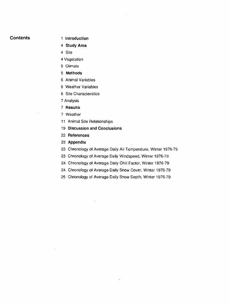
Contents 1 Introduction

4 Study Area

4 Site

4 Vegetation

5 Climate

5 Methods

6 Animal Variables

6 Weather Variables

6 Site Characteristics

7 Analysis

7 Results

7 Weather

11 Animal Site Relationships

19 Discussion and Conclusions

22 References

23 Appendix

23 Chronology of Average Daily Air Temperature, Winter 1976-79

23 Chronology of Average Daily Windspeed, Winter 1976-79

24 Chronology of Average Daily Chill Factor, Winter 1976-79

24 Chronology of Average Daily Snow Cover, Winter 1976-79

25 Chronology of Average Daily Snow Depth, Winter 1976-79

I n t r o d u c t i o n Winter is the most critical period for mule deer (Odocoileus hemionus)Non most ranges in the interior West (Connolly 1981). Deep snow restricts the available feeding area, severe weather (wind and cold) produces a yearly high in energy demands from the animals, and quality forage is at its yearly low.

As weather conditions worsen with the onset of winter in eastern Oregon, deer migrate from the forests of the Wallowa Mountains to the surrounding rangelands (fig. 1). Those moving south concentrate on the benchlands near the Powder River (fig. 2), in an area ranging from 1 to 10 miles wide by 40 miles long (1.6 to 16 km by 64 km), designated here as the Keating Winter Range.

1/Sources for scientific and common names are Garrison and others (1976) and Ingles (1965).

, Keating Winter Range

~'~ ~ ~ ~ i ~ ' , Study area _ -,. ~ . . . r~

Baker 0~~ ~

/ I

1 1 0 . 0 mi

Figure 1--Location of the Keating Winter Range in eastern Oregon.

r i ,

Figure 2--Aerial view of the study area on the Powder River. Note clearing of snow from the south-facing slopes.

The Keating Winter Range supports a population of mule deer that has ranged from 3,500 to 7,600 in recent years.~ This range generally supports deer over the winter, but with sporadic die-offs caused by severe weather and lack of adequate forage and cover. The Oregon Department of Fish and Wildlife considered the problem severe enough in the mid-1960's to develop a program of emergency feeding in winter. Although weather conditions are better in spring, the physical condition of emaciated survivors of a severe winter (fig. 3, B) will continue to dete- riorate until regrowing vegetation meets their energy needs.

During the winter of 1971-72, a combination of deeper than average snow, animals prestressed by a prolonged cold spell, and restricted forage caused high mortality, estimated at 40 percent of the local herd (see footnote 2). A number of new studies were initiated in the mid-1970's to learn how to improve the carrying capacity of this range. This paper reports on (1) our study of the relationship of wintering deer to site, weather, and forage availability; and (2) the development of a predictive model of animal occupancy to aid in selection of suitable locations for forage rehabilitation and cover plantings. Other studies have reported on selecting improved varieties for range rehabilitation (Edgerton and others 1983, Geist and Edgerton 1984), and this research continues. Hilken (1983) examined in detail the energy demands of the animal and the availability of forage on the rangelands and the historical and present relationship to domestic animals.

~W.R Humphreys, Oregon Department of Fish and Wildlife, Baker, Oregon, personal communication.

A

~, ~. ~:. ~:~.,,....'~'~: • . .~

• ~.,~._,.,~.._ ~. ~ ~ _.o, .. ,

• ~-:" " ~ ".' .-~;,-Z~,~" -. , "

Figure 3--Mortal i ty o f animals on winter ranges can run high (A), as much as 40 percent of the local herd in severe winters. A survivor (B) will not regain healthy body condit ion until adequate forage is avail- able (photos courtesy Oregon Fish and Wildlife Department).

Study Area Site

The study area (fig. 4) was located along the Powder River in Baker County in northeastern Oregon and included approximately 1,600 acres (650 ha) of benchland along the river. The study area and much of the surrounding Keating Winter Range are on lands managed by the Bureau of Land Management, U.S. Department of the Interior. The study area was representative in vegetation and topography of much of the surrounding range and supported a large population of mule deer (about 75 animals), usually visible from a high elevation observation point south of the river. Elevation ranged from 2,450 to 3,400 feet (746 to 1036 m). Slopes into the 300- to 400-foot-deep (91- to 121-m) main Powder River canyon are short and steep (commonly 60 to 80 percent), whereas the gradients of the small tributary streams that run through the gentle topography of the upland benches are more moderate as they empty into the river. Side slopes into these drainages are gentle in the northern part of the study area but steepen to 60 to 80 percent near the Powder River canyon (fig. 2).

it

bdary

$ eras

Vegetation

Figure 4 - -Map of instruments and the general study area.

Vegetation.includes big sagebrush (Artemisia tridentata Nutt.), bearded bluebunch wheatgrass (Agropyron spicatum (Pursh) Scribn. & Smith), and annual grass com- munities with very narrow stringers of streamside riparian shrubs. A large seeding of standard crested wheatgrass (Agropyron desertorum Schult.) occupied the north and upper elevation portion of the study area; approximately 20 acres (8 ha) of alfalfa (Medicago sativa L.) had been growing in the middle of the benchland below the seeding. The lower portion of the benchland was dominated by big sagebrush, with small openings of annual grass. Through disturbance, some big sagebrush areas had been converted to rabbitbrush (Chrysothamnus nauseosus (Pall.) Brit.) successional stages. At the extreme north edge of the study area, several heavily overgrazed rocky slopes supported a few small, dense stands of medusahead wildrye (Elymus caput-medusae L.).

Climate Annual precipitation averages about 16 inches (40 cm) and occurs primarily during the winter. Precipitation varies with topography; lower elevation stations to the south and west are drier than highland stations to the east and north. Snow is common, accumulating to depths up to 20 inches (50 cm), with drifts rarely ex- ceeding 40 inches (1 m).

Average daily temperatures for December through March for nearby regularly reporting stations are shown in figure 5. With the exception of Richland, mean monthly temperatures are lowest in January. Richland also is the warmest of these stations during the winter. Lengthy periods of extreme cold are infrequent, but some have lasted as long as 20 days. Minimum temperatures may drop into the -30 °F (35 °C) range locally. Minimums of -50 °F (45 °C) have been recorded at several nearby stations in eastern Oregon.

Air temperature oc OF

10- -50

Methods

S-- --4

0-

-30

a~: ; rar~oOrttatlon KBKR

o Durkee -20 • Halfway

• Richland I I I I I

DEC JAN FEB M A R

Figure 5--Average daily temperatures for nearby regularly report- ing stations; based on 10-year period, December 1966 to March 1976.

During the active period of the study, 1976 to 1979, two broad classes of dynamic or changing information were collected through ocular estimates and meteoro- logical instruments: (1) animal variables (time of day, and location and number of animals); and (2) weather variables (solar radiation, air temperature, windspeed, and wind direction). Weather data were recorded automatically at 16 locations and were complemented by general visual observation of cover and depth of snow, cloud cover, and precipitation.

Site characteristics such as aspect, slope, vegetation height, and cell coordinates were also determined.

Animal Variables

Weather Variables

Site Characteristics

Trained observers monitored animal activity 2 days per week from the observation post south of the river. By use of binoculars and spotting scopes, animals were located accurately on large-scale map.~ of the study area. Animal locations were later recorded on a 100-cell, site-specific mosaic map developed from landform and vegetation descriptions of the area. Five time-lapse movie cameras were placed in strategic locations to record deer activity at 15-minute intervals during daylight hours every day, all winter, each year of the study.

Sixteen weather statiofis were located systematically (fig. 4). These weather sta- tions were numbered and used as visual reference points for the ocular sightings of animal activity. A summary of air temperature, windspeed, and direction was printed at 20-minute intervals. Air temperature was recorded as the average temperature for the 20-minute period. Windspeed was measured for each 0.1 mile (0.16 km) of wind travel past a station, and total wind was recorded by selected windspeed class (in m/h): 0-5, 5-10, 10-15, 15-20, 20-30, and 30+. ~/

Fowler (1975, 1977) described the design and operation of the meteorological equip- ment for these weather stations in more detail. Solar radiometers were installed at 4 of the 16 weather stations. Data were coded by machine for later analysis. From the raw data on temperature and windspeed in several classes, the chill factor, average windspeed, and wind period were computed.

Snow cover was estimated in percent; snow depth was estimated and recorded in one of six classes: none, 0-15 cm, 15-30 cm, 30-45 cm, 45-60 cm, or 60+ cm; cloud cover was coded: sunny, scattered clouds, broken clouds, or overcast; and precipitation was coded: none, rain, snow, or fog.

The 100 cells for the landform and vegetation mosaic were generated from large- scale aerial photos and field sampling. Vegetation, slope, and aspect were the primary criteria. Four slope classes, four aspect classes, and 11 vegetation com- munities were recognized. Slopes were classified as 0 to 15 percent (ridgetops), 15 to 30 percent, 30 to 60 percent, and greater than 60 percent. Aspect classes were north, east, west, and south (including canyons and ridges).

3/Anemometers were calibrated in English units, and all wind in- formation is reported as m/h (miles per hour). To convert to meters per second (m/s), multiply miles per hour by 0.447.

Analysis

Results Weather

Vegetation communities were classified as:

1. Cheatgrass brome (Bromus tectorum L.). 2. Alfalfa. 3. Standard crested wheatgrass. 4. Bearded bluebunch wheatgrass/antelope bitterbrush (Purshia tridentata (Pursh)

DC.). 5. Antelope bitterbrush/bearded bluebunch wheatgrass. 6. Rabbitbrush (Chrysothamnus nauseosus (Pall.) Brit.)/bearded bluebunch

wheatgrass. 7. Big sagebrush/cheatgrass brome. 8. Antelope bitterbrush/needlegrass (Stipa sp.). 9. Big sagebrush/bearded bluebunch wheatgrass.

10. Antelope bitterbrush-rabbitbrush/bearded bluebunch wheatgrass-cheatgrass brome.

11. Rabbitbrush/bearded bluebunch wheatgrass-needlegrass.

These vegetation communities were characterized on the basis of height. Heights ranged from 0.5 foot (0.15 m) for standard crested wheatgrass to 4.25 feet (1.3 m) for the big sagebrush types.

Each cell was located by a selected central point on an X-Y grid over a map of the area. The Y direction (YDIR) represented elevation and distance from the main river valley. The X direction (XDIR) increased in value in the downstream direction of the Powder River; it had no component for elevation. Sizes of cells ranged from 0.23 acre (0.09 ha) in cell 6 to 26.66 acres (10.79 ha) in cell 85. A 180 ° "fisheye" lens was used to determine sky exposure at each instrument location.

Initial analysis of the weather data for the 1976-77 winter was made by hand calcu- lator before records were computer coded. Computer analyses were made (1) on an areawide basis (mapping of deer density in various time periods, stepwise regression of deer density as the dependent variable against site and weather variables, factor analysis on the multiyear data summaries for cells on the area); and (2) on selected individual cells (stepwise regression of animals observed vs. dynamic weather elements). Comparisons between weather elements at some sites (t-tests on means for similar time periods) and simple bivariate plots of deer density vs. other variables helped us to understand the complex interactions between site and animal use.

Solar radiation.--Daily averages for solar radiation (in Langleys) at weather sta- tion 2 during 1976-77 were: December, 177; January, 152; February, 259; and March, 320.

Temperature.--Figure 6 shows the maximum and minimum temperatures for Dec- ember 1976 and January 1977 at station 2, heavy plotted line, and a 3.6 °F (2 °C) departure from this station's temperature, light plotted lines. Locations of circles represent the temperature departure of the other weather stations from the station 2 measurement, and size of circle represents number of stations at a particular temperature. For example, all stations on December 4 had the same minimum

Temperature OF oc

50 .10

- o( ~,, Maximum

41 ' 5 o

32 p V 0

stat ions at each temperature ~ s h o w n by area of c irc les

32 0 (~ ) ' " UM

23 . -5N~ 14, .-1

oO I i ~ I 4 10 20 30 --

December 1 9 7 6 Tempera tu re

OF oC - 5 OOo,

32 ~ f {~ Max imum

23 ~ o

14

14 . . . . . . . . . . . . . . . . . . . . . 10

5 -15

-4 . -20

I I I 10 20 30

January 1 9 7 7

Figure 6--Temperature distribution for stations on the Keating Winter Range during December 1976 and January 1977. Station 2, heavy plotted line, was selected as a reference station. Light plotted lines are a 3.6 °F (2 °C) departure around station 2 value. Measurements from other stations are shown by location and size of circles.

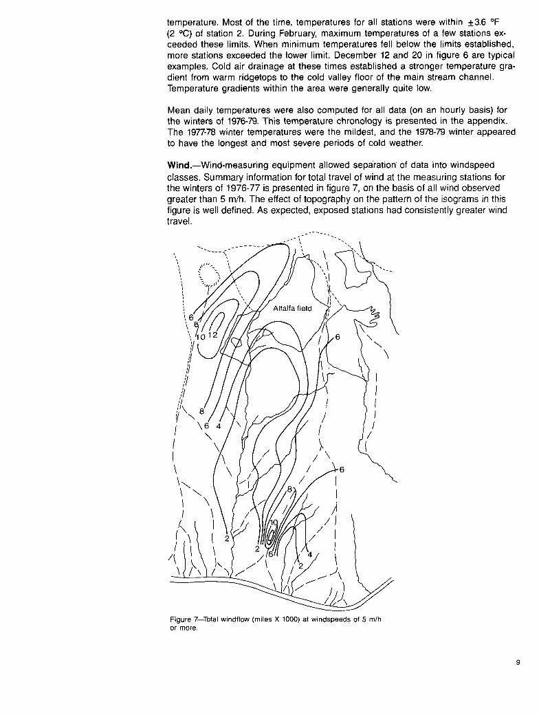
temperature. Most of the time, temperatures for all stations were within +3.6 °F (2 °C) of station 2. During February, maximum temperatures of a few stations ex- ceeded these limits. When minimum temperatures fell below the limits established, more stations exceeded the lower limit. December 12 and 20 in figure 6 are typical examples. Cold air drainage at these times established a stronger temperature gra- dient from warm ridgetops to the cold valley floor of the main stream channel. Temperature gradients within the area were generally quite low.

Mean daily temperatures were also computed for all data (on an hourly basis) for the winters of 1976-79. This temperature chronology is presented in the appendix. The 1977-78 winter temperatures were the mildest, and the 1978-79 winter appeared to have the longest and most severe periods of cold weather.

Wind.--Wind-measuring equipment allowed separation of data into windspeed classes. Summary information for total travel of wind at the measuring stations for the winters of 1976-77 is presented in figure 7, on the basis of all wind observed greater than 5 m/h. The effect of topography on the pattern of the isograms in this figure is well defined. As expected, exposed stations had consistently greater wind travel.

',\ '\ /

i J L~

? - ,

/! \

]/ I ,// I

/ I i/\\ / / /

/ / \

I

J \ i / I I} , /I I

J

Figure 7 Total windflow (miles X 1000) at windspeeds of 5 m/h or more.

The contr ibut ion of exposure to the observed run of wind at these stations was ex- amined. From both total wind and wind at speeds of 15 m/h and greater compared with percentage of sky observed at each station, the relat ionships in f igures 8 and 9 were determined. In both cases, an exponent ial curve fitted the data best, ac- count ing for 54 percent of the var iance in wind travel in f igure 8 and 62 percent in f igure 9. Attempts to improve on these relat ionships by examining exposure in various quadrants vs. windf low were not successful.

Miles x 1 0 0 0 •

12 °

x -

+

o

c

"-5 4- / -8 Y = 0-024e0136X

" " R 2 = 0.54 t- 2,- ,,,,:f:

07 I , 80 90 10O

Sky observed (percent) Figure 8--Regression of windflow (miles traveled at 5 m/h or more) on sky observed (percent) at instrument locations.

Miles x 100

28r

r-

E + LO

0

c-

0

2O

161- "

IQ 12 . .

J I.

4 / . / 010 80 90 100

Sky observed (percent) Figure 9--Regression of windflow (miles traveled at 15 m/h or more) on sky observed (percent) at instrument location.

Y = 1.346 x 109e 0"296x

R 2 = 0.62

10

Animal-Site Relationships

The constancy of wind direction during periods of light winds was normally quite poor for most areas. This relationship was therefore examined only for periods when speeds of 15 m/h or greater were recorded. The preferred direction for wind- flow during these times was generally westerly. At times, possibly associated with transition to or from cold, continental polar air from the east and more moderate maritime air masses, strong wind shifts from easterly to westerly directions or the reverse occurred. High velocity southerly or northerly winds were infrequent for the period of record in 1976-77.

Chill factor.--A critical examination of the role of wind in the determination of en- vironmental stress on animals was not possible with the data we collected. It is suf- ficient to note that the heat transfer coefficient under conditions of forced ventila- tion increases with increase of wind velocity. The ratio of this increase is on the order of the square or cube root of wind velocity (Munn 1970). High winds coupled with low air temperatures cause rapid heat loss for poorly sheltered animals. A measure of this effect is through the various chill factor expressions (Oliver 1973), which combine temperature and wind measurement.

Chill factor expressions attempt to describe numerically the discomfort accompany- ing lowering temperatures and increasing wind. Reference values and accompany- ing sensation (on humans) are shown in the following tabulation. Values are in Kcal m -2 h "1 as provided by Oliver (1973) from various sources.

Chill factor Sensation

2000 1400 1200-1400 1000-1200 800-1000 600-800

Exposed flesh freezes in 1 minute Exposed flesh freezes Bitterly cold wind chill Very cold wind chill Cold wind chill Very cool wind chill

No protracted periods of high chill factor were evident in chronologies developed for 1976-79. With the exception of several days in December 1978 when average chill factors rose to 1625 over the whole area, calculated mean values were moder- ate for the years of record, rarely above 1200.

Snow.--Daily averages of snow depth and cover based on hourly observations at all stations during the years 1976-79 are shown in the appendix. The winter of 1978-79 had the most complete and deepest snow cover, whereas the 1977-78 winter had the least cover and depth.

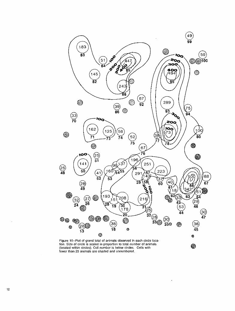
General distribution of animals.--Summary data for animal occupancy for the 1976-79 study period are shown in figures 10 and 11. Figure 10 shows the 4-year grand total of animals using designated cells. Grand total is the summation of daily means. Daily means are the total number in a cell divided by the number of obser- vations of animals in a cell. Although 100 cells were defined for the study area, only 89 were observed being used by deer. The isogram analysis indicates distribu- tion of animals was uneven over the area. Some cells along the Powder River valley bottom were not used. Because larger cells could contain more deer, animals per unit area are the basis for figure 11.

11

@

® 48

oO ,°o _@

®

@

@ 3~@ ~o

5~

@ 4 9

@

13 1 8 @

@

Figure lO--Plot of grand total of animals observed in each circle loca- tion. Size of circle is scaled in proportion to total number of animals (located within circles). Cell number is below circles. Cells with fewer than 25 animals are shaded and unnumbered.

q /

e ® 4 5

@

@

12

®

0

0

@ ®

51

/ 50 @ 52

® oo

@

76

29

@

® 95

@ 93

78

® 94

@

®

@

®®®

~ 6 / O

o ®

@

Figure 11--Plot of animals per unit area for cells.

O

The pattern of the isograms is again evident in figure 11, with a concentration of animals on the benchlands near the valley bottoms. Animals avoided the exposed ridgetops and congregated in the main stream channel central to the study area (cells 19, 28, 30), and in a shallow headwater basin (cells 61-67). Using a per-area basis puts the large and small areas in proper perspective. Distribution of animals per unit area for each year of record was also mapped, and a similar pattern was found for each year.

13

O

88

o,/ \ ®\®

O

® / ~ ® o o ) e ®

O @ @ O i

Figure 12--Plot of animals per unit area for the period 0800-1000.

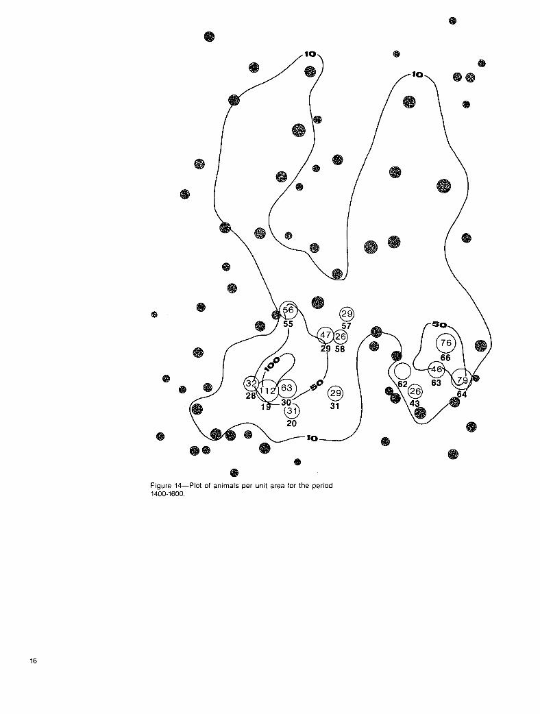
We anticipated a difference in animal activity corresponding to environmental changes during the day. Plots of the animals per unit areas for three periods--0800-1000, 1000-1400, and 1400-1600 hours (figs. 12 to 14)--suggested some progression of animal activity farther from the river during the 1000-1400 period. Deer were most active around cells 97 and 98 at this time. Throughout these periods animals

14

,o ; o o , ° ® /

\ ® O

® ° O ~ ~ O / ~

• o O ~ so

Figure 13--Plot of animals per unit area for the period 1000-1400.

remained concentrated in the main stream channel and around the 61-67 cell loca- tions. Both time-lapse photography and direct observations confirmed that some deer moved away from the river to feed on the upper benches from 1000 to 1400 hours and moved back down during the 1400-1600 time period. These movements occurred during periods of mild weather and little or no snow. Downward move- ment of deer generally corresponded to approximately the last hour of daylight suf- ficient to activate cameras, approximately 1500 to 1600 hours.

15

®

0

0

0

@

0

0 0

Q

0

0

@ @

0 @ 0

® \ o 0

@

0

® ® V ~ o

0

0

0

0

® @

)

20

®® 0 0

0 Figure 14--Plot of animals per unit area for the period 1400-1600.

@ 31

0

@ 57

0

®

63

0

~4

@

@

16

Animals per unit area.--Although occupancy of the study site did not vary ap- preciably between time periods over the years, response of the animals to the changing weather conditions during these periods probably did. Analysis-stepwise regressions of deer against the several site and environmental factors were selected to evaluate this response. The dependent variable deer was composed of animals per unit area for each cell observed. Each observation became a case for analysis. All the current attributes about cell condition at that time (both the static and dynamic variables) were the independent variables. Analyses were for:

A. All years, December-March 1. All times of observation (daylight) 2. 0800-1600 3. 0800-1000 4. 1000-1400 5. 1400-1600

B. All years, January and February combined Time periods as above.

Table 1 summarizes the information generated. Table 1 indicates multiple R 2 for the final equation for each analysis, order of inclusion in the equation and simple cor- relation r for first entry variable. Final equations for all analyses have a significance of p<0.001 and an entry level significance for variables in most cases of p<0.001 and only three variables as low as p=0.005. Only the variables that contributed to >1 percent of variance explained are included in table 1.

Table 1--Summary of stepwise regression of animals per unit of area (depend- ent variable, y) and celt variables

__l~dependent var labJg~ . . . .

E 8 8 4- u~ O

o~ ~ ~ o > ~ ~ o-" ~> ~

o

Months ~ o o ~ o o c c = ::,. -- -- First and hours Analys is R 2 >m ~ ~ ~: ~ ~ z~ -~ ~ ~ ~ ~ Cases v a r i a b l e r

- E n t r y o r d @ r , , i n t g rearesslon - -

December-

M a r c h :

Day l igh t I 0.099 2 3 1 5,717 -0.206 0800-1600 2 .093 2 3 I 2,753 -.186 0800-1000 3 .110 3 2 I 920 -.226 1000-1400 4 .396 2 1 3 7 5 4 6 1,047 .167 1400-1600 5 .159 2 3 4 5 I 786 -.233

January- February:

Day l lgh t 6 .093 1 2,689 -.211 0800-1600 7 .089 1 2,048 -.201 0800-1000 8 .106 2 3 1 668 - .103 1000-1400 9 .139 2 5 4 3 1 802 - .183 1400-1600 10 .119 3 2 1 578 - .249

17

Although we saw no major differences in the graphical analysis of number of animals in the several time periods, we speculated that there might be some differences in their relationship to local environments at certain daytimes. When data were sum- marized over longer periods of the day (analyses 1, 2, 6, and 7 of table 1), no in- fluence of any of the dynamic variables (weather) was observed in the regression equations. Best predictors during these periods were static elements, notably the YDIR variable; essentially elevation or distance from the river.

For shorter time periods, all regressions still showed the static variables dominating the regression equations, YDIR being selected as best predictor in most instances. The 1000-1400 hour regression analysis (4) is notably different in both R 2 and the selection of independent variables in the final equation. In this analysis the dynamic variables of average wind, miles accumulated in the 0 to 5 m/h speed class, and precipitation type accounted for a measurable amount of the variation in animal numbers. Windspeed alone accounted for a 17-percent increase in R 2. For this time period, animal occupancy was correlated, at least in part, to the meteorological phenomena on the site. For analysis 5, period 1400-1600 hours, cloud cover and time of measurable wind (WT) were included in the regression. For the January- February analyses during the midday and afternoon, some slight influence of weather was noted.

Generally, however, static site elements--YDIR (elevation and distance from the river), slope class, aspect, and vegetation type--accounted for most of the variation in animal numbers. Weather elements were relatively ineffective predictors of ani- mals observed per unit area.

For the data that describe cells within the study area, we might expect a degree of correlation between some of the "independent" variables. A data reduction proce- dure (factor analysis) (Kim 1975) is available that rearranges the data into a smaller set of components or factors. This analysis showed deer correlated strongly within only one factor. The strongest correlation of deer to any of the variables in this fac- tor was with XDIR with an r of 0.467. As in the regression analysis above, static variables were the best predictors of animals per unit area.

Animals per celh--We have described a series of analyses designed to relate the independent static and dynamic variables for the study area to the prediction of animals per unit area. For each cell, a subset of data describes the environmental condition relative to individual cell occupancy. An analysis could be performed for each cell based on these data. We have examined this information from only six cells selected on the basis of maximum cell usage and location: cells 29, 30, 66, 78, 85, and 95. Only dynamic variables are considered; cell constants are not iden- tified.

Table 2 presents the results of the stepwise regression analysis for each of these cells with the included variables each accounting for more than 1 percent of the variance. The entry sequence for each variable in the final equation is shown. Sim- ple r for the first entry variable and R 2 for the final regression equation are in- dicated. Note the differences in the number of animals observed, ranging from

18

Table 2--Summary of stepwise regression of deer per individual cell (deer per unit of area = dependent variable, y)

Independent v a r i a b l e s

t-

O~

L L i , = ~ Average values for

> o. 0 I 0 ~ ~ - > o • o o -- ~ ~ ~ selected varlables

E 0 0 0 c c r- E c F I rst Cell R 2 ~ u~ u~ o ~" ~ ~ ~- ~ variable r Deer Snow Temperature

Entry o rder IntQ regre}.,%lpD JZLches .~

29 0.076 2 1 -0.187 3.56 10.5 23.9 30 .296 1 2 .450 3.27 9.5 26.8 66 .090 2 1 3 - .164 4.53 7.1 29.8 78 .066 1 - .179 6.43 4.3 31.8 85 .118 3 1 2 4 - .259 13.66 4.3 33.4 95 .351 3 I 4 5 2 -.330 16.89 1.5 36.7

Discussion and Conclusions

3.27 animals/observation in cell 30 to 16.89 in cell 95. Except for cells 29 and 30, snow depth is the controlling variable; as snow depth increases, animal occupancy in general decreases. Cell 29 is notably different in its selected variables. The first entry variable is temperature with a negative coefficient. This indicates for this cell (and possibl~/for others in the valley bottoms) that animal occupancy increases with decreasing temperature. Temperature measurements in this cell on the aver- age were 23.9 °F (-4.7 °C) compared with an average of 36.7 °F (+2.6 °C) in cell 95 during animal occupancy. Snow depth differed for these cells from an average of about 10 inches (25 cm) in cell 29 to about 1.5 inches (4 cm) in cell 95 during animal occupancy. Multiple regressions are significant (p<O.O02 except p<O.01 for cell 66).

Based on the analysis of animal activity and weather events that were observed during the 4 years of this study, these conclusions were drawn about weather in the study area and the interaction of animals and site.

1. Weather data showed that winters were relatively mild compared with the pro- tracted periods of extremely cold weather observed in the recent past.

2. Topography significantly modified wind patterns and chill factor, the wind-and- temperature-dependent environmental variable. Slight changes in position within the area can rapidly affect exposure of an animal. Temperature appears much more conservative than wind as is evidenced by small departures from station 2. Exceptions occurred when cold air drainage into the valley bottoms increased temperature gradients.

19

3. Patterns of animals per unit area showed that the animals have an affinity for certain locations.

4. No major differences were observed in animal occupancy of the study area dur- ing the daytime periods. Maps of animals per unit area for various time periods showed only slight variation. Two major centers of animal concentration were observed: in the major stream channel and in a shallow headwater basin of a secondary stream. No correlation of deer per unit area and time was found.

. The regression model showed animal per unit area related differently to static and dynamic variables during the time periods selected. Static, site-dependent variables, such as cell coordinates, aspect, and slope, were the best predictors of animals per unit area. Of these, YDIR--a variable related to cell placement, approximately equal to the distance from the main river valley--was the most consistently chosen variable in the stepwise regression equations. In the anal- ysis for 1000-1400 hours, some dynamic weather variables were included in the final equation to raise the multiple R 2 to 0.396.

. Factor analysis selected four factors that represented a majority of the variability in the data set. Deer, the variable of interest, was found on only one factor primarily related to static descriptors of the site.

7. Animals per cell were examined for only 6 of the possible 89 cells observed to have deer. The weather variable snow depth was the best predictor of animals per cell for most of the selected examples. Animals per cell decreased as snow depth increased. Two cells within the main canyon were observed to have a dif- ferent set of predictive variables. One cell, 29, showed a negative correlation to temperature; that is, as temperature decreased, animals per cell increased. Other cells in the upper portion of the area all had positive correlations to temperature--cells filled as temperature increased. Animals appeared to be sen- sitive to the differences in local conditions within and between the cells.

These differences in animals per cell as related to environmental condition offer some support to the visual perception that animals moved toward the upper cells of the study area as daytime progressed (warmer temperatures) and concentrated at the lower elevations during conditions of deeper or crusted snow.

Our ability to predict animals per unit area on the study area or by implication on the more general winter range was generally poor. The single best predictor, YDIR, indicated that animals were most likely to be concentrated on the lower segments of the study area. Mapping of animal distribution showed a habitual or preferential selection of several groups of sites concentrated in the main valley bottom or in shallow headwater areas. Although some combinations of dynamic environmental factors, especially during the midday hours, influenced a movement into the upper portions of the study area, animals continued to be concentrated in these selected locations. Animals per cell showed that there was a predictable response on a cell- by-cell basis to environmental factors, but in general these factors did not modify the basic animal distributions over the area.

20

Two options for enhancing carrying capacity of these winter ranges appear feasi- ble: (1) to improve the forage and protection in areas where animals are known to congregate and (2) to modify locations nearest to these areas to improve habitat and widen the zone of expected concentrated use. A third option that would at- tempt to further disperse the animals to the main body of the study area would be inconsistent with the observed usage of the area. Major changes in site and browse would have to be made to radically alter animals' preferences regarding these widespread sites.

Option 1 seems most feasible except that it further concentrates the animals in the sites now overused. Option 2 has more potential for dispersing use to a larger area. Forage improvement through seeding with standard or improved varieties of shrubs and grasses or management of environmental factors, such as snow depth, through snow fencing or selection of vegetation heights is possible.

Unfortunately, many of the most desirable sites for deer have poor vegetation potential because of overuse and decreased soil fertility. Only through a concen- trated effort will long-term improvements be made. This effort must include careful manipulation of livestock and a stable deer herd, carefully balanced with the food supply, to prevent serious reversals in expensive habitat improvements.

21

References Connolly, G.E. 7. Limiting factors and population regulation. In: Mule and black- tailed deer of North America. Lincoln, NE: University of Nebraska Press; 1981: 245-285.

Edgerton, P.J.; Geist, J.M.; Williams, W.G. Survival and growth of Apache-plume, Stansbury cliffrose, and selected sources of antelope bitterbrush in northeastern Oregon. In: Proceedings--research and management of bitterbrush and cliffrose in western North America. Gen. Tech. Rep. INT-152. Ogden, UT: U.S. Department of Agriculture, Forest Service, Intermountain Forest and Range Experiment Sta- tion; 1983: 45-54.

Fowler, W.B. Versatile wind analyzer for long unattended runs using C-MOS. Jour- nal of Physics E. Scientific Instrumentation. 8: 713-714; 1975.

Fowler, W.B. United States patent, 4,011,752. March 15, 1977.

Garrison, G.A.; Skovlin, J.M.; Poulton, C.E.; Winward, A.H. Northwest plant names and symbols for ecosystem inventory and analysis, 4th edition. Gen. Tech. Rep. PNW-46. Portland, OR: U.S. Department of Agriculture, Forest Service, Pa- cific Northwest Forest and Range Experiment Station; 1976. 263 p.

Geist, J.M.; Edgerton, P.J. Performance tests of fourwing saltbush transplants in eastern Oregon. In: Proceedings--symposium on the biology of Atrip/ex and related chenopods. Gen. Tech. Rep. INT-172. Ogden, UT: U.S. Department of Agriculture, Forest Service, Intermountain Forest and Range Experiment Station; 1984: 244-250.

Hilken, T.O. Food habits and diet quality of deer and cattle and herbage produc- tion of a sagebrush grassland and range. Corvallis, OR: Oregon State University; 1983. M.S. thesis.

Ingles, L.G. Mammals of the Pacific States: California, Oregon and Washington. Stanford, CA: Stanford University Press; 1965.

Kim, J.O. 24. Factor analysis. In: Statistical package for the social sciences. 2d ed. New York, NY: McGraw-Hill Book Company; 1975: 468-514.

Munn, R.E. Biometeorological methods. New York, NY: Academic Press, Inc.; 1970.

Oliver, J.E. Climate and man's environment. New York, NY: John Wiley and Sons, Inc.; 1973.

22

Appendix

Chronology of Average Daily Air Temperature, Winter 1976-79

Chronology of Average Daily Windspeed, Winter 1976-79

Chill factor was computed in metric units per general use; therefore, all temper- ature and wind measurements (and snow depth) are also shown in metric units.

G"

_.= Q) O .

E I - -

G o v Q)

e~ O .

E I - -

15 11 7 3 -1 -5 -9

-13 -17 -21 -2~

15 11 7 3 -1 -5 -9

-13 -17 -21 -2~

1976 23 18

I L J

Jan--,,--. --,,-- F e b ~ ~ M a r

G 4) ,-I

4) O . E

I - -

A oo

-,[

Q) O .

E 1 9 7 7 - 7 8

11 14 t i i i i

Dec----m-- -,I---Jan---=-- --,,l-Feb-~-..-~--Mar

15 11 7 3

-1 -5 -9

-13 -17 -21 9 29 -25 ' ' I I r

Dec------ - - ,m- -Jan~ --,i-Feb-i,,,-- --==-----Mar

15

7 3 -1 -5 -9

-13 -17

-21 15 . 21 i i i i i

-25 Dec---~-- .,-,l--Jan----l-- .,,l--Feb-D,. -, i --Mar

4.0 3.6 3.2 2.8 1 9 7 6 2.4 ~ ~ 2.0 1 . 6

1.2 .8

.4 18 0 i , ~ , ,

Jan--.,,.-I-.--Feb---.---I..,.- Mar

E "O 4)

(#) "O c

4.0 3.6 3.2 2.8 2.4 2.0 1.6 1.2 .8 .4 0

~ / ~ ~ 9 \1 , V V , ' 29 , J

D e c - ~ - . --..--Jan --,,-- I--.,-Feb----- " ~ - - ' - - - M a r

"O Q)

{::

4.0 3.6 3.2 2.8 2.4 2.0 1.6 1.2

.8 .4 0

1977-78

11 i J

D e c ~ ] , - . l . . - - j a n - - - - ~ . .

~. 1,4 • -~- Feb--m-- I.--- Mar

4.0 3.6

-~- 3.2 2.8

~ 2.4 2.0

-~= 1.6 • - 1.2

.4

0 15

i i

1978-79

D e c - ~ - I -,,,,~ J a n - - - ~ I --.,- Feb --~- I - , ~ Mar

23

Chronology of Average Daily Chill Factor, Winter 1976-79

Chronology of Average Daily Snow Cover, Winter 1976-79

1200

11o0 1,-

10oo

E 900 800 0

700 o 600

m 500 400

,,C o 300

2OO

120o

11oo

I ooo

E 900

800

700

e,

.u ¢}

O O

O r - (/}

A

O

=. O O 3 O e-

09

23 18 J r i i

Jan----,'-" ' - - = ' - - - F e b ~ ~ M a r

1977-78

600

50O

4OO

30O 11 14

i = i , , ,

200 O e c - ~ ' i ' ~ J a n - - - ' l ' ' = - F e b - - ' . " --=--Mar

100

90

80

70

60

50

40

30

20

10

i 1976

o 2? , 1,8

Jan - - -= - ~ F e b ~ - -= l - - -Ma r

lOO I

:° ° 80 70

i

5oi 40 ~

30

20

lO o 11

Dec-~--=-- -.-.,---Jan---,.-

1977-78

A !' ..-,=-Feb.-=-- .-~-- M ar

1200

"7. 1100

~, lOOO

E 90o

o 800

v 700

600 f J

50o 400

t -

O 300

200

1200 T- 1100

e- lOOO

E 900

(~ 800

~oo

o 600

500

= 400 Z 0 300

2O0

t -

o

o

O e- Or)

i -

.u

O o

o u)

/ ~ 1976-7~j~

9 29 i = i p

D e c ~ .-.,,---Jan---e---I--e-Feb-=.-. ~ M a r

100

90

80

70

60

50

40

30

20

10

0

100

90

80

70

60

50

40

30

20

10

0

15 i

21 = i J

Dec-----,-- - e - - J a n ' - - - e - " " '=--Feb - e " - -e -Mar

Dec-~. . , -

1976-77

29 i =

-.-.,,--Jan--=-- -..e-Feb-e-- ~ M a r

1978-79

15 'i~ i i =

Dec---.- I--.,--Jan--.- ,--,=- Feb .-~- 21

-.~--Mar

24

Chronology of Average Daily Snow Depth, Winter 1976-79

0.50 0.45

~. 0.40 0.35 0.30 o.

"o 0.25 i= 0.20 o "" 0.15 o0

0.10 0.05

0

0.50 0.45

A 0.40 0.35

~. 0.30 0.25 "o

3 0.20 o

1976

Jan--~- .-,~Feb---=,-- ...-=--Mar

1977-78

0.10 0.05 1,1 , 14,

0 Dec--------=-- --.l--Jan---m-- --.m-Feb--~-- -,,.,-Mar

0.50 0.45

~" 0.40 v

o.

c

0.35 1976-77

0.30 1 0.25 0.20 0.15 / ~ 0.10 0.05 9 , 29,

Dec----a,,=- .-.=-Jan--=-- .--=-Feb--=.,,- --,=-~Mar

0.50

0.45 I ~- o40 1978-79 ~" 0.35 o. 0.30 "o 0.25

0.20 O9 0.15

0.10

0.05 15 21 0 ~

Dec ----==- . - . = - - J a n ~ -.,=--Feb--==-..-,e--Mar

25

Fowler, W.B.; Dealy, J.E. Behavior of mule deer on the Keating Winter Range. Res. Pap. PNW-RP-373. Portland, OR: U.S. Department of Agriculture, Forest Service, Pacific Northwest Research Station; 1987. 25 p.

Observations are presented from 4 years of record, 1976 to 1979, on behavior of mule deer (Odocoileus hemionus) in relation to site variables on the Keating Winter Range in northeastern Oregon. Analyses of animal use per unit area showed that the preferential selection of cells was related primarily to static site variables and secondarily to weather. The most regularly selected and strongest predictive variable was distance from the valley bottom, a variable generally associated with elevation. Only during the midafternoon hours of 1400 to 1600 did dynamic weather variables contribute substantially to the variance explained by the regression equations. For individual cells, animal use was controlled by snow depth and temperature.

Keywords: Animal behavior, winter range, deer (mule).

The Forest Service of the U.S. Department of Ag r i cu l t u re is ded ica ted to the p r inc ip le of m u l t i p l e use managemen t of the Na t i on ' s fo res t resources for sus ta ined y ie lds of wood, water , forage, w i ld l i f e , and recreat ion. Through fo res t r y research, coopera t i on w i th the Sta tes and pr ivate fo res t owners , and m a n a g e m e n t of the Nat iona l Fores ts and Nat ional Grasslands, it s t r ives - - as d i rected by Congress m to prov ide i nc reas ing l y greater serv ice to a g row ing Nat ion.

The U.S. Depar tmen t of Ag r i cu l t u re is an Equal Oppor tun i ty Employer. App l i can ts for all Depar tment p rograms wi l l be g iven equal cons ide ra t i on w i t h o u t regard to age, race, co lor , sex, re l ig ion, or na t iona l or ig in .

Pacific Northwest Research Station 319 S.W. Pine St. P.O. Box 3890 Portland, Oregon 97208

+~, ~,. ~ ,': .%' ,~ :~ ,~ + • , ~. , ~% % g.~ ;+-~ ~< ~+,~

~:~! i~ i • ~< ~2:~ ~ ~:m" ~~ +~ ~'-:'-~"' +'':~!

~<~:~+,~,~ ~++ ....... :: :~i:~ ~ !_:,;,<~.~ '~k.+,<~ ~, ~ , :;~!: ~,

: ~ :: ~+~ ~++ ~ ~, ~ ~!!~ LI ~ .-L ~ ,~ ~:- ~i~<'~ ~, :.+'~<ii

~.~ ~ : ~. ~.: +.+r'~ ~

:'.~ii~% _~i,~ ~ i', ~~ <, ~<-'[! '

i:~,.:i: <::,%<.:' k: g%~

.... -,+.~m £ + ++:~: . ~,

!~..<4 • + ~ .c~: +.,

9 : ~,'G ~' ':-~j~< J'{: %:j!:~_%

~i{ii:~<~£i i {:}! <)"<, b+: i ;r. ~ +-, }L:L: ",~"

~ ~n ~

.... ~+ ,+- ............ ": '~:':~:+ ' + ' : ~ < ' : : Z< ",~ff+ +,~. 7 : - , f ~. ; 4~,% .',? (_ . . . . ,:+ ] ~, .~- ; . . . : :.~