Beginning Trajectory Analysis with Bio3D

Lars Skjaerven, Xin-Qiu Yao and Barry J. GrantUniversity of Michigan, Ann Arbor

November 13, 2013

1 Background

Bio3D1 is an R package that provides interactive tools for the analysis of bimolecular structure, sequenceand simulation data. The aim of this document, termed a vignette2 in R parlance, is to provide a brieftask-oriented introduction to basic molecular dynamics trajectory analysis with the Bio3D R package (Grantet al., 2006).

Requirements: Detailed instructions for obtaining and installing the Bio3D package on various platformscan be found in the Installing Bio3D vignette available both on-line and from within the Bio3D package. Tosee available vignettes use the command:

vignette(package = "bio3d")

2 Getting Started

Start R, load the Bio3D package and use the command demo("md") to get a quick feel for some of the tasksthat we will be introducing in the following sections.

library(bio3d)

demo("md")

Side-note: Note that you will be prompted to hit the RETURN key at each step of the demo as this will allowyou to see the particular functions being called. Also note that detailed documentation and example code foreach function can be accessed via the help() and example() commands (e.g. help(read.pdb)). You canalso copy and paste any of the example code from the documentation of a particular function, or indeed thisvignette, directly into your R session to see how things work. You can also find this documentation online.

2.1 Reading Example Trajectory Data

A number of example data sets are shipped with the Bio3D package. The main purpose of including thisdata is to allow users to more quickly appreciate the capabilities of various Bio3D functions that wouldotherwise require potentially time consuming data generation. In the examples below we will input, processand analyze a molecular dynamics trajectory of Human Immunodeficiency Virus aspartic protease (HIVpr).This trajectory is stored in CHARMM/NAMD DCD format and has had all solvent and non C-alpha proteinatoms excluded to reduce overall file size.

1The latest version of the package, full documentation and further vignettes (including detailed installation instructions) canbe obtained from the main Bio3D website: http://thegrantlab.org/bio3d/

2This vignette contains executable examples, see help(vignette) for further details.

1

The code snippet below sets the file paths for the example HIVpr starting structure (pdbfile) and trajectorydata (dcdfile).

dcdfile <- system.file("examples/hivp.dcd", package = "bio3d")

pdbfile <- system.file("examples/hivp.pdb", package = "bio3d")

Side-note: Note that in the above example the system.file() command returns a character string cor-responding to the file name of a PDB structure included with the Bio3D package. This is required as usersmay install the package in different locations. When using your own input files the system.file() commandwill not be required, for example

mydcdfile <- "/path/to/my/data/myfile.dcd"

dcd <- read.dcd(dcdfile)

pdb <- read.pdb(pdbfile)

The read.dcd() and read.pdb() commands processes the input files and returns their output to thenew objects dcd and pdb. We can check the basic structure of these objects with the following commands:

print(pdb)

##

## Call: read.pdb(file = pdbfile)

##

## Atom Count: 198

##

## Total ATOMs#: 198

## Protein ATOMs#: 198 ( Calpha ATOMs#: 198 )

## Non-protein ATOMs#: 0 ( residues: )

## Chains#: 2 ( values: A B )

##

## Total HETATOMs: 0

## Residues HETATOMs#: 0 ( residues: )

## Chains#: 0 ( values: )

##

## Sequence:

## PQITLWQRPLVTIKIGGQLKEALLDTGADDTVLEEMSLPGRWKPKMIGGIGGFIKVRQYD

## QILIEICGHKAIGTVLVGPTPVNIIGRNLLTQIGCTLNFPQITLWQRPLVTIKIGGQLKE

## ALLDTGADDTVLEEMSLPGRWKPKMIGGIGGFIKVRQYDQILIEICGHKAIGTVLVGPTP

## VNIIGRNLLTQIGCTLNF

##

## + attr: atom, het, helix, sheet, seqres,

## xyz, xyz.models, calpha, call

length(pdb$xyz)

## [1] 594

dim(dcd)

## [1] 351 594

Note that the output of the dim() function is telling us that we have 351 trajectory frames (or rows inour dcd matrix) and 594 coordinates (or x, y and z columns).

2

Question: How many atoms are in the trajectory and PDB files?

Question: How would you extract the amino acid sequence of the HIVpr system in 1-letter and 3-letterforms? HINT: try help.search("PDB sequence") for a Bio3D function that might help you.

Side-note: Note that typically one works with trajectory files that contain all protein atoms, or at the veryleast all backbone atoms. Solvent however can often be excluded prior to Bio3D input - it just depends uponyour particular analysis questions. For example, we are not able to analyze Hydrogen bonding patterns ordetails of water occupancy with the currently inputed data.

3 Trajectory Frame Superposition

In this simple example we select all C-alpha atoms for trajectory frame superposition.

ca.inds <- atom.select(pdb, elety = "CA")

##

## Build selection from input components

##

## segid chain resno resid eleno elety

## Stest "" "" "" "" "" "CA"

## Natom "198" "198" "198" "198" "198" "198"

## * Selected a total of: 198 intersecting atoms *

The returned ca.inds object is a list containing atom and xyz numeric indices that we can now use tosuperpose all frames of the trajectory on the selected indices (in this case corresponding to all alpha Carbonatoms). For this we will with the fit.xyz() function.

xyz <- fit.xyz(fixed = pdb$xyz, mobile = dcd, fixed.inds = ca.inds$xyz, mobile.inds = ca.inds$xyz)

The above command performs the actual superposition and stores the new coordinates in the matrixobject xyz. Note that the dimensions (i.e. number of rows and columns, which correspond to frames andcoordinates respectively) of xyz match those of the input trajectory:

dim(xyz) == dim(dcd)

## [1] TRUE TRUE

Question: How would you fit trajectory frames on the Calpha atoms of residues 24 to 27 and 85 to 90 inboth chains? HINT: See the example section of help(atom.select).

Question: Would you expect the alternate fitting suggested above to alter your later results? HINT: Youcan come back to this question later after going through the other sections.

Side-note: A simple way to obtain the average structure from your fitted trajectory is to use the followingcommand apply(xyz,2,mean).

4 Root Mean Square Deviation (RMSD)

RMSD is a standard measure of structural distance between coordinate sets and is implemented in the Bio3Dfunction rmsd().

3

rd <- rmsd(xyz[1, ca.inds$xyz], xyz[, ca.inds$xyz])

plot(rd, typ = "l", ylab = "RMSD", xlab = "Frame No.")

points(lowess(rd), typ = "l", col = "red", lty = 2, lwd = 2)

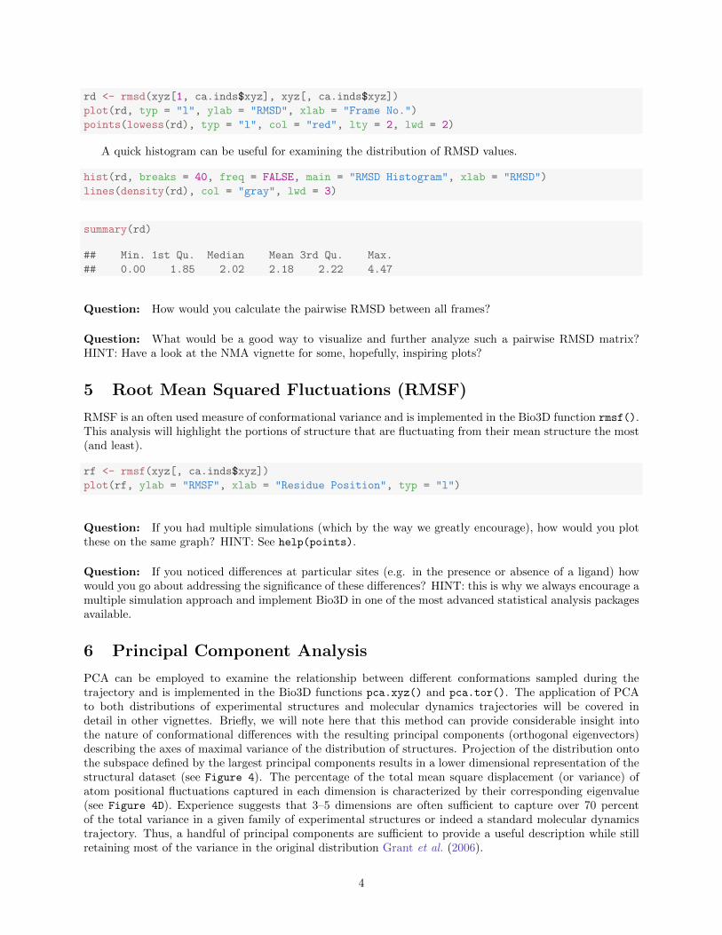
A quick histogram can be useful for examining the distribution of RMSD values.

hist(rd, breaks = 40, freq = FALSE, main = "RMSD Histogram", xlab = "RMSD")

lines(density(rd), col = "gray", lwd = 3)

summary(rd)

## Min. 1st Qu. Median Mean 3rd Qu. Max.

## 0.00 1.85 2.02 2.18 2.22 4.47

Question: How would you calculate the pairwise RMSD between all frames?

Question: What would be a good way to visualize and further analyze such a pairwise RMSD matrix?HINT: Have a look at the NMA vignette for some, hopefully, inspiring plots?

5 Root Mean Squared Fluctuations (RMSF)

RMSF is an often used measure of conformational variance and is implemented in the Bio3D function rmsf().This analysis will highlight the portions of structure that are fluctuating from their mean structure the most(and least).

rf <- rmsf(xyz[, ca.inds$xyz])

plot(rf, ylab = "RMSF", xlab = "Residue Position", typ = "l")

Question: If you had multiple simulations (which by the way we greatly encourage), how would you plotthese on the same graph? HINT: See help(points).

Question: If you noticed differences at particular sites (e.g. in the presence or absence of a ligand) howwould you go about addressing the significance of these differences? HINT: this is why we always encourage amultiple simulation approach and implement Bio3D in one of the most advanced statistical analysis packagesavailable.

6 Principal Component Analysis

PCA can be employed to examine the relationship between different conformations sampled during thetrajectory and is implemented in the Bio3D functions pca.xyz() and pca.tor(). The application of PCAto both distributions of experimental structures and molecular dynamics trajectories will be covered indetail in other vignettes. Briefly, we will note here that this method can provide considerable insight intothe nature of conformational differences with the resulting principal components (orthogonal eigenvectors)describing the axes of maximal variance of the distribution of structures. Projection of the distribution ontothe subspace defined by the largest principal components results in a lower dimensional representation of thestructural dataset (see Figure 4). The percentage of the total mean square displacement (or variance) ofatom positional fluctuations captured in each dimension is characterized by their corresponding eigenvalue(see Figure 4D). Experience suggests that 3–5 dimensions are often sufficient to capture over 70 percentof the total variance in a given family of experimental structures or indeed a standard molecular dynamicstrajectory. Thus, a handful of principal components are sufficient to provide a useful description while stillretaining most of the variance in the original distribution Grant et al. (2006).

4

0 50 100 150 200 250 300 350

01

23

4

Frame No.

RM

SD

Figure 1: Simple time series of RMSD from the initial structure (note periodic jumps that we will later seecorrespond to transient openings of the flap regions of HIVpr)

5

RMSD Histogram

RMSD

Den

sity

0 1 2 3 4

0.0

0.5

1.0

1.5

Figure 2: Note the spread of RMSD values and that the majority of sampled conformations are around 2Angstroms from the starting structure

6

0 50 100 150 200

1.0

1.5

2.0

2.5

3.0

3.5

Residue Position

RM

SF

Figure 3: Residue-wise RMSF indicates regions of high mobility

7

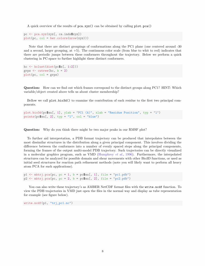
A quick overview of the results of pca.xyz() can be obtained by calling plot.pca()

pc <- pca.xyz(xyz[, ca.inds$xyz])

plot(pc, col = bwr.colors(nrow(xyz)))

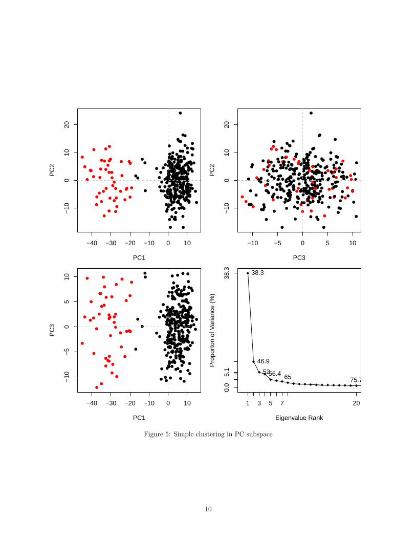
Note that there are distinct groupings of conformations along the PC1 plane (one centered around -30and a second, larger grouping, at +5). The continuous color scale (from blue to whit to red) indicates thatthere are periodic jumps between these conformers throughout the trajectory. Below we perform a quickclustering in PC-space to further highlight these distinct conformers.

hc <- hclust(dist(pc$z[, 1:2]))

grps <- cutree(hc, k = 2)

plot(pc, col = grps)

Question: How can we find out which frames correspond to the distinct groups along PC1? HINT: Whichvariable/object created above tells us about cluster membership?

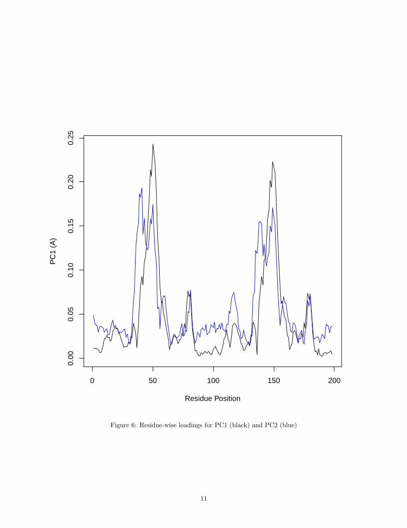
Bellow we call plot.bio3d() to examine the contribution of each residue to the first two principal com-ponents.

plot.bio3d(pc$au[, 1], ylab = "PC1 (A)", xlab = "Residue Position", typ = "l")

points(pc$au[, 2], typ = "l", col = "blue")

Question: Why do you think there might be two major peaks in our RMSF plot?

To further aid interpretation, a PDB format trajectory can be produced that interpolates between themost dissimilar structures in the distribution along a given principal component. This involves dividing thedifference between the conformers into a number of evenly spaced steps along the principal components,forming the frames of the output multi-model PDB trajectory. Such trajectories can be directly visualizedin a molecular graphics program, such as VMD (Humphrey et al., 1996). Furthermore, the interpolatedstructures can be analyzed for possible domain and shear movements with other Bio3D functions, or used asinitial seed structures for reaction path refinement methods (note you will likely want to perform all heavyatom PCA for such applications).

p1 <- mktrj.pca(pc, pc = 1, b = pc$au[, 1], file = "pc1.pdb")

p2 <- mktrj.pca(pc, pc = 2, b = pc$au[, 2], file = "pc2.pdb")

You can also write these trajectory’s as AMBER NetCDF format files with the write.ncdf function. Toview the PDB trajectories in VMD just open the files in the normal way and display as tube representationfor example (see figure below).

write.ncdf(p1, "trj_pc1.nc")

8

●

●

●

●

●

●

●

●

●

●

●

●

●

●●

●

●●

●●

●

● ●

● ●

●

●● ●

●

●

●

●●

●

●

●

●

●

●

●

●

●●

●

●

●

●●

●

●

●

●

●●

●

●

●●

●

●

● ●●

●

●

●

●

●

●

●

●

●

●

●

●

●●●

●

●

●●

●

●●

●

●

●

●

●

●

●

●

●

●

●

●

●

●

●

● ●

●

●

●●

●

●

●

●

●

●

●

●

●

●

●

●

●

●

●

●●

●

●

●

●

●

●

●

●

●

●● ●●

● ●

●

●●●●

●

●

●

●

●

●

●

●

●

●

●

●●

●

●

●●

●

●

●

●

●

●●●

●

●

●●●

●

● ●●

●

●

● ●

●

●

●

●

●●

●

●

●

●

●

●

●

●

●

●

●

●

●

●●

●

●

●

●●

●

●

●

●

●

●●

●

●

●

●

●

●

●

●●

●

●

●

●

●

●●

●

●

●

●

●

●

●

●

●

●

●

●●

●

●

●

●

●

●

●

●

●

●

●●

●

●

●

●

●

●●●

●

●

●

●

●

● ●

●

●

●

●

●

●

●

●

●

●

●

●●●

● ●

●

●

●

●

●●

●

●●

●

●

●●

●

●

●

●

●

●

●

●

●

●

●

●

●

●

●

●

●

●●●

●

●●

●

● ●●

●

●

●●

●

●

●

●

●●

●●

●

●

●

●

●

●

●●

●

●

●

●

−40 −30 −20 −10 0 10

−10

010

20

PC1

PC

2

●

●

●

●

●

●

●

●

●

●

●

●

●

●●

●

●●

●●

●

●●

●●

●

●● ●

●

●

●

●●

●

●

●

●

●

●

●

●

●●

●

●

●

●●

●

●

●

●

●●

●

●

●●

●

●

●●●

●

●

●

●

●

●

●

●

●

●

●

●

●●●

●

●

●●

●

●●

●

●

●

●

●

●

●

●

●

●

●

●

●

●

●

●●

●

●

●●

●

●

●

●

●

●

●

●

●

●

●

●

●

●

●

●●

●

●

●

●

●

●

●

●

●

● ●●●

●●

●

●● ●●

●

●

●

●

●

●

●

●

●

●

●

●●

●

●

●●

●

●

●

●

●

●● ●

●

●

●●●

●

●●●

●

●

● ●

●

●

●

●

● ●

●

●

●

●

●

●

●

●

●

●

●

●

●

● ●

●

●

●

●●

●

●

●

●

●

● ●

●

●

●

●

●

●

●

● ●

●

●

●

●

●

●●

●

●

●

●

●

●

●

●

●

●

●

●●

●

●

●

●

●

●

●

●

●

●

●●

●

●

●

●

●

●● ●

●

●

●

●

●

● ●

●

●

●

●

●

●

●

●

●

●

●

●●●

●●

●

●

●

●

●●

●

●●

●

●

●●

●

●

●

●

●

●

●

●

●

●

●

●

●

●

●

●

●

●●●

●

●●

●

● ●●

●

●

●●

●

●

●

●

●●

●●

●

●

●

●

●

●

●●

●

●

●

●

−10 −5 0 5 10

−10

010

20

PC3

PC

2

●

●

●

●

●

●

●

●

●

●

●

●

●

●

●●

●

●●

●

●

●

●

●

●●

●

●

●

●

●

●

●

●

●

●

●

●

●

●

●

●

●●

●●●

●

●

●●

●

●

●

●

●

●●

●

●

●

●●

●

●

●

●

●

●

●

●

●

●●

●

●

●

●

●

●

●

●

●

●

●

●●●

●

●

●

●

●

●

●

●

●

●

●●

●●●

●

●

●

●

●

●

●

●

● ●●

●

●

●

●

●

●

●

●

●

●

●

●

●

●

●

●

●

●

●

●

●

●

●●

●

●

●

●

●●

●●

●●

●

●

●

●

●

●

●

●

●

●

●

●

●

●

●●

●

●

●

●

●

●

●

●

●

●

●

●

●

●

●

●●

●●

●●

●

●

●

●●●

●●

●

●

●

●

●

●

●

●

●

●

●●

●

●

●

●

●●

●

●

●

●

●

●

●

●

●

●

●

●

●

●

●

●

●●

●

●

●

●

●

●

●

●

●●●

●●

●

●

●

●

●

●

●●

●

●

●

●

●

●

●

●

●

●

●

●

●

● ●

●

●

●

●

●

●

●

●

●

●●

●

●

●

●

●

●

●

●

●

●

●

●

●

●

●

●

●

●

●

●

●

●

●

●

●

●

●

●

●

●

●●

●

●

●

●

●

●●

●

●

●●

●

●●

●

●

●

●

●

●

●

●

●

●

●

●

●

●

●

●

●

●

●

●

●

●

●

●

●

●

●●

●

−40 −30 −20 −10 0 10

−10

−5

05

10

PC1

PC

3

1 3 5 7 20

0.0

5.1

38.3 38.3

46.9

5256.4 65 75.7

Eigenvalue Rank

Pro

port

on o

f Var

ianc

e (%

)

Figure 4: PCA results for our HIVpr trajectory with instantaneous conformations (i.e. trajectory frames)colored from blue to red in order of time

9

●

●

●

●

●

●

●

●

●

●

●

●

●

●●

●

●●

●●

●

● ●

● ●

●

●● ●

●

●

●

●●

●

●

●

●

●

●

●

●

●●

●

●

●

●●

●

●

●

●

●●

●

●

●●

●

●

● ●●

●

●

●

●

●

●

●

●

●

●

●

●

●●●

●

●

●●

●

●●

●

●

●

●

●

●

●

●

●

●

●

●

●

●

●

● ●

●

●

●●

●

●

●

●

●

●

●

●

●

●

●

●

●

●

●

●●

●

●

●

●

●

●

●

●

●

●● ●●

● ●

●

●●●●

●

●

●

●

●

●

●

●

●

●

●

●●

●

●

●●

●

●

●

●

●

●●●

●

●

●●●

●

● ●●

●

●

● ●

●

●

●

●

●●

●

●

●

●

●

●

●

●

●

●

●

●

●

●●

●

●

●

●●

●

●

●

●

●

●●

●

●

●

●

●

●

●

●●

●

●

●

●

●

●●

●

●

●

●

●

●

●

●

●

●

●

●●

●

●

●

●

●

●

●

●

●

●

●●

●

●

●

●

●

●●●

●

●

●

●

●

● ●

●

●

●

●

●

●

●

●

●

●

●

●●●

● ●

●

●

●

●

●●

●

●●

●

●

●●

●

●

●

●

●

●

●

●

●

●

●

●

●

●

●

●

●

●●●

●

●●

●

● ●●

●

●

●●

●

●

●

●

●●

●●

●

●

●

●

●

●

●●

●

●

●

●

−40 −30 −20 −10 0 10

−10

010

20

PC1

PC

2

●

●

●

●

●

●

●

●

●

●

●

●

●

●●

●

●●

●●

●

●●

●●

●

●● ●

●

●

●

●●

●

●

●

●

●

●

●

●

●●

●

●

●

●●

●

●

●

●

●●

●

●

●●

●

●

●●●

●

●

●

●

●

●

●

●

●

●

●

●

●●●

●

●

●●

●

●●

●

●

●

●

●

●

●

●

●

●

●

●

●

●

●

●●

●

●

●●

●

●

●

●

●

●

●

●

●

●

●

●

●

●

●

●●

●

●

●

●

●

●

●

●

●

● ●●●

●●

●

●● ●●

●

●

●

●

●

●

●

●

●

●

●

●●

●

●

●●

●

●

●

●

●

●● ●

●

●

●●●

●

●●●

●

●

● ●

●

●

●

●

● ●

●

●

●

●

●

●

●

●

●

●

●

●

●

● ●

●

●

●

●●

●

●

●

●

●

● ●

●

●

●

●

●

●

●

● ●

●

●

●

●

●

●●

●

●

●

●

●

●

●

●

●

●

●

●●

●

●

●

●

●

●

●

●

●

●

●●

●

●

●

●

●

●● ●

●

●

●

●

●

● ●

●

●

●

●

●

●

●

●

●

●

●

●●●

●●

●

●

●

●

●●

●

●●

●

●

●●

●

●

●

●

●

●

●

●

●

●

●

●

●

●

●

●

●

●●●

●

●●

●

● ●●

●

●

●●

●

●

●

●

●●

●●

●

●

●

●

●

●

●●

●

●

●

●

−10 −5 0 5 10

−10

010

20

PC3

PC

2

●

●

●

●

●

●

●

●

●

●

●

●

●

●

●●

●

●●

●

●

●

●

●

●●

●

●

●

●

●

●

●

●

●

●

●

●

●

●

●

●

●●

●●●

●

●

●●

●

●

●

●

●

●●

●

●

●

●●

●

●

●

●

●

●

●

●

●

●●

●

●

●

●

●

●

●

●

●

●

●

●●●

●

●

●

●

●

●

●

●

●

●

●●

●●●

●

●

●

●

●

●

●

●

● ●●

●

●

●

●

●

●

●

●

●

●

●

●

●

●

●

●

●

●

●

●

●

●

●●

●

●

●

●

●●

●●

●●

●

●

●

●

●

●

●

●

●

●

●

●

●

●

●●

●

●

●

●

●

●

●

●

●

●

●

●

●

●

●

●●

●●

●●

●

●

●

●●●

●●

●

●

●

●

●

●

●

●

●

●

●●

●

●

●

●

●●

●

●

●

●

●

●

●

●

●

●

●

●

●

●

●

●

●●

●

●

●

●

●

●

●

●

●●●

●●

●

●

●

●

●

●

●●

●

●

●

●

●

●

●

●

●

●

●

●

●

● ●

●

●

●

●

●

●

●

●

●

●●

●

●

●

●

●

●

●

●

●

●

●

●

●

●

●

●

●

●

●

●

●

●

●

●

●

●

●

●

●

●

●●

●

●

●

●

●

●●

●

●

●●

●

●●

●

●

●

●

●

●

●

●

●

●

●

●

●

●

●

●

●

●

●

●

●

●

●

●

●

●

●●

●

−40 −30 −20 −10 0 10

−10

−5

05

10

PC1

PC

3

1 3 5 7 20

0.0

5.1

38.3 38.3

46.9

5256.4 65 75.7

Eigenvalue Rank

Pro

port

on o

f Var

ianc

e (%

)

Figure 5: Simple clustering in PC subspace

10

0 50 100 150 200

0.00

0.05

0.10

0.15

0.20

0.25

Residue Position

PC

1 (A

)

Figure 6: Residue-wise loadings for PC1 (black) and PC2 (blue)

11

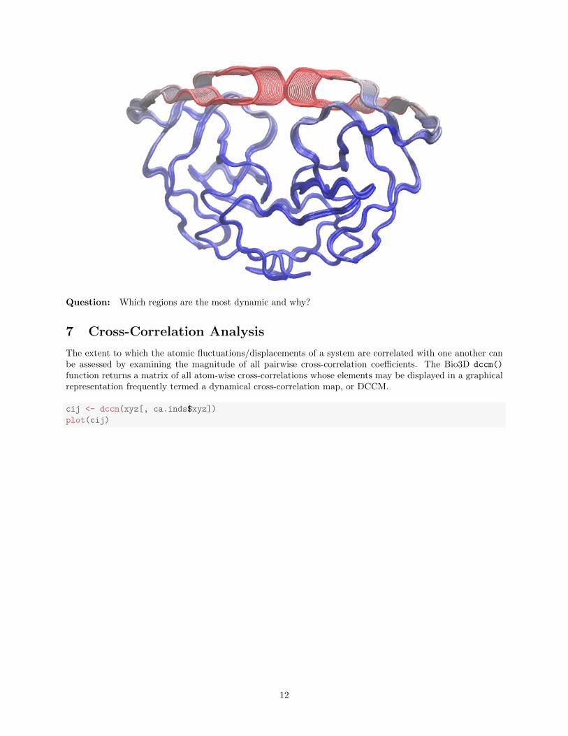
Question: Which regions are the most dynamic and why?

7 Cross-Correlation Analysis

The extent to which the atomic fluctuations/displacements of a system are correlated with one another canbe assessed by examining the magnitude of all pairwise cross-correlation coefficients. The Bio3D dccm()

function returns a matrix of all atom-wise cross-correlations whose elements may be displayed in a graphicalrepresentation frequently termed a dynamical cross-correlation map, or DCCM.

cij <- dccm(xyz[, ca.inds$xyz])

plot(cij)

12

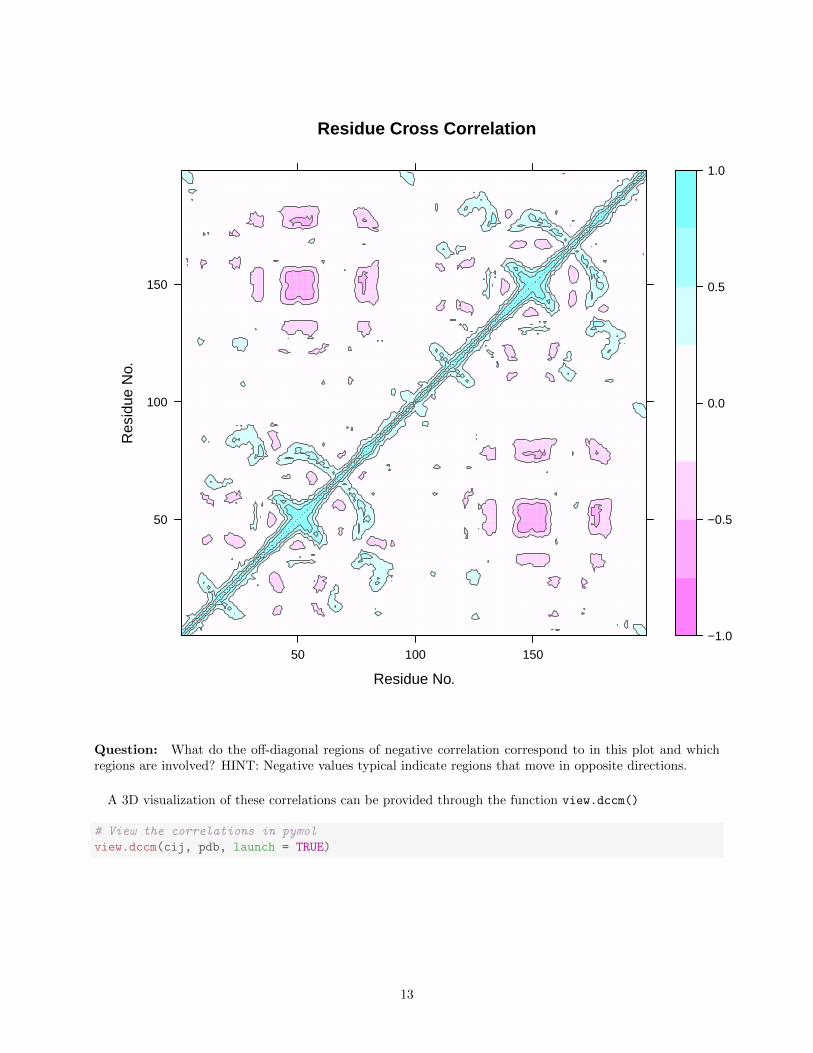
Residue Cross Correlation

Residue No.

Res

idue

No.

50

100

150

50 100 150

−1.0

−0.5

0.0

0.5

1.0

Question: What do the off-diagonal regions of negative correlation correspond to in this plot and whichregions are involved? HINT: Negative values typical indicate regions that move in opposite directions.

A 3D visualization of these correlations can be provided through the function view.dccm()

# View the correlations in pymol

view.dccm(cij, pdb, launch = TRUE)

13

See also the Enhanced Methods for Normal Mode Analysis for additional visualization examples. Alsoyou might want to checkout the Comparative Analysis of Protein Structures vignette for relating re-sults like these to available experimental data. The logical expansion of this analysis is described in theCorrelation Network Analysis vignette.

8 Where to Next

If you have read this far, congratulations! We are ready to have some fun and move to other packagevignettes that describe more interesting analysis including Correlation Network Analysis (where we will buildand dissect dynamic networks form different correlated motion data), enhanced methods for Normal ModeAnalysis (where we will explore the dynamics of large protein families and superfamilies), and advancedComparative Structure Analysis (where we will mine available experimental data and supplement it withsimulation results to map the conformational dynamics and coupled motions of proteins).

9 Document Details

This document is shipped with the Bio3D package in both Rnw and PDF formats. All code can be extractedand automatically executed to generate Figures and/or the PDF with the following commands:

knitr::knit("Bio3D_md.Rnw")

tools::texi2pdf("Bio3D_md.tex")

Information About the Current Bio3D Session

sessionInfo()

## R version 3.0.2 (2013-09-25)

## Platform: x86_64-apple-darwin10.8.0 (64-bit)

##

## locale:

## [1] en_US.UTF-8/en_US.UTF-8/en_US.UTF-8/C/en_US.UTF-8/en_US.UTF-8

14

##

## attached base packages:

## [1] grid stats graphics utils datasets grDevices methods

## [8] base

##

## other attached packages:

## [1] lattice_0.20-24 bio3d_2.0-1

##

## loaded via a namespace (and not attached):

## [1] digest_0.6.3 evaluate_0.5.1 formatR_0.9 highr_0.2.1

## [5] knitr_1.5 stringr_0.6.2 tools_3.0.2

References

Grant, B.J. and Rodrigues, A.P.D.C and Elsawy, K.M. and Mccammon, A.J. and Caves, L.S.D. (2006)Bio3d: an R package for the comparative analysis of protein structures. Bioinformatics, 22,2695–2696.

Humphrey, W., et al. (1996) VMD: visual molecular dynamics. J. Mol. Graph, 14, 33–38

15