Beer Demand
5
Economics Letters 61 (1998) 67–71 Elasticities of beer demand revisited * Craig A. Gallet , John A. List Department of Economics, University of Central Florida, P .O. Box 161400, Orlando, FL 32816-1400, USA Received 15 October 1997; accepted 25 June 1998 Abstract This paper uses U.S. aggregate beer consumption data from 1964–1992 to empirically estimate the elasticities of demand for beer. However, rather than assuming the behavioral parameters are time invariant, we estimate a gradual switching regression model that explicitly allows the elasticities to change over time. Results suggest that this more general model is warranted, as findings illustrate the importance of variable dynamics when evaluating the efficacy of proposed policy alternatives. 1998 Elsevier Science S.A. All rights reserved. Keywords: Beer demand; Gradual switching regression JEL classification: D10; C22 1. Introduction Measuring elasticities of beer demand has become commonplace since the seminal work of Niskanen (1962). This is not surprising given that beer constitutes one of the most heavily taxed goods in U.S. history. Yet it is surprising that empirical studies have largely ignored the possibility 1 that these elasticities may be heterogeneous over time. Economic theory provides numerous reasons why they may not be constant. For example, given the health risks of drinking became more apparent in the 1970s and 1980s (see, e.g., Lee and Tremblay, 1992), in light of theoretical models developed by Viscusi (1990) and Viscusi and Evans (1991), rational beer consumers should adjust their sensitivity to changes in price and income. Using aggregate beer consumption data for the U.S. over the 1964–1992 period, we relax the restriction of response homogeneity over time and allow for a gradual adjustment of the estimated elasticities. Consistent with recent developments in the beer industry, the results indicate that elasticities began to adjust in 1973 and fully adjusted by 1983. In the remainder of this note, Section 2 describes the data and econometric techniques employed. Section 3 presents empirical results and Section 4 provides concluding comments. * Corresponding author: Tel.: 11 407 8233720; e-mail: [email protected] 1 One exception is Horowitz and Horowitz (1965), who estimate the demand for beer across states using 13 regressions for the period 1949–1961. They find that elasticities change over the sample period. 0165-1765 / 98 / $ – see front matter 1998 Elsevier Science S.A. All rights reserved. PII: S0165-1765(98)00146-3
-
Upload
sneha-khurana -
Category
Documents
-
view
213 -
download
0
description
Economics and Beer Demand
Transcript of Beer Demand
Economics Letters 61 (1998) 67–71
Elasticities of beer demand revisited*Craig A. Gallet , John A. List
Department of Economics, University of Central Florida, P.O. Box 161400, Orlando, FL 32816-1400, USA
Received 15 October 1997; accepted 25 June 1998
Abstract
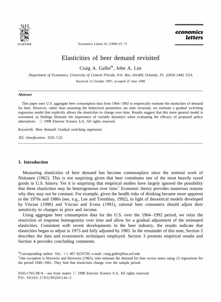
This paper uses U.S. aggregate beer consumption data from 1964–1992 to empirically estimate the elasticities of demandfor beer. However, rather than assuming the behavioral parameters are time invariant, we estimate a gradual switchingregression model that explicitly allows the elasticities to change over time. Results suggest that this more general model iswarranted, as findings illustrate the importance of variable dynamics when evaluating the efficacy of proposed policyalternatives. 1998 Elsevier Science S.A. All rights reserved.
Keywords: Beer demand; Gradual switching regression
JEL classification: D10; C22
1. Introduction
Measuring elasticities of beer demand has become commonplace since the seminal work ofNiskanen (1962). This is not surprising given that beer constitutes one of the most heavily taxedgoods in U.S. history. Yet it is surprising that empirical studies have largely ignored the possibility
1that these elasticities may be heterogeneous over time. Economic theory provides numerous reasonswhy they may not be constant. For example, given the health risks of drinking became more apparentin the 1970s and 1980s (see, e.g., Lee and Tremblay, 1992), in light of theoretical models developedby Viscusi (1990) and Viscusi and Evans (1991), rational beer consumers should adjust theirsensitivity to changes in price and income.
Using aggregate beer consumption data for the U.S. over the 1964–1992 period, we relax therestriction of response homogeneity over time and allow for a gradual adjustment of the estimatedelasticities. Consistent with recent developments in the beer industry, the results indicate thatelasticities began to adjust in 1973 and fully adjusted by 1983. In the remainder of this note, Section 2describes the data and econometric techniques employed. Section 3 presents empirical results andSection 4 provides concluding comments.
*Corresponding author: Tel.: 11 407 8233720; e-mail: [email protected] exception is Horowitz and Horowitz (1965), who estimate the demand for beer across states using 13 regressions forthe period 1949–1961. They find that elasticities change over the sample period.
0165-1765/98/$ – see front matter 1998 Elsevier Science S.A. All rights reserved.PI I : S0165-1765( 98 )00146-3

68 C.A. Gallet, J.A. List / Economics Letters 61 (1998) 67 –71
2. Empirical methodology and data description
The traditional approach to test for temporal change in equation structure is to include a dummy2variable and estimate a spline function. Such an approach assumes structural breaks are exogenously
determined and parameter adjustments are instantaneous. However, the habit formation model ofPollack and Wales (1969), which suggests that consumers may respond slowly to new information,implies a more relaxed estimation technique is warranted. Specifically, to allow for a gradual changein the demand parameters over an endogenously determined time path, we estimate the U.S. demandfor beer using a gradual switching regression model (see, e.g., Ohtani and Katayama, 1985; Ohtani etal., 1990), given by:
i
S 5 a 1O (b 1 F f )X 1 ´ t 5 1, 2,....., T (1)t i t i it t ;2
where S is the tth observation of the natural log of per capita (persons 18 and over) beert
consumption, X is the tth observation of the natural log of the ith regressor (which includes real priceit3of beer, real price of wine, and real per capita income), F is a gradual adjustment path which equalst
0 before the adjustment and 1 after the adjustment is completed, b and f are unknown parameters ofi i2 4interest, and the error term, ´ |N(0, s ). Appendix A contains a complete description of the data.t ´
We allow the coefficients to gradually change (from b to b 1f ) by permitting F to vary along ai i i t
linear transition path, given by:
*F 5 0 , for t , t , (2)t 1
* *5 a 1 a t , for t # t # t ,0 1 1 2
*5 1 , for t . t ,2
* *where t is the end-point of the first regime (estimated coefficients are b ) and t is the start-point of1 i 25 * *the second regime (estimated coefficients become b 1f ). Given values of t and t , it can be showni i 1 2
* *that for t #t#t :1 2
* * *F 5 (t 2 t ) /(t 2 t ) (3)t 1 2 1
We use a method similar to Ohtani and Katayama (1985); Ohtani et al. (1990) to obtain the start
2For example, Hamilton (1974); Bishop and Yoo (1985) use dummy variables to account for the effect of health informationreleases on the demand for cigarettes.3 We also included advertising in preliminary regressions. However, since it was found to be insignificant (similar to Lee andTremblay, 1992) and the nature of the regression did not appreciably change when advertising was included as a regressor,we excluded it from the analysis.4Given the possibility of spatial variation in beer consumption, it would be interesting to estimate a fixed/ random effectsregression model using state-level data (similar to Baltagi and Levin (1986) study of the demand for cigarettes). However,given the lack of available data, we are unable to estimate such a model.5Note that the traditional dummy variable approach is nested in the gradual switching regression model. Hence, inherent inour model is a test of the validity of the dummy-variable model.

C.A. Gallet, J.A. List / Economics Letters 61 (1998) 67 –71 69
and end-points of F . Specifically, substituting Eq. (3) into Eq. (2), and the resulting expression intot
Eq. (1), yields the estimated gradual switching regression model. Iterating across values of the start* *and end-points, reported values of t , t , b , and f are those which optimize the objective function1 2 i i
6used to estimate Eq. (1).
3. Estimation results
Table 1 provides estimation results for the gradual switching regression model (columns 1–3) andthe homogeneous elasticity model (column 4). Estimates of the gradual switching coefficients (f )i
indicate an important behavioral change is evident in the data, as each elasticity estimate significantlychanged between 1973 and 1983. Also, comparison of parameter estimates in columns 1–3 withcolumn 4 illustrates the parameter variation between the two regression models. For example, theestimated price elasticity in the homogeneous model is 22.17, whereas the gradual switchingregression model yields an estimated price elasticity of 21.72 between 1964–1973 and 0.26 (which isinsignificantly different from zero) after 1983. From a policy standpoint, this result has significantimplications. In the homogenous model, the estimated demand elasticity implies that increasedgovernment taxation can greatly reduce beer consumption, but at the expense of lower tax revenue.When accounting for a temporal change in consumer behavior, however, the results in the gradualswitching regression model imply the opposite for post-1983.
Other coefficient estimates also provide interesting insights. Parameter estimates on the log of real
Table 1a,bEstimated elasticities of beer demand
Variables Initial elasticities Adjustments Post-83 elasticities Homogeneous(b ) (f ) (b 1f ) (f 50)i i i i i
Beer price 21.72* 1.98* 0.26 22.17*(25.48) (4.34) (0.77) (26.19)
Income 20.26 20.58* 20.83* 20.48***(21.25) (25.35) (23.51) (21.75)
Wine price 0.66** 20.75** 20.09 0.82*(2.64) (22.15) (20.36) (6.36)
Durbin-Watson statistic52.372R 50.965
* *t 51973, t 519831 2
a 521.0, a 50.100 1
a, Dependent variable is the log of beer consumption.b, t statistics in parentheses.*, Significant at the 1% level.**, Significant at the 5% level.***, Significant at the 10% level.
6Since the price of beer is determined endogenously, Eq. (1) is estimated using two stage least squares. The set ofinstruments (in natural logs) include real per capita income, real price of wine, real hourly beer production wage, real beerindustry material cost, real average state excise tax per barrel, number of breweries operating in the U.S., and a linear timetrend.
70 C.A. Gallet, J.A. List / Economics Letters 61 (1998) 67 –71
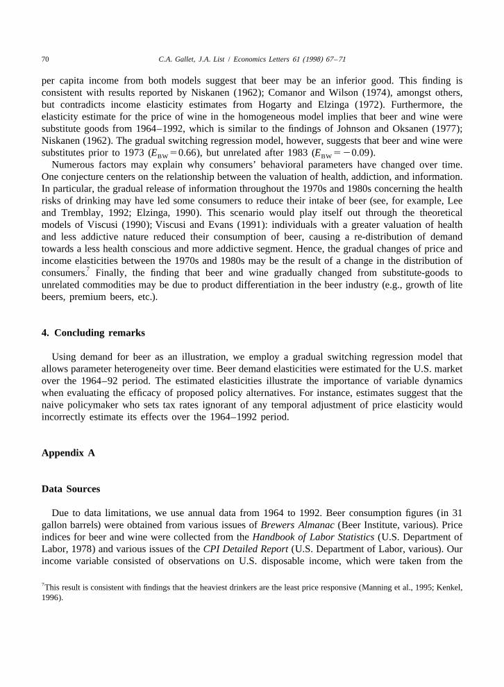
per capita income from both models suggest that beer may be an inferior good. This finding isconsistent with results reported by Niskanen (1962); Comanor and Wilson (1974), amongst others,but contradicts income elasticity estimates from Hogarty and Elzinga (1972). Furthermore, theelasticity estimate for the price of wine in the homogeneous model implies that beer and wine weresubstitute goods from 1964–1992, which is similar to the findings of Johnson and Oksanen (1977);Niskanen (1962). The gradual switching regression model, however, suggests that beer and wine weresubstitutes prior to 1973 (E 50.66), but unrelated after 1983 (E 520.09).BW BW
Numerous factors may explain why consumers’ behavioral parameters have changed over time.One conjecture centers on the relationship between the valuation of health, addiction, and information.In particular, the gradual release of information throughout the 1970s and 1980s concerning the healthrisks of drinking may have led some consumers to reduce their intake of beer (see, for example, Leeand Tremblay, 1992; Elzinga, 1990). This scenario would play itself out through the theoreticalmodels of Viscusi (1990); Viscusi and Evans (1991): individuals with a greater valuation of healthand less addictive nature reduced their consumption of beer, causing a re-distribution of demandtowards a less health conscious and more addictive segment. Hence, the gradual changes of price andincome elasticities between the 1970s and 1980s may be the result of a change in the distribution of
7consumers. Finally, the finding that beer and wine gradually changed from substitute-goods tounrelated commodities may be due to product differentiation in the beer industry (e.g., growth of litebeers, premium beers, etc.).
4. Concluding remarks
Using demand for beer as an illustration, we employ a gradual switching regression model thatallows parameter heterogeneity over time. Beer demand elasticities were estimated for the U.S. marketover the 1964–92 period. The estimated elasticities illustrate the importance of variable dynamicswhen evaluating the efficacy of proposed policy alternatives. For instance, estimates suggest that thenaive policymaker who sets tax rates ignorant of any temporal adjustment of price elasticity wouldincorrectly estimate its effects over the 1964–1992 period.
Appendix A
Data Sources
Due to data limitations, we use annual data from 1964 to 1992. Beer consumption figures (in 31gallon barrels) were obtained from various issues of Brewers Almanac (Beer Institute, various). Priceindices for beer and wine were collected from the Handbook of Labor Statistics (U.S. Department ofLabor, 1978) and various issues of the CPI Detailed Report (U.S. Department of Labor, various). Ourincome variable consisted of observations on U.S. disposable income, which were taken from the
7This result is consistent with findings that the heaviest drinkers are the least price responsive (Manning et al., 1995; Kenkel,1996).
C.A. Gallet, J.A. List / Economics Letters 61 (1998) 67 –71 71
Economic Report of the President (Council of Economic Advisors, 1995). To convert consumptionand income into per capita terms, we divided beer consumption and disposable income by the U.S.population (of persons 18 and over), which was obtained from various issues of Current PopulationReports (U.S. Department of Commerce, various). In addition to the price of wine, per capita income,and a linear time trend, instruments used to estimate beer demand consisted of the hourly beerproduction wage, beer industry material cost, the average state excise tax per barrel, and the numberof breweries operating, all of which was collected from various issues of Brewers Almanac. Finally,beer and wine prices, as well as per capita income, were deflated by the consumer price index; whilethe hourly beer production wage, beer industry material cost, and average state excise tax per barrelwere deflated by the producer price index. Data on both deflators were taken from the EconomicReport of the President.
References
Beer Institute. Brewers Almanac, (various issues), Washington, D.C.Baltagi, B., Levin, D., 1986. Estimating dynamic demand for cigarettes using panel data: The effects of bootlegging,
taxation, and advertising reconsidered. Review of Economics and Statistics 68, 148–155.Bishop, J., Yoo, J., 1985. Health scare, excise taxes, and the advertising ban in the cigarette demand and supply. Southern
Economic Journal 51, 402–410.Comanor, W., Wilson, T., 1974. Advertising and Market Power. Harvard University Press, Cambridge MA.Council of Economic Advisors, 1995. Economic Report of the President. Washington, D.C.Elzinga, K., 1990. The beer industry. In: Adams, W. (Ed.), The Structure of American Industry. Macmillan, New York NY.Hamilton, J., 1974. The demand for cigarettes: Advertising, the health scare, and the cigarette advertising ban. Review of
Economics and Statistics 54, 401–411.Hogarty, T., Elzinga, K., 1972. The demand for beer. Review of Economics and Statistics 54, 195–198.Horowitz, I., Horowitz, A., 1965. Firms in a declining market: The brewing case. Journal of Industrial Economics 13,
129–153.Johnson, J., Oksanen, E., 1977. Estimation of demand for alcoholic beverages in Canada from pooled time series and cross
sections. Review of Economics and Statistics 59, 113–118.Kenkel, D., 1996. New estimates of the optimal tax on alcohol. Economic Inquiry 34, 296–319.Lee, B., Tremblay, V., 1992. Advertising and the U.S. market demand for beer. Applied Economics 24, 69–76.Manning, W., Blumberg, L., Moulton, L., 1995. The demand for alcohol: The differential response to price. Journal of Health
Economics 14, 123–148.Niskanen, W., 1962. The Demand for Alcoholic Beverages. Unpublished Ph.D. Dissertation, University of Chicago.Ohtani, K., Katayama, S., 1985. An alternative gradual switching regression model and its application. Economic Studies
Quarterly 36, 148–153.Ohtani, K., Kakimoto, S., Abe, K., 1990. A gradual switching regression model with a flexible transition path. Economics
Letters 32, 43–48.Pollack, R., Wales, T., 1969. Estimation of the linear expenditure system. Econometrica 37, 611–628.U.S. Department of Commerce, Bureau of the Census. Current Population Reports, (various issues), Washington, D.C.U.S. Department of Labor, 1978. Handbook of Labor Statistics. Washington, D.C.U.S. Department of Labor. CPI Detailed Report, (various issues), Washington, D.C.Viscusi, W., 1990. Do smokers underestimate risks?. Journal of Political Economy 98, 1253–1269.Viscusi, W., Evans, W., 1991. Utility functions that depend on health status: Estimates and economic implications. American
Economic Review 80, 353–374.