BEC of Microcavity Polaritons - phyast.pitt.edusnoke/research/FinalThesis/FinalDissertation.pdf ·...

BOSE-EINSTEIN CONDENSATION OF

MICROCAVITY POLARITONS

by

Ryan Barrido Balili

B.S. Physics, MSU-Iligan Institute of Technology, 2002

M.S. Physics, University of Pittsburgh, 2005

Submitted to the Graduate Faculty of

the Department of Physics and Astronomy in partial fulfillment

of the requirements for the degree of

Doctor of Philosophy

University of Pittsburgh

2009

UNIVERSITY OF PITTSBURGH

DEPARTMENT OF PHYSICS AND ASTRONOMY

This dissertation was presented

by

Ryan Barrido Balili

It was defended on

June 11, 2009

and approved by

David W. Snoke, Professor, Physics and Astronomy

Hrvoje Petek, Professor, Physics and Astronomy

W. Vincent Liu, Assistant Professor, Physics and Astronomy

Robert Coalson, Professor, Chemistry

P. Kevin Chen, Assistant Professor, Electrical and Computer Engineering

Dissertation Director: David W. Snoke, Professor, Physics and Astronomy

ii

BOSE-EINSTEIN CONDENSATION OF MICROCAVITY POLARITONS

Ryan Barrido Balili, PhD

University of Pittsburgh, 2009

The strong coupling of light and excitons in a two-dimensional semiconductor microcavity

results in a new eigenstate of quasiparticles called polaritons. Microcavity polaritons have

generated much interest due to the wealth of interesting optical phenomena recently observed

in these systems such as nonlinear emission, macroscopic coherence, and bosonic stimulated

scattering. The efficiency of amplification, parametric oscillation, and coherent emission of

light makes it promising for applications in coherent control, microscopic optical switching,

and other opto-electronic devices. Most of all, because of their light mass and bosonic

character, these particles are predicted to undergo Bose-Einstein condensation (BEC) at

much higher temperatures and lower densities than their atomic counterparts.

Standard methods of growing semiconductor microcavities are quite inefficient in produc-

ing well-tuned samples with strong coupling of light and excitons. Wafers with continuously

varying thicknesses are often produced, leaving only tiny regions with strong coupling. In

our experiments, an inhomogeneous stress is applied to the microcavity in order to actively

couple naturally detuned exciton and cavity modes at fixed k|| = 0, and at the same time,

create an in-plane spatial trap, potentially making BEC of polaritons possible.

Our recent experiments with exciton-polaritons in the stress trap have shown compelling

evidence of BEC. At the bottom of the trap where the coupling is strongest, line narrowing

and nonlinear increase of photoluminescence intensity are observed. Also a single, spatially

narrow condensate of polariton gas is formed analogous to the case of atoms in a three-

dimensional harmonic potential. Above a critical density, we observe a massive occupation of

polaritons in the ground state, spontaneous build-up of linear polarization, and macroscopic

iii

coherence of the condensate all in agreement with predictions. The results are similar to what

is observed in the naturally resonant unstressed case. Comparison with the stressed trap

and the nonstressed case, however, revealed that stress traps play a significant contribution

in forming a polariton condensate. Furthermore, the stress trap case has shown, where the

unstressed case has not, two distinct thresholds, one from photon lasing and another from a

BEC transition.

Keywords: stress, trapped, polariton BEC, condensation, polaritons, semiconductor, mi-

crocavities.

iv

TABLE OF CONTENTS

PREFACE . . . . . . . . . . . . . . . . . . . . . . . . . . . . . . . . . . . . . . . . . xii

1.0 INTRODUCTION . . . . . . . . . . . . . . . . . . . . . . . . . . . . . . . . 1

1.1 Overview . . . . . . . . . . . . . . . . . . . . . . . . . . . . . . . . . . . . 1

1.2 Brief Survey of Microcavity Polariton Research . . . . . . . . . . . . . . . 3

1.3 Thesis Outline . . . . . . . . . . . . . . . . . . . . . . . . . . . . . . . . . 5

2.0 MICROCAVITY POLARITONS . . . . . . . . . . . . . . . . . . . . . . . 7

2.1 Coupled Quantum Oscillator Model . . . . . . . . . . . . . . . . . . . . . 7

2.2 Features of the Microcavity Polariton . . . . . . . . . . . . . . . . . . . . 10

2.2.1 Weakly Interacting and Light Mass . . . . . . . . . . . . . . . . . 10

2.2.2 Lifetime Variation in Momentum Space . . . . . . . . . . . . . . . 11

2.2.3 Bottleneck Effect . . . . . . . . . . . . . . . . . . . . . . . . . . . 12

2.2.4 Magic Angle . . . . . . . . . . . . . . . . . . . . . . . . . . . . . . 13

2.2.5 Polariton Spin and Polarization . . . . . . . . . . . . . . . . . . . 15

2.3 Transfer Matrix Formalism . . . . . . . . . . . . . . . . . . . . . . . . . . 16

2.4 Sample Design and Characteristics . . . . . . . . . . . . . . . . . . . . . . 19

3.0 MACROSCOPIC QUANTUM PHENOMENA IN POLARITON SYS-

TEMS . . . . . . . . . . . . . . . . . . . . . . . . . . . . . . . . . . . . . . . . 23

3.1 BEC in Microcavity Polaritons . . . . . . . . . . . . . . . . . . . . . . . . 23

3.2 Polariton Superfluidity . . . . . . . . . . . . . . . . . . . . . . . . . . . . 26

3.3 Stability of the Condensate . . . . . . . . . . . . . . . . . . . . . . . . . . 28

3.4 Phase-Space Filling and Transition to Weak Coupling . . . . . . . . . . . 30

3.5 Polariton Laser . . . . . . . . . . . . . . . . . . . . . . . . . . . . . . . . 31

v

3.6 Signatures of BEC . . . . . . . . . . . . . . . . . . . . . . . . . . . . . . . 34

4.0 TRAPPING POLARITONS . . . . . . . . . . . . . . . . . . . . . . . . . . 36

4.1 Tuning to Resonance and Trapping . . . . . . . . . . . . . . . . . . . . . 36

4.2 Characteristics of a Microcavity with a Stress Trap . . . . . . . . . . . . 39

4.2.1 Photoluminescence and Reflectivity . . . . . . . . . . . . . . . . . 39

4.2.2 Drift . . . . . . . . . . . . . . . . . . . . . . . . . . . . . . . . . . 41

4.2.3 Evaporative Cooling Effect . . . . . . . . . . . . . . . . . . . . . . 43

5.0 OPTICAL METHODS . . . . . . . . . . . . . . . . . . . . . . . . . . . . . 45

5.1 Imaging and Spectroscopic Techniques . . . . . . . . . . . . . . . . . . . 45

5.2 Measuring Coherence with a Michelson Interferometer . . . . . . . . . . . 47

6.0 EXPERIMENTAL RESULTS WITH CW LASER PUMPING . . . . 49

6.1 Stress and Polarization Power Series . . . . . . . . . . . . . . . . . . . . . 49

6.2 Angle-Resolved Measurements . . . . . . . . . . . . . . . . . . . . . . . . 53

6.2.1 Angle-Resolved Power Series . . . . . . . . . . . . . . . . . . . . . 53

6.2.2 Occupation at Different Detuning and Stress . . . . . . . . . . . . 54

6.3 Real-Space Distribution . . . . . . . . . . . . . . . . . . . . . . . . . . . . 57

6.4 Measurement of Spatial Coherence . . . . . . . . . . . . . . . . . . . . . . 58

6.5 Comparison of Trapped and Untrapped Case . . . . . . . . . . . . . . . . 60

7.0 EXPERIMENTAL RESULTS WITH MODULATED QUASI-CW PUMP-

ING . . . . . . . . . . . . . . . . . . . . . . . . . . . . . . . . . . . . . . . . . 67

7.1 Diffusion and Trapping at the Center of the well . . . . . . . . . . . . . . 67

7.2 Side Pumping Power Series . . . . . . . . . . . . . . . . . . . . . . . . . . 68

7.3 Side-Pumping Real Space Distribution . . . . . . . . . . . . . . . . . . . 71

7.4 Angle-Resolved Measurements . . . . . . . . . . . . . . . . . . . . . . . . 71

7.5 Polarization Measurements . . . . . . . . . . . . . . . . . . . . . . . . . . 74

8.0 EXPERIMENTAL MEASUREMENTS OF STRESS INDUCED SPLIT-

TING . . . . . . . . . . . . . . . . . . . . . . . . . . . . . . . . . . . . . . . . 76

9.0 CONCLUSION . . . . . . . . . . . . . . . . . . . . . . . . . . . . . . . . . . 82

10.0 FUTURE DIRECTIONS . . . . . . . . . . . . . . . . . . . . . . . . . . . . 84

APPENDIX A. DEFINITION OF POLARITON HAMILTONIAN MATRIX 86

vi

APPENDIX B. QUANTUM THEORY OF EXCITON-POLARITONS . . 88

APPENDIX C. MICROCAVITY STRUCTURE . . . . . . . . . . . . . . . . . 98

APPENDIX D. DENSITY OF STATES FOR A D-DIMENSIONAL POWER

LAW TRAP . . . . . . . . . . . . . . . . . . . . . . . . . . . . . . . . . . . . 99

APPENDIX E. PIKUS-BIR HAMILTONIAN AND EXCHANGE TERM 102

APPENDIX F. TRANSFER MATRIX SIMULATION CODE . . . . . . . . 106

APPENDIX G. MATLAB CODE FOR STRESS ANALYSIS . . . . . . . . . 119

G.1 Function for Pikus-Bir and Exchange Calculation . . . . . . . . . . . . . 119

G.2 Main Executable File . . . . . . . . . . . . . . . . . . . . . . . . . . . . . 128

APPENDIX H. ANSYS INPUT FILE . . . . . . . . . . . . . . . . . . . . . . . 135

BIBLIOGRAPHY . . . . . . . . . . . . . . . . . . . . . . . . . . . . . . . . . . . . 143

vii

LIST OF TABLES

2.1 Parameters used for simulations shown in Fig. 2.6 . . . . . . . . . . . . . . . 21

8.1 Relevant parameters used for simulations shown in Fig. 8.3 . . . . . . . . . . 80

viii

LIST OF FIGURES

1.1 Criteria for achieving BEC . . . . . . . . . . . . . . . . . . . . . . . . . . . . 2

2.1 Structure of microcavities, exciton-photon coupling and dispersion relation . 10

2.2 Scattering rate of polaritons via longtitudinal optical phonon emission . . . . 13

2.3 Optical parametric oscillation . . . . . . . . . . . . . . . . . . . . . . . . . . 14

2.4 Polarization of the optical transitions in GaAs quantum wells . . . . . . . . . 15

2.5 Normal incidence reflectivity and simulation . . . . . . . . . . . . . . . . . . 18

2.6 Anti-crossing of the upper and lower polariton . . . . . . . . . . . . . . . . . 20

2.7 Reflectivity spectrum as a function of position . . . . . . . . . . . . . . . . . 22

4.1 Geometry of the stress technique and the structure of the microcavity . . . . 37

4.2 Different possible tunings with increasing stress . . . . . . . . . . . . . . . . 38

4.3 Profile of the stress well . . . . . . . . . . . . . . . . . . . . . . . . . . . . . . 39

4.4 Photoluminescence and reflectivity of a stress trap . . . . . . . . . . . . . . . 40

4.5 Photoluminescence and reflectivity spectra vs. stress . . . . . . . . . . . . . . 41

4.6 Polariton drift and trapping . . . . . . . . . . . . . . . . . . . . . . . . . . . 42

4.7 Photon fraction of the lower polariton across the trap . . . . . . . . . . . . . 43

5.1 Experimental setup for spectral and spatial imaging . . . . . . . . . . . . . . 45

5.2 Experimental setup for angle-resolved measurements with a diffuser plate . . 46

5.3 Michelson interferometer setup for first order coherence measurements . . . . 47

6.1 Photoluminescence intensity at k‖ = 0 versus pump power . . . . . . . . . . . 50

6.2 Total intensity, full width at half maximum, and polarization . . . . . . . . . 51

6.3 Polarization below and above threshold for different sample orientations . . . 52

6.4 Angle resolved measurements . . . . . . . . . . . . . . . . . . . . . . . . . . . 53

ix

6.5 Occupation number from angle resolved measurements . . . . . . . . . . . . . 54

6.6 Comparison of the occupation at different detunings . . . . . . . . . . . . . . 55

6.7 Occupation at different trap frequencies . . . . . . . . . . . . . . . . . . . . . 56

6.8 Series of spectral profiles at different pump powers . . . . . . . . . . . . . . . 56

6.9 Two dimensional spatial profiles for a series of powers . . . . . . . . . . . . . 58

6.10 Spatial coherence using Michelson interferometer . . . . . . . . . . . . . . . . 59

6.11 Untrapped case photon lasing thresholds . . . . . . . . . . . . . . . . . . . . 61

6.12 Untrapped case photon lasing transition . . . . . . . . . . . . . . . . . . . . . 62

6.13 Trapped case photon lasing and BEC thresholds . . . . . . . . . . . . . . . . 65

6.14 Trapped case photon lasing and BEC transition . . . . . . . . . . . . . . . . 66

7.1 Diffusion and trapping at the center of the well . . . . . . . . . . . . . . . . . 68

7.2 Side pumping power series . . . . . . . . . . . . . . . . . . . . . . . . . . . . 69

7.3 Side pumping intensity, FWHM, and polariton branches . . . . . . . . . . . . 70

7.4 Two-dimensional spatial profile of the emission at k|| = 0± 5.2 . . . . . . . . 72

7.5 Quasi-CW Angle-resolved light emission . . . . . . . . . . . . . . . . . . . . . 73

7.6 Quasi-CW number of polaritons per k-state . . . . . . . . . . . . . . . . . . . 74

7.7 Total intensity, FWHM, and polarization of Quasi-CW pump . . . . . . . . . 75

8.1 Example of polariton splitting . . . . . . . . . . . . . . . . . . . . . . . . . . 76

8.2 Actual LP splitting and series of splitting with stress . . . . . . . . . . . . . 77

8.3 Pikus-Bir and exchange LP splitting simulations . . . . . . . . . . . . . . . . 79

C1 Layer structure of the semiconductor microcavity sample . . . . . . . . . . . 98

E1 Stress well fit example from DQW experiments . . . . . . . . . . . . . . . . . 104

x

To my greatest mentors, my parents, George and Mercy, who taught me how to live and,

more importantly, how to love.

xi

PREFACE

Before anything I else, I thank God for the strength he has given me all these years to

continue my studies here in University of Pittsburgh. To Him belongs all glory and honor!

This thesis would not have been possible if not for my wife, Nikki, who has been my

constant support and ecouragement all these years. Your encouragement has made our

challenges more bearable. Life has been so much more enjoyable since you came along.

I am thankful for the encouragement of my parents, my brother and my sisters.

The results of my experiments and my progress as a student would not have reached

its completion with out the support and guidance of my supervisor Prof. David Snoke. He

never left me behind and was with me from beginning to the end. To him I express my

gratitude.

I am thankful for my committee members, K. Chen, H. Petek, V. Liu, and R. Coalson

for taking time to watch my progress as a graduate student.

I am also grateful for Yingmei Liu and Sava Denev who showed me the ways of the lab

when I was still new with the group.

I would like to thank V. Hartwell, Z. Voros, B. Zhang, C. Yang, B. Nelsen, J. Wuenschell,

N. Sinclair, and A. Heberle for their invaluable comments, discussions, and help in many of

my experiments. I would like to give special mention to B. Giles, K. Petrocelly and K. Kotek

whom I had the pleasure working with in the machine shop. I thank them for the friendship

and the wonderful times we spent working, learning, and playing together when we had the

chance.

I am also indebted to Engr. R.H. Reid for helping me with the stress simulations using

ANSYS. It would have taken me a long time to finish the final part of my PhD work with

out his assistance.

xii

Furthermore, this dissertation would not be possible if not for the semiconductor micro-

cavity samples sent by L. Pfeiffer and K. West from Bell Labs. I am also grateful to our

collaborators in Stanford University and H. Deng, G. Weihs, and Y. Yamamoto for contri-

butions to the initial design of the samples. The preliminary research has been supported

by the National Science Foundation under Grant No. 0404912 and by DARPA under Army

Research Office Contract No. W911NF-04-1-0075.

Ryan B. Balili

Pittsburgh, PA

xiii

1.0 INTRODUCTION

1.1 OVERVIEW

In 1925, after generalizing Satyendra Nath Bose’s work on the statistics of monoatomic

ideal gases, Albert Einstein speculated that, at very low temperatures, a certain type of

identical particles, now called bosons, would “collapse” or condense into its lowest energy

state. This particle state is called the Bose-Einstein condensate (BEC). Previously observed

macroscopic quantum phenomena like superfluidity and superconductivity were later suc-

cessfully explained by the theory of BEC [1, 2, 3, 4]. In 1995, two independent teams,

from NIST-JILA and MIT, lead by Eric Cornell and Wolfgang Ketterle, respectively, ver-

ified the Bose-Einstein condensation of rubidium and sodium atoms experimentally [5, 6],

earning them the Nobel Prize for Physics in 2001. How did this interesting phenomenon

come about? The explanation lies at the very heart of quantum theory. According to

Louis de Broglie’s postulate on wave-particle duality, all matter and radiation have wave

and particle aspects. The associated wavelength of a particle is given by Planck’s constant

h = 6.63×10−34 kg·m2/s divided by the particle’s momentum p i.e λ = h/p. A particle’s aver-

age velocity corresponds to the temperature in thermal equilibrium, given by v =√

3kBT/m

where kB = 1.38× 10−23 kg ·m2/(K · s2) is Boltzmann’s constant. In other words, p ∝√mT

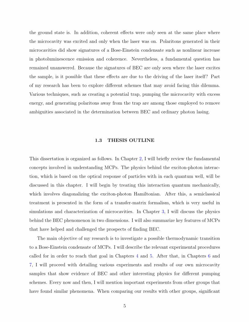
or λ ∝ 1/√mT . At very low temperatures or with extremely light particles, the particle’s

momentum becomes so small that the de Broglie wavelength becomes comparable to the

distance between particles (see Figure 1.1). The particles, or wave-packets in the wave na-

ture point of view, start “adding up” or superposing constructively. A highly ordered state

arises such that a macroscopic collection of these particles becomes dependent on a single

wave function. All the particles thus behave in the same manner, spectacularly amplifying

1

the quantum nature of the individual particles.

Figure 1.1: Criteria for achieving BEC. Left: Forheavier particles temperatures must be decreaseda lot to increase de Broglie wavelength. Right:For lighter particles, associated wavelength’s arelonger. Decreasing the distance between particlesby increasing density can be an open variable forcreating a condensate. In both methods, the samemacroscopic condensate or wave comes out in theend.

The critical temperature for BEC of atoms is remarkably low. Atomic BEC physicists

often boast of their system as the coldest place in the universe, down to the nanokelvin

temperatures. Reaching close to absolute zero temperature was such a daunting feat in

itself. It required advanced cryogenic systems and sophisticated techniques some of which

have earned their own Nobel Prize (e.g. method of laser cooling [7]). Though BEC opened

doors to new physics, it is imperative that we increase its critical temperature for any

practical applications. This can be achieved if we use particles with far smaller mass (see

Fig. 1.1). This is where polaritons come in.

Microcavity polaritons (MCPs) have in the past decade been the object of great interest

for many scientists [8, 9, 10, 11, 12, 13, 14, 15, 16, 17, 18, 19] for its phenomenal optical

properties and for those interested in the study of BEC. A polariton is a mixed state of a

bound electron-hole pair and a photon. Electron-hole pairs are created when an electron is

excited in a semiconductor and leaves a hole in the lattice. Given the right conditions, the

electron binds with a positively charged hole, forming an exciton, a quasi-particle very much

like a hydrogen atom. When an exciton couples with a photon, a polariton is created which

2

is a superposition of its original components. Polaritons are very light particles, making

BEC possible even at room temperature.

Polaritons decay by emitting light with energy and momentum corresponding to the

state of the polariton. The lifetime is short in semiconductor microcavities, as it is mainly

dependent on how long the photon stays in the cavity. A microcavity is made up of two

highly reflective mirrors facing each other. Sandwiched in the microcavity are quantum wells

where the excitons are created. When trapped in an optical cavity, the photons couple with

the excitons much more effectively, creating a strongly coupled polariton state. Increasing

the quality of the mirrors increases the lifetime of the polaritons. Given sufficient density

of particles, some will be able to scatter to the lowest energy state. Once a polariton

occupies the lowest energy state, scattering to that state is enhanced considerably, leading

to a macroscopic condensate. As the polariton condensate decays, intense coherent and

monochromatic light is emitted. This spontaneous coherence effect has inspired the creation

of new opto-electronic devices, namely the “polariton laser”. Below a critical temperature,

this new generation of “lasers” would not require population inversion and would have very

low thresholds.

1.2 BRIEF SURVEY OF MICROCAVITY POLARITON RESEARCH

The study of exciton-polaritons in bulk materials began as early as 1958 with J. Hopfield[20]

who first suggested the linear coupling of electronic excitations to the electromagnetic field.

Application of the polariton concept to lower dimensional systems was later investigated in

quantum wells (QWs) but failed to show evidence of normal-mode coupling since a two-

dimensional (2D) QW exciton couples to a three-dimensional (3D) continuum of photon

modes leading to an enhanced radiative decay[21, 22]. The first successful observation of

strong coupling in two dimensions was made in 1992 by C. Weisbuch[23] in a semiconductor

microcavity. By then, technological advancement in growing heterostructures allowed the

manufacture of highly reflective dielectric mirrors. Photons, even those that are normal

to the cavity, i.e. with zero in-plane momenta, lived long enough for the vacuum-field

3

Rabi oscillation frequency, which is proportional to the coupling strength, to be faster than

the escape rate[24]. At that time, observations were understood as a semiclassical linear

coupling of excitons to an light field in analogy with atoms in a resonant optical cavity[25].

Soon after, an equivalent quantum description was developed[26, 27], treating a quantized

excitation coupled with a quantized light field.

The BEC transition in MCPs was first suggested by Imamoglu et. al.[28] in 1996. Not

long after, evidence of final-state stimulation in microcavity systems under non-resonant

excitation was reported[29, 30, 31, 8, 9]. Non-resonant pumping means generating carriers

that have different energy from the final state of interest. This can be done by exciting either

with high energy or with large in-plane momentum so that carriers emit many phonons,

thereby losing coherence, before reaching the final state. Populating the ground state can

also be done more directly using resonant excitation. This is achieved by simply pumping

the low polariton energy levels with energy close to the ground state. Population build

up of polaritons is more efficient using resonant excitation than using high-energy non-

resonant excitation, where carriers are subject to decay during thermalization and suppressed

relaxation caused by the “bottleneck effect”(see Section 2.2). However, in resonant pumping,

residual coherence from the laser may affect the correlation observed in the ground state[32].

Resonant pumping also can give rise to parametric scattering process (see Section 2.2). These

effects are interesting in themselves, with a variety of important applications, from coherent

control[12] to creating entangled polariton states[33]. Nevertheless, the correlated behavior

observed cannot be described in the physics of spontaneous thermodynamic phase transition,

although this has been debated recently[34].

Our interest, however, is nonresonant excitation, i.e., incoherent pumping of particles.

Several nonresonant excitation schemes have already indicated spontaneous coherence of

polariton gas in various two-dimensional microcavity structures at around 4 Kelvin (e.g.

Refs. [14, 8]). Though this is still not room temperature, it is a big improvement on the

nanokelvin temperatures in atomic BEC. However, in these experiments, no confining poten-

tial was applied to trap the polaritons. In their systems, polaritons are generated only where

the laser is focused. Polaritons diffuse freely away from the excitation region and fall into the

local minima created either by disorder or the laser itself. This makes it hard to define what

4

the ground state is. In addition, coherent effects were only seen at the same place where

the microcavity was excited and only when the laser was on. Polaritons generated in their

microcavities did show signatures of a Bose-Einstein condensate such as nonlinear increase

in photoluminescence emission and coherence. Nevertheless, a fundamental question has

remained unanswered. Because the signatures of BEC are only seen where the laser excites

the sample, is it possible that these effects are due to the driving of the laser itself? Part

of my research has been to explore different schemes that may avoid facing this dilemma.

Various techniques, such as creating a potential trap, pumping the microcavity with excess

energy, and generating polaritons away from the trap are among those employed to remove

ambiguities associated in the determination between BEC and ordinary photon lasing.

1.3 THESIS OUTLINE

This dissertation is organized as follows. In Chapter 2, I will briefly review the fundamental

concepts involved in understanding MCPs. The physics behind the exciton-photon interac-

tion, which is based on the optical response of particles with in each quantum well, will be

discussed in this chapter. I will begin by treating this interaction quantum mechanically,

which involves diagonalizing the exciton-photon Hamiltonian. After this, a semiclassical

treatment is presented in the form of a transfer-matrix formalism, which is very useful in

simulations and characterization of microcavities. In Chapter 3, I will discuss the physics

behind the BEC phenomenon in two dimensions. I will also summarize key features of MCPs

that have helped and challenged the prospects of finding BEC.

The main objective of my research is to investigate a possible thermodynamic transition

to a Bose-Einstein condensate of MCPs. I will describe the relevant experimental procedures

called for in order to reach that goal in Chapters 4 and 5. After that, in Chapters 6 and

7, I will proceed with detailing various experiments and results of our own microcavity

samples that show evidence of BEC and other interesting physics for different pumping

schemes. Every now and then, I will mention important experiments from other groups that

have found similar phenomena. When comparing our results with other groups, significant

5

differences will be pointed out. In Chapter 8, I will present the latest feature observed and

measured in stressed microcavities, namely the splitting of the polaritons states with stress.

The current accepted theory for the splitting will be presented. I will also include simulations

and numerical fits to the splitting data. Finally, I will give my conclusions in Chapter 9.

Details of important calculations, simulations, and theories are attached in the Appendix.

6

2.0 MICROCAVITY POLARITONS

2.1 COUPLED QUANTUM OSCILLATOR MODEL

A semiconductor microcavity is made up of a Fabry-Perot cavity sandwiched between two

reflectors facing each other with quantum wells (QWs) embedded in between. The reflectors,

called distributed Bragg reflectors (DBRs), are made up of alternating quarter-wave layers of

semiconductor materials with high and low indices of refraction. Confinement in the cavity

leads to the quantization of the photon energy in the growth direction while the in-plane

photon states remain unaffected. The exciton states of the embedded quantum wells also

exhibit similar quantization in the growth direction and continuous states in the free in-plane

motion. If the exciton and the cavity modes are in resonance with each other, the coupling of

light and excitons occurs, creating the mixed matter-light quasi-particles we call polaritons.

The dispersion relations of bare exciton and light mode no longer exist in this regime but

two distinct dispersion called the polariton branches.

The bare cavity photon dispersion relation can be easily derived noting that the DBR’s

force the axial wave vector kz to be quantized (see illustration on Fig. 2.1). Hence

Eph = hck = hc√k2z + k2

|| = hc

[(Nπ

neffLc

)2

+ k2||

]1/2

(2.1)

where kz is along the epitaxial growth direction, k|| is the wavevector parallel to the quantum

well, Lc is the effective cavity length, neff is the effective intracavity index of refraction, and

N is the mode number or the number of half-wavelengths in the cavity. For our microcavity

(neff ≈ 3.6, L ≈ 320 nm), the mode spacing is 0.54 eV. Our microcavity (see structure in

Appendix C) was designed to for an N = 3 cavity mode resonance, which means there are

7

three antinodes in the cavity. Quantum wells are placed in the antinodes, where the field

intensity is maximum. This ensures optimum overlap between the exciton and the photon

field.

The exciton in a QW has energy

Eex = E0 +h2k2

||

2(me +mh)(2.2)

where E0 is the ground state exciton energy and me(mh) is the electron(hole) in-plane mass.

Notice that the photon and the exciton is given the same in-plane momentum k||. This is due

to momentum conservation required by the in-plane translational invariance of the system.

This results in the coupling of an exciton and photon with the same in-plane wave vector.

We can then treat the exciton and photon modes as coupled oscillators with coupling

matrix element Ω. Using the exciton state |ex〉 and photon state |ph〉 as basis, the coupling

is described by the matrix Hamiltonian (see Appendix A):

H =

Eex Ω/2

Ω/2 Eph

(2.3)

where Eph and Eex are the energies of the cavity photon and exciton mode respectively. The

eigenvectors of this Hamiltonian is a superposition of the exciton and photon states which

can be represented as

|UP 〉 = C |ex〉+X |ph〉

|LP 〉 = X |ex〉 − C |ph〉 (2.4)

where

X2 =1

2+

Eph − Eex

2√

(Eph − Eex)2 + Ω2

and C2 = 1− X2 (2.5)

are the standard Hopfield coefficients[20, 35] describing the fraction of the exciton and the

photon content of the polariton. The two coupled mode eigenstates of the system are called

8

the upper polariton (UP) and the lower polariton (LP), corresponding to the higher and the

lower energy states, respectively. Diagonalizing the Hamiltonian we get the eigen energies

EUPLP

=Eex + Eph

2±

[(Eex − Eph

2

)2

+

(Ω

2

)2]1/2

. (2.6)

The energy splitting of these two modes at resonance is referred to as the Rabi splitting

(Ω/2) or the coupling constant (Ω). It is a function of the quantum oscillator strength

f which contains the electric dipole matrix elements of the atomic transitions. It is also

dependent on the number of atomic oscillators which is proportional to the number of QWs.

To trace the physics behind the coupling term Ω and oscillator strength f , a more detailed

derivation from the quantum theory of a classical dielectric is presented in Appendix B. The

coupling constant can be determined experimentally by measuring the minimum splitting

between the UP and LP spectral lines1. If we include exciton broadening δex and cavity line

broadening δph, a more realistic form the UP and LP energies is given by

EUPLP

=Eex + Eph − i (δex + δph)

2±

[(Eex − Eph − i (δex − δph)

2

)2

+

(Ω

2

)2]1/2

. (2.7)

When the splitting is larger than the difference in line widths of the exciton and the cavity

lines (|δex − δph| Ω), then the system is considered to be in the strong-coupling regime.

Because of the finite lifetime of the photon component, MCPs convert directly into

external photons. The direct correspondence of the polariton state inside the cavity with

the outgoing photons allows one to easily examine its dispersion curve in reflectivity and

luminescence measurements. Note that sin θ = k||/k. Using the equation of the cavity

photon dispersion we get the relationship between the k|| wave vector and the angle (θ) as

k|| =Eph

hcsin θ. Hence, a particular k||-mode can be accessed simply by selecting the angle (θ)

of the pump laser injection. In the same way, by recording the PL spectra as a function of

emission angle, we can get a complete measurement of the momentum and energy distribution

of polaritons.

1Typical values of the Rabi splitting are in the order of meV. It is also worth pointing out that the typicalvalues of the longitudinal-transverse (LT) splitting are of the order of µeV [35] and are only significant atincident or emission angles far from normal.

9

k||

E

Eph

Eex

UP

LP

Figure 2.1: Left: Basic structure of microcavities and illustration of the photon-exciton oscillatorcoupling. Right: Dispersion relation of the upper and lower polariton (solid curves).

In our experiments, a reservoir of free carriers are first created in the electron-hole con-

tinuum by pumping the microcavity with a high energy laser 130 meV above LP energy. The

carriers cool subsequently by emitting phonons. As the carriers lose energy, they bind into

excitons and interact with cavity photons populating the polaritons states. This pumping

scheme allows the particles to lose coherence imparted by the pump laser. Polaritons decay

by emitting photons corresonding to its state in the dispersion which can then be measured

using standard techniques of photoluminescence spectroscopy.

2.2 FEATURES OF THE MICROCAVITY POLARITON

2.2.1 Weakly Interacting and Light Mass

It is well established [36] that MCPs behave as a gas of weakly interacting bosons. The

cavity photons are essentially non-interacting. Polaritons owe their short-range interaction

to their exciton components. The the half-light, half-exciton character of the polaritons,

with the photon component having a very steep dispersion, gives it a very small in-plane

10

mass. For the sample used in our experiments, we measured the mass2 of the polaritons

to be 7 × 10−5 times the vacuum electron mass [37]. This makes MCPs very interesting to

study in relation to BEC and in relation to a new generation of opto-electronic devices that

can be designed based on the BEC of polaritons. In addition, the distinct dispersion of this

system has produced a wealth of interesting optical phenomena such as nonlinear emission,

polaritonic amplification, and reports of bosonic stimulated scattering [8, 9, 10, 15].

2.2.2 Lifetime Variation in Momentum Space

The lifetime of excitons in the QWs is in the order of nanoseconds. Polaritons, however,

are a mix of excitons and photons, making their lifetime much shorter than the exciton

lifetime. In the microcavity, the polariton lifetime is very much limited by the quality of

the DBRs. The higher the reflector quality, or Q-factor, the longer the photon stays in the

cavity, the longer the polariton lifetime. The value of the Q-factor, Q = λc/∆λc, where λc is

the cavity resonance, is equivalent to the average number of round trips of a photon inside

the cavity. For our MC sample, with cavity resonance λc = 775.7 nm and resonance width

of ∆λc = 0.2 nm, Q ≈ 3880. The estimated photon lifetime, τph = 2neffLQ/c, in the cavity

is about 30 ps, where the effective cavity index neff ≈ 3.6, cavity length L ≈ 320 nm and c

is the speed of light.

Quantitatively, the polariton lifetime τ depends on the fraction and lifetime of each

individual photon and exciton component, according to

τ =

(fphτph

+fexτex

)−1

, (2.9)

where fph(fex) and τph(τex) are the photon(exciton) fraction and the bare photon(exciton)

lifetime. Note that fex = 1− fph where fex = X2 and fph = C2 from Eq. (2.5). The amount

2The effective mass m is given by

m =h2

d2E(k||)/dk2||, (2.8)

where E(k||) is the energy dispersion and k|| is the in-plane momentum. The curvature d2E(k||)/dk2|| can be

calculated by fitting the dispersion relation, deduced from angle-resolved measurements (e.g. Fig. 7.5), witha parabola.

11

of mixing is dependent on the particular shape of the photon and exciton dispersion E(k||).

The photon fraction fph is given by[35]

fph =1

2−

Eph(k||)− Eex(k||)

2√(

Eph(k||)− Eex(k||))2

+ Ω2

(2.10)

where Eph is the cavity photon energy and Eex is the exciton energy for a particular in-plane

wavevector k||, and Ω is the coupling constant. Hence, polaritons in the ground state have

a much shorter lifetime compared to polaritons at higher energy states. This is detrimental

to creating a condensate in thermal equilibrium. For the sample studied, at resonance,

the lifetime of the lower polaritons was measured, using second harmonic cross-correlation,

to be about 7.7 ps [38], which is comparable to polariton lifetime reported elsewhere in

similar structures [9]. Fortunately, absolute time scales are irrelevant in the BEC transition.

What matters is the thermalization time compared to the lifetime of the polaritons, and the

thermalization time can be in the sub-picosecond range.

Knowledge of the lifetime variation in momentum space is also important later in Chap-

ter 6.2 and Chapter 7.4 for converting from raw PL intensity to occupation number. For a

constant number of polaritons, the shorter the lifetime of a polariton, the more intense the

PL, since at a given detection time more particles decay from a particular state. The PL

intensity is converted to occupation number by the lifetime correction.

2.2.3 Bottleneck Effect

Another important feature of the polaritons is called the “bottleneck effect” which arises

due to the steep region of the the lower polariton branch and the reduced exciton fraction

in as the polaritons become more photonlike. Ideally, optically excited electrons and holes

that are created in the quantum well form excitons and thermalize through interaction

with each other, with other free carriers, and by interacting the lattice phonons. However,

thermalization due to scattering with phonons is much slower as polaritons become more

photonlike[39, 38]. In addition, as discussed in the previous section, recombination times

are much shorter for photonlike polaritons. These effects result in a depletion region near

the zone center and a reduced polariton relaxation in that area. In the “bottleneck” region,

12

phonons cannot provide an efficient polariton relaxation because of a reduced density of

states (see Fig. 2.2). Nevertheless, our group [40] and others [30, 41] have seen a nonlinear

increase in luminescence from the ground state even with non-resonant optical pumping.

These results suggest that other relaxation mechanisms overcome this “bottleneck”. The

primary mechanism is polariton-polariton scattering [38]. If has also been suggested that

free carrier scattering with polaritons may play a role [38, 11].

0 1 2 3 4 5 61.0

1.2

1.4

1.6

1.8

2.0

2.2

Pol

arito

n - L

O P

hono

n R

atre

k|| (104 cm-1)

0 1 2 3 4 5 6

k|| (104 cm-1)

Den

sity

of S

tate

s (A

rb. U

nits

)

Figure 2.2: Left: Scattering rate of polaritons via longtitudinal optical phonon emission solved usingFermi Golden Rule[42, 38]. Right: Density of states of the lower polariton.

2.2.4 Magic Angle

The shape of the lower polariton branch allows energy-momentum conserving scattering

processes into the polariton ground state at a particular in-plane wavenumber k often called

the “magic angle”(see Fig. 2.3). Two polaritons under resonant pumping can scatter into

zero and 2k states with energies E0 and E2k such that 2Ek = E0 + E2k. Basically, an

optical parametric oscillation is achieved where the signal (E0) and idler (E2k) pair created

leaves the microcavity at different angles corresponding to their k state [43, 44, 12, 45]. This

parametric processes has been shown to have long coherence times[12], making them ideal

for coherent-control applications. The short duration and efficiency of amplification also

13

Eex

Eph

LP

UP

k 2k0

E0

E2k

Ek

k||

E

signal

pump

idler

Figure 2.3: Dispersion curve showing optical para-metric scattering when pumping resonantly at themagic angle corresponding to 2k-wavevector.

makes it promising for applications in high-speed microscopic optical switching, and other

opto-electronic devices.

There are two experimental schemes involving parametric processes in microcavity po-

laritons that are being widely studied. The first is called parametric amplification[43], where

a resonant laser probes the signal. The probe beam effectively intitiates the parametric

process, which subsequently amplifies the signal intensity as the the pump is converted to

signal and idler. This behavior can be explained classically[46, 47] as a non-linear four-wave

mixing effect satisfying the energy conservation condition

2Fp(ωp, ~kp) = Fs(ωs, ~ks) + Fi(ωi, ~ki) , (2.11)

where Fp, Fs, and Fi correspond to pump, signal, and idler field amplitudes with their

respective energies ωp, ωs, and ωi. The phase matching condition, 2~kp = ~ks + ~ki, requires

the phases to be locked for momentum to be conserved as well. The second scheme is called

parametric photoluminescence, where a coherent signal is observed even without a probe

beam. This can not be accounted for in strictly classical terms, which dictate that a signal

and idler must be present beforehand. Semiclassically, the process is driven by vacuum-

field fluctuations of the signal and idler mode[47] which mixes with the pump wave. Some

theorists[48] suggest that, in the schemes described above, the signal undergoes spontaneous

symmetry breaking or ordering just like BEC. This remains a controverial issue since the

14

transition cannot be described in terms of spontaneous thermodynamic phase transitions.

That is why we avoid magic-angle experiments.

2.2.5 Polariton Spin and Polarization

The exciton ground state in the quantum well is formed by an electron with ±12

spin and a

heavy hole with ±32

spin projection. Hence, heavy hole excitons with total spin of ±1 and ±2

are possible. These spin states are degenerate in energy for a (001)-grown GaAs quantum

well whose symmetry is D2d. Note that a photon has spin ±1. Thus, excitons with ±2

spin cannot be optically excited. These are called the optically inactive, “dark” states. The

optically active, “bright” state excitons have spin +1 and −1 which can be excited by ω+

and ω− circularly-polarized light respectively as shown on Fig. 2.4. The exciton-polariton

has the same spin profile as the bare exciton. In addition, since only the “bright” exciton

states couple to light, only these states are shifted in energy by the Rabi splitting. The

“dark” states remain unchanged. This effectively increases the exciton binding energy since

the excited states are also not resonant to the cavity mode or does not couple to light.

Figure 2.4: Polarization of the optical transitionsin GaAs quantum wells. The ω+(ω−) and π are theright(left) circular and linear polarization respespec-tively.

Stress shifts both the heavy-hole excitons and light-hole excitons. In the stress-trap

geometry used in our GaAs microcavities (discussed in Chap. 4), the light-hole excitons

shift in energy more than the heavy-hole excitons. With enough strain, the heavy-hole and

light-hole states eventually have an anti-crossing. The resulting eigenstates at the point of

anti-crossing,

E+ :

∣∣∣∣32⟩− i∣∣∣∣−1

2

⟩,

∣∣∣∣−3

2

⟩+ i

∣∣∣∣12⟩, (2.12)

E− :

∣∣∣∣32⟩

+ i

∣∣∣∣−1

2

⟩,

∣∣∣∣−3

2

⟩− i∣∣∣∣12⟩, (2.13)

15

are linearly polarized. The mixing of the heavy- and light- hole excitons due to stress,

coupled with the exchange interaction terms in the quantum well, leads to a fine structure

splitting of the quantum well excitons. The splitting of the excitons then leads to a splitting

in the observed polariton lines. This effect, seen in our stressed microcavity sample, will be

explained in more detail in Chap. 8.

2.3 TRANSFER MATRIX FORMALISM

The transfer matrix method allows one to simulate the reflectivity, absorption, and transmis-

sion of periodic structures effectively. A plane wave of wavelength λ incident on a stack of

dielectric materials of various thicknesses tj and indices of reflectivity nj will have reflected

and transmitted components. We can write electric field as a sum of forward and backward

moving waves

E = E+eikx + E−e

−ikx. (2.14)

The field components through an interface and after propagating through a layer can be

solved by a transfer matrix equation E ′ = TME where TM is the effective matrix contribution

of all the layers and interfaces. The transfer matrix across an interface is given by

Tint =1

2

n+ 1 −(n− 1)

−(n− 1) n+ 1

(2.15)

The transfer matrix across a layer is given by

Tlayer =

eikjtj 0

0 e−ikjtj

(2.16)

The TM resultant product of all the different matrices across the layers and interfaces.

TM =

t11 t12

t21 t22

= T1T2T3...Tn (2.17)

16

The layer structure of the microcavity sample used in our experiments is shown in Ap-

pendix C. An example of a transfer matrix simulation at room temperature for our micro-

cavity sample is shown in Fig. 2.5. The simulation does not exactly fit the data but it

gives a good indication of the thicknesses of the layers and the positions of the cavity modes

and resonances. The actual microcavity reflectivity is subject to noise, flat-field correction,

instrumental limitations, and absorption of the medium. The primary discrepancy is at-

tributed to the lack of an accurate, continuous absorption data, as a function of temperature

and incident wavelength, needed for fitting a huge spectral range. Absorption increase sig-

nificantly around and above the exciton energy peak where photons have enough energy to

create free carriers[49].

The transmitted and reflected electric fields are given by

Etrans =det(T )

t22

Einc , Eref = −t21

t22

Einc, (2.18)

and the reflectivity is given by

R =E2ref

E2trans

. (2.19)

It is important to identify some parts of the reflectivity spectrum which will be pointed

out later in this thesis. The flat, high reflective region is often called the stop band. At the

middle of the stop band, a dip in reflectivity exists called the cavity mode. At low temper-

atures, a cavity mode may couple with a QW exciton, creating two dips in the reflectivity

stop band which correspond to the upper and lower polariton. The higher energy or shorter

wavelength edge of the stop band, often called the stop band edge, is where we often pump

the sample with a laser. This has the advantage of high absorption and also provides a

source of incoherent excitons since carriers must emit many phonons to cool to the lowest

exciton states.

Casting the semiclassical theory of the exciton-photon interaction in the transfer matrix

simulations is very useful in empirically measuring parameters such as the oscillator strength

of an individual QW, which is used in calculating the splitting of the polariton states and in

simulating the shifts in polariton energy across the sample with stress or cavity length vari-

ation. A good fit to experiment involves getting realistic models for the dielectric constants

17

750 800 850 900 950 1000

0.0

0.2

0.4

0.6

0.8

1.0stop band

cavity mode

Ref

lect

ance

Wavelength (nm)

stop band edge

0 1 2 3 4 5

-1

0

1

0.00.5Air1.52.02.53.03.54.04.55.05.56.0

EFi

eld

Am

pplit

ude

(Arb

. Uni

ts)

Distance from Surface ( m)

Ref

ract

ive

Inde

x of

Lay

ers

Figure 2.5: Left: Comparison of an actual normal incidence reflectivity and simulation at room temper-ature of a very similar microcavity used in experiments. The blue line is the actual reflectivity spectrumwhile the red lines are the result of the transfer matrix simulation. Right: Electric field intensity simu-lation of a cavity mode on the microcavity structure. The indices of refraction are superimposed withthe field amplitude to illustrate the enhancement of the field at the quantum wells. Note that the QW’sare placed at the antinoes of the confined mode.

of the different layers (GaAs, AlGaAs, AlAs) as function of incident wavelength and tem-

perature. Ref. [50] and Ref. [51] were used for the simulations involved in this dissertation.

For the propagation of light close to the exciton resonance E0, as with the case of each QW,

we consider the model derived from classical linear dispersion theory

ε = εb +4πβQWE

20

E20 − E2 − iγE

(2.20)

where εb is the background dielectric constant, 4πβQW is the oscillator strength or exciton

polarizability, E0 is the zero-momentum exciton energy, γ is the damping term or exciton

broadening parameter and E is the energy of the incident light. The effective oscillator

strength of the whole cavity 4πβ is a result of the confinement factor which takes into

account the overlap between the QW’s and the light field and the penetration of the field

into the DBRs[35]

4πβ = 4πβQWΓ. (2.21)

18

The confinement factor is given by

Γ ≈ 2NQWd

zeffLc, (2.22)

where NQW is the number of QWs, d is the thickness of each, and zeff is the effective order

of the cavity. The penetration of the field in the mirrors is accounted for by the effective

order of the cavity[52] is given by

zeff = z + z0 (2.23)

where z is the number of half-wavelengths contained in the cavity. The component of the field

penetrating into the mirror gives a contribution z0 = nlow/(nhigh − nlow) where nhigh(nlow)

are the high(low) index of refraction of the DBR. The observed Rabi splitting is given by 3

Ω =√

4πβE20/εb =

√4πβQWΓE2

0/ε∞. (2.24)

Figure 2.6 shows the actual and simulated reflectivity of the stressed microcavity. The

parameters used in simulations are shown in Table 2.1. The bare exciton energy as a function

of position (X Axis) that goes in the simulation is solved from the actual UP and LP energies

of the actual reflectivity. The theoretical caculation of the shift with stress of the bare exciton

energy across the sample will be presented in Chap. 4.

2.4 SAMPLE DESIGN AND CHARACTERISTICS

The sample studied consists of three sets of four GaAs/AlAs quantum wells embedded in

a AlAs/AlGaAs microcavity (see Appendix C). Each set of quantum wells is placed at an

antinode of the confined photon mode, similar to the structure used in previous work[8].

As long as they are located in the antinodes of the cavity photon, more quantum wells is

advantageous because it increases the coupling and the phase-space filling density (refer to

Chap. 3.4). The microcavity is purposely designed in such a way that it is negatively detuned

in the center of the 2-inch diameter wafer, with δ ≈ −40 meV (δ = Eph − Eex), so that a

sample covers a wide range of detuning δ including a resonant region δ = 0 and a region of

positive detuning.

3See Appendix B for derivation

19

Figure 2.6: Left: Stressed sample showing the anti-crossing of the upper and lower polariton. TheRabi splitting is measured to be 13 meV . Right: Transfer matrix simulations for the same conditionsusing the measured the QW oscillator strength 4πβQW as parameter which can be derived from themeasured Rabi splitting.

Figure 2.7 shows the reflectivity spectrum as a function of position on the sample and

the shift in energy due to the variation layer thicknesses. The cavity length changes due to

the thinning of the layer thickness by more than 10% toward the edge of the wafer, which

is part of the growth process. The variation of the layer thicknesses can be quantified by

comparing the reflectivity data with a transfer matrix simulation (as with Fig. 2.5) using a

constant percent change in every layer thickness as fit parameter for each new position in

the sample. As the layer thickness changes, the energy of the bare cavity photons and bare

excitons shift. The anticrossing of the upper and lower polariton branches when the bare

cavity photon and bare exciton reaches resonances can be clearly seen. The strong coupling

regime corresponds to the area where the upper and lower polariton branches anticrosses.

In this region, one can no longer define the exciton or the cavity photon, as the proper new

eigenstates are mixed states of these, which we called the upper and lower polariton states.

We can, of course, deduce where the bare exciton and cavity photon energies would be if

we turned off the coupling. We can do this in two ways. One way is to fit the uncoupled

20

Table 2.1: Parameters used for simulations shown in Fig. 2.6

Exciton Energy E0 1.6123 eV

Exciton Broadening γ 0.2 meV

QW oscillator strength 4πβQW 6.25× 10−3

33λ-cavity length Lc 130 nm

Number of quantum wells NQW 12

Thickness of the QW 7 nm

Effective order of the cavity meff = m+m0 3 + 6.2435

Cavity dielectric constant ε∞ 12.98

regions (both far end of the region of strong coupling) with a continuous analytic function of

the bare exciton and photon energy. Another way is to solve for the bare exciton and cavity

photon energy by inverting the polariton equation derived from the two coupled oscillator(

refer to Eq. (2.6).

21

Figure 2.7: Left: Reflectivity spectrum as a function of position, around the resonant region of thesample, for the zero stress case. Right: The polariton energy shifts as the cavity length shifts, dueto the thinning of the layers away from the center of the wafer. The bare exciton and cavity photonenergies are deduced from the data by fitting the points far away from resonance, which can be safelybe assumed as uncoupled, using the analytical form of the exciton and photon energy as a function ofwell thickness and cavity length respectively.

22

3.0 MACROSCOPIC QUANTUM PHENOMENA IN POLARITON

SYSTEMS

Quantum mechanics has provided us with an understanding of some of the most fascinat-

ing aspects of nature. The quantum phenomena we are most familiar with are often in

the realm of atomic and subatomic scale. Nevertheless, some of the most interesting quan-

tum effects also happen in bulk properties of matter on a much larger scale. One type of

macroscopic quantum phenomenon is Bose-Einstein condensation (BEC). BEC is a ther-

modynamic transition where particles equilibrate in the same lowest energy quantum state

at a critical temperature Tc or critical density nc. A highly ordered phase arises such that

a macroscopic collection of these particles becomes dependent on a single wave function.

Thermodynamic observables like heat capacity, viscosity, etc. changes suddenly. Coherence

of the wavefunction is maintained over distances much longer than the particle separation.

Since all the particles behave in the same manner, quantum nature of an individual particle

is spectacularly amplified.

3.1 BEC IN MICROCAVITY POLARITONS

The BEC of non-interacting ideal gas in three dimensions have been presented in previous

dissertations (e.g. [38]) and in standard statistical mechanics, solid state, and quantum

mechanics textbooks (e.g. [53]). It suffices to say that in the continuum limit we have an

upper bound in the total number of excited states or accessible states. Additional particles

above the critical density occupies the lowest energy state. The critical density nc can then

23

be written simply in this form

nc =2.612

λ3dB

(3.1)

with

λdB =

(2πh2

mkBT

)1/2

. (3.2)

Because of its lighter mass, m ≈ 10−4 me, polaritons are expected to condense at a lower

density and a higher temperature than their atomic counterparts. Note that at liquid helium

temperature (T = 4 K), the thermal de Broglie wavelength is λdB ≈ 4 µm for polaritons.

This means that Bose coherent effects will ocur when the distance between particles rs ≈

4 µm, which corresponds to density n ≈ 1/(4 µm)2 ≈ 107 cm−2, which is easily obtainable

by standard laser pumping methods. With a lower critical density, the formation of an

electron-hole plasma which hinders condensation is avoided (see Chap. 3.4).

However, the MCP we study is not in a three-dimensional system. Confinement of

photons in the microcavity and excitons in the quantum wells makes it essentially a two-

dimensional system. In two dimensions, the critical density of a Bose-Einstein condensate

diverges at any temperature greater than 0 K. For a two-dimensional Bose gas the density

of states g(ε) is a constant:

g(ε) =m

2πh2 , (3.3)

which implies

n =

∫ ∞0

1

eβ(ε−µ) − 1g(ε)dε =

m

2πh2

∫ ∞0

1

eβ(ε−µ) − 1dε. (3.4)

Doing the integral gives

n = −mkBT2πh2 ln(1− eβµ)

µ = kBT ln(

1− e−2πh2n/mkBT)

(3.5)

Therefore, at finite temperatures, we see, from Eq. 3.5, that µ never goes to zero. In

two dimensions, there is no upper bound in the density of excited states. Hence, there

is no true Bose condensate. In fact, spontaneous symmetry breaking is prohibited in 2D.

24

Nevertheless, a transition to a superfluid state can take place as predicted by Berezinskii[54]

and independently by Kosterlitz and Thouless[55]. This will be discussed in the next section.

The situation changes dramatically if we consider potential traps or confinement in a

region of finite size[56, 57]. If we create a harmonic trap for a two-dimensional system, the

density of states becomes proportional to energy, creating an upper bound in the density

of excited states. This allows a finize-size BEC to occur. This is the main motivation

for applying traps in our system. For a two-dimensional system with a harmonic trap

V (r) = αr2, the density of states g(ε) is given by

g(ε) =2mπ2

h2αε (3.6)

where m is the mass of the ideal non-interacting boson and h is Planck’s constant (For more

details of the derivation of density of states in a d-dimensional power law trap V (r) = αrn,

see Appendix D). In our experiments, typical quantum level spacing is orders of magnitude

smaller than the thermal energy (see Chapter 4). We can therefore treat the possible k’s a

continuum. Hence,

N =2mπ2

h2α

∫ ∞0

ε

eβ(ε−µ) − 1dε. (3.7)

As µ approaches zero, the integral can be solved easily, and equals a constant π2/6. Therefore,

the critical number of particles Nc for two dimensions in a harmonic trap is given by

Nc =mπ4

3h2α(kBTc)

2. (3.8)

For experimental conditions, where α = 75 eV/cm2, m = 7 × 10−5 m0, and T = 16 K, the

critical number of polaritons Nc = 1, 920.

For polaritons in a trapped potential, the condensate density n0(r) = n − n′(r) is esti-

mated to be[58, 59]

n′(r) = −mkBT2πh2 log

1− exp

− 1

kBT

√(1

2γeffr2 + 2U

(0)eff n− µ

)2

− |U (0)eff |2n2

0

(3.9)

where n is the total polariton density, γeff is the effective spring constant of the bare excitons,

µ = 2U(0)eff n − U

(0)eff n0 is the chemical potential, and U

(0)eff is the effective polariton-polariton

25

repulsion potential. Using parameters from our results [37] and Eq. (3.9), the condensate

size is expected to have a size of 25 µm FWHM [59]. The number of condensate particles is

estimated to be ∼ 104, which is an order of magnitude higher than the ideal case, Eq. (3.8),

using the same parameters from our experiments, Refs. [37, 59].

It is important to realize that the statistical description of BEC invokes the thermodnamic

limit, N, V → ∞, such that possible k-states become continuous. Strictly speaking, there

is no “true” BEC in any finite system. In the 3D case (e.g. Ref. [5, 6]), the total number

of particles can be large, ∼ 106, but still finite, making the critical transitions in Tc or nc

sharper than the 2D trapped case. But the 2D trapped case is fundamentally the same as

3D trapped case. Both can have macroscopic occupation of the ground state and both will

not have a delta function occupation number in energy.

3.2 POLARITON SUPERFLUIDITY

The condensate is described as a macroscopic occupation of the zero-momentum state.

We can further assign a wavefunction Ψ0(r) corresponding to that condensate such that

|Ψ0(r)|2 = n0 where n0 is the density of particles. In terms of phase transition, Ψ0(r) is the

order parameter which becomes non-zero below a critical temperature Tc. In general, the

complex wave function can be written as

Ψ(r) =√n0(r)eiθ(r) (3.10)

where θ(r) is the phase. It is important to note that the phase is undefined if there is no

condensate n0 = 0. The phase of a condensate can be any arbitrary constant. When that

phase varies in space however, the condensate flows with zero viscosity. To show that this is

true, recall the quantum mechanical formula for particle flow

J0 =h

2mi[Ψ∗0(r)∇Ψ0(r)−Ψ0(r)∇Ψ∗0(r)] (3.11)

26

where J0 is the number of particles flowing per unit area per second. Substituting the wave

function we get

J0 =h

mn0∇θ(r) (3.12)

or

vs =h

m∇θ(r) (3.13)

This relation defines the velocity for superfluid flow. It is necessary to distinguish between

the condensate density n0 and the superfluid density ns. The superfluid density corresponds

to the number of particles that participate in superflow Js = nsvs ∝ ns∇θ which may not

be the same as the condensate density. In superfluid helium for example, at T = 0, ns = n

while n0 ≈ 0.1n.

In the previous paragraph, it is implied that BEC is not the same as superfluidity.

Rightly so, since BEC is a macroscopic occuption of a groundstate which directly implies

phase locking. Albeit, BEC is not sufficient for superfluidity, as shown, for example, by a

condensate pinned by disorder[60]. Superfluidity, on the other hand, is a consequence of

phase locking alone. The phase θ(r) of the wave function can be modeled by a system of

two-dimensional unit vectors

n(r) = (cos θ(r), sin θ(r)) (3.14)

at all points in space. This system of unit vectors can be described successfully by a theory

in thermodynamic phase transitions called the XY-Model[61]. Properties of the superfluid

helium has been predicted by the three-dimensional version of the XY-Model in perfect

agreement with experiment.

In two dimensions, there is no true BEC. However, the XY-model predicts an existence of

a superfluid transition called the Berezinskii-Kosterlitz-Thouless superfluid transition[54, 55,

62]. It is a sort of semi-macroscopic coherence where the correlation, which is the measure

of phase locking, goes as an inverse power law

g(r) =1

rη(T ), where η(T) =

T

4Tc

(3.15)

27

at T < Tc instead of a constant for a true condensate and an exponential decay for a

incoherent medium.

For polaritons in a harmonic trap in two dimensions, superfluids and condensates can

coexist. A recent paper[59] showed that the normal fluid density in a 2D trap would be

nn(r) =3.606k3

BT3

h2c4s[n0(r)]Meff

(3.16)

where the condensate density is n0(r) = n − n′(r). The noncondensate polariton density

n′(r) is given in Eq. (3.9).

3.3 STABILITY OF THE CONDENSATE

What prevents a condensate of particles from breaking into several degenerate states or

at least different states that are close in energy that they are practically identical in the

thermodynamic limit? It turns out this phenomenon cannot be explained by invoking the

ideal gas model. BEC is an effect of the particles’ exchange interaction. The ideal non-

interacting particle is in fact a pathological case. For example, a cavity photon has an

effective mass (see Eq. (2.1)). Yet, by itself, photons do not condense even at high density.

It turns out interaction is essential to stabilize the condensate.

Consider a more realistic case where a simple scalar interaction term is introduced to a

system of structureless bosons.

V =1

2

∑p,q,k

Vkb†p+kb

†q−kbpbq (3.17)

The interaction describes a pair of bosons scattering from initial states p and q to final

states p + k and p− k, where k is the momentum transfered and Vk is the matrix element

of that transition. As will be shown later, the interaction energy for particles all occupying

the lowest state is extensively much lower than if the particles are split into states with the

same energy.

28

Particles occupying the ground state can be described by

|Ψ0〉 =1√N !

(b†0)N |vac〉. (3.18)

The corresponding interaction energy is given by 1

E0 =1

2V0〈Ψ0|b†0b

†0b0b0|Ψ0〉 ≈

1

2V0N

2. (3.19)

Now, let us consider the case where the particles are split between two states, N = N1 +N2,

that are degenerate. The ground state can be written as

|Ψ0〉 =1√

N1!N2!(b†1)N1(b†2)N2 |vac〉. (3.20)

The fragmented interaction energy is given by

E12 =1

2V0〈Ψ0|

∑p,q=1,2

b†pb†qbpbq|Ψ0〉

=1

2V0〈b†1b

†1b1b1 + b†2b

†2b2b2 + b†1b

†2b1b2 + b†2b

†1b2b1 + b†1b

†2b2b1 + b†2b

†1b1b2〉

=1

2V0[N1(N1 − 1) +N2(N2 − 1) + 4N1N2]

≈ 1

2V0N

2 + V0N1N2.

Comparing this with having the condensate in one single states shows that fragmenting

the condensate has a huge energy penalty2. This is due to the exchange V1−2 terms in the

interaction. This is one argument to explain the stability of a condensate of structureless

bosons. The treatment of composite bosons such as polaritons are much more complicated

but the basic physics is the same. Instead of a constant scattering potential V0, the formalism

involves an effective scattering matrix to consider additional direct and exchange terms

between the individual components (fermions). For composite bosons, the reader is advised

to look up a recent paper by Combescot and Snoke[63].

1Since we are talking about macroscopic occupation of the ground state, N ± 1 ≈ N .2It is necessary that V0 is be positive corresponding to a repulsive interaction or else the particles would

spontaneously collapse.

29

3.4 PHASE-SPACE FILLING AND TRANSITION TO WEAK COUPLING

Atomic physicists often think of BEC transition in terms of phase transition across a critical

temperature Tc. One can equally think of achieving BEC across a critical density nc at

constant temperature T (refer to illustration in Fig. 1.1). This is what we do in our exper-

iments. The density of polaritons is increased by increasing the carrier population, in the

electron-hole continuuum, with the pump laser intensity. The temperature is fixed by the

balance of excess energy from input and cooling of the cryogenic bath. That temperature

is difficult to measure experimentally but the bath temperature of 4 K is maintained (see

Chap. 5 for experimental details). The characteristic polariton temperature is deduced by

fitting the polariton occupancy with a Maxwell-Boltzmann distribution (e.g. Fig. 6.5).

In condensed matter systems as well as atomic systems, there are limits to which you

can increase density. One such limit is the the density n when the particle spacing becomes

comparable to particle size abohr, i.e. n ≈ 1/adbohr where d is the dimension of the system.

In this limit, the particles start seeing each fermionic contituents rather than as individual

bosons[64], an effect known as phase-space filling. At this point, the carriers can be treated

as a conducting plasma. The carriers are frozen by the Pauli exclusion principle leading

to a charateristic Fermi level [65, 53]. Moreover, the system also becomes transparent as

the electrons can no longer be excited to states below that Fermi level. This results in a

renormalization of the index of refraction inside the cavity [66].

However, we do not have to got that far, for there is a thermodynamic insulator-conductor

transition[65, 53, 67] with a critical density that is typically an order of magnitude lower

than the phase-filling density. This temperature dependent transition is sometimes called

Mott transition or ionization catastrophe[67]. This transition is due to the screening of

excitons by free carriers, reducing its binding energy thus ionizing more carriers leading to

further ionization. In three-dimensional systems, the critical density n for this transition is

approximated by [65]

n =

(εkBT

a2e2

)2eRy/kBT

nQ(3.21)

30

where a is the Bohr radius of the bound exciton, Ry is the hydrogenic Rydberg, and nQ is

the effective density of state factors of the electrons, holes, and excitons.

The effects described above must be avoided if one wants to remain in the strong coupling

regime (if one wants to keep the polaritons). The insulator-conductor transition is basically

a bleaching of the oscillator strength because it destroys the population of oscillators Nosc

(excitons). One can gauge the strength of coupling from the Rabi splitting Ω of the UP

and LP, where Ω ∝√f ∝

√Nosc. As the oscillator strength is bleached, the UP-LP gap

closes, observed experimentally as the blue shift of the LP and red shift of the UP, indicating

a transition to weak coupling. In order to avoid this, multiple QWs are placed inside the

microcavity so that the density of excitons per QW remains below the Mott transition

density[68] even if the total density goes above the critical density for BEC. In addition, more

quantum wells means more oscillators, which means the coupling strength also increases[69].

However, one cannot insert an indefinite number of QWs in the microcavity. Other than

running into technological limitations, the quantum wells cannot all be at placed at the

maximum photon field antinode. Hence, the Rabi splitting grows much more slowly than

square root of the number of quantum wells. In the design of our microcavity sample, a set

of four QWs are placed in each of the three antinodes in the cavity, for a total of 12 QWs

(see Appendix C). This effectively gives us a Rabi splitting of 15 meV.

3.5 POLARITON LASER

The particular properties of microcavity polaritons spurred many experiments and papers

searching for BEC effects [8, 9, 10, 14, 15, 16, 18, 17, 12, 13, 70, 71, 72]. The observation of

bosonic behavior and stimulated scattering[15] in MCPs have inspired speculations of creat-

ing new opto-electronic devices, namely the “polariton laser”. The concept of the polariton

laser takes advantage of pumping strongly-coupled light and excitons in the microcavity. The

polaritons created then relax, presumably condensing in the ground state, emitting coherent,

monochromatic light. Polariton lasing is polariton BEC which can also be called “lasing in

strong coupling”. This new generation of lasers does not require population inversion to take

31

place and can have very low thresholds (e.g. [73]).

In conventional atomic BEC, the particle lifetime is much longer than the time it takes

to establish equilibrium with itself and with its surroundings. This means that thermal

equilibrium to has set in as the condensate is formed. The temperature is well defined and

is equal to the surrounding temperature. Thermal equilibrium in microcavity polaritons

means exactly the same thing, but only that we take the surrounding temperature to mean

the lattice temperature not the bath temperature. On the opposite end of the scale, there is

the non-equilibrium condition where the polariton population decays, emitting photons that

leak out of the cavity, before equilibration with itself and the lattice takes place. In that

case, temperature of polaritons cannot be defined. The regime in between is called quasi-

equilibrium of polaritons, where, though the lifetime may not be long enough to establish

thermal equilibrium with the lattice, the particles live long enough to equilibrate with each

other. Here, the polariton temperature can be defined and is expected to be greater than

the lattice temperature.

Because of the short lifetime of the photonic component of MCPs, the polariton lifetime

is not necessarily long enough for the polaritons even to come to a complete quasiequilibrium.

However, the low-energy range polariton states may have a definable temperature[38]. This

process is often called non-equilibrium condensation or dynamic condensation of polaritons.

Formation of the non-equilibrium polariton condensate is possible because of bosonic stim-

ulated scattering[29, 30, 31, 8, 9, 43, 44, 45]. Stimulated scattering is a basic property of

Bose-Einstein statistics which implies that the scattering rate to a k-state is proportional

to (1 + Nk), where Nk is the population of that state. The stimulated scattering effect is

a sure sign that quantum degeneracy is achieved in the system, since the criterion for this

to happen is that N0 ≥ 1 where N0 is the lowest energy population. Once a condensate is

formed in the ground state, coherent light emission can be observed. This is the principle

behind polariton lasers. Population inversion is not required.

There is some confusion about the term “polariton laser”. As will be discused in Chap-

ter 6.5, standard lasing is sharply distinguishable from the polariton condensate, even though

both emit coherent light. Some people prefer to reserve the word “condensate” only for a

true equilibrium or quasiequilibrium state, and thus assign the term “polariton laser” to the

32

state we are calling a non-equilibrium condensate. The term “laser”, however, stands for

stimulated emission of radiation, and in the polariton condensate, there is no stimulated

emission of the radiation, only stimulated scattering of the polaritons.

Experiments [8, 9, 10] have shown that dynamic polariton condensation at low polariton

densities, manifested by MCP lasing, can result from nearly resonant excitation, just above

the bottleneck region. Polaritons were injected by a pulsed laser pumping at an energy

resonant with the LP but with large incident wavenumber k||, so that macroscopic occupation

at the lowest state is not coherently driven by optical parametric amplification or four-

wave mixing effect. The polaritons relax mainly by phonon emission at large k||. Around

the “bottleneck”, relaxation is achieved by scattering of two polaritons with each other,

one towards a lower energy state and the other towards the higher energy state such that

momentum is also conserved. Both conventional and polariton lasers show nonlinear increase

in emission intensity at k|| = 0. The polariton laser, on the other hand, has a lower threshold

than the photon laser by about two orders of magnitude. These groups [8, 9, 10] also claimed

that the carrier density was orders of magnitude smaller than the Mott transition density,

the density limit where polaritons no longer exist. The onset of the nonlinear increase in the

emission intensity indicates bosonic final state (k|| ≈ 0) stimulated scattering. As explained

in the Chap. 2, measuring various aspects of the emission provides the characteristics of

the condensate since emitted photons have a one to one correspondence with the internal

polariton states. The same group [8, 9, 10] has further shown that beyond the polariton

lasing threshold, the population at k|| > 0 near the groundstate follows a Bose-Einstein

distribution and a non-equilibrium condensation at k|| ≈ 0.

The transition to polariton lasing in these experiments comes with a nonlinear increase

of the emission intensity at k|| = 0, acceleration of emission buildup and decay, spatial

concentration of LP, slow spatial expansion of LP, and increase in the degree of circular

polarization of emitted photons. Numerical calculations [11] also confirm that the polariton

lasing is a signature of non-equilibrium bosonic condensation. A good qualitative agreement

is seen when comparing polariton “lasing” intensity I(t) from previously shown experimental

results with the theoretical condensate kinetics n0(t) (I(t) is proportional to n0(t)). Theory

shows that for nearly resonant excitation, LP-LP scattering is reponsible for the low threshold

33

lasing effect where it plays a crucial role in cooling the hot excitons into the lowest energy

state.

Our experiments with a trap and nonresonant excitation are complementary to earlier

experiments. It is important to note that the recent results described[8, 9, 10, 11] and the

results that will be presented in this thesis are in a non-equilibrium condition, where the

polariton population decays before long-range order is achieved. Hence, “true” BEC is not

yet formed. Nevertheless, coherence is built up due to the boson statistics.

3.6 SIGNATURES OF BEC

Although theory is well established and there have been many claims, evidence presented for

condensation in electronic composite-boson systems has often been hard to distinguish from

photon lasing. To have a reasonable claim of condensation [74], one has to demonstrate that

the critical density as a function of temperature, the spatial distribution of the condensate in

a trap, the excitation spectrum, and the particle density as function of k-wavevector fit well

with theory. Also, the spontaneous macroscopic coherence of the system, which is what BEC

is all about, has to be demonstrated. Effects such as standard lasing and driven coherence

by resonant pumping have been misconstrued to be signs of condensation. It is particularly

important to prove that the spectral narrowing observed is not the result of photon lasing.

Also, the ballistic expansion of particles may only be due to the “blowing” of hot phonons

created during pumping and not due to superfluidity. Such pitfalls have to be avoided if the

clear signature of BEC is to be shown.

Careful attention must be given to the subtle differences between photon lasing and BEC

transition. In a recent paper by J. Bloch et. al. [66], it was shown that a photon lasing may

easily be misinterpreted as BEC transition. Previously, groups claimed to have observed

BEC transistion on the grounds that the emission line corresponds to an energy lower than

the bare cavity photon and close to the lower polariton energy. Naively, this meant that it

remained in the strong coupling regime and that the “lasing” effect was due to polaritons

and not photons. Bloch, however, argued that this is also what happens in photon lasing

34

since above threshold the energy is actually red-shifted as a result of the renormalization of

the dielectric constants. Bloch suggested that an unambiguous proof of BEC therefore would

be to see both transitions as one goes through a range of temperature or density. This means

two thresholds must be observed, one for the BEC transition and a higher threshold for the

photon lasing transition. In our trapped configuration, this two threshold phenomenon can

be observed, as will be presented in the experimental results in Chap. 6.5. It has also recently

been observed by Bloch’s group in micropillar experiments with very high-Q cavities[75].

35

4.0 TRAPPING POLARITONS

4.1 TUNING TO RESONANCE AND TRAPPING

Potential traps in a semiconductor microcavity can be created by applying electric field,

varying well width[76], varying cavity length, varying mirror reflectivity, or subjecting it

to stress. Using electric field to tune the resonance[70] has the drawback that the oscillator

strength of the exciton changes strongly with electric field. Varying well-widths while growing

a sample is not easy to control, making it difficult to ensure a harmonic potential profile. Also,

in standard growth processes, it is unavoidable to form a gradient of the layer thicknesses

across the center to the edge of the wafer. As a result, only a tiny region of a wafer is in the

strong coupling regime.

In our experiments, we used stress to tune the quantum wells. The energy of the excitons

shift in energy with strain on the quantum wells. The energy shifts as a function of stresses

is given by the Pikus-Bir deformation Hamiltonian[77]:

HPB = a(εxx + εyy + εzz) + b[(J2x − J2/3)εxx + c.p.] +

2d√3

[1

2(JxJy + JyJx)εxy + c.p.

](4.1)

where a, b, and d are deformation potentials, εij’s are stress-tensor components, J ’s are

angular momentum operators acting on the spin states of the valence band (m = 3/2,

1/2, −1/2, and −3/2), and c.p.’s correspond to cyclic permutations with respect to x, y, z.

Relevant material properties, e.g. deformation potentials and elastic constants, used in our

simulations (refer to Appendix E, F, and G) are found in Refs. [78, 49, 79]. For stress along

the growth direction (z-axis), EPB = 3aεhydro − 3bshear, where εhydro = 13(εxx + εyy + εzz),

and εshear = (εzz − 12εxx − 1

2εyy). The shear term changes the symmetry of the crystal

which leads to the splitting of the bands. Shear stress can be used in microcavities to

36

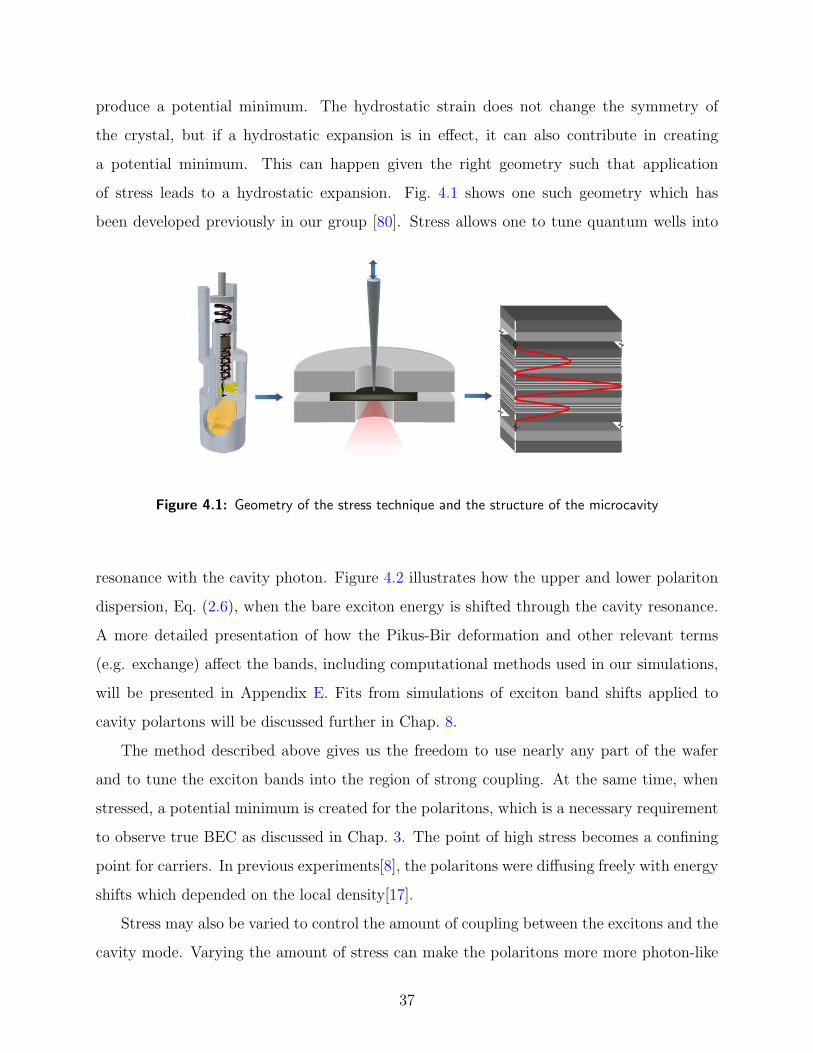
produce a potential minimum. The hydrostatic strain does not change the symmetry of

the crystal, but if a hydrostatic expansion is in effect, it can also contribute in creating

a potential minimum. This can happen given the right geometry such that application

of stress leads to a hydrostatic expansion. Fig. 4.1 shows one such geometry which has

been developed previously in our group [80]. Stress allows one to tune quantum wells into

Figure 4.1: Geometry of the stress technique and the structure of the microcavity

resonance with the cavity photon. Figure 4.2 illustrates how the upper and lower polariton

dispersion, Eq. (2.6), when the bare exciton energy is shifted through the cavity resonance.

A more detailed presentation of how the Pikus-Bir deformation and other relevant terms

(e.g. exchange) affect the bands, including computational methods used in our simulations,

will be presented in Appendix E. Fits from simulations of exciton band shifts applied to

cavity polartons will be discussed further in Chap. 8.

The method described above gives us the freedom to use nearly any part of the wafer

and to tune the exciton bands into the region of strong coupling. At the same time, when

stressed, a potential minimum is created for the polaritons, which is a necessary requirement

to observe true BEC as discussed in Chap. 3. The point of high stress becomes a confining

point for carriers. In previous experiments[8], the polaritons were diffusing freely with energy

shifts which depended on the local density[17].

Stress may also be varied to control the amount of coupling between the excitons and the

cavity mode. Varying the amount of stress can make the polaritons more more photon-like

37

or more exciton-like, as shown in Figure 4.2. As discussed earlier, controlling the amount of

coupling allows one to increase or decrease the lifetime of polaritons at will. Applying the

E

k||

E E

k||

k||

Figure 4.2: Different possible tunings with increasing stress. Left to Right: Negative, Zero, and Positivedetunings. Upper and Lower Polariton (Black Solid), Bare Exciton (Blue Dashed), Bare Cavity (RedDotted). Stress shifts the exciton state down while the cavity photon is essentially unchanged.

technique in practice is illustrated in Figure 4.1. The spring constant is inversely proportional

to the thickness of the sample. The thinner the sample the deeper and smaller the trap is.

While a deep and small profile is often desirable, there is a greater risk of breaking the sample

during handling. In Chap. 7, results are generated from a sample with 40 µm thickness. The

rest of the samples used in experiments have a 150 µm thickness . In Fig. 4.3, the sample

is stressed until the bare exciton energy is as close to the microcavity resonance as possible.

A force is applied on the back side of a 40 µm substrate with a rounded-tip pin with 50

µm or less tip radius. Figure 4.3 shows a typical profile of the the lower polariton potential

well created by stress. Directly under the stressor, the lower polariton branch has an energy

minimum which can be well fit by a harmonic potential [80, 37] U = 1/2γr2 where r is the

distance from the center of the trap and γ = 150 eV/cm2. This corresponds to a quantum

level spacing in the harmonic potential of hω0 = 0.037meV where ω0 =√γ/m is the natural

frequency and m is the effective mass equal to 8 × 10−5me. The continuum approximation

for the polariton states in the trap is valid here since this level spacing is much less than

kBT = 0.345meV at 4 K. Stress trapping allows theory to treat a quasi-equilibrium gas with

a known confining potential. This method opens a variety of possibilities and promise in the

area of microcavity research and BEC of polaritons.

38

313 353 393 433 473 513 5531.589

1.590

1.591

1.592

1.593

1.594

X [ m]

Ene

rgy

[eV

]

0

5.0E3

1.0E4

-120 -80 -40 0 40 80 120

Figure 4.3: Profile of the stress well created by 1.5N of force on the pin stressor. Sample excited withlaser defocused laser (722 nm ≈ 1.72 eV, 2.3 mWPump Power, ∼ 2 mm diameter) to view the wholestress well profile. Dashed line: Fit to a harmonicpotential.

4.2 CHARACTERISTICS OF A MICROCAVITY WITH A STRESS TRAP

We have already achieved active tuning of the polariton resonance of QW excitons in a

semiconductor microcavity using applied stress. Starting with a QW exciton energy higher

than the cavity photon mode, we used stress to reduce the exciton energy and bring it into

resonance with the photon mode. At the point of zero detuning, line narrowing and strong

increase of the photoluminescence are seen. By the same means, we create an in-plane

harmonic potential to trap the polaritons. In Chapter 7, we discuss drift of the polaritons

into this trap.

4.2.1 Photoluminescence and Reflectivity

Figures 4.4 and 4.5 show photoluminescence and reflectivity data for a sequence of increasing

stresses applied to this sample. The huge slope in energy of the lower polariton is due to the

spatial variation of the cavity length across the sample (see discussion in Chap. 2.4). The pin

stress point is chosen several millimeters to the right of the point of strongest coupling, where

the exciton energy is ∼ 20 meV higher than the photon energy. For the photoluminescence,

a helium-neon laser source (633 nm) is used to excite the sample off-resonantly, well above

the band gap, at θ = 12 incidence, and defocused to a spot size of several millimeters to

cover the entire region of observation. Photoluminescence emission collected normal to the

39

sample is directed to a spectrometer and captured with a Photometrics back-illuminated

CCD camera. For the sample reflectivity, a collimated light beam (750 nm−1000 nm) is

directed normal to the sample. The reflected light is also collected normal to the sample. A

mirror placed in the same plane as the sample is used to normalize the sample reflectance.

For all the experiments, the sample was maintained at the temperature of 4 K. At this

low temperature, no photoluminescence is seen from the upper polariton, as the polaritons

scatter to a lower energy state before recombination. Upper polariton emission for this

sample starts to appear at about 40 K.

Figure 4.4: Left: Luminescence spectrum as afunction of position on the sample, for various lev-els of force on the pin stressor, (a) unstressed, (b)0.75 N, (c) 1.50 N, (d) 2.25N, (e) 2.63 N, (f) 2.85N (white: minimum; black: maximum intensity).These images were created by illuminating the en-tire observed region (2.2 mm diameter) with a 5mW HeNe laser. Right: The corresponding re-flectivity (black: 0.0; white: 1.0). A harmonicpotential is clearly seen in both upper and lowerpolariton branches.

In addition to the energy shift of the bands, a striking increase of the photoluminescence

occurs, as seen in Figure 4.5. This is similar to the increase of photoluminescence at reso-

40

1.595 1.600 1.605 1.610 1.615 1.620 1.625

2.0x105

4.0x105

6.0x105

8.0x105

1.0x106

1.2x106

1.4x106

Force on Pin Stressor Unstressed 0.75 N 1.50 N 2.25 N 2.63 N 2.85 NIn

tens

ity [A

rb. U

nits

]

Energy [eV]

x10

15 meV

Ref

lect

ance

22 meV

15 meV

Figure 4.5: Top: Reflectivity at the bottom ofthe stress well, for a series of applied forces. Bot-tom: Photoluminescence emission of the lowerpolariton, taken with the HeNe excitation source(900 µW) focused (75 µm) at the bottom of thestress well.

nance seen by tuning of the resonance using a wedge of varying cavity thickness,[71] but the

increase in the present case is dramatic, a factor of about 100. The increase of the total pho-

toluminescence emitted from the front surface is consistent with an increase of the coupling

constant at resonance[71]. Consistent with the strong coupling, one can see in Figure 4.5 the

narrowing of the reflectivity spectra as the bare excitons and bare photon modes approach

resonance[23] during stress tuning.

4.2.2 Drift

Since there is an energy gradient for the polaritons, one expects that they will undergo drift.

Figure 4.6 shows spatially resolved photoluminescence when the laser is tightly focused and

moved to one side of the potential minimum in the lower polariton branch. Some polaritons

clearly live long enough to be observed over a distance of more than 100 µm, similar to what

was seen in earlier drift experiments[72] where an energy gradient is created by a wedge of

the cavity thickness. By determining the center of mass shift of the polariton luminescence

from Fig. 4.6, we measure the drift length ld to be 18 µm. From the measured drift length,

41

Figure 4.6: Spatially resolved photoluminescence for 2.85N applied force (white: minimum, black: maximum inten-sity) with the laser focused (75 µm FWHM) and shifted100 µm away from the center of the stress well. The pho-toluminescence is superposed on the reflectivity spectrum(gray) for the same conditions, to show the location of thewell.

we can estimate the relevant scattering time constant τsc. From classical gas kinetics, the

distance travelled by a particle due to a force is

ld = vd τ0 (4.2)

where vd =

(F

m

)τsc. (4.3)

From Fig. 4.6, F ≈ ∆U/∆x = 100 meV/cm. Using a polariton lifetime τ0 = 30 ps and

polariton mass m = 7 × 10−5 m0, Eq. (4.2) gives 24 ps for the relevant scattering time τsc.

This, however, is a shallow trap. In our experiments, the typical spring constant of the

trapping potential is around 150 eV/cm2 (refer to Fig. 4.3). Drift length can be an order of

magnitude longer, e.g. see Fig. 7.1.

From the deduced scattering time τsc = 24 ps, we can also calculate the diffusion length

lD. In two dimensions, the diffusion length is written as

lD =√Dτ0 (4.4)

where D = v2Dτsc =

2kBT

mτsc. (4.5)

At T = 16 K, the estimated diffusion length is equal to 70 µm. Normally, without a gra-

dient in energy, polaritons diffuse away from the excitation spot. With the stress potential,

42

polaritons drift toward the center of the trap where they remain concentrated. The increase

of the PL intensity seen in Figure 4.5 may be partly related to this feature. This is an

important feature of our system, since we can generate the polaritons with a laser that is

focused far from the center of the trap and watch them accumulate where there is no laser

excitation. This technique removes the ambiguity in determining if the pump laser is causing

the coherent effects. Later in Chap. 7, I shall present effects associated with spontaneous

Bose coherence in the trap with the pump on the side.

4.2.3 Evaporative Cooling Effect

-60 -40 -20 0 20 40 601.600

1.602

1.604

1.614

1.616

1.618

1.620

Ener

gy [e

V]

x [ m]

A

-60 -40 -20 0 20 40 600.45

0.50

0.55

0.60

0.65

0.70

0.75

0.80

Phot

on F

ract

ion

x [ m]

B

Figure 4.7: (A) Upper and lower polariton energies from photoluminescence and reflectivity spectra,when a force of 1.5 N on the pin stressor is applied to the sample. (B) Photon fraction of the lowerpolariton branch as a function of position in the trap, calculated from the polariton energies shown in(A) and the standard Hopfield coefficients, Eq. (2.5).

In real space, the exciton energy gets shifted down more where the center of the pin

is. In the center of the trap, the cavity photon states and the exciton states are strongly

coupled. Figure 4.7 shows that the polariton photon fraction increases as one moves away

from the center. The lower polariton photon fraction is much smaller in the center of the

well compared to the the regions away from it. This is good because at higher energies, far

from the center, the polariton is actually more photon-like and does not stay long in the

well. The mixing with the photon states leads to a decreased lifetime for high-energy states,

effectively leaving the cooler polariton gas in the trap [81] similar to an evaporative cooling

43

effect in trapped atomic gases[82, 83]. Naturally, this effect would only work if the polaritons

have long enough diffusion length to move through the whole trap. This is the case in our

experiments, where in some cases the polaritons move more than 50 µm. In principle, this

effect can be increased by the use of larger stress to positively detune the cavity so that the

polaritons are more than 50% exciton like at the center and become completely photon-like

away from the center. Unfortunately, no quantitative measurement of the lifetimes across

the stress well has yet been made.

44

5.0 OPTICAL METHODS

5.1 IMAGING AND SPECTROSCOPIC TECHNIQUES

Figure 5.1: Experimental setup for spectral and spatial imaging

The nature of the microcavity samples having distinct properties (e.g. coupling) at

different regions, and the technique of stressing requiring a precise knowledge of the stressor

point, necessitated a permanent imaging set-up to be in place for all measurements. Imaging

can be done normally using a lens to see the spatial profile of the polariton stress well. One

may also look at the luminescence at different energies and wave vectors using a fiber optic.

Signals are sent to a Photometrics Cascade512B back-illuminated CCD camera via an Acton

SpectraPro2300i spectrometer. The setup for doing imaging and spectral measurements is

shown on Figure 5.1. When taking images, the front slit is opened and the grating is rotated

to its zeroth order so that it is simply working as a mirror. The imaging spectrometer has

a grating with 1800 grooves/mm. The grating, in its zeroth order, is a poor mirror but our

45

samples emit more than enough light to compensate. The maximum spatial resolution of

the imaging setup is 8 µm, measured using an EdmundOptics USAF SQ Negative resolution

target. When taking spectral measurements, the spectrometer is set at its maximum spectral

resolution of 0.06 nm with the front slit opened to 40 µm. The light source used for calibrating

the spectral resolution was the diffuse reflection of a single-mode CW Ti-Sapphire laser at

771 nm which is around the spectral region of our polariton luminescence.

The sample is held inside a continuous helium-flow cryostat where it is kept at a low

temperature, usually around 4 K. For lower temperatures, a liquid helium immersion cryostat

maybe used. The sample may be excited using different sources. A continuous spectrum

of light from 750-1000 nm is used to take the reflectivity of the sample. A tunable laser

may be also used to pump the sample resonantly or non-resonantly at different angles.

The measurements presented were made with a MIRA 900 Ti-Saphire laser from Coherent.

Quasi-CW excitation was achieved using a NEOS acousto-optic modulator.

Figure 5.2: Experimental setup for angle-resolved measurements with a diffuser plate

Several techniques were developed for angle-resolved spectroscopy. One technique, uti-

lized particularly for low signal or low pump intensities, was collecting light emission from

the sample at different angles with a fiber bundle, as shown in Figure 5.1. For high-intensity

signals, a convenient method of taking angle-resolved measurements is by placing a diffuser

plate in front of the sample(see Fig. 5.2). The diffused light is then imaged on a spectrom-

eter for quantitative analysis. The advantage of the diffuser is that it provides information

simultaneously for both the horizontal and vertical components of the angle dependent PL

46

emission.

5.2 MEASURING COHERENCE WITH A MICHELSON

INTERFEROMETER

In BEC, coherence of the wave-like state extends over the whole extent of the condensed

entity. Coherence is measured by the correlation or the ability of two spatially and temporally

separated points of the wave to interfere.

Figure 5.3: Michelson interferometer setup for first order coherence measurements

To measure the first-order coherence of the polariton condensate, a Michelson interfer-

ometer was setup (See Fig. 5.3). Using a beam splitter, two arms of the interferometer

get identical copies of the polariton emission. Copies of the real image are projected onto

a CCD camera. The images can be overlapped spatially by tilting the mirror for one path

and temporally by changing the relative delays of the two paths. In effect, one end of the

condensate (A) is correlated with another end (B). The classical first-order correlation can

be written as

g(1) =〈E∗(x, t)E(x′, t′)〉〈E∗(x, t)〉〈E(x′, t′)〉

(5.1)

47

where E(x) is the electric field at x. The degree of coherence is measured by this average

correlation. Spatial coherence is oftentimes described in terms of visibility or the degree of

contrast of the interference pattern. Visibility is defined as (e.g. Ref. [84])

V =〈I(x, t)〉max − 〈I(x, t)〉min〈I(x, t)〉max + 〈I(x, t)〉min

(5.2)

The extremum intensity of the resulting overlapped signal can be written as

〈I(x, t)〉max = 〈I1〉+ 〈I2〉+ 2√〈I1〉〈I2〉|g(1)

12 | (5.3)

and

〈I(x, t)〉min = 〈I1〉+ 〈I2〉 − 2√〈I1〉〈I2〉|g(1)

12 | (5.4)

Hence,

V =2√〈I1〉〈I2〉

〈I1〉+ 〈I2〉|g(1)

12 | (5.5)

We see that, if the intensity of the two fields are equal, the visibility of the interference

pattern determines the first-order coherence. For infinitely coherent fields, the visibility

V = 1, and V = 0 for a totally incoherent source.

48

6.0 EXPERIMENTAL RESULTS WITH CW LASER PUMPING

Our earliest experiments with microcavity polaritons began with continuous-wave (CW)

laser pumping. It was a convenient setting to use being the default, stable operation of

our laser system, and was a natural choice after using CW mode in characterizing stressed

microcavities. With the CW mode, we can tune our laser for a wide range of energy (> 300

meV), necessary for pumping different frequencies of the polariton spectrum, while being able

maintaining pump intensities an order of magnitude greater than pump power thresholds

for BEC or photon lasing. More importantly it was necessary to be able see steady state

properties of the polariton systems. Later on, we realized that CW lasing introduces local

heating of the lattice leading to reduced drift, self-trapping and localization (see Chap. 6.3).

Quasi-CW pumping was later used to avoid this situation (see Chap. 7). Then, again, the

stability and power requirements needed to observe the two threshold behavior, attributed to

BEC and photon lasing threshold (see Chap. 6.5), prompted us to return to CW experiments.

6.1 STRESS AND POLARIZATION POWER SERIES

One reason why it is difficult to distinguish between photon lasing and BEC is that the

total carrier density in the case of the trapped polaritons in our experiments is not so much

different from the total carrier density in the case of weak coupling. Fig. 6.1 shows the gain

curves in our microcavity samples for four different conditions. Here the pump beam photon

energy is tuned to the edge of the stop band and is focused to 65 µm. The k‖ = 0 emission is

collected using a fiber and directed to the spectrometer and CCD camera. The blue inverted

triangles show the gain curve for the case when stress is applied to create a spatial trap for

49

1 10 100

1.12 N on Pin; Pump Center Unstressed Resonant 1.12 N on Pin; Pump Side 0.75 N on Pin; Pump Center

Tota

l. In

tens

ity 1

0% O

ffset

[Arb

. Uni

ts]

Pump Power [mW]

Figure 6.1: Photoluminescence intensity at k‖ =0 versus pump power at different amounts of forceon the pin stressors leading closer to a resonantstate and at different positions of the sample. Theplots are offset with respect to each other alongthe y-axis by 10%.

polaritons. At this stress point, the exciton and photon states are much closer to resonance

than before it was stressed. When the stress is relieved (black squares) the threshold for the

nonlinear gain, which corresponds to the onset of coherent behavior, increases dramatically.

There are two reasons for this. One is the decreased trapping, and the second is the fact

that releasing the stress takes the system farther from resonance, making the lower state

even more photon-like. To truly see the effect of the trap, one can move the excitation spot

to a region on the sample where the exciton and photon states are already in resonance

without need for stress tuning. This case is shown as the red circles in Fig. 6.1. This case

is comparable to the case of when the sample is excited on the side, far from the center of

a stress trap shown as the green triangles in Fig. 6.1. Clearly, the trap is playing a role,

since the threshold intensity for nonlinear gain with a stress trap close to resonance is less

than for the case of resonance with no stress trap. The threshold decreases further with

increasing stress. However, the difference in threshold is not more than a factor of three

or four. Also, small changes in the laser focus spot size and the absorption of the pump

laser due to the shift of the cavity reflectivity spectrum in the different cases of Fig. 6.1

lead to an uncertainty in the ratios of the densities by around 50%. The argument can be

made that if the carrier densities are comparable, the physics cannot be much different. On

first principles, of course, this need not be true. Many phase transitions occur which have

50

sensitive dependence on the total particle density. A Mott transition [65] from a system with

mostly excitons to one dominated by free-carrier plasma has been shown can occur with a

very sharply defined density[85]. Nevertheless, as will be shown in Chap. 6.5, we can directly

test whether the behavior of the coherent emission is different in the trapped and untrapped

case.

103

104

105

106

107

108

Tota

l Int

ensi

ty [A

rb. U

nits

] Total Intensity

0.2

0.3

0.4

0.5

0.6

0.7

0.8

FWH

M [m

eV]

FWHM

1 10 1000.0

0.1

0.2

0.3

0.4

0.5

0.6

(I max

-I min

)/(I m

ax+I

min

)

Pump Power [mW]

Polarization Degree

Figure 6.2: Top: Total intensity, Middle: Fullwidth at half maximum of the spectral intensity,and Bottom: degree of polarization as a functionof pump power the stressor setting that gives thelowest threshold

Figure 6.2 shows the total intensity at different pump powers with the corresponding

spectral width and for the case where the sample is pumped at the bottom of the stress well,

the degree of linear polarization of the polariton emission at k‖ = 0 was also measured. The

nonlinear threshold is defined as the pump power at the largest spectral width just before

it starts decreasing again. This coincides with the onset of nonlinear PL intensity and build

up of linear polarization. Above 30 mW pump power, one can observe a nonlinear increase

of intensity which becomes linear again at much higher pump power. Accordingly, there

51

is a dramatic narrowing of the spectral line width at the non-linear region, as shown by

the middle plot. Other groups [8, 14] have observed similar results. Note that in our case,

the pump beam is at the stop band edge with energy more than 120 meV higher than the

trapped lower polaritons. The point of exciting the polaritons at much higher energy is to

allow the polaritons to scatter and lose their coherence long before it accumulates in the

ground state, so that the coherence that occurs is not driven but spontaneous.

Below the nonlinear threshold, the photoluminescence emission appears to be completely

unpolarized. Above the threshold, one can observe build up of linear polarization. This is

an intriguing phenomenon because phase transitions such as BEC should be accompanied

by a form of ordering of the particles. If the polaritons are condensed in the ground state,

it should be described by a single wave function. One therefore expects a build-up of the

polarization of light. To make sure that the build up of polarization at the onset of the

threshold is not due to the laser’s polarization, the center of the stress well is pumped with a

circularly polarized laser. Figure 6.3 clearly shows that the polarization is not due to the laser

BA

0.00.20.40.60.81.0

0

30

6090

120

150

180

210

240270

300

330

0.00.20.40.60.81.0

1.1 mW 389 mW

0.00.20.40.60.81.0

0

30

6090

120

150

180

210

240270

300

330

0.00.20.40.60.81.0

0.97 mW 158 mW

Figure 6.3: Polarization below (red) and above (blue) threshold for different sample orientations.

because of the dramatic difference in polarization below and above threshold. In addition,

it is observed that the linear polarization follows approximately the general direction of the

[110] axis of the crystal. It may be deduced that the direction of polarization follows some

crystal axis, but the direction of polarization is not exactly fixed, it deviates around the [110]

axis from day to day. Analysis of the LP fine structure in Chap. 8 reveal that this maybe

due to the mixing of the light-hole and heavy-hole states with stress.

52

6.2 ANGLE-RESOLVED MEASUREMENTS

6.2.1 Angle-Resolved Power Series

At a given stress setting (see Fig. 4.3), the photoluminescence is collected for a set of an-

gles (−19 to 19) with respect to the normal of the sample for every power in a series of

powers. Below threshold, the PL is spectrally broad with minimal intensity. Above the ex-

citation threshold, one can clearly observe a distribution featured by a spectrally sharp and

intense peak formed at the center of the emission distribution. A blue shift and flattening

in momentum space is also observed. The blue shift is caused by renormalization due to

scattering between particles. The flattening in momentum space has been explained as due

to self-trapping [86] or localization of polaritons (see Chap. 6.3) resulting to the uncertainty

broadening (∆k∆x ≥ 1).

Figure 6.4: Angle resolved measurement below (2.3 mW), around (60 mW), and above threshold (139mW) pump power

Angle-resolved measurements of the photoluminescence intensity (Fig. 6.4) demonstrate

accumulation of particles in the ground state. In order to quantify that, we take represen-

tative samples of angle-resolved photoluminescence spectra and plot the relative occupation

number versus the peak energy for a given k-wavevector or angle (see Fig. 6.5). The rela-

tive occupation number is derived from the angular intensity distribution while taking into

account the lower polariton life time correction as a function of k (see Sec. 2.2.2). Below

12 mW pump power, the scattering mechanisms does not allow for particles to have enough

53

time to scatter to the ground state. Hence, neither a Maxwell-Boltzmann (MB) function nor

a Bose-Einstein (BE) function fits well to the angular intensity distribution. However, just

below the threshold (e.g. 37 mW), polaritons are able to thermalize possibly via polariton-

polariton scattering mechanisms. At this power, the occupation as a function of peak energy

at a given k-wavevector nicely fits the MB distribution with up to 98 percent confidence.

The temperature of the cloud measure from this distribution is about 16 K. At the threshold

(60 mW) the occupation fits the BE function by about 93 percent where temperature is fixed

to 16 K with as the fit parameter. For the BE fit at 60 mW, the chemical potential µ is at

-0.4 meV.

0.0 0.5 1.0 1.5 2.0 2.5 3.0 3.5

Occ

upan

cy (A

rb. U

nits

)

E-Emin (meV)

12 mW37 mW60 mW

x2

Figure 6.5: Occupation number from angle re-solved measurement at three different powers: lowpump power (12 mW), just below threshold (37mW), at threshold (60 mW). The occupation justbelow threshold (green circles) is well fit with a MBdistribution with temperature at 16 K. The occupa-tion at threshold (blue triangles) gives a 93% con-fidence for a BE fit with T = 16 K and µ = −0.4meV.

6.2.2 Occupation at Different Detuning and Stress

It is important to point out one other role that the stress trap is playing in these experiments.

As mentioned in a previous section, the bottleneck region is one of the features of the

microcavity that prevents scattering to the center of the trap. For an unstressed microcavity

(Fig. 6.6), one can see that the polaritons accumulate in the bottleneck region, corresponding

to the maxima of the hump in the occupation plot, since the lowest polariton state is mostly

photonic in character. In the stressed case, however, this hump or bottleneck accumulation

goes away, as shown by the upturn in occupation as the bottom of the stress well becomes

more excitonic. It could be argued that the more excitonic the polariton, the more gradual

54

0.0 0.5 1.0 1.5 2.0 2.5 3.0 3.5 4.00.1

1O

ccup

atio

n (A

rb. U

nits

)

E-Emin

(meV)

Photonic Resonant Excitonic

0.0 0.5 1.0 1.5 2.0 2.5 3.0 3.5 4.00.1

1

Occ

upat

ion

(Arb

. Uni

ts)

E-Emin

(meV)

MorePhotonic Photonic Resonant Excitonic

Figure 6.6: Comparison of the occupation at different detuning for the nonstressed and stressed case.Left: Occupation at different detuning as one moves across an unstressed sample through resonanceRight: Occupation at different detuning as one stresses the sample through resonance

the energy dispersion curves, making the bottleneck effect less of an issue.

To single out the effect of the trap from the polariton character (exciton-like ↔ photon-

like), one could move the stressor point to different regions away from resonance, regions

of negative detuning (δ = Eph − Eex < 0). If a position is more negatively detuned, more

stress is required to bring it into resonance with the cavity photon. Figure 6.7 is a series of

occupation from less negatively detuned to a more negatively detuned region of the sample

correspodingly increasing stress to bring it into resonance. This figure shows that at reso-

nance, increased stress helps populate the low energy states more efficiently. This suggest

that stress introduces a mechanism that helps polaritons overcome the bottleneck region

such that they are able to scatter to the ground state. Numerical models [38] indicate that

the applied stress may also play an indirect role in creating free carriers via ionization of

impurities due to the piezoelectric effect induced by stress. These free carriers may help

thermalize the polaritons to the lattice temperature.

55

0.0 0.5 1.0 1.5 2.0 2.5 3.0 3.5 4.00.1

1

Occ

upat

ion

(Arb

. Uni

ts)

E-Emin

(meV)

offset by 20%

increasing stress

Figure 6.7: Stressed to resonance with differentamounts of stress corresponding to different trapfrequencies ω0 =

√γ/m

Figure 6.8: Series of spectral pro-files at different pump powers TopRow: Pumping the unstressed res-onant sample (a) 1.17 mW, (b) 51mW, (c) 125 mW, Middle Row:Pumping the bottom of the stress well(d) 2.3 mW, (e) 49 mW, (f) 122 mWBottom Row: Pumping the side ofthe stress well (g) 2.3 mW, (h) 49mW, (i) 122 mW

56

6.3 REAL-SPACE DISTRIBUTION

Figure 6.8 shows real-space distribution of the energy profile for CW pumping at different

conditions. This series of images presents a comparison of the unstressed case in a region of

the sample with zero detuning of the exciton states relative to the cavity polariton states,

and in the case where there is a stress trap. In the nonstressed case, polaritons diffuse

freely from the excitation spot (see Fig. 6.8a-b). The spectrum is much wider and the

spatial size of the emission peak is significantly larger when there is no trapping. At higher

pump power, however, self trapping begins to dominate. One possible explanation[86] is

that lattice is heating creates a local minimum that traps the polaritons since increasing

lattice temperature red shifts the band gap[51, 50, 49]. High lattice temperatures at high

pump power may also explain the low diffusion constant, spatial narrowing, and spectral

broadening. This is one reason why we moved to the chopped-cw pump(see Chap. 7). In

addition, we find no evidence of build-up in linear polarization of the light emission in the

non-trapped case.

These figures (Fig. 6.8d-f) also show that the renormalization of the polariton energy due

to polariton-polariton repulsive interactions has the effect of flattening out the trap. Since

more polaritons accumulate in the center of the trap, the blue shift there will be largest,

tending to cancel out the effect of the external trapping potential. Therefore in the trap, the

potential felt by the polaritons is actually nearly flat. In the case of no trap, the polariton-

polariton repulsive interactions actually will tend to lead to a potential maximum at the

center of the laser excitation spot, which will have the effect of a pressure gradient causing

fast expansion of the polariton cloud. The relatively large effect of renormalization due to

particle-particle interactions in this system is the most significant way in which the theory

differs from that of trapped atoms.

Another interesting effect observed is the dramatic spatial narrowing of the as one in-

creases the pump power to create polaritons in the stress trap (see Fig. 6.9). The pump spot

has an average FWHM of about 65 µm. Intuitively, one might think that with more particles

and additional heating due to increased pump power that polaritons should fly apart but

instead they condense. This is consitent with the theory of BEC in a trap [87] that the

57

condensate should occupy the ground state of the trap, which is spacially compact. Above

the critical threshold, the spatial emission narrows to about 15 µm. This result is similar to

a thoeretical estimate[59] of the size condensate using our experimental parameters.

Figure 6.9: Two dimensional spatialprofiles for a series of powers

6.4 MEASUREMENT OF SPATIAL COHERENCE

We can also see direct evidence of coherence in the first-order correlation of the photolumi-

nescence, which is also seen in the work in CdTe structures [88]. Figure 6.10 shows images

produced by sending the spatially resolved photoluminescence through two arms of a Michel-

son interferometer, when the interferometer is slightly misaligned to create a double image in

which the left side of the image from one arm overlaps with the right side of the image from

the other arm1. Below the critical excitation density threshold, we cannot see any interfer-

ence fringes for any path difference of the two arms of the interferometer (Fig. 6.10A). Above

the critical density, fringes appear (Fig. 6.10B) across the two polariton condensates. The

faint fringes seen far away are not from the condensate but tails of a point spread function

due to the response of the imaging system to the condensate emission which is acting like

a point source. Figure 6.10C plots the visibility of the fringes, (Imax − Imin)/(Imax + Imin),

1See Sect. 5.2 for a review of coherence measurement using a Michelson interferometer

58

-24 -18 -12 -6 0 6 12 18

0.00

0.05

0.10

0.15

0.20

0.25

0.30

Vis

ibili

ty

Path Difference [ps]

Visibility Figure 6.10: False-color (blue = min, red =max) interference pattern through a slightly mis-aligned Michelson interferometer of the light emis-sion, with cw pump laser aimed at the center ofthe trap. a) laser power below threshold (cw aver-age power 37 mW); b) above threshold (73 mW).Total time delay of one path relative to the otherwas 1.56 ps. c) Visibility of the fringes as a func-tion of path difference under the same excitationconditions as (b). The solid line is a guide to theeye.

where Imax and Imin are the maximum and minimum intensity, respectively, as the path

length is varied under the same excitation conditions as in Fig. 6.10B. The visibility is never

100%, which is consistent with recent theoretical predictions [89] that the condensate frac-

tion of the polariton gas should be less than 50%. The coherence time increases from less

than 1 ps below the critical threshold to 8 to 10 ps above the critical threshold, which is

longer than the nominal lifetime of the polaritons in these structures of around 4 ps [9].

59

6.5 COMPARISON OF TRAPPED AND UNTRAPPED CASE

In earlier experiments showing nonlinearity of PL intensity, it was initially believed that

it is enough to show weak coupling if the emission line lies midway between the UP and

LP energy. Yet, even if that is not observed, photon lasing could still occur because of

the change in refraction index when increasing the carrier density so that the photon mode

is lower than midway between the UP and LP. This happens for most cases in untrapped

polaritons. Due to the refractive index change, lasing regime can actually occur at a much

lower energy than the uncoupled cavity or exciton mode[66]. This same effect also happens

in trapped polaritons but, as will be later shown, the BEC transition occurs at lower density

than the lasing transition. In this section we show the difference between the trapped and

untrapped case. Recent results[90] prove that stress traps play an important role in the

polariton quasiequilibrium condensation in GaAs microcavities.

To determine the point of strongest coupling and gauge the behavior of the polaritons

away from that point, it is necessary to monitor the shift of the lines relative to resonance.

Figure 6.11a shows the positions of the lines as a function of detuning across the sample.

The lines are well fit with a simple three-state coupling model (see Appendix A). The fit

functions correspond to the eigenvalues of the Hamiltonian matrixEHH1 0 Ω1

0 ELH1 Ω2

Ω1 Ω2 EPhot

(6.1)

with Ω1 = 7.55 meV, Ω2 = 6.0 meV, EHH1 = 1.616 eV, ELH1 = 1.646 eV, and Ephot shifting

with the wedge of the cavity as shown in Fig. 6.11.

The characteristics of the PL as a function of pump power in the nonstressed case, shown

in Fig. 6.12, clearly show only one transition occurring. Furthermore, the shift in peak energy

≈ 4 meV is very close to the Ω1 Rabi Splitting of 7.55 meV. Recall that the peak energy shift

does not have to be equal to the Rabi Splitting Ω1 since the cavity photon emission actually

red shifts as the cavity index of refraction changes with PL intensity [66]. It is reasonable

to claim that, with this amount of energy shift, the system is already in weak coupling.

Therefore, the transition can be associated with a standard photon lasing transition.

60

-20 -10 0 10 20 30

0.10.20.30.40.50.60.70.80.91.0

PL

Inte

nsity

(arb

. uni

ts)

-20 -10 0 10 20 30

-20 -10 0 10 20 300

20

40

60

80

100

120

140

CW

Pow

er a

t Thr

esho

ld (m

W)

Detuning = Eph - Eex (meV)

-20 -10 0 10 20 301.58

1.59

1.60

1.61

1.62

1.63

1.64

1.65

1.66

Ene

rgy

(eV

)

a)

b)

LH1

HH1

Phot

Figure 6.11: a) Squares: energy of the reflectionmaxima of the cavity as a function of detuning asthe cavity and exciton energy changes in energy dueto the gradient of the thickness in the sample. Thedata fits well to the model of coupled states dis-cussed in the text, using the exciton energies (HH1,HH2) and cavity photon energy (Phot) shown. Tri-angles: the photon emission energy as a functionof detuning when a laser excites the sample, withpower at the threshold for coherent effects. Thethreshold is defined as the point of maximum spec-tral line width before spectral narrowing occurs. Cir-cles: the photon emission energy when the laser ex-citation power is increased by a factor of 1.6 beyondthe threshold power. Circles, left axis: Photolu-minescence intensity of the lower polariton line asa function of detuning, for laser excitation densitywell below threshold (1.8 mW, with spot size 35 mi-crons). The intensity is maximum at resonance, δ= 0. Squares, right axis: The laser power neededto reach the threshold for coherent behavior (corre-sponding to the power used for the triangles in (a).)Laser spot size was 25 µm; laser photon energy was714 nm, at the absorption at the top edge of themicrocavity stop band.

To directly test whether the behavior of the coherent emission is different in the trapped

case, we can look at the behavior of the system as the detuning is varied, not by varying the

cavity length, as in Fig. 6.11, but by varying the exciton energy with stress. Figure 6.13a

shows the energy of the states as the stress is increased to change the detuning. The point

of resonance, i.e. the point of crossing of the bare cavity mode and the exciton mode, can

be identified in two ways. First, we fit the shifts of the lines with stress to the simple model

of coupled states as before. The parameters that coincide with the data or eigenvalues of

the Hamiltonian matrix are Ω1 = 7.5 meV, Ω2 = 6.0 meV, Ephot = 1.609 eV, and with EHH1

and ELH1 shifting with stress. The result is shown as the solid lines in Fig. 6.13a. Second,

we monitor the total photoluminescence intensity at very low pump intensity, as shown in

Fig. 6.13b. As in Fig. 6.11b, the photoluminescence has a maximum at the point of resonance

61

0

1

2

3

4

5

FH

WM

(meV

)

10 100

1.608

1.609

1.610

1.611

1.612

1.613

1.614

1.615

Pea

k E

nerg

y (e

V)

Pump Power (mW)

10 100101

102

103

104

Pea

k In

tens

ity (A

rb. U

nits

)

Pump Power (mW)Figure 6.12: a) Peak intensity of the emission fromthe lower polariton as a function of pump powerwhen the system is at zero detuning, when there isno stress trap - a location is chosen such that theexciton and cavity photon states are in resonance.b) Dots, left axis: peak photon energy of the emis-sion for the same conditions as (a). Solid line, rightaxis: the full width at half maximum of the emissionspectrum under the same conditions. The verticaldashed line is placed at the threshold pump powerdefined as the power at maximum FWHM just be-fore nonlinearity in PL occurs.

(though it has been shown that there is a fine structure very near to the resonance point

[71]). The FWHM of the PL intensity resonance around δ = 0 is about 10 meV in both cases

of Fig. 6.11b and Fig. 6.13b. As seen in Fig. 6.13a, when the pump power is increased to the

threshold for coherent effects, the energy of the emission shifts upward slightly, around 0.5

meV, but follows the lower polariton energy as it shifts lower with increasing stress, until

the detuning is around 4 meV. This clearly shows that the emission is still in the strong

coupling regime, since it follows the exciton shift very closely with stress detuning. For

detuning greater than 4 meV, the energy of the emission shifts up to near the bare cavity

photon energy (indicated by the dashed line in Fig. 6.13a). At this point it is reasonable to

assume that the system is no longer in strong coupling and the transition is a standard lasing

transition, red shifted relative to the bare cavity mode, as in Fig. 6.11a and in Ref. [66]. As

shown in Fig. 6.13b, to reach the standard lasing transition when the system is strongly

62

detuned, higher pump power, about a factor of two, must be used. This indicates that two

different transitions, polariton lasing (nonequilibrium polariton BEC) and standard lasing,

are occurring in the same sample. We therefore look to see both of these transitions occuring

at the same point in the microcavity sample by changing the pump intensity. Figure 6.14

shows that this indeed is the case.

Fig. 6.14a shows the intensity of the emission at different pump powers. The spectral

width is narrow, consistent with the low density and temperature of the polaritons. When the

density is increased, the spectral width first broadens (Fig. 6.14b), as expected for collision

broadening when the polaritons are at high enough density for substantial polariton-polariton

scattering. At the critical threshold for coherence, the spectrum narrows (Fig. 6.14b). Love

et al. [91] have recently argued that the intrinsic line width is much narrower, and the

observed spectral width here is primarily due to intensity fluctuations of the pump laser,

which is multimode in this case. This causes a fluctuating shift of the line position which

is recorded by a time-integrating detection system as a broadened line. In the experiments

of Love et al. [91], when an intensity-stabilized laser is used, very narrow line widths (∼

0.05 meV) and long coherence times (∼ 150 ps) are recorded for this type of polaritonic

transition. In addition, the shift in peak energy is less than 2 meV which is much smaller

compared to the Rabi Splitting of Ω1 = 7.5 meV. When the pump power is increased even

further (Fig. 6.14b), the emission broadens strongly and shifts strongly upward. This is

consistent with high-density effects such as phase-space filling and strong polariton-polariton

interaction, leading to breakdown of the pure polariton picture and onset of weak coupling

as discussed in Chap. 3.4 Finally, a second line narrowing is seen at the same spot in the

sample. This corresponds to standard lasing. At this point the shift in peak energy is more

than 4 meV comparable to the weak coupling regime in the unstressed case. There are

therefore two distinct transitions. The lower-power threshold can be identified with Bose

condensation of polaritons in the strong coupling limit, which occurs only when the trap

exists, while the higher threshold can be identified with standard lasing in the weak coupling

regime, and occurs in the unstressed sample as well as in the stressed sample when it is

detuned away from resonance. The trap plays an essential role in making the polariton

condensate transition possible. If there is no trap, only the lasing transition can be seen in

63

these samples. If there is a trap, both transitions can occur. Work in microcavities with

very high-quality reflection has also given indications of two distinct thresholds [92]. In that

case, the condensation is aided by longer lifetime of the polaritons, while in our case, the

condensation is aided by the trapping.

64

-6 -4 -2 0 2 4 6 8 100102030405060708090100110

Thr

esho

ld P

ump

Pow

er (m

W)

Detuning = Eph

- Eex

(meV)-6 -4 -2 0 2 4 6 8 10

Detuning = Eph

- Eex

(meV)

0.4

0.5

0.6

0.7

0.8

0.9

1.0

PL

Inte

nsity

(arb

. uni

ts)

LH1

HH1

Phot

-6 -4 -2 0 2 4 6 8 10

1.595

1.600

1.605

1.610

1.615

1.620

1.625

1.630

1.635

1.640

1.645

1.650

1.655

Ene

rgy

(eV

)

a)

b)

Figure 6.13: a) Squares: energy of the reflection maxima of the cavity as a function of detuning, whenstress is applied to vary the exciton energy while leaving the cavity photon energy unchanged. The dataare fits well to the model of coupled states discussed in the text, using the exciton energies (HH1, LH1)and cavity photon energy (Phot) shown. Circles: the photon emission energy as a function of detuningwhen a laser excites the sample, with power at the threshold for spectral narrowing. Inverted triangles:the photon emission energy when the laser excitation power is increased by a factor of 1.7 beyond thethreshold. Upright triangles: the photon emission energy when the laser excition power is increased bya factor of 2.5 beyond the threshold. b) Circles, left axis: Photoluminescence intensity of the lowerpolariton line as a function of detuning, for laser excitation density well below threshold (9 mW, withspot size 85 microns). Squares, right axis: The laser power needed to reach the threshold for coherentbehavior (corresponding to the power used for the circles in (a).) Laser spot size was 25 µm; laserphoton energy was 716 nm, at the absorption at the top edge of the microcavity stop band.

65

0

1

2

3

4

5

FW

HM

(meV

)

10 100

1.598

1.599

1.600

1.601

1.602

1.603

1.604

1.605

Pea

k E

nerg

y (m

eV)

Pump Power (mW)

10 100101

102

103

104

PL

Pea

k In

tens

ity (A

rb. U

nits

)

Figure 6.14: a) Peak intensity of the emission from the lower polariton as a function of pump powerwhen the system is at zero detuning, when the polaritons are generated in a stress trap under the sameconditions as those for Fig. 6.13. b) Dots, left axis: peak photon energy of the emission for the sameconditions as (a). Solid line, right axis: the full width at half maximum of the emission spectrum underthe same conditions. The acceptance angle for the PL detection was 0 ± 3. A different region ofthe sample was used, so that the lower polariton energy at zero detuning in this case is around 1.5984eV, as compared to 1.600 eV in Fig. 6.13. The acceptance angle for the PL detection was the sameas for Fig. 6.12. The vertical dashed (dotted) line is placed at the threshold pump power defined asthe power at maximum FWHM just before nonlinearity in PL occurs corresponding to a BEC (lasing)density threshold.

66

7.0 EXPERIMENTAL RESULTS WITH MODULATED QUASI-CW

PUMPING

While most of the experminents have been done with CW pumping, quasi-CW pumping

has its advantages. With a CW laser, the lattice is heated and the diffusion length of the

polaritons is much shorter (since polariton-phonon scattering is much faster). This means

that to get polaritons in the center of the trap in significant number, we need to focus the

laser on the center of the trap. However, there is an objection to pumping the center of the

well with the laser in that it raises the possibility that the most intense part of the laser

causes the effects that we see. With a modulated pump, less overall heating is going on

in the lattice. This turns out to be essential to allow long range motion of the polariton

gas. The disadvantage is that chopping the pump beam with an acousto-optic modulator for

quasi-CW output is not an efficient process. Given our present system, we are not able to

reach high enough density to observe the second threshold associated with ordinary photon

lasing.

7.1 DIFFUSION AND TRAPPING AT THE CENTER OF THE WELL

Figure 7.1 is a series of images of the polariton luminescence as the laser spot is moved

across the stress well. These polariton images are created by a pumping the edge of the stop

band (718 nm) with pump power above the threshold. One can clearly see that self-trapping

does not occur, but diffusion of polaritons gas to the center of the well. At very high pump

powers, self-trapping due to local lattice heating will eventually dominate. For these images,

the average laser power was 2.4 mW, for a circularly polarized, quasi-cw excitation with

67

Figure 7.1: Spatially-resolved spectra of the lightemission (external angle θ = 0 ± 5.2) from polari-tons in the microcavity structure, for three differentpositions of the laser. In (a), the polaritons areacreated on the left and flow to the right, in (b) theyare created in the trap, while in (c) they are createdon the right and flow to the left.

2.4% duty cycle at 1 kHz.

7.2 SIDE PUMPING POWER SERIES

In order to avoid ambiguity in regard to the possibility that the laser is causing the coherence

at the center of the well, we pumped the side of the well. What is shown in Figure 7.2 is

a series of images of polariton luminescence as the laser power is increased. Clearly, we see

diffusion then trapping at the center of the stress well.

If we pump the side of the well, and look at the luminescence normal to the sample or

at k|| = 0 just at the center of the well, we see still see the same nonlinear behavior above

a density threshold similar to what we have seen with CW pumping. We also see the same

spectral line narrowing. With pumping to the side, we have shown that the well has a huge

contribution to these effects. Below the threshold line (dashed line), the spectral width of

the photoluminescence emitted normal to the surface broadens with increasing density. Just

above the threshold line, the width of the photoluminescence spectrum drops sharply. At

68

Figure 7.2: Spatially-resolved spectra of the lightemission at (external angle θ = 0 ± 5.2) from po-laritons in the microcavity structure when the lasergenerates the polaritons on the left side of the trap,for three different laser powers (top t0 bottom): 0.4mW, 1.4 mW, and 2.4 mW.

the same time, we observe spatial contraction (Fig. 7.3b) of the polariton cloud by a factor

of three, down to the limit of our spatial imaging resolution (8 µm). As discussed in Chap. 6,

spatial contraction is also a telltale sign for condensation in a trap because the condensate

seeks the ground state of the system, which (in the case of a trapped gas) is a compact

state at the bottom of the trap. Below the critical density, in the normal state, the size of

the cloud is determined by a steady-state balance of the pumping by the exciting laser and

thermal diffusion; above the critical density, the size of the cloud is given by the size of the

ground state of the many-particle system. If interactions are neglected, the standard solution

of a harmonic oscillator gives a ground-state wave function with extent1 σ = 3.8 µm for our

parameters.. As discussed in Chap. 6.3, in the presence of particle-particle repulsion, the size

of the ground state will expand [87], but its size is still expected to be small compared to the

size of the cloud of thermal particles. This is a major difference between experiments with

1Note that the normalized ground state wavefunction for the harmonic oscillator is given by

Ψ0 =(mω0

hπ

) 14e−

mω0x2/h2 . (7.1)

It is easy to see that the wavefunction is a Gaussian function with standard deviation σ =√h/mw0.

69

and without traps: In a translationally invariant geometry, a superfluid will flow outward;

whereas, in a trap, it will flow inward.

0.1 1

1.596

1.600

1.604

1.608

1.612

1.616

UP Energy

LP Energy

Ene

rgy

[eV

]

Pump Power [mW]

8

10

12

14

16

18

20

22

24

Spa

tial F

WH

M [

m]

FWHM

0.55

0.60

0.65

0.70

0.75

0.80

0.85

FW

HM

[meV

]

k||=0 FWHM

104

105

106

Inte

nsity

[Arb

. Uni

ts]

k||=0 Intensity

a)

b)

c)

Figure 7.3: Data for polaritons in the center ofthe trap when the laser creates the polaritons onthe side of the trap, far from the center, similarto the conditions of Figs. 7.1 and 7.2. a) Solidblack squares: total photoluminescence intensityat k|| = 0 (external angle θ = 0 ± 1.0) as afunction of average excitation power, for quasi-cwexcitation with 2.4% duty cycle. Red dots: Fullwidth at half maximum of the emission spectrumat k|| = 0 under the same conditions. b) Fullwidth at half maximum of the spatial profile ofthe photoluminescence collected for external an-gle θ = 0±5.2 from the center of the trap underthe same conditions. c) Upper and lower polaritonenergies deduced from photoluminescence (lowerpolariton) and reflectivity (upper polariton) underthe same conditions. The vertical dashed line isplaced at the threshold pump power defined as thepower at maximum FWHM just before nonlinear-ity in PL occurs.

Monitoring the shift of both the upper and lower polariton states (Fig. 7.3) shows that

the system remains in the strong coupling regime during this transition. This is for the same

experimental conditions as Figs. 7.1 and 7.2. The red and blue curves correspond to the

upper and lower polariton lines at the center of the well. The LP shift in energy is only

about an meV at the nonlinear regime (dashed line) compared to a Rabi splitting of 7 meV.

70

7.3 SIDE-PUMPING REAL SPACE DISTRIBUTION

Figure 7.4 shows the spatial profile of the polariton cloud with the laser focused to one side of

the trap. The image of the profiles were obtained by projecting the PL emission of the cloud

onto a CCD camera. Although the polaritons are created on the side, the polariton cloud

drifts and remains centered on the bottom of the trap. As seen in Fig. 7.4A, at low pump

power, the cloud is centered approximately x = 50µm, y = 35µm. As the power is increased,

some of the polaritons remain in the region of the laser focus (Fig. 7.4B), at approximately

approximately x = 70 µm, y = 35 µm, due to the decreased diffusion constant. At the

critical threshold, Fig. 7.4C, a narrow peak appears at the trap center, much smaller than

the thermal size of the cloud at low density, while another peak remains at the excitation

laser spot. The peak the trap bottom continues to become sharper as the density is increased.

At even higher pump power, nonlinearity caused by the laser spot dominates, seen as the

most intense peaks in Fig. 7.4C and Fig. 7.4D. At these powers, 1.8 mW and 2.4 mW, normal

lasing is probably occuring at the laser spot. These results prove that the spatial narrowing

seen at the center of the trap can not come about simply by nonlinear gain of the laser

profile; the peak is due the collection of the polaritons in the ground state of the harmonic

potential of the trap.

7.4 ANGLE-RESOLVED MEASUREMENTS

A signature for BEC is evidenced by a bi-modal momentum distribution [93, 94, 95] of

the particles, which can be measured for polaritons by resolving the angular distribution of

the photoemission. This was seen in Fig. 6.5 for CW pumping at the center of the trap.

Pumping on the side of the well, however, creates a problem when taking angle-resolved

data. If one takes a spectra of the emission when pumping on the side, two distinct lines of

emissions will register in the spectrometer, one coming from where the sample is pumped and

another coming from the trapped polaritons at the center of the well. Due to this technical

difficulty, we had to pump the bottom of the well directly for angle-resolved measurements.

71

Figure 7.4: Two-dimensional spatial profile of the emission at k|| = 0 ± 5.2 for the average laserexcitation powers given, under the same conditions as Figs. 7.1 and 7.2. The profiles are normalized inintensity

Figure 7.5 shows a series of angle-resolved spectra under the same conditions as in Fig. 7.3,

but with the laser aimed at the center of the trap. A massive occupation in the ground

state is clearly seen as we go above the luminescence nonlinear threshold. This is seen as a

dramatic narrowing of both the in-plane momentum k|| and energy of the polaritons above

the critical threshold, while the blue shift due to interactions of the polaritons remains very

low. The contraction in momentum space that is simultaneous with contraction in real space

(Fig. 7.3B) does not contradict the uncertainty principle because both the spatial cloud size

and the momentum distribution are determined by thermal scattering when the polariton gas

is in the normal state, below the critical density threshold. Therefore, the total uncertainty

in the normal state ∆k||∆x (where ∆k|| is the uncertainty in the in-plane momentum and

∆x is the uncertainty in the in-plane position) is much larger than unity. The spatial size

of the condensate does imply a minimum width of the momentum peak at k|| = 0, which is

consistent with our data within our spatial (8 µm) and spectral resolution (0.12 eV) limits. In

the condensed state, ∆k∆x = (0.7× 104 cm−1)(15× 10−4 cm) = 10 > 1, which is consistent

72

with the uncertainty principle.

Figure 7.5: Angle-resolved light emission, for four different powers, under the same conditions asFig. 7.3 but with the laser aimed at the center of the trap. a) 0.05 mW (far below the thresholdexcitation density), b) 0.4 mW (just below the threshold); c) 0.6 mW (at the threshold); d) 0.8 mW(above the threshold). The false color scale is linear, with yellow=high and black = low.

Recall that these images give the dispersion relation of our lower polaritons (A fit to

Fig. 7.5 with a prabola gives the effective mass 7× 10−5m0 we have used). From these mea-

surements and the power correction factor (see Sect. 2.2.2), one can calculate the occupation

number. Figure 7.6 shows the relative number of polaritons per k|| state deduced from the

same data. The energy for each k|| is determined by the maximum of the measured spectrum

at each k||, in the same way as in Ref. [88]. Far below the critical density threshold, the

polariton distribution is completely nonthermal. Just below the critical density threshold, at

0.4 mW , the distribution is well fit by a Maxwell-Boltzmann distribution N(Ek) ∝ e−Ek/kBT

(where Ek is the particle energy, and N(Ek) is the number of particles per state at that en-

ergy), which corresponds to a straight line on this plot. Using the temperature T as a fitting

parameter we find that the effective temperature at equilibrium at around 97 K. This is much

higher than T = 16 K found for CW pumping. It is consitent with numerical models[38] that

show the polaritons are much more strongly coupled to the lattice when the temperature is

73

higher.

Above the critical threshold, there is a sharp increase in the number of polaritons near

k|| = 0. The high temperature of the Maxwell-Boltzmann fit below the critical density, which

is mirrored in the high-energy tails of the higher density N(Ek), indicates that the polariton

gas is not completely thermalized. As shown in recent theoretical works [93, 94, 95], the lack

of complete equilibrium does not prevent the polariton gas from undergoing a phase transition

to spontaneous coherence. The buildup of the particles at k|| = 0 is truly an effect of the

Bose statistics, but the entire range of energy cannot be fit to an equilibrium Bose-Einstein

distribution because the high kinetic energy particles (Ek > 1.5 meV) are constantly heated

by hot polaritons generated by the laser. This is also true of the occupation number data of

Ref. [88]. Steady-state quasiequilibrium theory [93, 94, 95] predicts a bimodal distribution

function N(Ek) (with a peak at k|| = 0 like that seen in Fig. 7.6, which corresponds to a

condensate) even when the system is not in complete equilibrium.

0 1 2 3 4

0.1

1

Occ

upat

ion

[Arb

. Uni

ts]

E-Emin [meV]

0.2 mW0.4 mW0.6 mW0.8 mW

Figure 7.6: Number of polaritons per k-state, de-duced from the light emission intensity as a func-tion of angle, for the same conditions as Fig. 7.5,for four laser powers as labeled. The straight lineis a fit to a Maxwell-Boltzmann distribution withT = 97 K.

7.5 POLARIZATION MEASUREMENTS

Similar to Ref. [88], we also see spontaneous buildup of linear polarization above the critical

density threshold (Fig. 7.7) as in the cw-pumping case. Also, the threshold intensity are the

74

0.1 10.00.10.20.30.40.50.60.70.80.91.0

Deg

ree

of P

olar

izat

ion

Pump Power [mW]

Polarization

0.5

0.6

0.7

0.8

0.9

1.0

1.1

FW

HM

[meV

] FWHM

103

104

105

106

107

Inte

nsity

[Arb

. Uni

ts]

Intensity

Figure 7.7: a) Red squares: Total photolumi-nescence intensity at k|| = 0 (external angle θ =0±1.0) as a function of average excitation power,for the same conditions as Fig. 7.5. Blue dots: Fullwidth at half maximum of the emission spectrumat k|| = 0 under the same conditions. b) Degreeof polarization (Imax−Imin)/(Imax+Imin) underthe same conditions.

same as the cw case if duty cycle is accounted for. Below the threshold, the light emission is

essentially unpolarized, which is not surprising because the pump light is circularly polarized

and the generated carriers must emit numerous phonons. Above the critical threshold, the

light becomes linearly polarized. We checked that this polarization is not related to the exci-

tation polarization or to the detection system by rotating the sample relative to the system.

We found that the linear polarization follows the sample orientation and is nearly aligned

with the [110] axis of the crystal, as in the CdTe experiments [88]. The polarization angle

also appears to depend weakly on the applied stress. Linear polarization has been predicted

[96] to be a direct result of spontaneous symmetry breaking in the polariton condensate

system; more recent theoretical work has shown that pinning along a crystal symmetry di-

rection is expected[97]. In Chap. 8, we will discuss this splitting of the linear polarization in

more detail. In general, when there is a condensate, any small term in the Hamiltonian that

breaks the degeneracy of the ground state will cause the condensate to jump into the lowest

energy state, even if the splitting is much less than kBT (refer to Chap. 3.3 for review).

75

8.0 EXPERIMENTAL MEASUREMENTS OF STRESS INDUCED

SPLITTING

A state splitting of up to 700 µeV is observed in the lower and upper polariton branches of

a stressed semiconductor microcavity polariton. The split states are linearly polarized and

orthogonal to each other. In addition, it is important to note that one of the state couples

to light better than the other, as seen by the difference in the Rabi splitting of the upper

and lower polaritons. A sample spectra is shown in Fig. 8.1.

1 . 5 9 0 1 . 5 9 5 1 . 6 0 0 1 . 6 0 50 . 9 8 80 . 9 9 00 . 9 9 20 . 9 9 40 . 9 9 60 . 9 9 81 . 0 0 01 . 0 0 2 L P

Refle

ctivity

E n e r g y ( e V )

9 0 D e g r e e s 1 8 0 D e g r e e s

1 5 . 4 m e V1 4 . 5 m e V

U P

Figure 8.1: An example of the reflectivity spectraof the polariton through a 90 and a 180 polarizerorientation. The spectra are taken 150 µm awayfrom the center of the stress well.

An example of the splitting of the lower polariton state in a line across the stress trap is

shown in Fig. 8.2(a). The difference in energy between two bright states is extracted from

photoluminescence measurements taken normal to the sample, and is plotted in Fig. 8.2(b).

The range of stress for the data of Fig. 8.2(b) are taken from close to zero detuning to

positive detuning (δ = Eph − Eex). Normal to the sample, the transverse electric (TE)

and transverse magnetic (TM) modes in the cavity are equivalent. Hence, the longitudinal-

transverse splitting of polaritons does not contribute to the splitting. The splitting could

arise from two possibilities. One is that it could be a direct effect of an energy splitting in the

76

degenerate bright exciton states (spin ±1) into two orthogonaly polarized radiative states.

Another possibility is that it could be due to a stress-induced birefringence in the microcavity

resulting to a splitting of the bare photon mode into two polarized states. However, the

photonic character is not enhanced in our case since the polariton becomes more exciton-

like with increasing stress[90, 81]. It is safe to assume that the splitting caused by a small

birefringence in the mirrors and cavity is not the dominant cause.

Exciton splitting due to exchange anisotropy is well studied in GaAs quantum wells and

microcavities[98, 99, 100, 101, 102, 103, 104]. However, known energy splittings of excitons

in quantum wells are typically only at most 200 µeV [99, 104, 101]. The mixing between

heavy-hole and light-hole excitons is negligible in the unstressed case since they are far apart

in energy (∼ 30 meV difference for 7 nm quantum wells). In our experiments [40], the stress

shifts the light-hole energy close to the heavy-hole energy making the mixing between the

two states an important parameter to consider.

- 4 0 0 - 3 0 0 - 2 0 0 - 1 0 0 0 1 0 0 2 0 0 3 0 0 4 0 0- 0 . 2- 0 . 10 . 00 . 10 . 20 . 30 . 40 . 50 . 60 . 7

LP Sp

litting

(meV

)

X A x i s ( m i c r o n s )

I n c r e a s i n g S t r e s s( b )

Figure 8.2: (a) An example of a lower polariton luminescence showing the splitting of the two brightstates across a stressed microcavity sample (4.3 N force on the pin stressor, see Refs. [37, 40] for thestressor geometry). The colored lines traces the points of maximum intensity. (b) Measured splittingof the between the lower polariton states with increasing force on the pin stressor (0 N, 0.2 N, 1.0 N,2.1 N, 3.2 N, and 4.3 N). The highest stress splitting corresponds to the difference (blue - red) of thecurves in (a).

The breaking of the degeneracy of the two bright excitonic states is the result of a lowering

of confinement symmetry that can be induced by external strain, piezoelectric fields inherent

77

and induced, and/or interface roughness possibly linked to the growth procedures[104, 105,

101]. This would mean a reduction of the symmetry of the QW from D2d to C2v [104].

Therefore, the [110] and [110] are no longer degenerate, splitting the exciton states into

orthogonal linearly polarized states. In D2d symmetry group, both the conduction spin

s = 1/2 states and valence j = ±3/2 states are represented by Γ6. The product gives

Γ6 ⊗ Γ6 = Γ1 ⊕ Γ2 ⊕ Γ5.

The representations Γ1 and Γ2 correspond to the dipole-inactive J = ±2 states and the Γ5

corresponds to the dipole-active J = ±1 states. When the symmetry is lowered to C2v, the

Γ5 becomes Γ2 ⊕ Γ4 which are optically-active x and y singlet states.

When the symmetry is lowered, it is natural to expect the exciton oscillator strength to

also be different along the two crystal axis orientations [104]. Each polarization would then

have a different Rabi splitting. In fact, the change in oscillator strength is a big factor in

creating these huge polariton splittings, up to 700 µeV seen in our experiments, since the

polariton splitting amplifies the spin splitting. The polariton energies for a given exciton

state is found by diagonalizing the matrix, Ei Ωi

Ωi Eph

, (8.1)

where Ωi is the radiative coupling for exciton eigenstate i, which depends on the relative

fraction of light-hole and heavy-hole exciton in the eigenstate.

The Hamiltonian that can split the degeneracy of the two bright states is the short-range

electron-hole exchange interaction between a hole with spin Sh and an electron with spin

Sh[106],

Hexch = −∑i=x,y,z

aiSh,iSe,i , (8.2)

where the a’s are the coupling constants. Anisotropy in the exchange interaction is enough

to split the degeneracy of the exciton states but it is not a necessary condition if there is a

strong mixing between the light- and heavy-hole excitons which is the case of our stressed

microcavity sample. Adding the Pikus-Bir deformation Hamiltonian, which determines the

78

shift of the bands with stress, to the exchange term and diagonalizing the resulting Hamilto-

nian matrix leads to a splitting of the exciton energy and a difference in the coupling strength

of the new states (see details in Appendix E). From the resulting exciton eigenstates and

their corresponding coupling strength to the cavity photon, we can solve for the energy of

new lower polariton states. For our fits to the data, we assume that the oscillator strength

of the pure J = ±1 heavy-hole exciton and the pure J = ±1 light-hole exciton remain

constant, but as the stress changes the relative fraction of eavy-hole and light-hole states in

each of the two new exciton eigenstates, the oscillator strength of each exciton state must

be recomputed.

The splitting in energies of the bright states using the Pikus-Bir plus exchange Hamilto-

nian for the exciton eigenstates, and then the polariton energy splitting using the calculated

light-hole and heavy-hole fractions, is compared to the data in Fig. 8.3(b). The data is well

fit using strain values, εxx, εyy, etc., for a line across the sample 25 µm off the center of

the pin stressor and in the direction of the [100] axis. The relevant parameteres used are

listed in Table 8.1. The Rabi splitting Ω is proportional to the square root of the calculated

oscillator strength |〈f |M |i〉|2, where the final states are the ±1 spin photons and the inital

states are the new eigenstates.

- 4 0 0 - 3 0 0 - 2 0 0 - 1 0 0 0 1 0 0 2 0 0 3 0 0 4 0 0

1 . 5 9 4

1 . 5 9 6

1 . 5 9 8

1 . 6 0 0

1 . 6 0 2

1 . 6 0 4

Energ

y (eV

)


( a )

- 4 0 0 - 3 0 0 - 2 0 0 - 1 0 0 0 1 0 0 2 0 0 3 0 0 4 0 0- 0 . 2- 0 . 10 . 00 . 10 . 20 . 30 . 40 . 50 . 60 . 7

LP Sp

litting

(meV

)


I n c r e a s i n g S t r e s s( b )

Figure 8.3: Splitting of the lower polariton with stress by adding the first exchange term to the Pikus-Bir Hamiltonian. (a) Colored lines show a sample fit to the photoluminescence of a stressed microcavitylower polariton from Fig. 8.2a (b) Fits to a series of stress splittings from Fig. 8.2b.

79

Table 8.1: Relevant parameters used for the Pikus-Bir and exchange term simulations shown in Fig. 8.3.

Hole diameter 1.25 mm

Pin diameter 25 µm

Relevant material parameters for GaAs/AlGaAs Ref. [78, 79]

Exchange coupling terms ax = ay 1.14 meV

az 0.84 meV

Bare heavy-hole radiative coupling Ωhh 7.55 meV

Bare light-hole radiative coupling Ωlh 6.0 meV

From the eigenvectors of the effective hamiltonian (Pikus-Bir plus exchange), we can

determine the direction of polarization of the exciton. One can write a general representation

of the exciton polarization as

P(x) =(A+ω

+ + A−ω−) , (8.3)

where A+(A−) are the amplitudes of right(left) circularly polarized light ω+(ω−) correspond-

ing to the sum of eigenvector elements with +1(-1) spin. If the magnitude of the amplitudes

are equal, r = |A−|/|A+| = 1, then the polarization is a 100% linear. For circular components

with equal amplitude, it is easy to show that

tan θ =A−ω

−

A+ω+=ω−

ω+(8.4)

θ =α

2(8.5)

where the circular polarization as a superposition of linear polarizations along the [100] and

[010] axes, ω± = 1√2

(ε1 ± iε2), α is the phase difference between the amplitudes, A−/A+ ∝

eiα, and θ is the direction of polarization with respect to the [100] axis. Calculating r and θ

from our simulations show that the polarization is nearly 100% linear and points effectively

in the [110] and the [110] directions, for lower polaritons near the center of the trap. In

our earlier paper [37], we presented evidence of optical anisotropy in which the emission is

80

linearly polarized and pinned to one of the [110] crystallographic axis above threshold. We

believe that this effect can be attributed to the anisotropy explained in this chapter.

These experiments provide an unusual degree of accuracy for the electron-hole exchange

parameters, because the microcavity makes the spin splitting of the different eigenstates

much larger than their line-widths. The sensitive dependence of the spin splitting on stress

also makes this a tool for measuring stress optically that does not depend on the intensity

of the lines. In addition, the splitting due to the stress trap removes the degeneracy of the

ground state. This may be a crucial factor in the reported observation of a Bose-Einstein

condensate in microcavity polaritons [19, 90], as compared to unstressed systems [92]. If

the ground state is degenerate, the total number of particles in the ground state is divided

equally among the degenerate states. This effectively increases the critical density threshold

for BEC.

81

9.0 CONCLUSION

From the beginning, this research sought to experimentally show proof of BEC in MCPs. The

first part consisted mainly of laying the ground work to make a polariton BEC theoretically

possible. That task included designing a MC sample that can support strong coupling

between excitons and photons such that an ensemble of stable polaritons could be studied.

It took several simulations, design, characterization (mostly reflectivity measurements), and

regrowing, which later on ended with the samples used in the experiments. The next task was

to create a potential trap for the polaritons that does not significantly alter its properties.

Stressing the sample, already having been tested and proven in the technique originally for

DQWs, was the reasonable choice and was ultimately convenient in effectively producing the

desired trap. After laying the ground work, the rest of the study proceeded in the search for

the signatures of polariton BEC.

Preliminary investigations have shown that the polaritons truly acted as a delocalized

gas, as demonstrated by its drift towards the stress-well minimum especially when a chopped

laser is used to avoid lattice heating. Further experiments have produced several compelling

evidence of Bose-Einstein condensation of polaritons. At the bottom of the trap, line nar-

rowing and non-linear increase of photoluminescence intensity were observed. Also a single,

spatially compact condensate gas of polaritons was formed in the trap analogous to the case

of atoms in a three-dimensional harmonic potential. Above critical density, we observed

massive occupation of polaritons in the ground state, spontaneous build-up of linear polar-

ization and macroscopic coherence of the condensate as seen in interference fringes all in

agreement with predictions. The dramatic transition of the system to a linearly polarized,

compact, coherent, and beamlike source is consistent with the picture of quasiequilibrium

condensation of polaritons.

82

Similar effects, however, were also observed in similar MC systems without traps. This

raised the question whether traps play a significant role at all in producing these effects. Our

experimental results prove that it does. Stressed samples showed a more efficient equilibra-

tion to the ground state. There are several aspects of the trap that have uniquely contributed

to the observation of BEC in our experments, namely: confinement of polaritons even when

created away from the trap center, change of the density of states, breaking of ground state

degeneracy, and the possibility of electron-polariton scattering due to free carriers by stress-

induced piezo-electric effect. More importantly, the use of stress traps has allowed us to

demonstrate a distinction between BEC and lasing. Comparison of the trapped and un-

trapped MCPs showed that the trapped case has two distinguishable transitions which can

be associated with pure photon lasing and BEC. For an identical sample, the untrapped

case showed only the photon lasing transition. The presence of two thresholds, one for BEC

and one for photon lasing, in the same trapped polariton system has so far been the most

incontrovertible evidence for achieving BEC in MCPs.

83

10.0 FUTURE DIRECTIONS

The study of Bose-Einstein condensation of polaritons is very much alive today, with a

flurry of exciting developments[107] that have been recently published. The most recent of

these is the demonstration of superfluid flow of a polariton condensates at long distances

while maintaining the population of these short-lived particles via parametric scattering[108].

Quantum vortices[109], another feature of superfluidity, have also been seen before that.

In addition, evidence of a condensed phase in the form of a Bogoliubov-like spectrum of

polariton condensates, as predicted by N. Bogoliubov for weakly interacting bosons[110],

has been presented[111]. Transition to a single macroscopic coherent state was also shown

over spatially delocalized disorder or potential traps[112]. Finally, some progress has been

made with room temperature polariton lasing using GaN microcavities[113], an encouraging

step toward the realization of polariton lasers as a new source of coherent light.

The results presented in this dissertation and elsewhere[37, 40, 90] have been a valu-

able contribution to the study of BEC of polaritons and macroscopic quantum phenomena

in general. Our experiments have allowed theory [81, 59, 38] to treat a quasi-equilibrium

gas with a known confining potential. Nevertheless, further manifestations of BEC may be

examined and fitted to theory. A key test is comparing the two-dimensional (kx and ky)

k-distribution of the polariton cloud below and above the condensate critical density. As

the trapping potential has some anisotropy to it, above threshold equilibration of the polari-

ton cloud should lead to an isotropic k-distribution of the condensate. By contrast, above

threshold, the condensate’s k-distribution must reflect the anisotropy of the trap. Such a

test has been started by my junior colleague and will be presented in a separate disserta-

tion. In addition, knowledge could be further gained in studying its dynamics. Ultrafast

time-resolved measurements will have to be made to understand the scattering mechanisms,

84

thermalization times, and evolution of the polaritons to completely understand the process

behind thermodynamic transitions that may occur. The system should be checked for a crit-

ical density threshold with its exact measure, its temperature dependence, and its agreement

to predictions of thermodynamic theories of weakly-interacting bosonic gases. The spectral

and spatial time-resolved distributions of the polaritons in the trap should be checked for

spectral and spatial peaks. Macroscopic coherence of polaritons in second order as well as

first order may also be investigated.

85

APPENDIX A

DEFINITION OF POLARITON HAMILTONIAN MATRIX

For two coupled quantum mechanical oscillators, we can write the Hamiltonian of the system

as

H = Epha†kak + Eexb

†kbk + Ω(a†kbk + b†kak) (A.1)

where a†k and b†k are the photon and exciton creation operators. The interaction term Ω is

called the Rabi splitting which determines the strength of dipole interaction between the

exciton and the light field. Note that

a†k|0〉 ≡ |ph〉 , 〈0|ak ≡ 〈ph|

b†k|0〉 ≡ |ex〉 , 〈0|bk ≡ 〈ex|.

Hence,

H = Eph|ph〉〈ph|+ Eex|ex〉〈ex|+ Ω(|ph〉〈ex|+ |ex〉〈ph|) (A.2)

and the matrix Hamiltonian is given by

H =

〈ex|H |ex〉〈ex|H |ph〉〈ph|H |ex〉〈ph|H |ph〉

=

Eex Ω

Ω Eph

. (A.3)

For the three state coupling mode,

H = Epha†kak + EHH1b

†kbk + ELH1c

†kck + Ω1(a†kbk + b†kak) + Ω2(a†kck + c†kak) (A.4)

86

where a†k, b†k, and c†k are the photon, heavy-hole exciton, and light-hole exciton creation

operators. The interaction term Ω1 (Ω2) are the coupling terms for the strength of dipole

interaction between the heavy-hole exciton (light-hole exciton) and the light field. Following

the same procedure used earlier for the two coupled quantum mechanical oscillators, we get

Hamiltonian matrix for the three state state coupling as

EHH1 0 Ω1

0 ELH1 Ω2

Ω1 Ω2 Eph

. (A.5)

87

APPENDIX B

QUANTUM THEORY OF EXCITON-POLARITONS

The theory of exciton-polaritons was introduced by J.J. Hopfield [20] in 1958. From that

time until the present, it has been refined and applied to various systems. The goal of this

appendix is to provide sufficient details for the reader to have a substantial understanding

of the theory. Here, I will follow and unify the work done by Hopfield [20], Kittel [114], and

Quattropani et. al. [115] using details that can be looked-up from well-known physics texts

by Jackson [116] and Klingshirn [117]. The reader may also follow derivations provided for

by D.W. Snoke in his recent book, see Ref. [53], which discusses closely related topics.

I will begin by solving a simple model for the dielectric function ε(ω). The model is of

an electron attached to a spring. Here, I will ignore the damping term and spatial dispersion

to have a simple but pedagogical illustration of polaritons. The equation of motion of the

oscillator is given by Newton’s second law.

m(x + ω′20 x) = −eE(x, t)

x + ω′20 x = − e

mE

p + ω′20 p = −e2

mE (B.1)

where p is the dipole moment, E is the driving field, and ω′0 is the resonant frequency. The

solution to this single electron oscillator is given by

p =e2

m(ω′20 − ω2)−1E (B.2)

88

The prefactor e2/m gives the coupling of the electromagnetic field to the oscillator in our sim-

ple model. The prime in ω′0 indicates corrections due to local fields and quantum mechanics

which I will later take into account.

For simplicity let us take N uncoupled oscillators. We then have the macroscopic polar-

ization given by

P = Np =Ne2

m(ω′20 − ω2)−1E (B.3)

Recall that

P = ε0χE andε(ω)

ε0= 1 + χ. (B.4)

Hence,

ε(ω)

ε0= 1 +

Ne2

ε0m(ω′20 − ω2)−1 (B.5)

For dense materials such as GaAs, the local field Eloc acting on the oscillators consists

of the external field E and the internal field Ei created by other dipoles. For a set N of

same kinds of molecules, P = N〈pmol〉 or in general P(x) =∑Ni〈pi〉 where pi is the dipole

moment of the ith type of molecule in the medium. Again for the same molecules

P = N〈pmol〉

〈pmol〉 = ε0γmolEloc

P = Nε0γmolEloc (B.6)

The molecular susceptibility γmol is given by the Clausius-Mossotti equation (see Jack-

son [116])

γmol =3

N

(ε(ω)/ε0 − 1

ε(ω)/ε0 + 2

)or

χe =γmol

1− 13Nγmol

(B.7)

89

The Clausius-Mossotti equation holds true for dense materials with large dielectric constants

such as GaAs. Plugging γmol from our derivation previously,

Nε0γmol =Ne2/m

(ω′20 − ω2)

Nε03

N

(ε(ω)/ε0 − 1

ε(ω)/ε0 + 2

)=

Ne2/m

(ω′20 − ω2)

ε(ω)/ε0 − 1

ε(ω)/ε0 + 2=

Ne2/3ε0m

(ω′20 − ω2)(B.8)

One can recover the original form of the dielectric function if we rewrite the resonant fre-

quency as a shifted eigenfrequency.

ω20 = ω′20 −

Ne2

3mε0

Hence,

ε(ω)/ε0 − 1

ε(ω)/ε0 + 2=

Ne2/3ε0m

(ω20 +Ne2

/3ε0m− ω2)

ε(ω)

ε0= 1 +

Ne2

ε0m(ω2

0 − ω2)−1 (B.9)

The resonant frequency ω0 is the observable quantity.

In quantum mechanics, the coupling term is given by the square of the allowed dipole

transition matrix element ∣∣HDif

∣∣2 =∣∣〈f |HD |i〉

∣∣2where i is the initial state, f is the final state and HD is the dipole operator ex. There are

various conventions for introducing the transition matrix element into the dielectric function.

I shall use use the convention as Klingshirn [117] used in his book. The a dimenstionless

quantity f =2mω′

0

he2|HD

ij |2 will be used to multiply the term Ne2m−1ε−10 . The product is often

called the oscillator strength f i.e.

f =2Nω′0ε0h|HD

ij |2

90

The dielectric function, in this notation, can then be written as

ε(ω)

ε0= 1 +

f

ω20 − ω2

. (B.10)

We shall see later that this oscillator strength f will show up in the coupling constant of

the interaction Hamiltonian of the polarization field and the photon field. Hopfield [20] in

his seminal paper on polaritons rewrites this dielectric function in this form

ε(ω)

ε0= 1 +

ω20β

ω20 − ω2

where f = ω20β. One can also arrive at this form of the dielectric function if we rewrite the

general equation of motion of the macroscopic polarization density P in the presence of a

driving electric field E as

P + ω20P = ε0ω

20βE(x, t) (B.11)

From this equation of motion, we could deduce the Lagrangian density for the polarization

field of this equation of motion. The Lagrangian can be written in two ways which are

equivalent and of course leads to the same equation of motion.

LP =1

2ε0ω20β

(P2 − ω2

0P2) + E ·P (B.12)

LP =1

2ε0ω20β

(P2 − ω2

0P2) + A · P (B.13)

Note that we can write E = −∇φ − A, B = ∇ × A and that ∇ · A = 0 in the Coulomb

gauge. Also for no source charge present, φ = 0. It is also important to keep in mind that

only the transverse modes couple with the photons. The longitudinal fields do not. Hence,

we can write A = AT + AL = AT . I will use the first form of the polarization Lagrangian,

Eq. (B.12), so that we could write the total Lagrangian for the photon field, polarization

field, and photon-polarization interaction as

Ltot =ε02

A2 − 1

2µ0

(∇×A)2 +1

2ε0ω20β

(P2 − ω2

0P2)− A ·P (B.14)

91

The dots in the vector fields represent partial derivatives in time. From the Lagrangian, the

total Hamiltonian density is written as,

Htot =3∑l=1

(∂LT∂Al

Al +∂LT∂Pl

Pl

)− LT

where

Ml =∂LT∂Al

= ε0Al − Pl

Πl =∂LT∂Pl

=P

ε0ω20β

(B.15)

Htot =1

2ε0M2 +

1

2µ0

(∇×A)2 +ε0ω

20β

2Π2 +

1

2ε0(1 +

1

β)P2 +

M ·Pε0

(B.16)

The vector field A is given by

A =

(h

ε0V

)1/2∑kλ

ελ(k)√2ωk

a†kλe

−ik·x + akλeik·x

(B.17)

and the canonical conjugate is given by M such that [A,M] = ih.

M = i

(hε0V

)1/2∑kλ

ελ(k)

√ωk2

a†kλe

−ik·x − akλeik·x

(B.18)

The first two terms of the total hamiltonian Htot gives the quantized photon energy.

Hphoton =

∫V

Hphoton =

∫V

1

2ε0M2 +

1

2µ0

(∇×A)2

= h∑kλ

ωk

(a†kλakλ +

1

2

)(B.19)

To get the equation above, we used the identity |∇ ×A|2 =∑α

|∇Aα|2 −∇ · [(A · ∇)A] −

(A · ∇)(∇ · A). The second term does not contribute to the integral and the last term is

zero in the Coulomb gauge.

The polarization term is less straightforward. There are two ways from where one can

define the field operators. One way is defining Π and P from

Hpol =ε0ω

20β

2Π2 +

1

2ε0βP2 (B.20)

92

so that

H = hω0

∑kλ

(b†kλbkλ +

1

2

). (B.21)

From this form of H we can deduce that

P =

(hε0βω0

2V

)1/2∑kλ

ελ(k)

b†kλe−ik·x + bkλe

ik·x

(B.22)

Π = i

(h

2ε0βω0V

)1/2∑kλ

ελ(k)

b†kλe−ik·x − bkλe

ik·x. (B.23)

It is easy to show that [P,Π] = ih. Note that we neglected spatial dispersion so that

the oscillators are uncoupled and resonate at frequency ω0. This is the path followed by

Hopfield [20] and Quattropani [115]. The extra term 12ε0

P2 from Eq. (B.15) will then have

the form

Hextra =

∫V

Hextra =

∫V

1

2ε0P2

=hβω0

4

∑kλ

(b†kλbkλ + bkλb

†kλ + b†kλb

†−kλ + bkλb−kλ

). (B.24)

The second way of defining P and Π is by following the procedure1 used by Kittel [114].

Kittel derived the polarization field operators using this term of the Hamiltonian density as

a whole.

Hpol =ε0ω

20β

2Π2 +

1

2ε0β(1 + β)P2 (B.25)

Thus our canonical polarization field operators P and Π become

P =

(hω0ε0β

2(1 + β)2V

)1/2∑kλ

ελ(k)

b†kλe−ik·x + bkλe

ik·x

(B.26)

Π = i

(h(1 + β)1/2

2ε0βω0V

)1/2∑kλ

ελ(k)

b†kλe−ik·x − bkλe

ik·x

(B.27)

1This is a more intuitive form and is easier when solving the eigenvalue problem. Another reason forfollowing Kittel is to get the total Hamiltonian in the usual form we often use for coupled two level systemsgiven by

Htot =∑

Epha†a +∑

Epolb†b + ih∑

Ω(b†a + h.c).

93

which gives

Hpol = hω0(1 + β)1/2∑kλ

(b†kλbkλ +

1

2

)(B.28)

Finally, we have the interaction term given by

Hinter =

∫V

M ·Pε0

(B.29)

Again, following Kittel’s notation, we change

(∑kλ

ελ(k)akλeik·x

)(∑k′λ′

ελ′(k′)bk′λ′eik′·x

)⇒

(∑kλ

a−kλbkλ

). (B.30)

Naturally, we also do the same for the complex conjugate. What happened here is that we

change k of the photon creation operators to −k and ελ(k)·ελ′(k′) = ελ(−k)·ελ′(k′) = δkk′δλλ′

(Note that the summation is from −k to k). Hence, we get the interaction term as

Hinter = i∑kλ

h√ωkω0

2

(β

(1 + β)1/2

)1/2 (a†kλbkλ − akλb

†kλ + a†−kλb

†kλ − a−kλbkλ

)(B.31)

Therefore, the total Hamiltonian becomes,

Htot = h∑kλ

ωk(

a†kλakλ +1

2

)+ ω0(1 + β)1/2

(b†kλbkλ +

1

2

)

+i

√ωkω0

2

(β

(1 + β)1/2

)1/2 (a†kλbkλ − akλb

†kλ + a†−kλb

†kλ − a−kλbkλ

) (B.32)

To diagonalize the Hamiltonian, we define a normal-mode annihilation operator

αk = wak + xbk + ya†−k + zb†−k (B.33)

where, as a normal-mode annihilation operator, it satisfies

[αk, H] = Ekαk (B.34)

94

The solution or expansion of the previous equation leads to a set of equations which can be

written in matrix form. Basically, it is an eigenvalue problem.A −iC 0 iC

iC B iC 0

0 iC −A −iC

iC 0 iC −B

w

x

y

z

= E

w

x

y

z

(B.35)

where

A = hωk, B = hω0(1 + β)1/2, C =h√ωkω0

2

(β

(1 + β)1/2

)1/2

.

The determinant of the matrix gives,

E4 − (A2 +B2)E2 + A2B2 − 4ABC2 = 0

E4 − E2(h2ω2k + h2ω2

0(1 + β)) + h2ω2kh

2ω20 = 0 (B.36)

Hence

h2ω2k

E2= 1 +

h2ω20β

h2ω20 − E2

(B.37)

If we write E = hω and replace ω0β = f we get back our original form of the dielectric

function

ε(ω)

ε0= n2 =

ω2k

ω2= 1 +

f

ω20 − ω2

(B.38)

We only take the positive solutions to the determinant, in other words, positive values of

energies. If we take the regime near resonance, we get the usual form of the ipper and lower

polariton derived from a simple two level system.

EUPLP

=Ephot + Epol

2±√

(Ephot − Epol)2 + Ω2

2(B.39)

where Ephot = hωk is the energy of the incident photon, Epol = hω0 is the energy of the

polarized particle and Ω =√ω2

0β =√f is the coupling constant. Actually, deriving this

form the original Eq. (B.36) is not trivial. The following provides the steps to arrive at

Eq. (B.39) from Eq. (B.36). We can rewrite Eq. (B.36) as

ω4 − bω2 + c = 0

95

where b = ω2k + ω2

0(1 + β) and c = ω2kω

20. I divided out h from E = hω so that it does not

have to carry h in every step.

ω =

√b

2±√b2 − 4c

2

Remember we are at close to resonance, ωk ≈ ω0. The term b2 − 4c would be a very small

number. Hence,

ω ≈√b

2± 1

2

√b2 − 4c

2b

=

√b

2± 1

2

√(b− 2

√c) (b+ 2

√c)

2b

Substituting back b and c we have,

√b

2=

√ω2k + ω2

0 + ω20β

2

=

√(ωk + ω0)2 − 2ωkω0 + ω2

0β

2

=

√((ωk + ω0)2

2

)(1− 2ωkω0 − βω2

0

(ω0 + ωk)2

)

≈

√((ωk + ω0)2

2

)(1− 2ω2

0 − βω20

4ω20

)

=

√((ωk + ω0)2

2

)(1− 2− β

4

)

≈

√((ωk + ω0)2

2

)(1− 1

2

)=

ωk + ω0

2

The assumption used here is that the coupling term β = f/ω0 is much smaller than 1.

The other term is easy enough.

b− 2√c = (ω0 − ωk)2 + βω2

0 = (ω0 − ωk)2 + Ω2

96

Finally,

b+ 2√c

2b=

1

2+

√c

b

=1

2+

ωkω0

ω2k + ω2

0 + βω20

≈ 1

2+

ω20

2ω20 + βω2

0

=1

2+

1

2 + β

≈ 1

Putting the h factor to the ω’s and plugging back everything together we get the usual form

of the upper and lower polariton equation.

EUPLP

=Ephot + Epol

2±√

(Ephot − Epol)2 + Ω2

2(B.40)

97

APPENDIX C

MICROCAVITY STRUCTURE

Figure C1: Layer structure of the semiconductormicrocavity sample used in all the experiments.

98

APPENDIX D

DENSITY OF STATES FOR A D-DIMENSIONAL POWER LAW TRAP

As pointed out by many authors (e.g. Ref. [57]), BEC is also possible for low-dimensions

in trapped geometries. Calculating the density of states for a given geometry is essential in

finding the critical density for BEC. The two dimensional case is, of course, more useful in

this dissertation but a general treatment of the density of states is handy when comparing

the different cases. Power law traps are considered here mainly because it is relevant in this

study. Anyhow, most traps can be approximated by a power law function near the minimum.

In addition, using power law traps lead to analytical solutions for the critical density. The

density of states will be solved semiclassically as traps commonly used in BEC are weakly

confining which means that the energy level spacing is much smaller than the thermal energy

of the particles.

The density of states is defined by ρ(E) = N ′(E) where N(E) is the number of states

with energy less than E. Semiclassically, apart from the constant in the denominator, the

integral

N(E) =

∫ ∫p2

2m+V (r)<E

ddr ddp

(2πh)d(D.1)

basically calculates the volume of a d-dimensional sphere of radius r(p). Hence, 1

1The author recomends Ref. [118] for those interested in following the algebra in solving this integral.

99

N(E) =1

(2πh)d

∫ r

0

ddr

∫ p

0

ddp

=1

(2πh)d

(2πd/2

Γ(d/2)

)2 ∫ ∫p2

2m+V (r)<E

drdp rd−1pd−1 (D.2)

where r and p are the maximum radius and momentum respectively. The maximum energy

E =p2

2m+ αrn

can be written in this form

1 =p2

2mE+α

Ern. (D.3)

To simplify the calculation, let

p =p2

2mEand r = r

(αE

)1/n

such that

1 = p2 + rn = p2 + (r2)n/2. (D.4)

N(E) =1

(2πh)d

(2πd/2

Γ(d/2)

)2 ∫ ∫p2+rn<1

drdp rd−1pd−1

= C

∫ ∫p2+rn<1

drdp rd−1pd−1

where C =1

(2πh)d

(2πd/2

Γ(d/2)

)21

αd/n(2m)d/2E(d/n+d/2)

=C

4

∫ ∫p2+rn<1

dr2dp2(r2)d/2−1(p2)d/2−1

100

Again, we can simplify the equation by introducing a change of variables x = r2 and y = p2.

Therefore,

N(E) =C

4

∫ 1

0

dxxd/2−1

∫ 1−xn/2

0

dyyd/2−1

=C

4

d

2

∫ 1

0

dxxd/2−1(1− xn/2)d/2

=C

4

d

2

2

n

Γ(1 + d/2)Γ(d/n)

Γ(1 + d/2 + d/n)

=(2m)d/2

(2hα1/n)d

(d

2

)Γ(d/n+ 1)

Γ(d/2)Γ(d/2 + d/n+ 1)Ed/2+d/n (D.5)

Finally, we can calculate for the density of states ρ(E) = N ′(E) for a d-dimensional

system in a power law potential.

ρ(E) =(2m)d/2

(2hα1/n)d

(d

2

)Γ(d/n+ 1)

Γ(d/2)Γ(d/2 + d/n)Ed/2+d/n−1 (D.6)

101

APPENDIX E

PIKUS-BIR HAMILTONIAN AND EXCHANGE TERM

The valence band energy shifts as a function of stresses is given by the Pikus-Bir deformation

Hamiltonian[77]:

HPB = a(εxx + εyy + εzz) + b[(J2x − J2/3)εxx + c.p.] +

2d√3

[1

2(JxJy + JyJx)εxy + c.p.

](E.1)

where a, b, and d are deformation potentials, εij’s are stress-tensor components, J ’s are

the angular momentum operators acting on the spin states of the valence band (m = 3/2,

1/2, −1/2, and −3/2), and c.p.’s correspond to cyclic permutations with respect to x, y, z.

Relevant material properties, e.g. deformation potentials and elastic constants, used in

our simulations are found in Refs. [78, 49, 79]. Acting on heavy-hole and light-hole ba-

sis,∣∣3

2, 3

2

⟩,∣∣3

2, 1

2

⟩,∣∣3

2,−1

2

⟩,∣∣3

2,−3

2

⟩, Eq. (E.1) gives the matrix form[78, 53] of the Pikus-Bir

Hamiltonian

HPB = −

P +Q −S R 0

−S∗ P −Q 0 R

R∗ 0 P −Q −S

0 R∗ S∗ P +Q

(E.2)

where

P = −av (εxx + εyy + εzz) , Q = − b2

(εxx + εyy − 2εzz) ,

R =

√3

2b (εxx − εyy)− idεxy , S = −d (εxz − iεyz) .

102

Diagonalizing this the matrix gives the shift of the valence band energies. The shift of the

conduction band is given simply by ∆Ec = ac (εxx + εyy + εzz).

Of course, to be able to diagonalize HPB through out the sample, we need the values

for the strain at different points on the sample as we stress it (see Refs. [80, 40]to stressor

geometry). The strain terms, εxx, εyy, etc., could be computed using programs that could

do finite-element analysis (e.g. ANSYS). Finite-element analysis numerically calculates the

displacements of a discretized mesh-representation of the sample using the constitutive rela-

tions of GaAs [53]. We begin by calculating the equilibrium displacement of the mesh points

by solving Newton’s law for continuous media. Following notation from Ref. [53], we have

∑j

∂σij∂xj

= ρui, (E.3)

where ρ is the density of GaAs and ui is the diplacement of a volume element in the i

direction. Combining this with Hooke’s law, σij =∑lm

Cijlmεlm, we get

ρui =∑jlm

Cijlm∂2ul

∂xj∂xm, (E.4)

where we define

εlm =1

2

(∂ul∂xm

+∂um∂xl

).

Eq. E.4 is discretized and applied to all points of the constructed mesh representation of

the sample when doing the actual simulation. A force on the stressor pin, for example,

corresponds to a displacement of the mesh points under the stressor. The right hand side

of Eq. E.4 calculates the force felt by the other mesh points, due the initial displacement.

The next iteration then is a displacement of each mesh point, in the same direction as the

force, with magnitude proportional to the force felt by each point. After the displacement,

the force is again calculated. The process repeats until equilibrium is reached. From the

equilibrium displacements (ui’s), one can calculate the strain terms, εxx, εyy, etc., that goes

into HPB.

103

- 8 0 0 - 6 0 0 - 4 0 0 - 2 0 0 0 2 0 0 4 0 0 6 0 0 8 0 01 . 5 3 0 51 . 5 3 1 01 . 5 3 1 51 . 5 3 2 01 . 5 3 2 51 . 5 3 3 01 . 5 3 3 51 . 5 3 4 0

Energ

y (eV

)

X ( m i c r o n s )

Figure E1: Example of a fit using strain simula-tions from ANSYS (red curve) on a single quantumwell energy of a stressed double quantum well (bluecurve, 0.7 N force on pin stressor), for an experi-ment similar to a work done previously [80]. Thefollowing book values (e.g. Ref. [78]) for the de-formation potentials of GaAs were used for thesefits: ac = −7.17 eV, av = 1.16 eV, b = −1.7 eV,d = −4.55 eV.

The Hamiltonian that can split the degeneracy of the two bright states is the short-range

electron-hole exchange interaction between a hole with spin Sh and an electron with spin

Sh[106].

Hexch = −∑i=x,y,z

aiSh,iSe,i (E.5)

where the a’s are the coupling constants. The first exchange term acting on hole-electron

basis,∣∣3

2

⟩|↑〉,

∣∣32

⟩|↓〉,

∣∣12

⟩|↑〉,

∣∣12

⟩|↓〉,

∣∣−12

⟩|↑〉,

∣∣−12

⟩|↓〉,

∣∣−32

⟩|↑〉,

∣∣−32

⟩|↓〉, gives

−

az

40 0 −(ax−ay)√

30 0 0 0

0 −az

4

−(ax+ay)√3

0 0 0 0 0

0 −(ax+ay)√3

az

120 0 2(ax−ay)

30 0

−(ax−ay)√3

0 0 −az

12

2(ax+ay)

30 0 0

0 0 0 2(ax+ay)

3−az

120 0 −(ax−ay)√

3

0 0 2(ax−ay)

30 0 az

12

−(ax+ay)√3

0

0 0 0 0 0 −(ax+ay)√3

−az

40

0 0 0 0 −(ax−ay)√3

0 0 az

4

(E.6)

The exchange term is added to the Pikus-Bir deformation matrix to account for the shift

of the bands due to both exchange and deformation. The Pikus-Bir Hamiltonian, acting in

104

the same basis state as the exchange, gives

HPB = −

P +Q 0 −S 0 R 0 0 0

0 P +Q 0 −S 0 R 0 0

−S∗ 0 P −Q 0 0 0 R 0

0 −S∗ 0 P −Q 0 0 0 R

R∗ 0 0 0 P −Q 0 S 0

0 R∗ 0 0 0 P −Q 0 S

0 0 R∗ 0 S∗ 0 P +Q 0

0 0 0 R∗ 0 S∗ 0 P +Q

. (E.7)

Diagonalizing HPB + Hexch at every point of a numerically discretized mesh of GaAs gives

you the shifted band energies at every point of the mesh, with stress.

The heavy hole excitons are those with the valence-band 3/2 states, while the light-hole

excitons are those with the valence-band 1/2 states. Only the states with J = 1 are bright

states, i.e. states∣∣3

2

⟩|↓〉,

∣∣−32

⟩|↑〉 for the heavy holes, and states

∣∣12

⟩|↑〉,

∣∣−12

⟩|↓〉 for the

light holes. The radiative oscillator strength for each eigenstate is proportional to |〈vac|p|i〉|2,

where

|i〉 = α1 |hh, 2〉+ α2 |hh, 1〉+ α3 |lh, 1〉+ α4 |lh, 0(a)〉

+α5 |lh, 0(b)〉+ α6 |lh,−1〉+ α7 |hh,−1〉+ α8 |hh,−2〉 (E.8)

is the eigenstate found in the above electron-hole basis. The matrix elements 〈vac|p|hh,±1〉 =

Mhh and 〈vac|p|lh,±1〉 = Mlh are fit parameters and the other matrix elements are zero.

105

APPENDIX F

TRANSFER MATRIX SIMULATION CODE

(* Description: modifying reflectivitytester.nb by rearranging the \

order of how the transfer and interface matrices are made. This uses \

Dr. D. W. Snoke’s method (from his book) of transfer matrices

TEST 2 uses the SPECS sent by Gregor Weihs WITH 30 Angs GaAs inserted \

in the GaAlAs layers

Sample 4_20_05.1 Specifications

This is the working version with Quantum Well resonance. Revised for \

normal incidence only.

*)

(*Remove["Global‘*"];Off[General::"spell"];*)

<< PhysicalConstants‘;

<< PlotLegends‘;

kb = (BoltzmannConstant/ElectronCharge )[[1]];

h = PlanckConstant[[1]];

c = SpeedOfLight[[1]];

106

q = ElectronCharge[[1]];

(* Test Parameters *)

(*

Center PThick

PThick =0.968;

*)(* Increasing thickness of each layer by some percent *)

T = 4.0; (* Temperature is 4K *)

(* \[Theta]=0*\[Pi]/180; Incoming wave angle *)

\[Lambda]C = 777.0*10^-9;

(* AlGaAs Refractive Index Model by Gehrsitz et. al.*)

(*

n[x_,\[Lambda]_,T_]:=Module[conv,E\[Lambda],AGaAs,E1GaAs,E\

\[CapitalGamma]GaAs,R,A,C1,E1,C0,E0,

conv=1/1.239856; (*For converting energy in terms of (\[Mu]m)^-1*)

E\[Lambda]=h*c/(q*\[Lambda])*conv;

AGaAs=5.9613+7.178*10^-4T-0.953*10^-6T^2;

E1GaAs=4.7171-3.237*10^-4T-1.358*10^-6T^2;

E\[CapitalGamma]GaAs=(1.5192+1.8*15.9*10^-3(1-Coth[(15.9*10^-3)/(2*kb*\

T)])+1.1*33.6*10^-3(1-Coth[(33.6*10^-3)/(2*kb*T)]))*conv;

R=((1-x)1.55*10^-3)/(0.724*10^-3-E\[Lambda]^2)+(x*2.61*10^-3)/(1.331*\

10^-3-E\[Lambda]^2);

A=AGaAs-16.159*x+43.511*x^2-71.317*x^3+57.535*x^4-17.451*x^5;

C1=21.5647+113.74*x-122.5*x^2+108.401x^3-47.318*x^4;

E1=E1GaAs+11.006*x-3.08*x^2;

C0=(50.535-150.7*x-62.209*x^2+797.16*x^3-1125*x^4+503.79*x^5)^(-1);

E0=E\[CapitalGamma]GaAs+1.1308*x+0.1436*x^2;

107

Sqrt[A+C0/(E0^2-E\[Lambda]^2)+C1/(E1-E\[Lambda]^2)+R]

]

*)

(* AlGaAs Refractive Index Model by Afromowitz for Room Temperature \

Measurements ONLY *)

(*

n[x_,\[Lambda]_, T_]:=Module[E\[Lambda],EO,Ed,E\[CapitalGamma],Ef,\

\[Eta],M1, M3,\[Chi] ,

E\[Lambda]=h*c/(q*\[Lambda]);

E0=3.65 + 0.871*x + 0.179*x^2;

Ed = 36.1 - 2.45*x;

E\[CapitalGamma]=1.424 + 1.266 *x + 0.26*x^2;

Ef=Sqrt[2.0*E0^2-E\[CapitalGamma]^2];

\[Eta] = (\[Pi] * Ed)/(2.0*E0^3*(E0^2-E\[CapitalGamma]^2));

M1 = \[Eta]/(2.0*\[Pi])*(Ef^4-E\[CapitalGamma]^4);

M3 = \[Eta]/\[Pi]*(Ef^2-E\[CapitalGamma]^2);

\[Chi]= M1 +M3*E\[Lambda]^2+\[Eta]/\[Pi]*E\[Lambda]^4*Log[(Ef^2-E\

\[Lambda]^2)/(E\[CapitalGamma]^2-E\[Lambda]^2)];

Sqrt[\[Chi]+1.0]

]

*)

(*N for quantum Well Resonance*)

nGaAsRes[\[Lambda]_, T_, Ex_, f_] :=

Module[ E\[Lambda], ExEn, er, ei, n, k, \[CapitalGamma],

E\[Lambda] = 1000*h*c/(q*\[Lambda]);(*the units is in meV*)

ExEn = (1000.0*h*c/(q*Ex*10^-9));

108

(*** Modified indices ***)

(*f=0.00625;*)

\[CapitalGamma] = 0.2; (*units of meV*)

er = 12.96 + (

f*ExEn^2*(ExEn^2 - E\[Lambda]^2))/((ExEn^2 -

E\[Lambda]^2)^2 + (\[CapitalGamma]*E\[Lambda])^2);

ei = (f*ExEn^2*\[CapitalGamma]*

E\[Lambda])/((ExEn^2 - E\[Lambda]^2)^2 + (\[CapitalGamma]*

E\[Lambda])^2);

n = 1/Sqrt[2]*((er^2 + ei^2)^(1/2) + er)^(1/2);

k = 1/Sqrt[2]*((er^2 + ei^2)^(1/2) - er)^(1/2);

n + \[ImaginaryI]*k

]

(* Jackson Method *)

Reflectivity[\[Lambda]_, nlist_, dlist_] :=

Block[layer, kmz, \[CapitalDelta], Dm, Pm, Transfer,

layer = Length[nlist];

(*ky=2\[Pi]*nlist[[1]]/\[Lambda] *Sin[\[Theta]];*)

(*kmz[nm_]:=Sqrt[(2\[Pi]*nm/\[Lambda])^2-ky^2];*)

kmz[nm_] := Sqrt[(2 \[Pi]*nm/\[Lambda])^2];

\[CapitalDelta][nm_, nm1_] := kmz[nm]/kmz[nm1];

Dm[nm_, nm1_] := (

1 + \[CapitalDelta][nm, nm1], 1 - \[CapitalDelta][nm, nm1],

1 - \[CapitalDelta][nm, nm1], 1 + \[CapitalDelta][nm, nm1]

)/2;

Pm[nm_, dm_] := (

109

Exp[\[ImaginaryJ]*kmz[nm]*dm], 0,

0, Exp[-\[ImaginaryJ]*kmz[nm]*dm]

);

Transfer = IdentityMatrix[2];

Transfer =

Dm[nlist[[1]], nlist[[2]]].Pm[nlist[[1]], nlist[[1]]].Transfer;

Do[

Transfer =

Dm[nlist[[q]], nlist[[q + 1]]] .Pm[nlist[[q]],

dlist[[q]]].Transfer

, q, 2, layer - 1];

(Abs[Transfer[[2, 1]]]/Abs[Transfer[[2, 2]]])^2

]

SetDirectory[

"C:\\Documents and \

Settings\\Administrator\\Desktop\\RyanTempFile"];

(*ExList = Import["mar13_1DeducedExlPixel46-465.DAT","TSV"];*)

Clear[\[Lambda]];

(*range=\[Lambda],765.0*10^-9,778.0*10^-9,0.5*10^-9; (* Wavelength \

range and increment *)

\[Lambda]list=Table[\[Lambda],Evaluate[range]]; *)

\[Lambda]list = Table[764.986 + 0.0140196*i, i, 929]*10^-9;

(* Variables for the excitong splitting fit from ArchiveJournal...

110

13Mar08_ExcitonSplittingFunction *)

xc = 256.9533;

A1 = 0.05;

A2 = -0.02376;

w1 = 156.37108;

w2 = 44.27311;

(* Difference in energy of the two stressed induced exciton states *)

ExDiff =

Table[0.00036 + (A1/(w1*Sqrt[Pi/2]))*

Exp[-2*((x - xc)/w1)^2] + (A2/(w2*Sqrt[Pi/2]))*

Exp[-2*((x - xc)/w2)^2], x, 46, 465, 1]*1000;

PThick = Table[0.966 + (45 + i - 50)*0.0016/500 , i, 420];

R = ; (* The reflectivity list *)

TopMirror = ;

BotMirror = ;

(*layer=105;*)

(*I Moved the Thickness List Here So That The Program Goes Faster*)

LAir = 4*\[Lambda]C*10^9/4;

dlist = LAir, 57.94;

Do[dlist = Join[dlist, 67.22, 57.94], 16];

dlist = Join[dlist, 44.22];


dlist = Join[dlist, 32.34, 3.0, 43.35, 7.00];


dlist = Join[dlist, 43.35, 3.0, 32.34];

111



Do[dlist = Join[dlist, 54.78, 3.0, 67.22], 20];


LGaAs = 5*\[Lambda]C*10^9/(4*n00);

dlist = Append[dlist, LGaAs];

dlist = dlist*1.0*10^-9;

(*****************************************************************)

(* if the values of n20 = 3.6, n100 = 3.08, and n00 = 3.65 , it came \

from S.Pau et al., Phys. Rev. B., Vol. 51, No. 20 1995*)

(* Values of the refractive indices at 777 nm and 4 Kelvin using \

Gerhsitz et. al.

Here I made them constant around the region of interest just to move \

the simulation faster *)

n20 = 3.45078;(* Refractive index of Subscript[Al, \

0.20]Subscript[Ga, 0.80]As *)

n100 = 2.97045;(* Refractive index of AlAs *)

n00 = 3.58944; (* Refractive index of GaAs *)

(*****************************************************************)

(* Building the refractive index and the thickness lists *)

(* First layer is air, second is AlGaAs *)

TopMirror = 1.0, n20;

(* LAir=4*\[Lambda]C*10^9/4;

dlist=LAir,57.94; *)

(* Top DBR 16 Layers AlAs-Subscript[Al, 0.20]Subscript[Ga, 0.80]As *)

Do[TopMirror = Join[TopMirror, n100, n20], 16];

112

(*Do[dlist=Join[dlist,67.22,57.94],16]; *)

(* Spacer *)

TopMirror = Join[TopMirror, n100];

(*dlist=Join[dlist,44.22]; *)

(***

.

.

.

***)

(* Spacer *)

BotMirror = n100;

(*dlist=Join[dlist, 44.42];*)

(* Bottom DBR 20 Layers Subscript[Al, 0.20]Subscript[Ga, \

0.80]As-GaAs-AlAs *)

Do[BotMirror = Join[BotMirror, n20, n00, n100], 20];

(*Do[dlist=Join[dlist,54.78,3.0,67.22],20];*)

(* The last layer is the bulk GaAs *)

BotMirror = Join[BotMirror, n00];

(*dlist=Join[dlist,700.0]; *)

(* GaAs Substrate *)

BotMirror = Join[BotMirror, n00];

(* LGaAs =5*\[Lambda]C*10^9/(4*n00);

dlist=Append[dlist,LGaAs];

113

dlist=dlist*1.0*10^-9*PThick; *)

(*****************************************************************)

(*n20=n[0.20,\[Lambda],T]; (*Refractive index of Subscript[Al, \

0.20]Subscript[Ga, 0.80]As *)

n100= n[1.0,\[Lambda],T]; (*Refractive index of AlAs *)

n00=n[0.0,\[Lambda],T]; (* Refractive index of GaAs *) *)

nQW = 2; (*Just for initialization *)

nlist = TopMirror;

(* 4 Quantum wells *)

Do[nlist = Join[nlist, nQW, n100], 4];


(* Spacer *)

nlist = Join[nlist, n20, n00, n100, nQW];

(*dlist=Join[dlist,32.34,3.0,43.35, 7.00]; *)


Do[nlist = Join[nlist, n100, nQW], 3];


(* Spacer *)

nlist = Join[nlist, n100, n00, n20];

(*dlist=Join[dlist,43.35,3.0, 32.34]; *)


Do[nlist = Join[nlist, n100, nQW], 4];


114

nlist = Join[nlist, BotMirror];

y0 = 767.19055;

mslope = 0.00076;

A1 = 1142.08324;

w1 = 205.39376;

xc = 209.75365;

A2 = 2.1992;

w2 = 26.94719;

For [FileNum = 0, FileNum < 6, FileNum = FileNum + 1,

coup = 0.00600;

RSeparated1 = ;

RSeparated2 = ;

ExList =

Table[y0 + 0.0015*0.25*FileNum*y0 + mslope*x +

0.20*FileNum*(2*A1*w1/Pi/(4*(x - xc)^2 + w1^2) +

A2*Exp[-((x - xc)/w2)^2]), x, 1, 420, 1];

For[ctr = 0, ctr < 2, ctr++,

coup = coup + ctr*0.0001*FileNum/5.0;

Ex = ExList + ctr*0.20*FileNum*ExDiff; (*

Splitting of the Exciton changes with stress *)

(*For[m=1,m<Length[\[Lambda]list]+1,m=m+40,*)

For[m = 600, m < 900 + 1, m = m + 1,

(*If [m==200, m =650]; (*Skip areas with no features*) *)

\[Lambda] = \[Lambda]list[[m]];

115

For[YPix = 1, YPix < 421, YPix = YPix + 1,

nQW = nGaAsRes[\[Lambda], T, Ex[[YPix]], coup];

(*Quantum Wells*)

nlist[[36]] = nQW;

nlist[[38]] = nQW;

nlist[[40]] = nQW;

nlist[[42]] = nQW;

nlist[[47]] = nQW;

nlist[[49]] = nQW;

nlist[[51]] = nQW;

nlist[[53]] = nQW;

nlist[[58]] = nQW;

nlist[[60]] = nQW;

nlist[[62]] = nQW;

nlist[[64]] = nQW;

(*PThick=0.967+ (45+YPix-50)*0.002/

410;*) (*Center at YPix 255 Corresponding to PThick = 0.968*)

(*R=Append[R,\[Lambda]*10^9, YPix,

Reflectivity[\[Lambda],\[Theta],nlist,dlist*PThick]];*)

R =

Append[R,

Reflectivity[\[Lambda], nlist, dlist*PThick[[YPix]] ]];

];

];

If[RSeparated1 == , RSeparated1 = R, RSeparated2 = R];

116

R = ;

];

RSeparated1 = Partition[RSeparated1, 420];

RSeparated2 = Partition[RSeparated2, 420];

Export["aug07_Sep1" <> "Stress" <> ToString[FileNum] <> "Ver9.DAT",

Transpose[RSeparated1], "TSV"];

Export["aug07_Sep2" <> "Stress" <> ToString[FileNum] <> "Ver9.DAT",

Transpose[RSeparated2], "TSV"];

];

(*SetDirectory["C:\\temp\\ArchiveJournal\\25Sep2008\\13Mar08"];

RSeparated1 = Import["mar13_Separated1Stress1.DAT","TSV"];

RSeparated2 = Import["mar13_Separated2Stress1.DAT","TSV"];*)

(*Animate[MatrixPlot[Sin[a]^2*Transpose[RSeparated2]+Cos[a]^2*\

Transpose[RSeparated1],ColorFunction->"GrayTones", \

PlotRange->Automatic,100,150,0,1.05],a,0,Pi]*)

(*Animate[MatrixPlot[Sin[a]^2*Transpose[RSeparated2]+Cos[a]^2*\

Transpose[RSeparated1],ColorFunction->"Rainbow", \

PlotRange->Automatic,20,80,Automatic],a,0,Pi]*)

(*MatrixPlot[(Transpose[RSeparated2]+Transpose[RSeparated1])/2,\

ColorFunction->"GrayTones", \

PlotRange->Automatic,140,160,0,1.05]*)

(*Animate[ListPlot[RDat[[1,All]],Sin[a]^2*RDat[[2,All]]+Cos[a]^2*\

RDat[[3,All]], Joined->True, PlotRange \

->Automatic,0,1.01],a,0,Pi] *)

117

(*ListDensityPlot[RDat,InterpolationOrder->3,ColorFunction->\

"GrayTones", PlotRange->Automatic,1,512,0,1.05 , AspectRatio -> \

0.551]*)

(*<<Graphics‘Animation‘

ShowAnimation[Table[ListDensityPlot[Sin[a]^2*RSeparated1+Cos[a]^2*\

RSeparted2,InterpolationOrder->3,ColorFunction->"GrayTones", \

PlotRange->Automatic,Automatic,0,1.05 ],a,0,Pi]]*)

118

APPENDIX G

MATLAB CODE FOR STRESS ANALYSIS

G.1 FUNCTION FOR PIKUS-BIR AND EXCHANGE CALCULATION

function StressExchangeUsingANSYSdata(StressOn, xf, yf, zf, u1 , u2, v1,

v2, w1, w2)

global StrainDat Emat ExchE OscStrength1 OscStrength2 HydroTerm vcenter

vside1 SimXaxis exx eyy ezz exy exz eyz

% Here I separated the Oscillator strength for the Right (OscStrength1)

% and Left (OscStrength2) Circular polarizations

% ImportantParameters For GaAs and AlAs

% from Table K.1 & K.2 of Physics of Optoelectronic Devices by S.L. Chuang

% band gap in units of eV

EgGa = 1.519;

EgAl = 3.13;

EovavGa = -6.92; % absolute energy level scale obtained from theory

EovavAl = -7.49; % absolute reference energy level useful for

% deriving band lineups

119

% split-orbit splitting energy

DeltaGa = 0.34;

DeltaAl = 0.28;

% constants

e = 1.602E-19; %electron charge in Coulombs

me = 9.11E-31; %electron mass in kg

hbar= 6.626E-34/(2*pi); %hbar in J.s

mcGa = 0.067; %elec. mass, indirect band gap, Eg(X) value, mcGa/me

mcAl = 0.15; %elec. mass, indirect band gap, Eg(X) value, mcAl/me

epsilono = 8.85E-12; %electric permittivity constant in F/m

epsilon = 13.1*epsilono; %dielectric constant og GaAs

% well width

L = 8.475E-9; %QW width in units of m

lhf = 1.0; %adjust factor at which light hole is smaller in energy

kz = pi/L;

% Luttinger Parameters

gamma1Ga = 6.8;

gamma2Ga = 1.9;

gamma3Ga = 2.73;

gamma1Al = 3.45;

gamma2Al = 0.68;

gamma3Al = 1.29;

% Deformation Potentials (eV)

120

acGa = -7.17;

avGa = 1.16;

bGa = -1.7;

dGa = -4.55;

acAl = -5.64;

avAl = 2.47;

bAl = -1.5;

dAl = -3.4;

% Elastic Stiffness Tensor (10^11 dyne/cm^2) at low temp

C11Ga = 12.11;

C12Ga = 5.48;

C44Ga = 6.04;

C11Al = 12.5;

C12Al = 5.34;

C44Al = 5.42;

%---------------------------------------------------------%

%-----Everything below this point changes with stress-----%

%---------------------------------------------------------%

% note: I didn’t include the center because it’s a singularity

% center points are from r=0 to ri/n1=0.03/4 = 0.0075

StrainDat=dlmread(’C:ANSYSsims\OffCenter4o3NFitDat10.txt’);

SimXaxis = 1000*[-flipud(StrainDat(:,1)); StrainDat(:,1)]+2.5;

121

exx = [flipud(StrainDat(:,2)); StrainDat(:,2)];

eyy = [flipud(StrainDat(:,3)); StrainDat(:,3)];

%ezz = [flipud(StrainDat(:,4)); StrainDat(:,4)];

exy = [flipud(StrainDat(:,5)); StrainDat(:,5)];

eyz = [flipud(StrainDat(:,6)); StrainDat(:,6)];

exz = [flipud(StrainDat(:,7)); StrainDat(:,7)];

ezz =StressOn*( -(C12Ga/C11Ga)*(exx+eyy));

% Matrix Elements of the Pikus-Bir Hamiltonian form from

% Appendix C.2 of Physics of Electronic Devices by S.L. Chuang

% GaAs Valence Band Parameters

PeGa = -avGa*(exx + eyy + ezz);

QeGa = -bGa/2*(exx + eyy - 2*ezz);

ReGa = ((3/4)^.5*bGa*(exx-eyy)-i*dGa*exy);

SeGa = -dGa*(exz-i*eyz);

% GaAs Conduction Band Parameters

PcGa = acGa*(exx + eyy + ezz);

% GaAs Dimensionless, strain dependent factors (S.L.Chuang book eqn 4.5.38)

% for effective mass corrections

xGa = QeGa/DeltaGa;

fGa = (2*xGa.*(1+3/2*(xGa-1+(1+2*xGa+9*xGa.^2).^0.5))+6*xGa.^2)

./(3/4*(xGa-1+(1+2*xGa+9*xGa.^2).^0.5).^2+xGa-1

+(1+2.*xGa+9*xGa.^2).^0.5-3*xGa.^2);

% [row,col] = find(X, ...) returns the row and column indices

% of the nonzero entries in the matrix X.

[xp,yp]=find(xGa == 0);

122

fGa(xp,yp) = 1;

% Effective masses perpendicular (z) and parallel (x-y) in units of

% electron masses (me)

% S.L.Chuang book eqn. 4.5.39

mhhzGa = 1/(gamma1Ga - 2*gamma2Ga);

mhhtGa = 1/(gamma1Ga + gamma2Ga);

mlhzGa = 1./(gamma1Ga + 2*fGa*gamma2Ga);

mlhtGa = 1./(gamma1Ga - 2*fGa*gamma2Ga);

msozGa = 1/(gamma1Ga + 2*gamma2Ga);

msotGa = 1/(gamma1Ga - 2*gamma2Ga);

% Matrix elements, 0 for j=+-2, 2 for light hole and 1 for heavy hole

% note: From the fit of LH and HH exciton coupling in our paper, HH

% \Omega \propto sqrt(f), f \propto |<fin|M|ini>|^2, \Omega \propto <M>

% Right Circularly polarized spin 1

MatElements1(:,1) = [0 7.55 6.0 0 0 0 0 0];

% Left Circularly Polarized spin -1

MatElements2(:,1) = [0 0 0 0 0 6.0 7.55 0];

% Pikus-Bir Hamiltonian for GaAs and AlAs and eigenvales

HydroTerm = (exx + eyy + ezz);

for dox = 1:length(SimXaxis)

% PiezoElectric term

123

e14 = 0.16; %Coulombs/m^2

mu = e * 0E-9;

Efield = exy*e14/epsilon;

PiezShift = -mu*Efield/e;

Ehh = (hbar^2*kz^2/(2*e*mhhzGa*me))-PiezShift(dox);

Elh = lhf*(hbar^2*kz^2/(2*e*mlhzGa(dox)*me))-PiezShift(dox);

% Valence band calculations! No Exchange included

MatrGa(1,:) = [Ehh+PeGa(dox)+QeGa(dox) -SeGa(dox) ReGa(dox) 0 ];

MatrGa(2,:) = [-conj(SeGa(dox)) Elh+PeGa(dox)-QeGa(dox) 0 ReGa(dox)];

MatrGa(3,:) = [conj(ReGa(dox)) 0 Elh+PeGa(dox)-QeGa(dox) SeGa(dox) ];

MatrGa(4,:) = [0 conj(ReGa(dox)) conj(SeGa(dox)) Ehh+PeGa(dox)+QeGa(dox)];

% Valence band energy PLUS shift

EvalenceGa = EovavGa + DeltaGa/3 + eig(-MatrGa);

EhhGaA = EvalenceGa(3);

EhhGaB = EvalenceGa(4);

ElhGaA = EvalenceGa(1);

ElhGaB = EvalenceGa(2);

% Conduction Band Energy Plus Shift in eV

EcGa = EovavGa + DeltaGa/3 + EgGa + PcGa(dox)

+ hbar^2*(1*kz)^2/(2*e*mcGa*me);

% Calculation of Confinement energy in a finite quantum well

% follow Chap. 3.2 of S.L.ChuangBook

mrhh = me*(1/mhhtGa + 1/mcGa)^-1;

124

mrlh = me*(1/mlhtGa(dox) + 1/mcGa)^-1;

mrso = me*(1/msotGa + 1/mcGa)^-1;

% Rydberg energy for the electron-hole pair

Ryhh = mrhh*e^3/(32*pi^2*epsilon^2*hbar^2);

Rylh = mrlh*e^3/(32*pi^2*epsilon^2*hbar^2);

% Ryso = mrso*e^3/(32*pi^2*epsilon^2*hbar^2);

% Calculation of QW Transition Energy with shift

Emat(dox,1) = EcGa - EhhGaA;

Emat(dox,2) = EcGa - EhhGaB;

Emat(dox,3) = EcGa - ElhGaA;

Emat(dox,4) = EcGa - ElhGaB;

% Calculation with Exchange

ax = -0.0003*xf; %Units of eV

ay = -0.0003*yf;

az = -0.0003*zf;

bx = 0.0*0.00019; %Units of eV

by = 0.0*.8*bx;

bz = 0.0*.0001;

Coup1 = -(ax-ay)/(3^0.5) + (bx-by)*7*(3^0.5)/16;

Coup2 = -(ax+ay)/(3^0.5) + (bx+by)*7*(3^0.5)/16;

Coup3 = (ax+ay)*2/3 + (bx+by)*20/16;

Coup4 = (ax-ay)*2/3 + (bx-by)*20/16;

Coup5 = az/4;

Coup6 = az/12;

125

% Coup1 = (ax-ay)*(3^0.5)/4 + (bx-by)*7*(3^0.5)/16;

% Coup2 = (ax+ay)*(3^0.5)/4 + (bx+by)*7*(3^0.5)/16;

% Coup3 = (ax+ay)/2 + (bx+by)*20/16;

% Coup4 = (ax-ay)/2 + (bx-by)*20/16;

% Coup5 = 3*az/4;

% Coup6 = az/4;

Coup7 = bz*27/16;

Coup8 = bz/16;

Coup9 = (bx-by)*6/16;

Coup10 = (bx+by)*6/16;

MatrExch(1,:)=[ Ehh+PeGa(dox)+QeGa(dox)+Coup5+Coup7 0 -SeGa(dox)

Coup1 ReGa(dox) 0 0 Coup10 ];

MatrExch(2,:)=[ 0 Ehh+PeGa(dox)+QeGa(dox)-Coup5-Coup7 Coup2 -SeGa(dox)

0 ReGa(dox) Coup9 0 ];

MatrExch(3,:)=[ -conj(SeGa(dox)) Coup2

Elh+PeGa(dox)-QeGa(dox)+Coup6+Coup8 0 0 Coup4 ReGa(dox) 0 ];

MatrExch(4,:)=[ Coup1 -conj(SeGa(dox)) 0

Elh+PeGa(dox)-QeGa(dox)-Coup6-Coup8 Coup3 0 0 ReGa(dox) ];

MatrExch(5,:)=[ conj(ReGa(dox)) 0 0 Coup3

Elh+PeGa(dox)-QeGa(dox)-Coup6-Coup8 0 SeGa(dox) Coup1 ];

MatrExch(6,:)=[ 0 conj(ReGa(dox)) Coup4 0 0

Elh+PeGa(dox)-QeGa(dox)+Coup6+Coup8 Coup2 SeGa(dox) ];

MatrExch(7,:)=[ 0 Coup9 conj(ReGa(dox)) 0 conj(SeGa(dox))

Coup2 Ehh+PeGa(dox)+QeGa(dox)-Coup5-Coup7 0 ];

MatrExch(8,:)=[ Coup10 0 0 conj(ReGa(dox)) Coup1 conj(SeGa(dox))

0 Ehh+PeGa(dox)+QeGa(dox)+Coup5+Coup7 ];

[v,d] = eig(MatrExch); % eigen values at the side of the well

126

for ctr = 1:8

% oscillator strength for spin 1

OscStrength1(dox,ctr)= abs(sum(v(:,ctr).*MatElements1)).^2;

% oscillator strength for spin -1

OscStrength2(dox,ctr)= abs(sum(v(:,ctr).*MatElements2)).^2;

end

if (dox == ceil(length(SimXaxis)*10/21))

vcenter = v;

end;

if (dox == ceil(length(SimXaxis)/4))

vside1 = v;

end;

EvalenceGa = EovavGa + DeltaGa/3-d*ones(8,1);

% commented lines are mostly dark (j=0 or j=+-2)

E1 = EvalenceGa(1);

E2 = EvalenceGa(2);

E3 = EvalenceGa(3);

E4 = EvalenceGa(4);

E5 = EvalenceGa(5);

E6 = EvalenceGa(6);

E7 = EvalenceGa(7);

E8 = EvalenceGa(8);

ExchE(dox,1) = EcGa - E1;




127





end

end

G.2 MAIN EXECUTABLE FILE

close all

global StrainDat Emat ExchE OscStrength1 OscStrength2 HydroTerm vcenter

vside1 SimXaxis exx eyy ezz exy exz eyz

stressfile = dlmread(’ActualSplitting.txt’);

StressExchangeUsingANSYSdata(1, 3.8, 3.8, 2.8)

Edgn1=ExchE(:,1);

Edgn2=ExchE(:,2);

Edgn3=ExchE(:,3);

Edgn4=ExchE(:,4);

Edgn5=ExchE(:,5);

Edgn6=ExchE(:,6);

Edgn7=ExchE(:,7);

Edgn8=ExchE(:,8);

Osc1dgn1=OscStrength1(:,1);

128
















figure

subplot(2,3,1)

plot(SimXaxis,Edgn5,’Color’,’black’,’LineWidth’,2)

hold on

plot(SimXaxis,Edgn6,’:’,’Color’,’red’,’LineWidth’,2)

plot(SimXaxis,Edgn7,’Color’,’green’,’LineWidth’,2)

plot(SimXaxis,Edgn8,’:’,’Color’,’blue’,’LineWidth’,2)

subplot(2,3,4)

plot(SimXaxis,Edgn1,’Color’,’black’,’LineWidth’,2)

hold on

plot(SimXaxis,Edgn2,’:’,’Color’,’red’,’LineWidth’,2)

129



subplot(2,3,2)

plot(SimXaxis,Osc1dgn5,’Color’,’black’,’LineWidth’,2)

hold on

plot(SimXaxis,Osc1dgn6,’:’,’Color’,’red’,’LineWidth’,2)

plot(SimXaxis,Osc1dgn7,’Color’,’green’,’LineWidth’,2)

plot(SimXaxis,Osc1dgn8,’:’,’Color’,’blue’,’LineWidth’,2)

subplot(2,3,5)


hold on




subplot(2,3,3)


hold on




subplot(2,3,6)


hold on




130

% figure

% plot(Edgn3(50:100)-Edgn4(50:100),’:’,’Color’,’blue’,’LineWidth’,2)

% if change in photon energy is linear only

% Eph = 1.6038 - SimXaxis*2.40E-6;

%if we add a parabolic shift in the energy of the photon

Eph = 1.60355 - SimXaxis*2.40E-6 - 0.35*HydroTerm;

Omega3 = 0.0065*(((Osc1dgn3+Osc2dgn3)/2)/29.5).^0.5;

%Omega4 = 0.007*(((Osc1dgn4+Osc2dgn4)/2)/2+ 0.045*HydroTerm/0.0029).^0.5;

Omega4 = 0.0065*(((Osc1dgn4+Osc2dgn4)/2)/29.5).^0.5;

for n=1:length(Edgn1)

% damping terms does not affect the splitting. It does affect the shift

% of the LP and UP far from resonance

% Hpol1(1,:) = [ Edgn3(n)-i*0.0005 Omega3(n)];

% Hpol1(2,:) = [ Omega3(n) Eph(n)-i*0.0004 ];

%

% Hpol2(1,:) = [ Edgn4(n)-i*0.0005 Omega4(n) ];

% Hpol2(2,:) = [ Omega4(n) Eph(n)-i*0.0004 ];

Hpol1(1,:) = [ Edgn3(n) Omega3(n)];

Hpol1(2,:) = [ Omega3(n) Eph(n) ];

Hpol2(1,:) = [ Edgn4(n) Omega4(n) ];

131

Hpol2(2,:) = [ Omega4(n) Eph(n) ];

PolE1(n,:) = real(eig(Hpol1));

PolE2(n,:) = real(eig(Hpol2));

end

% shape of the actual exciton data.

y0 = 767.19055;

mslope = 0.00076;

Ai = 1142.08324;

wi = 205.39376;

xc = 209.75365;

Aj = 2.1992;

wj = 26.94719;

FileNum=4;

x = [1:420];

ExList =1239.84./(y0 + 0.0015*0.25*FileNum*y0 + mslope*x

+ 0.20*FileNum*(2*Ai*wi/pi./(4*(x - xc).^2 + wi^2)

+ Aj*exp(-((x - xc)/wj).^2)));

filecnt = 10;

file1 = strcat(’C:Aug_07_08_FileInfo\aug07_zdeg’,num2str(filecnt)

,’_filenfo.txt’);

file2 = strcat(’C:Aug_07_08_FileInfo\aug07_ndeg’,num2str(filecnt)

,’_filenfo.txt’);

zdeg = dlmread(file1, ’’, ’D2..D513’);

ndeg = dlmread(file2, ’’, ’D2..D513’);

figure


132

hold on


plot(SimXaxis,Eph)

plot(SimXaxis,PolE1(:,1),’Color’,’green’,’LineWidth’,2)

plot(SimXaxis,PolE1(:,2),’Color’,’green’,’LineWidth’,2)

plot(SimXaxis,PolE2(:,1),’:’,’Color’,’blue’,’LineWidth’,2)

plot(SimXaxis,PolE2(:,2),’:’,’Color’,’blue’,’LineWidth’,2)

plot(([45:475]-255)/0.476,1239.84./zdeg(45:475))

plot(([45:475]-255)/0.476,1239.84./ndeg(45:475))

lpline1 = PolE1(:,1);

lpline2 = PolE2(:,1);

lpline(:,1)=SimXaxis;

lpline(:,2)=lpline1;

lpline(:,3)=lpline2;

% save(’SimSplitLP2.txt’, ’lpline’, ’-ASCII’, ’-tabs’)

a = (lpline1-lpline2);

figure

plot(([0:400]-214)/(0.476),stressfile(45:445,filecnt+1),’Color’,’black’)

hold on

plot(SimXaxis,a,’Color’,’blue’,’LineWidth’,2)

% save(’OffCenterReidStress10.txt’, ’a’, ’-ASCII’)

figure

test1=((vside1(2,3)+vside1(3,3))/(vside1(6,3)+vside1(7,3)));

133

test2=((vside1(2,4)+vside1(3,4))/(vside1(6,4)+vside1(7,4)));

angle1=(atan2(imag(test1),real(test1))/2);


test3=((vcenter(2,3)+vcenter(3,3))/(vcenter(6,3)+vcenter(7,3)));

test4=((vcenter(2,4)+vcenter(3,4))/(vcenter(6,4)+vcenter(7,4)));



polar((angle1)*ones(1,5),abs(test1)*[0:4]/4,’:green’);

hold on

polar((angle2)*ones(1,5),abs(test2)*[0:4]/4,’:blue’);

polar((angle3)*ones(1,5),abs(test3)*[0:4]/4,’green’);

polar((angle4)*ones(1,5),abs(test4)*[0:4]/4,’blue’);

title(’Polarization’);

legend(’Low Energy, side’, ’High Energy, side’,

’Low Energy, center’,’High Energy, center’);

134

APPENDIX H

ANSYS INPUT FILE

This input file was slightly modified from R.H. Reid’s original model to suit the experimental

parameters.

finish

/clear

/title, Reid Microcavity Model

! Units: mks

! Parameters:

tk = 0.125 !Thickness of chip in mm

ww = 4.000 !Width of chip in mm

ri = 0.012 !Load radius in mm

ro = 0.625 !Support radius in mm

! Good fits with clamps on top condition,

! off center, 25 microns away from center of pin, 125 microns thick

135

load = 4.3/4 !Applied Load in N fits Stress Data 10

!load = 3.2/4 !Applied Load in N fits Stress Data 8




!exspec = 86E3 !Modulus of Elasticity in N/mm^2

!Modeling Divisions:

ne1 = 4 !Load region

ne2 = 30 !Middle region

ne3 = 20 !Outer region

neai = 20 !Inner arc

neao = neai !Outer arc

nedge = neai !Outer edge

netk = 10 !Through thickness

! Plotting

/triad, off

/CWD,’C:\Documents and Settings\rbb7\Desktop’

/prep7

local, 11, 1

csys, 0

! Keypoints:

k, 1, 0.0000, 0.0000, 0.0000

k, 2, ri, 0.0000, 0.0000

k, 3, ro, 0.0000, 0.0000

k, 4, ww/2., 0.0000, 0.0000

136

k, 5, ww/2., ww/2., 0.0000

k, 6, 0.0000, ww/2., 0.0000

k, 7, 0.0000, ro, 0.0000

k, 8, 0.0000, ri, 0.0000

csys, 11

k, 9, ri, 45.00, 0.0000

k,10, ro, 45.00, 0.0000

csys, 0

kgen, 2, all, , , , ,tk, 10

! Lines

l, 1, 2, ne1 $l, 11, 12, ne1

l, 2, 3, ne2 $l, 12, 13, ne2

l, 3, 4, ne3 $l, 13, 14, ne3

l, 1, 8, ne1 $l, 11, 18, ne1

l, 8, 7, ne2 $l, 18, 17, ne2

l, 7, 6, ne3 $l, 17, 16, ne3

l, 4, 5, nedge $l, 14, 15, nedge

l, 5, 6, nedge $l, 15, 16, nedge

csys, 11

l, 2, 9, neai $l, 12, 19, neai

l, 9, 8, neai $l, 19, 18, neai

l, 3, 10, neao $l, 13, 20, neao

l, 10, 7, neao $l, 20, 17, neao

csys, 0

l, 9, 10, ne2 $l, 19, 20, ne2

l, 10, 5, ne3 $l, 20, 15, ne3

csys, 0

l, 1, 11, netk !Vertical Lines

l, 2, 12, netk

l, 3, 13, netk

137

l, 4, 14, netk

l, 5, 15, netk

l, 6, 16, netk

l, 7, 17, netk

l, 8, 18, netk

l, 9, 19, netk

l, 10, 20, netk

!Volumes:

v, 1, 2, 9, 8, 11, 12, 19, 18

v, 2, 3, 10, 9, 12, 13, 20, 19

v, 9, 10, 7, 8, 19, 20, 17, 18

v, 3, 4, 5, 10, 13, 14, 15, 20

v, 10, 5, 6, 7, 20, 15, 16, 17

ET,1,SOLID185 ! Define elment type

! Available anisotropic solids in ANSYS

! 185, 186, 187, 5, 98, 226, 227

! or from Chap. 4.64 SOLID64 3-D Anisotropic Solid

!! Material Properties:

!mp, ex, 1, exspec

TB,ANEL,1,1,21,0 ! Define elastic tensor in N/mm^2

TBTEMP,0

TBDATA,,12.11e4,5.48e4,5.48e4,0,0,0

TBDATA,,12.11e4,5.48e4,0,0,0,12.11e4

TBDATA,,0,0,0,6.04e4,0,0

TBDATA,,6.04e4,0,6.04e4,,,

! Create Elements:

138

mshape, 0

vmesh, all

! Boundary Conditions:

csys, 11

ksel, s, loc, x, ro

ksel, r, loc, z, 0

csys, 0

lslk, s, 1

dl, all,, uz,0 !Circular Support

alls

csys, 11 !Cylindrical coordinate

nsel, s, loc, x, ro, ww

nsel, r, loc, z, tk

d, all, uz, 0 !Circular top clamp

csys, 0 !Cartesian coordinates

alls


nsel, s, loc, x, ro, ww

nsel, r, loc, z, 0

d, all, uz,0 !Circular bottom clamp


alls

csys, 0

ksel, s, loc, x, 0

139

lslk, s, 1

asll, s, 1

nsla, s, 1

dsym, symm, x, 0 !Symmetry about y-axis

alls

csys, 0

ksel, s, loc, y, 0

lslk, s, 1

asll, s, 1

nsla, s, 1

dsym, symm, y, 0 !Symmetry about x-axis

alls

! Apply Load:

!ksel, s, kp, , 11

!nslk, s

!*get, nnload, node, 0, num, max

!f, nnload, fz, -load

!alls


nsel, s, loc, x, 0, ri

nsel, r, loc, z, tk

*get, ncount, node, 0, count

f, all, fz,-load/ncount


alls

140

! Transfer loads to model:

sbctran

/pbc, all, 1

eplo

fini

! Solve

/sol

solve

fini

! Post-Process:

/post1

PATH,LinePath,2,300,300,!Define path for data

PPATH,1,0,0.00132,0.02497,0.0025,0,!Path 0.0025 mm away from the bottom,

!25 microns off center give better results

PPATH,2,0,0.475,0,0.0025,0,

AVPRIN,0, , !Define what we need Exx, Eyy etc

PDEF, ,EPEL,X,AVG

AVPRIN,0, ,

PDEF, ,EPEL,Y,AVG

AVPRIN,0, ,

PDEF, ,EPEL,Z,AVG

AVPRIN,0, ,

141

PDEF, ,EPEL,XY,AVG

AVPRIN,0, ,

PDEF, ,EPEL,YZ,AVG

AVPRIN,0, ,

PDEF, ,EPEL,XZ,AVG

PLPATH,EPELX,EPELY,EPELZ,EPELXY,EPELYZ,EPELXZ !Plot strain

/PAGE,1000,,1000,

/OUTPUT,test,txt,

PRPATH,EPELX,EPELY,EPELZ,EPELXY,EPELYZ,EPELXZ !List strain

142

BIBLIOGRAPHY

[1] Leggett, A. Rev. Mod. Phys. 73, 307–356 (2001).

[2] Lifshitz, E. and Pitaevskii, L. Statistical Physics Part 2. Pergamon Press, (1980).

[3] Nozieres, P. and Pines, D. Theory of Quantum Liquids. Perseus Books, (1999).

[4] Annett, J. Superconductivity, Superfluids and Condensates. Oxford University Press,(2004).

[5] Anderson, M., Ensher, J., Matthews, M., Wieman, C., and Cornell, E. Science 269,198 (1995).

[6] Davis, K., Mewes, M.-O., Andrews, M., van Druten, N., Durfee, D., Kurn, D., andKetterle, W. Phys. Rev. Lett 75, 3969–3973 (1995).

[7] Chu, S., Hollberg, L., Bjorkholm, J. E., Cable, A., and Ashkin, A. Phys. Rev. Lett.55(1), 48–51 Jul (1985).

[8] Deng, H., Weihs, G., Snoke, D., Bloch, J., and Yamamoto, Y. Proc. Nat. Acad. Sci.100, 15318 (2003).

[9] Weihs, G., Deng, H., Snoke, D., and Yamamoto, Y. Proc. Nat. Acad. Sci. (a) 201, 625(2004).

[10] Weihs, G., Deng, H., Huang, R., Sugita, M., Tassone, F., and Yamamoto, Y. Semi.Sci. Tech. 18, S386 (2003).

[11] Doan, T., Cao, H. T., Thoai, D. T., and Haug, H. Phys. Rev. B 72, 085301 (2005).

[12] Kundermann, S., Saba, M., Ciuti, C., Guillet, T., Oesterle, U., Staehli, J. L., andDeveaud, B. Phys. Rev. Lett. 91(10), 107402 Sep (2003).

[13] Laussy, F., Malpuech, G., Kavokin, A., and Bigenwald, P. Phys. Rev. Lett. 93, 016402(2004).

[14] Huynh, A., Tignon, J., Larsson, O., Roussignol, P., Delalande, C., Andre, R., Romes-tain, R., and Dang, L. Phys. Rev. Lett. 90, 106401 (2003).

143

[15] Stevenson, R., Astratov, V., Skolnick, M., Whittaker, D., Emam-Ismail, M., Tar-takovskii, A., Savvidis, P., Baumberg, J., and Roberts, J. Phys. Rev. Lett. 85, 3680(2000).

[16] Poras, D., Ciuti, C., Baumberg, J., and Tejedor, C. Phys. Rev. B 66, 085304 (2002).

[17] Keeling, J., Eastham, P. R., Szymanska, M. H., and Littlewood, P. B. Phys. Rev. Lett.93(22), 226403 Nov (2004).

[18] Messin, G., Karr, J., Baas, A., Khitrova, G., Houdre, R., Stanley, R., Oesterle, U., andGiacobino, E. Phys. Rev. Lett. 87, 127403 (2001).

[19] Snoke, D. Science 298, 1368 (2002).

[20] Hopfield, J. Phys. Rev. 112, 1555–1567 (1958).

[21] Andreani, C., Tassone, F., and Bassani, F. Solid State Comm. 77, 641–645 (1991).

[22] Deveaud, B., Clerot, F., Roy, N., Satzke, K., Sermage, B., and Katzer, D. Phys. Rev.Lett. 67, 2355–2358 (1991).

[23] Weisbuch, C., Nishioka, M., Ishikawa, A., and Arakawa, Y. Phys. Rev. Lett. 69, 3314(1992).

[24] Agarwal, G. S. Phys. Rev. Lett. 53(18), 1732–1734 Oct (1984).

[25] Zhu, Y., Gauthier, D., Morin, S., Wu, Q., Carmichael, H., and Mossberg, T. Phys.Rev. Lett 64, 2499–2502 (1990).

[26] Andreani, L., Savona, V., Schwendimann, P., and Quattropani, A. Superlattices Mi-crostruct. 15, 453–458 (1994).

[27] Savona, V., Andreani, L., Schwendimann, P., and Quattropani, A. Solid State Comm.93, 733–739 (1994).

[28] Imamoglu, A., Ram, R., Pau, S., and Yamamoto, Y. Phys. Rev. A 53, 4250 (1996).

[29] Dang, L., Heger, D., Andre, R., Boeuf, F., and Romestain, R. Phys. Rev. Lett. 81,3920 (1998).

[30] Senellart, P. and Bloch, J. Phys. Rev. Lett. 82, 1233 (1999).

[31] Boeuf, F., Andre, R., Romestain, R., Dang, L., Peronne, E., Lampin, J., Hulin, D.,and Alexandrou, A. Phys. Rev. B 62, R2279 (2000).

[32] Langbein, W. In The Physics of Semiconductor Microcavities, Deveaud, B., editor,171–185. Wiley, (2007).

[33] Ciuti, C. Phys. Rev. B 69(24), 245304 Jun (2004).

144

[34] Ballarini, D., Sanvitto, D., Amo, A., na, L. V., Wouters, M., Carusotto, I., Lemaitre,A., and Bloch, J. Physical Review Letters 102(5), 056402 (2009).

[35] Sermage, B., Long, S., Abram, I., Marzin, J., Bloch, J., Planel, R., and Thierry-Mieg,V. Phys. Rev. B 53, 16516 (1996).

[36] Kavokin, A. and Malpuech, G. Cavity Polaritons. Elsevier, (2005).

[37] Balili, R., Hartwell, V., Snoke, D., Pfeiffer, L., and West, K. Science 316, 1007 (2007).

[38] Hartwell, V. Dynamics of Trapped Polaritons in Stressed GaAs Quantum Well-Microcavity Structures: Experiments and Numerical Simulations. PhD thesis, Uni-versity of Pittsburgh, (2008).

[39] Tassone, F., Piermarocchi, C., Savona, V., Quattropanni, A., and Schwendimann, P.Phys. Rev. B 56, 7554 (1997).

[40] Balili, R., Snoke, D., Pfeiffer, L., and West, K. Appl. Phys. Lett. 88, 031110 (2006).

[41] Snellart, P., Bloch, J., Sermage, B., and Marzin, J. Phys. Rev. B. 62, R16263 (2000).

[42] Kavokin, A., Baumberg, J., Malpuech, G., and Laussy, G. Microcavities. OxfordUniversity Press, (2007).

[43] Savvidis, P., Baumberg, J., Stevenson, R., Skolnick, M., Whittaker, D., and Roberts,J. Phys. Rev. Lett 84, 1547 (2000).

[44] Savvidis, P., Baumberg, J., Porras, D., Skolnick, M., Whittaker, D., and Roberts, J.Phys. Rev. B 65, 073309 (2002).

[45] Baumberg, J., Savvidis, P., Stevenson, R., Tartakovskii, A., Skolnick, M., Whittaker,D., and Roberts, J. Phys. Rev. B 62, R16247 (2000).

[46] Whittaker, D. Phys. Rev. B 64, 193305 (2001).

[47] Ciuti, C., Schwendimann, P., and Quattropanni, A. Semicon. Sci. Technol. 18, S279–S293 (2003).

[48] Savona, V., Schwendimann, P., and Quattropani, A. Phys. Rev. B 71(12), 125315 Mar(2005).

[49] Blakemore, J. S. Journal of Applied Physics 53(10), R123–R181 (1982).

[50] Afromowitz, M. Solid State Comm. 15, 59–63 (1974).

[51] Gehrsitz, S., Reinhart, F., Gourgon, C., Herres, N., Vonlanthen, A., and Sigg, H.Journal of Applied Physics 87, 7825 (2000).

145

[52] Stanley, R., Houdre, R., Weisbuch, C., Oesterle, U., Gailhanou, M., and Ilegems, M.Appl. Phys. Lett. 65, 1883 (1994).

[53] Snoke, D. Solid State Physics: Essential Concepts. Addison-Wesley, (2009).

[54] Berezinskii, V. Soviet Phys. JETP 34, 610 (1971).

[55] Kosterlitz, J. and Thouless, D. J. Phys. C. 6, 1181 (1973).

[56] Mullin, W. J. Low. Temp. Phys. 106, 615 (1997).

[57] Bagnato, V. and Kleppner, D. Phys. Rev. A. 44, 7439 (1991).

[58] Fernandez, J. and Mullin, W. J. Low Temp. Phys. 128, 233 (2002).

[59] Berman, O., Lozovik, Y., and Snoke, D. Phys. Rev. B 77, 155317 (2008).

[60] Huang, K. In Bose-Einstein Condensation, Griffin, A., Snoke, D., and Stringari, S.,editors, 31–50. Cambridge University Press, (1995).

[61] Ohta, T. and Jasnow, D. Phys. Rev. B 20(1), 139–146 Jul (1979).

[62] Nelson, D. and Kosterlitz, J. Phys. Rev. Lett. 39, 1201 (1977).

[63] Combescot, M. and Snoke, D. Phys. Rev. B 78, 144303 (2008).

[64] Moskalenko, S. and Snoke, D. Bose-Einstein Condensation of Excitons and Biexcitons.Cambridge University Press, (2000).

[65] Snoke, D. Solid State Comm. 146, 73 (2008).

[66] Bajoni, D., Senellart, P., Lemaıtre, A., and Bloch, J. Phys. Rev. B 76, 201305(R)(2007).

[67] Thomas, G., Rice, T., Hensel, J., and Phillips, P. In Solid State Physics, Ehrenreich,H., Seitz, F., and Turnbull, D., editors, volume 32. Academic Press, (1977).

[68] Deng, H., Weihs, G., Santori, C., Bloch, J., and Yamamoto, Y. Science 298, 199(2002).

[69] Bloch, J., Freixanet, T., Marzin, J. Y., Thierry-Mieg, V., and Planel, R. AppliedPhysics Letters 73(12), 1694–1696 (1998).

[70] Dickerson, J. H., Son, J. K., Mendez, E. E., and Allerman, A. A. Phys. Lett. 81, 803(2002).

[71] Stanley, R., Houdre, R., Weisbuch, C., Oesterle, U., and Ilegrams, M. Phys. Rev. B53, 10995 (1996).

146

[72] Sermage, B., Malpuech, G., Kavokin, A., and Thierry-Mieg, V. Phys. Rev. B 64,R081303 (2001).

[73] Christophoulos, S., Baldassari, G., Grundy, A., Lougoudakis, P., Kavokin, A., Baum-berg, J., Christmann, G., Butte, R., Feltin, E., Carlin, J., and Grandjean, N. Phys.Rev. Lett. 98, 126405 (2007).

[74] Snoke, D. Phys. Stat. Sol. (b) 238(3), 389–396 (2003).

[75] Bajoni, D., Senellart, P., Wertz, E., Sagnes, I., Miard, A., Lemaıtre, A., and Bloch, J.Physical Review Letters 100(4), 047401 (2008).

[76] Daıf, O. E., Baas, A., Guillet, T., Brantut, J., Kaitouni, R. I., Staehli, J. L., Morier-Genoud, F., and Devaud, B. Appl. Phys. Lett. 88, 061105 (2006).

[77] Yu, P. Y. and Cardona, M. Fundamentals of Semiconductors. Springer, 3rd. edition,(1996).

[78] Chuang, S. Physics of Electronic Devices. Wiley, (1995).

[79] Cottam, R. and Saunders, G. J. Phys. C.: Solid State Phys. 6, 2105 (1973).

[80] Negoita, V., Snoke, D. W., and Eberl, K. Appl. Phys. Lett. 75, 2059 (1999).

[81] Berman, O., Lozovik, Y., and Snoke, D. Phys. Stat. Sol. (c) 3(10), 3373–3377 (2006).

[82] Davis, K., Mewes, M.-O., Joffe, M., Andrews, M., and Ketterle, W. Phys. Rev. Lett.74, 5202 (1995).

[83] K.B. Davis and, M.-O. M. and Ketterle, W. Appl. Phys. B 60, 155–159 (1995).

[84] Ficek, Z. and Swain, S. Quantum Interference and Coherence: Theory and Experi-ments. Springer, (2004).

[85] Stern, M., Garmider, V., Umansky, V., and Bar-Joseph, I. Phys. Rev. Lett. 100,256402 (2008).

[86] Katkov, M. V., Pershin, Y. V., and Piermarocchi, C. Physical Review B (CondensedMatter and Materials Physics) 74(22), 224306 (2006).

[87] Goldman, V. V., Silvera, I. F., and Leggett, A. J. Phys. Rev. B 24, 2870 (1981).

[88] Kasprzak, J. and et. al. Nature 443, 409 (2006).

[89] Sarchi, D. and Savona, V. Phys. Rev. B 75, 115326 (2007).

[90] Balili, R., Nelsen, B., Snoke, D., Pfeiffer, L., and West, K. Phys. Rev. B 79, 075319(2009).

147

[91] Love, A., Krizhanovskii, D., Whittaker, D., Bouchekioua, R., Sanvitto, D.,S. Al Rizeiqi, R. B., Skolnick, M., Eastham, P., Andre, R., and Dang, L. S. Phys.Rev. Lett 101, 067404 (2008).

[92] Bajoni, D., Senellart, P., Wertz, E., Sagnes, I., Miard, A., Lemaıtre, A., and Bloch, J.Phys. Rev. Lett 100, 047401 (2008).

[93] Szymanska, M. H., Keeling, J., and Littlewood, P. N. Phys. Rev. Lett. 96, 230602(2006).

[94] Sarchi, D. and Savona, V. Phys. Stat. Sol. B 243, 2317 (2006).

[95] Doan, T., Cao, H. T., Thoai, D. T., and Haug, H. Phys. Rev. B 77, 075320 (2008).

[96] Laussy, F., Shelykh, I., Malpuech, G., and Kavokin, A. Phys. Rev. B 73, 035315/1–11(2006).

[97] Malpuech, G., Glazov, M., Shelykh, I., Bigenwald, P., and Kavokin, K. Appl. Phys.Lett 88, 111118 (2006).

[98] Ivchenko, E., Kaminski, A., and Rossler, U. Phys. Rev. B 54, 5852 (1996).

[99] Romanov, N. and Baranov, P. Nanotechnology 12, 585–590 (2001).

[100] Jorda, S., Rossler, U., and Broido, D. Phys. Rev. B 48(3), 1669–1677 Jul (1993).

[101] Seguin, R., Schliwa, A., Rodt, S., Potschke, K., Pohl, U., and Bimberg, D. Physica E32, 101 (2006).

[102] van Kesteren, H. W., Cosman, E. C., van der Poel, W. A. J. A., and Foxon, C. T.Phys. Rev. B 41(8), 5283–5292 Mar (1990).

[103] Cho, K. Phys. Rev. B 14(10), 4463–4482 Nov (1976).

[104] Klopotowski, L., Martin, M., Amo, A., Vina, L., Shelykh, I., Glazov, M., Malpuech,G., Kavokin, A., and Andre, R. Sol. Stat. Comm. 139, 511 (2006).

[105] Voros, Z. Interaction of Excitons in Two-dimensional Potentials. PhD thesis, Univer-sity of Pittsburgh, (2008).

[106] Ivchenko, E. and Pikus, G. Superlattices and Other Heterostructures. Springer, 2nd.edition, (1997).

[107] Snoke, D. Nature 4, 673 (2008).

[108] Amo, A., Sanvitto, D., Laussy, F. P., Ballarini, D., del Valle, E., Martin, M. D.,Lemaıtre, A., Bloch, J., Krizhanovskii, D. N., Skolnick, M. S., Tejedor, C., and na,L. V. Nature 457, 291–295 (2009).

148

[109] Lagoudakis, K., Wouters, M., Richard, M., Baas, A., Carusotto, I., Andre, R., Dang,L. S., and Deveaud-Pledran, B. Nature 4, 706–710 (2008).

[110] Bogoliubov, N. J. Phys. (USSR) 11, 23 (1947).

[111] Utsonomiya, S., Tian, L., Roumpos, G., Lai, C., Kumada, N., Fujisawa, T., Kuwata-Gonokami, M., Loffler, A., Hofling, S., Forchel, A., and Yamamoto, Y. Nature 4,700–705 (2008).

[112] Baas, A., Lagoudakis, K. G., Richard, M., Andre, R., Dang, L. S., and Deveaud-Pledran, B. Physical Review Letters 100(17), 170401 (2008).

[113] Christopoulos, S., von Hogersthal, G. B. H., Grundy, A., Lagoudakis, P., Kavokin, A.,Baumberg, J., Christmann, G., Butte, R., Feltin, E., Carlin, J.-F., and Grandjean, N.Physical Review Letters 98(12), 126405–[4pp] March (2007).

[114] Kittel, C. Quantum Theory of Solids. Wiley, 2nd. rev. edition, (1987).

[115] Quattropani, A., Andreani, L., and Bassani, F. Il Nuovo Cimento 7 D, N. 1 (1986).

[116] Jackson, J. Classical Electrodynamics. Wiley, 3rd. edition, (1999).

[117] Klingshirn, C. Semiconductor Optics. Springer, 3rd. edition, (2007).

[118] Pathria, R. Statistical Mechanics. Elsevier, 2nd. edition, (1996).

149

BEC of Microcavity Polaritons - phyast.pitt.edusnoke/research/FinalThesis/FinalDissertation.pdf ·...

Documents

Transcript of BEC of Microcavity Polaritons - phyast.pitt.edusnoke/research/FinalThesis/FinalDissertation.pdf ·...