Beating Rayleigh’s Curse by Imaging Using PhaseInformation

Weng-Kian Tham,1,2∗ Hugo Ferretti,1,2∗ Aephraim M. Steinberg1,2

1Centre for Quantum Information and Quantum Control and Institute for Optical Sciences,Department of Physics, University of Toronto,

60 St. George St, Toronto, Ontario, Canada, M5S 1A72Canadian Institute For Advanced Research,

180 Dundas St. W., Toronto, Ontario, Canada, M5G 1Z8

∗ These authors contributed equally to this work.

Any imaging device such as a microscope or telescope has a resolution limit, a

minimum separation it can resolve between two objects or sources; this limit is5

typically defined by “Rayleigh’s criterion” [1], although in recent years there

have been a number of high-profile techniques demonstrating that Rayleigh’s

limit can be surpassed under particular sets of conditions [2, 3, 4]. Quantum

information and quantum metrology have given us new ways to approach mea-

surement [5, 6, 7, 8, 9]; a new proposal inspired by these ideas [10] has now re-10

examined the problem of trying to estimate the separation between two poorly

resolved point sources. The “Fisher information” [11] provides the inverse of

the Cramer-Rao bound, the lowest variance achievable for an unbiased esti-

mator. For a given imaging system and a fixed number of collected photons,

Tsang, Nair and Lu observed that the Fisher information carried by the in-15

tensity of the light in the image-plane (the only information available to tradi-

1

arX

iv:1

606.

0266

6v2

[ph

ysic

s.op

tics]

9 J

un 2

016

tional techniques, including previous super-resolution approaches) falls to zero

as the separation between the sources decreases; this is known as “Rayleigh’s

Curse.” On the other hand, when they calculated the quantum Fisher infor-

mation [12, 13] of the full electromagnetic field (including amplitude and phase20

information), they found it remains constant. In other words, there is infinitely

more information available about the separation of the sources in the phase of

the field than in the intensity alone. Here we implement a proof-of-principle

system which makes use of the phase information, and demonstrate a greatly

improved ability to estimate the distance between a pair of closely-separated25

sources, and immunity to Rayleigh’s curse.

As an electromagnetic wave, light is characterized by both an amplitude and a phase. Tra-

ditional imaging systems use lenses or mirrors to refocus this wave and project an image of the

source onto a screen or camera, where the intensity (or rate of photon arrivals) is recorded at

each position. (We refer to all such techniques as “image-plane counting” or IPC.) Although the30

phase of the wave at the position of the optics plays a central role during the focusing, any infor-

mation about the phase in the image plane is discarded. When light passes through finite-sized

optical elements, diffraction smears out the spatial distribution of photons so that point-sources

map (via the point-spread-function or PSF) onto finite-sized spots at the image-plane. Thus, our

ability to resolve the point-sources is inhibited when their separation in the image-plane, δ, is35

comparable to or less than the width σ of the PSF.

The typical response to diffraction limits has been to build larger (or higher numerical-

aperture) optics, thereby making the PSF sharper/narrower. In recent years, techniques have

been developed in specific cases that address these limits in more novel ways [2, 3, 4, 14, 15,

16, 17, 18, 19, 20]. Despite their success, these techniques require careful control of the source40

of illumination, which is not always possible in every imaging application (e.g. astronomy). In

2

order to beat the diffraction limit for fixed, mutually incoherent sources, a paradigm shift arising

from the realisation that there is a huge amount of information available in the phase discarded

by IPC may prove revolutionary.

It was shown in [10] that whereas in IPC the Fisher Information, If , vanishes quadratically45

with the separation δ between two equal-intensity incoherent point sources of light, it remains

undiminished when the full electromagnetic field is considered. Now If is related to the perfor-

mance of a statistical estimator by :

Var (δest) ≥1

If

(1 +

∂ (bias)∂δactual

)(1)

where δest is some estimator of δactual and bias ≡ 〈δest〉 − δactual. The vanishing of If as δ → 0

suggests that for closely separated sources, the variance in an IPC-based estimate of δ is cursed50

to blow up. Its independence of δ for the full field, on the other hand, immediately leads to the

idea that this divergence can be averted by using phase as well as intensity information.

One natural way to do this would be to use SPAtial mode DEmultiplexing (SPADE)[10,

21], in which incoming light is decomposed into its Hermite-Gauss (HG) components and the

amplitude of each is measured. It can be shown that the full set of HG amplitudes contains the55

same If as the full EM field. A reduced version called binary SPADE prescribes discriminating

only between the TEM00 mode and the sum of all other modes. For small δ, only one other

mode acquires significant amplitude in any case, so the If available to binary SPADE becomes

essentially equal to the full Fisher information. The method can be understood as follows:

the projection always succeeds (P00 = |〈ψ|TEM00〉|2 = 1) when the two point-sources are60

overlapped (δ = 0), but has a failure probability 1−P00 which grows quadratically with δ [22].

Knowing the TEM00 component as a proportion of all HG amplitudes (i.e. P00 and 1 − P00)

allows one to deduce δ.

Experimentally however, merely capturing the TEM00 component (say, by coupling into

3

a single mode fiber) without a normalization factor (which allows us to deduce 1 − P00) pro-65

vides no advantage over IPC. Practically speaking, the crucial information comes from a pro-

jection onto some mode orthogonal to TEM00 in order to estimate 1 − P00. While a mode

such as TEM10 would contain all the information (for a separationin the x-direction in that

example), the same scaling can be obtained by projecting onto any spatially antisymmetric field

mode. As a proof-of-principle, we have designed and implemented an experimentally conve-70

nient method, SPLICE (Super-resolved Position Localisation by Inversion of Coherence along

an Edge), which instead carries out one technically straightforward projection. Consider the

mode function ψ⊥ (x, y) = exp(−x2+y2

4σ2

)sign (x), constructed such that its inner product with

TEM00 vanishes. The probability that such a projection succeeds is:

P⊥ =1

2

(|〈ψ1|ψ⊥〉|2 + |〈ψ2|ψ⊥〉|2

)= e−2∆erf2

√∆ (2)

where ∆ = δ2/32σ2, and δ is the separation between point sources on the image plane, and75

ψ1/2 is the field from each source.

The per photon Fisher information can be written as

If =

(e−∆√π∆erf

√∆− e−2∆

)2

2πσ2+

(e−∆√π∆erf2

(√∆)− e−2∆erf

√∆)2

2πσ2(e2∆ − erf2

√∆) (3)

where the first term comes from P⊥ and the second from 1− P⊥. Crucially, as ∆→ 0, 1− P⊥

vanishes, meaning that an experimentally simple scheme for projecting only onto ψ⊥ does as

well as a more complicated scheme which could measure multiple projections simultaneously.80

In (Fig. 1.), we plotted the Fisher information for SPLICE in comparison with other methods. It

is easy to see that it remains constant as δ → 0, evading Rayleigh’s curse, and extracting nearly

2/3 of the total information available to full SPADE using an experimentally simple technique.

More sophisticated methods relying on waveguides or cavities could be designed to approach

100% of the total If .85

4

Figure 1: Fisher information for SPLICE, binary SPADE, and IPC Theory plot of Fisherinformation for various methods vs beam separation δ, normalized to units of N/4σ2 and σrespectively.

In order to experimentally demonstrate improved performance over IPC, we used two mu-

tually incoherent collimated TEM00 Gaussian beams in place of distant point sources and an

imaging optical setup. The beams were directed through a Sagnac-like beam displacer shown

in (Fig. 2.). By moving a mirror on a motorized translation stage as shown, we precisely control

the separation δ between the otherwise parallel beams. The separation is induced symmetrically,90

such that the geometrical centroid (x0, y0) remains static.

Our light source is an 805-nm heralded single-photon source which relies on type-I sponta-

neous parametric down-conversion (SPDC) in a 2mm-thick BBO crystal. The crystal is pumped

by 402.5 nm light obtained from a frequency-doubled 100-fs Ti:Sapph laser. One photon from

the SPDC pair is used to herald the presence of a signal photon and as a means of rejecting spuri-95

ous background light (our accidental coincidences average 2±1counts/sec). In order to emulate

two point sources, the other photon is split at a 50/50 fiber-splitter and out-coupled to free-space.

5

The two resulting beams are incoherent; they have splitter-to-coupler distances that differ by

5cm whereas the SPDC photons are filtered to ∆λ = 3nm (i.e. coherence length ≈ 10µm).

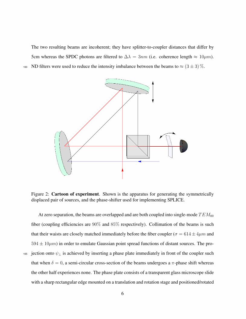
ND filters were used to reduce the intensity imbalance between the beams to ≈ (3± 3) %.100

Figure 2: Cartoon of experiment. Shown is the apparatus for generating the symmetricallydisplaced pair of sources, and the phase-shifter used for implementing SPLICE.

At zero separation, the beams are overlapped and are both coupled into single-mode TEM00

fiber (coupling efficiencies are 90% and 85% respectively). Collimation of the beams is such

that their waists are closely matched immediately before the fiber coupler (σ = 614± 4µm and

594 ± 10µm) in order to emulate Gaussian point spread functions of distant sources. The pro-

jection onto ψ⊥ is achieved by inserting a phase plate immediately in front of the coupler such105

that when δ = 0, a semi-circular cross-section of the beams undergoes a π-phase shift whereas

the other half experiences none. The phase plate consists of a transparent glass microscope slide

with a sharp rectangular edge mounted on a translation and rotation stage and positioned/rotated

6

to minimize coupling into an otherwise well-aligned coupler. Typical visibility is ≥ 99%.

To compare the performance of our method with a more traditional imaging setup, we re-110

placed the phase plate with a 200µm slit that served as the image plane, coupling all the light

transmitted through the slit into a multimode fibre. Scanning the slit, we were able to perform

one-dimensional IPC.

With SPLICE, the separation of the incoherent beams was scanned, with the detectors count-

ing for 1 second at each step. Two sets of these “phase-plate” scans were performed, one at115

coarse intervals of δ (spanning−1.96mm to +1.94mm, in steps of 0.1mm) and another at finer

intervals (−0.56mm ≤ δ ≤ +0.44mm in steps of 0.04mm). Data from nine repetitions of the

coarse scan and fifteen of the fine scan were recorded.

Figure 3: Inferred separation vs known actual separation for a) SPLICE (from “lookup” oncalibration curve) and b) IPC.

Whereas the ideal functional form for the resulting counts vs separation δ is proportional to

7

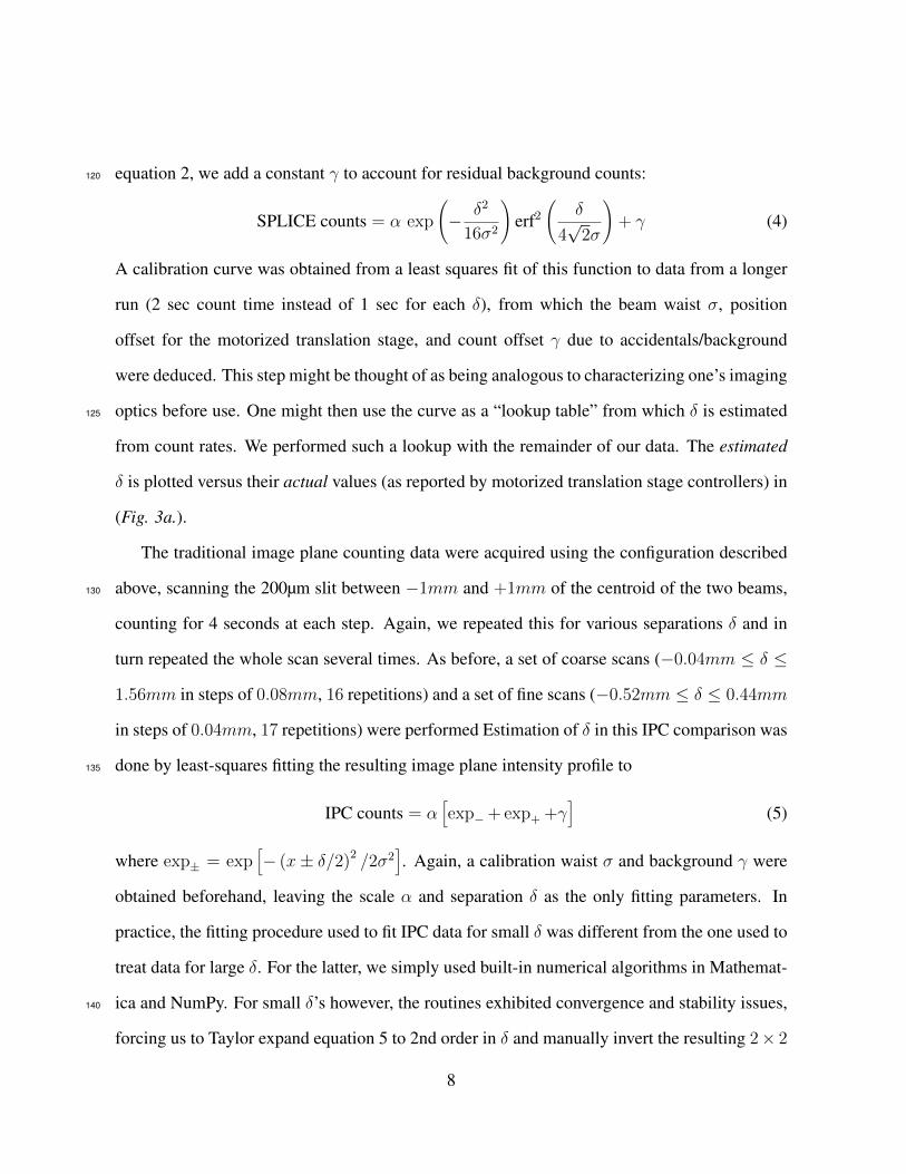
equation 2, we add a constant γ to account for residual background counts:120

SPLICE counts = α exp

(− δ2

16σ2

)erf2

(δ

4√

2σ

)+ γ (4)

A calibration curve was obtained from a least squares fit of this function to data from a longer

run (2 sec count time instead of 1 sec for each δ), from which the beam waist σ, position

offset for the motorized translation stage, and count offset γ due to accidentals/background

were deduced. This step might be thought of as being analogous to characterizing one’s imaging

optics before use. One might then use the curve as a “lookup table” from which δ is estimated125

from count rates. We performed such a lookup with the remainder of our data. The estimated

δ is plotted versus their actual values (as reported by motorized translation stage controllers) in

(Fig. 3a.).

The traditional image plane counting data were acquired using the configuration described

above, scanning the 200µm slit between −1mm and +1mm of the centroid of the two beams,130

counting for 4 seconds at each step. Again, we repeated this for various separations δ and in

turn repeated the whole scan several times. As before, a set of coarse scans (−0.04mm ≤ δ ≤

1.56mm in steps of 0.08mm, 16 repetitions) and a set of fine scans (−0.52mm ≤ δ ≤ 0.44mm

in steps of 0.04mm, 17 repetitions) were performed Estimation of δ in this IPC comparison was

done by least-squares fitting the resulting image plane intensity profile to135

IPC counts = α[exp−+ exp+ +γ

](5)

where exp± = exp[− (x± δ/2)2 /2σ2

]. Again, a calibration waist σ and background γ were

obtained beforehand, leaving the scale α and separation δ as the only fitting parameters. In

practice, the fitting procedure used to fit IPC data for small δ was different from the one used to

treat data for large δ. For the latter, we simply used built-in numerical algorithms in Mathemat-

ica and NumPy. For small δ’s however, the routines exhibited convergence and stability issues,140

forcing us to Taylor expand equation 5 to 2nd order in δ and manually invert the resulting 2× 2

8

design matrix. The resulting estimated separations are plotted against actual separations in (Fig.

3b.). As is immediately apparent, for separations below about 0.25mm (approximately 0.4σ),

the spread of the IPC data begins to grow, while that of the SPLICE data remains essentially

constant.145

Two key metrics for the performance of either method are the standard deviation or SD

(i.e. “spread”) and root-mean-square error (RMSE) of the estimated beam separation. The SD

measures the precision of a dataset but not necessarily its accuracy, while the RMSE is sensitive

to the accuracy since it quantifies the error relative to a known actual value and not simply

the reported result. In (Fig. 4. and Fig. 5.), SD and RMSE are plotted versus known actual150

separations.

Figure 4: Uncertainty comparison between SPLICE and IPC. Standard Deviation (SD) inthe estimated separation plotted as a function of actual separation for both IPC and SPLICE.The computed SD for each dataset is multiplied by photon number (

√N ). Overlayed lines are

the corresponding Monte Carlo simulations. Note that two methods were used in the fittingof IPC data to equation 5; for small δ (< 0.65mm), equation 5 was expanded to 2nd order andlinear regression was performed whereas for large δ (> 0.4mm), a nonlinear fitting routine builtinto Mathematica was used.

9

Figure 5: Un-normalized Root Mean-Square Error (RMSE) in the estimated separation vsactual separation for both IPC and SPLICE. Unlike SD, the RMSE allows us to gauge absoluteerror relative to the known actual value of the parameter being estimated so that biases areaccounted for. Note that two methods were used in the fitting of IPC data to equation 5; for smallδ (< 0.65mm), equation 5 was expanded to 2nd order and linear regression was performedwhereas for large δ (> 0.4mm), a nonlinear fitting routine built into Mathematica was used.

In order to ensure a reasonably even-footed comparison between IPC and SPLICE, the

spreads in inferred separation plotted in (Fig. 4.) are scaled by√N (where N is the pho-

ton number that comprises a measurement) to reflect the fact that noise in photon counts at our

detector is Poissonian. For IPC, N is simply the total photons that comprise an “image” on the155

image plane, which in our case is actually a set of photon counts, one at each position of the

200µm slit. For SPLICE, during a calibration run, we estimate N by counting at our detector

over a 1 second window while both beams are centered (i.e. δ = 0) on the coupler into TEM00

fiber with the phase-plate removed. Since our source intensity is stable, this gives us an estimate

of the number of incident photons for subsequent measurements when δ 6= 0.160

The RMSE plotted in (Fig. 5.) is not similarly normalized because in addition to possible

10

systematics, the inferred separation is biased relative to the actual separation when δ is small.

A priori, there is no reason to suspect either bias or systematics to scale as√N . Despite not

normalizing and despite using approximately twice as many photons, the IPC method performs

noticeably worse than SPLICE when δ < 0.6mm.165

The attentive reader will note that while the spread is greater for IPC, it does not diverge as

δ → 0. In fact, it would be implausible for the uncertainty on δ to ever exceed σ. The apparent

discrepancy with the vanishing of the Fisher information can be understood by recognizing that

(as is clear from inspection of (Fig. 1.) at small δ) the practically implemented IPC estimator is

not unbiased. To better understand the bounds on the advantage that one can expect of SPLICE170

over IPC, we return to equation 1. Clearly, one needs to know the bias to evaluate the RHS.

For SPLICE, the only potential source of bias is the lookup procedure. If, for example, a

less-than-perfect visibility results in a calibration curve that does not vanish at δ = 0, then

one might obtain “unphysical” datapoints that fall under the minima of the calibration curve,

thereby resulting in a bias when a lookup is attempted. In our case, this is negligible since175

our visibility exceeds 99%. The CRLB is therefore just the reciprocal of If , implying a 1/√N

scaling in the spread of δest.

With IPC, the least-squares estimate of δ is heavily biased at small δ. An intuitive way to

understand this is to note that since the problem being addressed is the resolving of two equal

intensity sources, the +δ and −δ cases are physically indistinguishable. This is equivalent to180

saying that the power series expansion of equation 5 consists only of even powers of δ. Given no

additional information about the sign of δ, we restrict δ to be positive without loss of generality.

But in doing so, as long as spread in the estimated δ is non-zero, the mean estimated δ is never

zero. (Fig. 6.) shows a plot of mean inferred δ (averaged across all our datasets) vs actual δ.

Overlayed is a theory curve for IPC, which takes into account an expected bias at small δ.185

In [23], we present theory showing that the bias term for IPC falls to−1 sufficiently quickly

11

that the RHS of inequality 1 tends to a finite value as δ → 0. That finite value is shown to

scale as N−1/4, which is in stark contrast to the behaviour of the spread at large δ (for IPC)

as well as for SPLICE (at all δ), where a Poissonian scaling of N−1/2 is obeyed. This scaling

is further substantiated with Monte-Carlo simulations shown in a figure in [23]. Thus while190

SPLICE does not offer an infinite advantage over IPC as a naive analysis might have us believe,

it does nevertheless offer a substantial improvement in the absolute error and the scaling with

photon number, while simultaneously eliminating the problem of bias.

12

Figure 6: Averaged measured separations. Mean estimated δ for IPC and SPLICE plottedagainst known actual δ. Two methods were used in the fitting of IPC data to equation 5; for smallδ (< 0.65mm), equation 5 was expanded to 2nd order and linear regression was performedwhereas for large δ (> 0.4mm), a nonlinear fitting routine built into Mathematica was used.

In summary, we have developed and demonstrated a simple technique that surpasses tradi-

tional imaging in its ability to resolve two closely spaced point-sources. Furthermore, unlike195

existing superresolution methods, ours requires no exotic illumination with particular coher-

ence/quantum properties and is applicable to classical incoherent sources. Crucially, as a proof-

of-principle, this technique highlights the importance of realising that diffraction-imposed reso-

lution limits are not a fundamental constraint but, instead, the consequence of traditional imag-

13

ing techniques discarding the phase information present in the light. We expect that this and200

other related techniques that do not discard the phase information will be developed in the future

for a broad range of imaging applications.

Note: While preparing this manuscript, we came to realise that similar work was being

pursued by Yang et al [24] and Sheng et al [25].

References and Notes205

[1] Lord Rayleigh. XXXI. Investigations in optics, with special reference to the spectroscope.

Philosophical Magazine Series 5 8, 261–274 (1879). URL http://dx.doi.org/

10.1080/14786447908639684.

[2] Hell, S. W. & Wichmann, J. Breaking the diffraction resolution limit by stimulated emis-

sion: stimulated-emission-depletion fluorescence microscopy. Optics letters 19, 780–782210

(1994).

[3] Betzig, E. et al. Imaging intracellular fluorescent proteins at nanometer resolution. Science

313, 1642–1645 (2006).

[4] Hess, S. T., Girirajan, T. P. & Mason, M. D. Ultra-high resolution imaging by fluorescence

photoactivation localization microscopy. Biophysical journal 91, 4258–4272 (2006).215

[5] Giovannetti, V., Lloyd, S. & Maccone, L. Quantum-enhanced measurements: beating the

standard quantum limit. Science 306, 1330–1336 (2004).

[6] Giovannetti, V., Lloyd, S. & Maccone, L. Advances in quantum metrology. Nature Pho-

tonics 5, 222–229 (2011).

[7] Mitchell, M. W., Lundeen, J. S. & Steinberg, A. M. Super-resolving phase measurements220

with a multiphoton entangled state. Nature 429, 161–164 (2004).

14

[8] Walther, P. et al. De broglie wavelength of a non-local four-photon state. Nature 429,

158–161 (2004).

[9] Nagata, T., Okamoto, R., O’Brien, J. L., Sasaki, K. & Takeuchi, S. Beating the standard

quantum limit with four-entangled photons. Science 316, 726–729 (2007).225

[10] Tsang, M., Nair, R. & Lu, X. Quantum theory of superresolution for two incoherent

optical point sources. arXiv preprint arXiv:1511.00552 (2015).

[11] Casella, G. & Berger, R. L. Statistical inference, vol. 2 (Duxbury Pacific Grove, CA,

2002).

[12] Helstrom, C. W. Quantum detection and estimation theory. Journal of Statistical Physics230

1, 231–252 (1969).

[13] Petz, D. & Ghinea, C. Introduction to quantum fisher information. Quantum Probability

and Related Topics 1, 261–281 (2011).

[14] Hemmer, P. R. & Zapata, T. The universal scaling laws that determine the achievable

resolution in different schemes for super-resolution imaging. Journal of Optics 14, 083002235

(2012).

[15] Giovannetti, V., Lloyd, S., Maccone, L. & Shapiro, J. H. Sub-rayleigh-diffraction-bound

quantum imaging. Physical Review A 79, 013827 (2009).

[16] Tsang, M. Quantum imaging beyond the diffraction limit by optical centroid measure-

ments. Physical review letters 102, 253601 (2009).240

[17] Shin, H., Chan, K. W. C., Chang, H. J. & Boyd, R. W. Quantum spatial superresolution

by optical centroid measurements. Phys. Rev. Lett. 107, 083603 (2011).

15

[18] Rozema, L. A. et al. Scalable spatial superresolution using entangled photons. Phys. Rev.

Lett. 112, 223602 (2014).

[19] Tamburini, F., Anzolin, G., Umbriaco, G., Bianchini, A. & Barbieri, C. Overcoming the245

rayleigh criterion limit with optical vortices. Phys. Rev. Lett. 97, 163903 (2006).

[20] Schwartz, O. et al. Superresolution microscopy with quantum emitters. Nano letters 13,

5832–5836 (2013).

[21] Richardson, D., Fini, J. & Nelson, L. Space-division multiplexing in optical fibres. Nature

Photonics 7, 354–362 (2013).250

[22] For circular apertures, the point spread functions are Airy rings. In practice, these are

often well-approximated by Gaussians. Within this approximation, two overlapped point-

sources map simply to a single Gaussian.

[23] Supplementary material and extended data are available online.

[24] Yang, F., Taschilina, A., Moiseev, E. S., Simon, C. & Lvovsky, A. I. Far-field linear255

optical superresolution via heterodyne detection in a higher-order local oscillator mode.

ArXiv e-prints (2016). 1606.02662.

[25] Sheng, T. Z., Durak, K. & Ling, A. Fault-tolerant and finite-error localization for point

emitters within the diffraction limit. arXiv preprint arXiv:1605.07297 (2016).

Acknowledgment260

This work was funded by NSERC, CIFAR, and Northrop-Grumman Aerospace Systems. We

would like to thank Mankei Tsang for useful discussions and the Facebook post which led to

this collaboration.

16

Author Contribution

W.K.T. and H.F. jointly conducted theoretical analysis, designed and performed the experi-265

ment, and analyzed data. A.M.S. conceived of the SPLICE scheme, guided its experimental

implementation, and oversaw the research project. All authors contributed to the writing of this

article.

Competing Interest

We declare no competing financial interests.270

Correspondence

Correspondence and material requests should be adressed to H. F. (hferrett@physics.utoronto.ca).

17

Extended Data

Figure 7: Raw data plot for SPLICE coarse scans. Dots are experimental photon coin-cidence counts plotted versus actual beam seperation δ. Solid overlay is a fit to equation2.

18

Figure 8: Monte-Carlo Scaling Analysis. Dots are the SD in inferred separation from Monte-Carlo simulations of SPLICE (blue) and IPC (red), with δ = 0.21mm averaged over 200 rep-etitions versus total photon number. Other parameters - i.e. σ and γ/N (see text) - were set toexperimental values. The overlayed solid lines power-law fits of the form αNβ to simulationresults. The fit parameters for IPC are: α = 0.943 ± 0.031, β = −0.254 ± 0.004 and forSPLICE α = 2.188± 0.090, β = −0.521± 0.006. While δ = 0.21mm was chosen arbitrarilyfor this plot, the simulation was performed for multiple values of δ. We note that with finitevisibility (i.e. γ 6= 0), SPLICE also begins to scale as N−1/4 when both δ and N are very small.It is important to note, however, that unlike IPC, this is not a fundamental scaling but is rather aresult of technical limitations (i.e. imperfect visibility) in our apparatus. A scaling of N−1/2 isretained for all δ and N when γ = 0.

275

19

Supplementary

Bias Derivation

Bias

Suppose one was tasked with estimating the value of some parameter, x, by looking at the

value of some random variable y, which distribution depends on x. If the expectation value of280

y equals x for all values of the parameter x, i.e. 〈y〉x = x, then the random variable y is known

as an unbiased estimator of x. The distinction between a biased vs an unbiased estimator

is important to consider when one is trying to reason in terms of the Fisher information and

CRLB. As mentioned in the main text, a more general form of the CRLB is:

√Var (y) ≥

√√√√ 1

Ifish

(1 +

∂ (bias)∂x

)

where bias is 〈y〉x − x. Notice that when the estimator is unbiased, this reduces to equation 4285

in the main text. In the case of IPC, since the Fisher information clearly vanishes as δ → 0, an

infinite variance in the estimator δest can be avoided only if the slope of 〈y〉x tends to 0 more

quickly than Ifish. It is our goal in this supplementary section to demonstrate that that is indeed

the case.

Spread in estimator of δ2290

For IPC at small separations each image was fitted to a Taylor expansion of the detection

probability pi (the usual sum of two Gaussians) to 2nd order:

pi ≈A

σ√

2πexp

[− x2

i

2σ2

]+

Aδ2

8σ5√

2πexp

[− x2

i

2σ2

] (x2i − σ2

)Subscripts i were added in anticipation of an image consisting of many pixels at various values

of some axis x. Performing a linear regression of a set of photon detection rates pi yields

parameters A and Aδ2. Notice that the design matrix, M , in this case contains only xi’s and295

σ and so is independent of photon number N . If we now assume that the noise at each pixel

20

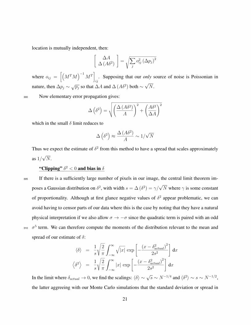
location is mutually independent, then:[∆A

∆ (Aδ2)

]=√∑

j

o2ij (∆pj)

2

where oij =[(MTM

)−1MT

]ij

. Supposing that our only source of noise is Poissonian in

nature, then ∆pj ∼√pj so that ∆A and ∆ (Aδ2) both ∼

√N .

Now elementary error propagation gives:300

∆(δ2)

=

√√√√(∆ (Aδ2)

A

)2

+

(Aδ2

∆A

)2

which in the small δ limit reduces to

∆(δ2)≈ ∆ (Aδ2)

A∼ 1/

√N

Thus we expect the estimate of δ2 from this method to have a spread that scales approximately

as 1/√N .

“Clipping” δ2 < 0 and bias in δ

If there is a sufficiently large number of pixels in our image, the central limit theorem im-305

poses a Gaussian distribution on δ2, with width s = ∆ (δ2) = γ/√N where γ is some constant

of proportionality. Although at first glance negative values of δ2 appear problematic, we can

avoid having to censor parts of our data where this is the case by noting that they have a natural

physical interpretation if we also allow σ → −σ since the quadratic term is paired with an odd

σ5 term. We can therefore compute the moments of the distribution relevant to the mean and310

spread of our estimate of δ:

〈δ〉 =1

s

√2

π

ˆ ∞−∞

√|x| exp

[−(x− δ2

actual)2

2s2

]dx

⟨δ2⟩

=1

s

√2

π

ˆ ∞−∞|x| exp

[−(x− δ2

actual)2

2s2

]dx

In the limit where δactual → 0, we find the scalings: 〈δ〉 ∼√s ∼ N−1/4 and 〈δ2〉 ∼ s ∼ N−1/2,

the latter aggreeing with our Monte Carlo simulations that the standard deviation or spread in

21

our estimate scales as N−1/4 as well. More crucially, 〈δ〉 can be shown to approach a constant

value sufficiently quickly as δactual goes to 0 for the CRLB to converge to a finite value. 〈δ〉 is315

plotted in figure 8 of the main text.

Note that the emergence of a bias in our estimate isn’t specific to our treatment of the

negative tail of δ2; the same bias and scalings can be obtained even if we had opted for the

lazier approach of censoring parts of our data that produce negative δ2 values (tantamount to

simply “chopping” rather than “folding” that tail of the distribution). Rather, the bias is more320

generally a consequence of performing the regression on δ2 instead of δ.

The bias vanishes if the two sources have unequal intensities. The breaking of this symmetry

introduces a term in pi that is linear in δ. If this term is much larger than the quadratic (δ2) term,

we can use δ as a fit parameter instead, thereby obtaining an unbiased estimator. We leave the

analysis of this asymmetric case to a possible future work.325

22