
Bearing Capacity Of Shallow Foundation -...
46
Bearing Capacity Of Shallow Foundation
-
Upload
duongtuyen -
Category
Documents
-
view
227 -
download
2
Transcript of Bearing Capacity Of Shallow Foundation -...

Bearing Capacity Of Shallow
Foundation

Bearing Capacity Of Shallow Foundation * A foundation is required for distributing
the loads of the superstructure on a large area. * The foundation should be designed such that a) The soil below does not fail in shear & b) Settlement is within the safe limits.
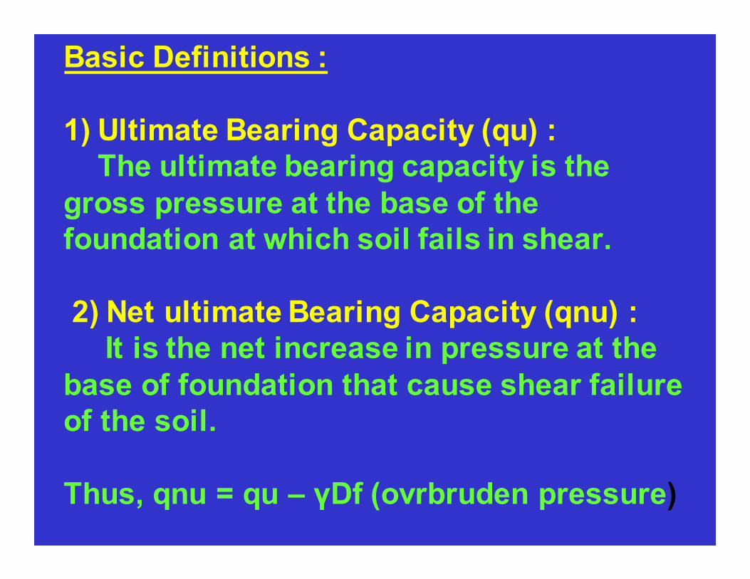
Basic Definitions :
1) Ultimate Bearing Capacity (qu) : The ultimate bearing capacity is the
gross pressure at the base of the foundation at which soil fails in shear.
2) Net ultimate Bearing Capacity (qnu) : It is the net increase in pressure at the
base of foundation that cause shear failure of the soil.
Thus, qnu = qu – γDf (ovrbruden pressure)

3) Net Safe Bearing Capacity (qns) :
It is the net soil pressure which can be
safely applied to the soil considering only shear
failure.
Thus, qns = qnu /FOS
FOS - Factor of safety usually taken as 2.00 -3.00
4) Gross Safe Bearing Capacity (qs) :
It is the maximum pressure which the soil can
carry safely without shear failure.
qs = qnu / FOS + γ Df
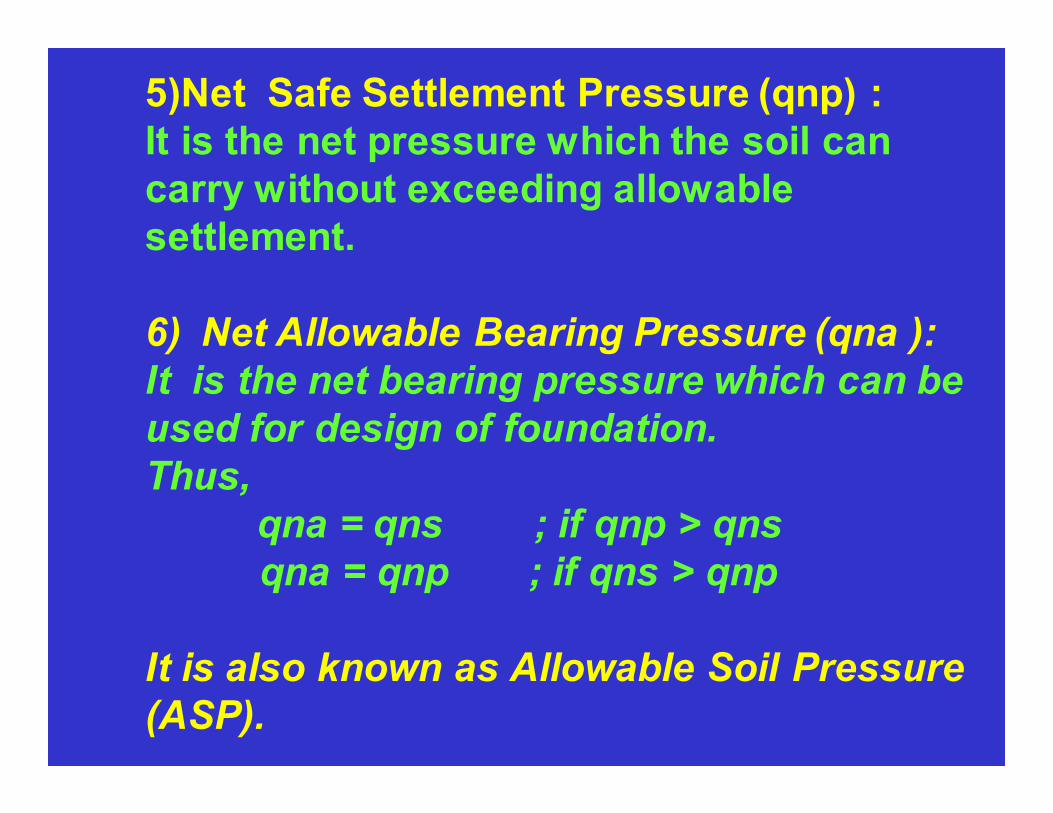
5)Net Safe Settlement Pressure (qnp) : It is the net pressure which the soil can carry without exceeding allowable settlement.
6) Net Allowable Bearing Pressure (qna ):
It is the net bearing pressure which can be
used for design of foundation.
Thus,
qna = qns ; if qnp > qns
qna = qnp ; if qns > qnp
It is also known as Allowable Soil Pressure
(ASP).
Modes of shear Failure : Vesic (1973) classified shear failure of soil under a foundation base into three categories depending on the type of
soil & location of foundation. 1) General Shear failure.
2) Local Shear failure. 3) Punching Shear failure

General Shear failure –
Strip footing resting on surface Load –settlement curve
of dense sand or stiff clay
* The load - Settlement curve in case of footing resting on surface of dense sand
or stiff clays shows pronounced peak & failure occurs at very small stain.
* A loaded base on such soils sinks or tilts suddenly in to the ground showing a
surface heave of adjoining soil
* The shearing strength is fully mobilized all along the slip surface & hence
failure planes are well defined.
* The failure occurs at very small vertical strains accompanied by large lateral
strains.
* ID > 65 ,N>35, Φ > 360, e < 0.55

2) Local Shear failure -
* When load is equal to a certain value qu(1),
* The foundation movement is accompanied by sudden jerks.
* The failure surface gradually extend out wards from the foundation.
* The failure starts at localized spot beneath the foundation & migrates out
ward part by part gradually leading to ultimate failure.
* The shear strength of soil is not fully mobilized along planes & hence
failure planes are not defined clearly.
* The failure occurs at large vertical strain & very small lateral strains.
* ID = 15 to 65 , N=10 to 30 , Φ <30, e>0.75
Strip footing resting on surface Load –settlement curve
Of Medium sand or Medium clay
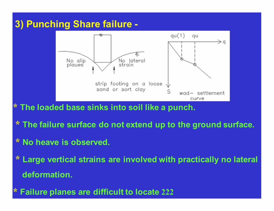
3) Punching Share failure -
* The loaded base sinks into soil like a punch.
* The failure surface do not extend up to the ground surface.
* No heave is observed.
* Large vertical strains are involved with practically no lateral
deformation.
* Failure planes are difficult to locate 222

Terzaghi’s Bearing Capacity Analysis –
Terzaghi (1943) analysed a shallow continuous footing by
making some assumptions –

* The failure zones do not extend above the
horizontal plane passing through base of footing
* The failure occurs when the down ward pressure
exerted by loads on the soil adjoining the inclined surfaces on soil wedge is equal to upward
pressure.
* Downward forces are due to the load (=qu× B) &
the weight of soil wedge (1/4 γB2 tanØ)
* Upward forces are the vertical components of
resultant passive pressure (Pp) & the cohesion (c’) acting along the inclined surfaces.
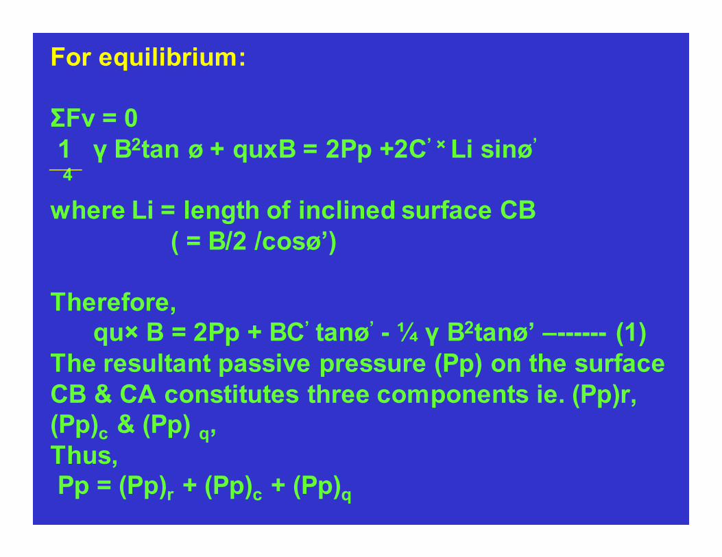
For equilibrium:
ΣFv = 0
1 γ B2tan ø + quxB = 2Pp +2C’ × Li sinø’
4
where Li = length of inclined surface CB
( = B/2 /cosø’)
Therefore, qu× B = 2Pp + BC’ tanø’ - ¼ γ B2tanø’ –------ (1)
The resultant passive pressure (Pp) on the surface
CB & CA constitutes three components ie. (Pp)r, (Pp)c & (Pp) q,
Thus, Pp = (Pp)r + (Pp)c + (Pp)q

qu× B= 2[ (Pp)r +(Pp)c +(Pp)q ]+ Bc’tanø’-¼ γ B2 tanø’
Substituting; 2 (Pp)r - ¼rB2tanø1 = B × ½ γ BNr
2 (Pp)q = B × γ D Nq
& 2 (Pp)c + Bc1 tanø1 = B × C1 Nc;
We get,
qu =C’Nc + γ Df Nq + 0.5 γ B N γ
This is Terzaghi’s Bearing capacity equation for
determining ultimate bearing capacity of strip footing.
Where Nc, Nq & Nr are Terzaghi’s bearing capacity
factors & depends on angle of shearing resistance (ø)

ø General Shear Failure Local Shear Failure
Nc Nq Nr Nc’ Nq’ Nr’
0 5.7 1.0 0.0 5.7 1.0 0.0
15 12.9 4.4 2.5 9.7 2.7 0.9
45 172.3 173.3 297.5 51.2 35.1 37.7

Important points :
* Terzaghi’s Bearing Capacity equation is applicable
for general shear failure.
* Terzaghi has suggested following empirical reduction to
actual c & ø in case of local shear failure
Mobilised cohesion Cm = 2/3 C
Mobilised angle of øm = tan –1 (⅔tanø)
Thus, Nc’,Nq’ & Nr’ are B.C. factors for local shear failure
qu = CmNc’+ γ Df Nq’+ 0.5 γ B Nr’
* Ultimate Bearing Capacity for square & Circular footing -Based
on the experimental results, Terzaghi’s suggested following
equations for UBC –
Square footing qu = 1.2c’ Nc + γ Df Nq + 0.4 γ BNr
Circular footing qu = 1.2c1Nc + γ Df Nq + 0.3 γ BNr

Effect of water table on Bearing Capacity : * The equation for ultimate bearing
capacity by Terzaghi has been developed based on assumption that water table is located at a great depth . * If the water table is located close to foundation ; the equation needs modification.

i) When water table is located above the base of
footing -
* The effective surcharge is reduced as the
effective weight below water table is equal to submerged unit weight.
q = Dw.r +x.γsub put x = Df-Dw
q = γsub Df +( γ- γsub)Dw
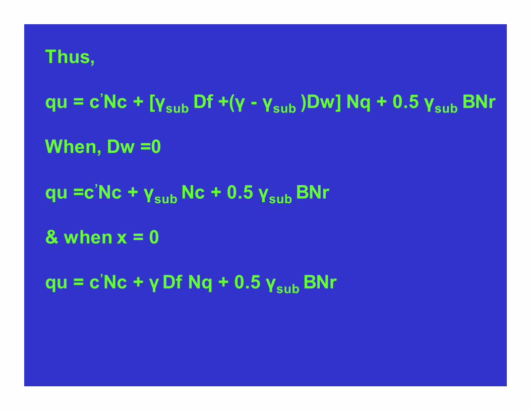
Thus,
qu = c’Nc + [γsub Df +(γ - γsub )Dw] Nq + 0.5 γsub BNr
When, Dw =0
qu =c’Nc + γsub Nc + 0.5 γsub BNr
& when x = 0
qu = c’Nc + γ Df Nq + 0.5 γsub BNr
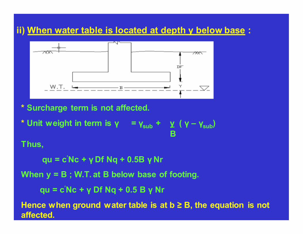
ii) When water table is located at depth y below base :
* Surcharge term is not affected.
* Unit weight in term is γ = γsub + y ( γ – γsub)
B Thus,
qu = c’Nc + γ Df Nq + 0.5B γ Nr
When y = B ; W.T. at B below base of footing.
qu = c’Nc + γ Df Nq + 0.5 B γ Nr
Hence when ground water table is at b ≥ B, the equation is not affected.

Hansen’s Bearing Capacity Equation :
Hansen’s Bearing capacity equation is :
qu = cNcScdcic + qNqSqdqiq + 0.5 γ BNrSrdr ir
where,
Nc,Nq, & Nr are Hansen’s B.C factors which are some what smaller than Terzaghi’s B.C. factors. Sc.Sq &Sr are shape factors which are independent of angle of shearing resistance; dc,dq, & dr are depth factors ;
Ic, iq & ir are iodination factors

The same form of equation has been
adopted by I.S. 6403 –1971 & may be used for general form as
qnu = c Nc Sc dc ic + q(Nq-1)Sqdqiq + 0.5 γ BNrSrdr ir W’

Settlement of foundation :
a) Settlement under loads
Settlement of foundation can be classified as-
1. Elastic settlement (Si): Elastic or immediate
settlement takes place during or immediately after the construction of the structure. It is also known as
the distortion settlement as it is due to distortions
within foundation soil.
2. Consolidation settlement (Sc): Consolidation
settlement occurs due to gradual expulsion of water
from the voids at the soil. It is determined using
Terzaghi's theory of consolidation.
3. Secondary consolidation settlement (Ss): The
settlement occurs after completion of the primary
consolidation. The secondary consolidation is non-
significant for inorganic soils.

Thus,
Total settlement (s) = Si+ Sc + Ss
b) Settlement due to other causes
1. Structural collapse of soil. 2. Underground erosion.
3. Lowering of water table. . 4. Thermal changes.
5. Subsidence etc.

Elastic settlement of foundation :
a) On Cohesive soils
According to schleicher, the vertical settlement
under uniformly distributed flexible area is,
Si = q B 1- µ2/Es I
where q -uniformly distributed load.
B - characteristic length of loaded area,
Es - modulus of elasticity of the soil.
µ - poisson's ratio.
I - influence factor which dependent upon elastic properties of base & shape at base.
Alternatively, the value of [1- µ2/Es] I can be
determined from the plate load test.

b) On Cohesionless Soils According to Stuartmann & Hartman immediate
settlement on Cohesionless soils is given by -
Where, C1 -Correction factor for depth of foundation
embedment
C2 - correction factor for creep is soils. q - pressure at the level of foundation
q -surcharge (γ Df)
Es- modulus of elasticity = 766 N (KN/m2) from SPT
= 2qc from SCPT
( ) ∫=
∈∆−=ZB
Z S
iE
IqqCCS
0
221

Settlement of foundation on Cohesionless Soils
Settlement of foundations on Cohesionless soils are generally determined indirectly using the semi-empirical
methods. 1. Static Cone Penetration method
In this, the sand layer is divided into small layers such that each small layer has approximately constant value
of the cone resistance. The average value of the cone resistance of each small layer is determined.
The settlement of each layer is determined using the following equation-
S = H/C Log (σ0 + ∆ σ) / σ0
Where, c = 1.5 qc/ σ0

in which qC - static cone resistance
σ0 - mean effective overburden pressure,
∆ σ - Increase is pressure at center of layer due to net foundation pressure.
H - thickness of layer. The total settlement of the entire layer is equal to the sum of settlements of individual layers.
2. Standard Penetration Test
IS 8009 (part I) 1976 gives a chart for the calculation of settlement per unit pressure as a foundation of the width of footing & the standard penetration number.
3. Plate Load Test
The settlement of the footing can be determined from the settlement of the plate in the plate load test.

Differential Settlement :
* The difference between the magnitudes of
settlements at any two points is known as
differential settlement.
* If there is large differential settlement
between various part of a structure, distortion
may occur due to additional moments
developed.
* The differential settlement may caused due
to tilting of a rigid base, dishing of flexible
base or due to non uniformity of loading.
* If S1 & S2 are the settlements at two
points,then differential settlement is
∆∆∆∆ = S1 -S2
Angular distortion = (S1- S2 ) / L = ∆∆∆∆ /L

* It is difficult to predict the differential
settlement. * It is generally observed indirectly from the maximum settlement.
* It is observed that the differential settlement is less than 50% of the
maximum settlement is most of the cases. The differential settlement can be
reduced by providing rigid rafts, founding the structures at great depth
& avoiding the eccentric loading.

Allowable Settlement
* The allowable maximum settlement depends upon the type of soil, the type of
foundation & the structural framing system.
* The maximum settlement ranging from
20mm to 300mm is generally permitted for various structures.
* IS 1904-1978 gives values of the maximum
& differential settlements of different type of
building.

Sand & hard
Clay
Plastic clay
Max.Settle. Diff.Settl Angular
distortion
Max.Settle Diff. Settle.
Angular
distortion
Isolated foundation
i) steel struct ii) RCC struct
50mm
50mm
0.0033L
0.0015L
1/300
1/666
50mm
75mm
0.0033L
0.0015L
1/300
1/666
Raft foundation
i) steel struct ii) Rcc struct.
75mm
75mm
0.0033L
0.002L
1/300
1/500
100mm
100mm
0.0033L
0.002L
1/300
1/500
Theoretically, no damage is done to the superstructure
if the soil settles uniformly.
However, settlements exceeding 150mm may cause
trouble to utilities such as water pipe lines, sewers,
telephone lines & also is access from streets.

Consolidation Settlement :
* Compressibility of soil is the property of the soil due to
which a decrease in volume occurs under compressive
forces.
* The compression of soils can occurs due to-
A) Compression of solid particles & water in the voids. B) Compression & expulsion of air in the voids.
C) Expulsion of water in the voids.
* The compression of a saturated soil under a steady
pressure is known as consolidation. It is entirely due to
expulsion of water from the voids. Due to expulsion of
water, the solid particle shift from one position to the other by rolling & sliding & thus attain a closer packing causing
reduction in volume.

Consolidation of laterally confined soil:
When a pressure ∆∆∆∆ σσσσ, is applied to a saturated soil
sample of unit cross- sectional area, the pressure is
shared by the solid particles & water as
∆∆∆∆ σσσσ + u = ∆∆∆∆ σσσσ,
Initially, just after the application of pressure, the
entire load is taken by water in form of excess
hydrostatic pressure ( u ), thus,
0 + ( u , ) = ∆∆∆∆ σσσσ, The excess hydrostatic pressure so developed sets
up a hydraulic gradient, & the water starts escaping
from the voids. As the water escapes, the applied
pressure is transferred from the water to the solids.
Thus at t = tf, ∆∆∆∆ σσσσ + 0 = ∆∆∆∆ σσσσ,
As the effective stress increases the volume of soil
decreases & consolidation completes under ∆∆∆∆ σσσσ, load.

Laboratory Consolidation Test:
* The consolidation test is conducted in a laboratory study
the compressibility of soil.
* Consolidation test apparatus, known as consolidometer or
an odometer consists a loading device & a cylindrical
container called as consolidation cell. Consolidation cell are of
two types, i) free ring or floating ring cell &
ii) fixed ring cell
* The internal diameter of the cell is 60 mm & thickness of
sample taken is usually 20 mm.
* The consolidometer has arrangements for application of
the desired load increment,saturation of sample &
measurement of change in thickness of sample at every stage
of consolidation process
* An initial setting load of about 5 kN/ m 2 is applied to sample.
* The first increment of load to give a pressure of 10 KN/ m2 is then
applied to the specimen, the dial gauge readings are taken after 0.25,
1.0, 2,4,9,16,…… etc up to the 24 hours.
* The second increment of load is then applied. The successive
pressures usually applied are 20,40, 80, 160 & 320 KN/ m 2 etc till the
desired maximum load intensity is reached.
( Actual loading on soil after construction of structure)
* After consolidation under final load increment is complete, the load
is reduced to ¼th of final load & allowed to stand for 24 hours. The
sample swells & reading of dial gauge is taken when swelling is
complete. The process is repeated till complete unloading.
Immediately after complete unloading, the weight of ring & sample is
taken. The sample is dried in over for 24 hours & its dry mass Ms is
taken.

Consolidation test results
1) Dial gauge reading time plot :
•••• Plotted for each load increment •••• Required for determining the coefficient of consolidation.
•••• Useful for obtaining the rate of consolidation in field.

2) Final void ratio – effective stress plot:
•••• Plotted for entire consolidation process under
desired load.
•••• Required for determination of the magnitude of the
consolidation settlements in field.

3) final void ratio – log σσσσ plot

4)Loading, unloading & reloading plot

Important Definations
1) Coefficient of compressibility ( av) is defined as
decrease in void ratio per unit increase in effective stress.
av = -de/dσσσσ = -∆∆∆∆e/ ∆σ∆σ∆σ∆σ ( slope of e - σσσσ curve units – m 2 /KN ) 2) Coefficient of volume change ( mv) is defined as the
volumetric strain per unit increase in effective stress.
mv = - (∆∆∆∆v / v o)/ ∆σ∆σ∆σ∆σ in which,
vo – initial volume,
∆∆∆∆v – change in volume
∆∆∆∆ σσσσ - change in effective stress
a) mv = -(∆∆∆∆e / 1+ eo)/ ∆∆∆∆ σσσσ
b) for one dimension, ∆∆∆∆v = ∆∆∆∆H
mv = - (∆∆∆∆H / Ho) / ∆σ∆σ∆σ∆σ
also mv = av / (1+ eo ) in which, eo- initial void ratio.
∆∆∆∆e - change in void ratio.
Ho initial thickness.
∆∆∆∆H – change in thickness.

3) Compression index ( Cc) is equal to the slope
of the linear portion of the void ration versus log σσσσ plot.
Cc = - ∆∆∆∆ e/ log 10 (σσσσ 0 + ∆∆∆∆ σσσσ) / σσσσ0
in which, σσσσ0 = initial effective stress. ∆σ∆σ∆σ∆σ - change in effective stress.
Empirical relationship after Terzaghi & Peck;
a) for undisturbed soils Cc = 0.009 ( W L- 10 )
b) for remoulded soils Cc = 0.007 ( W L- 10 ) c) Also Cc = 0.54 ( eo – 0.35 )
Cc = 0.0054 ( 2.6 wo- 35 )

•••• Normally consolidated soil :- A normally
consolidated soil is one which had not been subjected to a pressure greater than the
present existing pressure. The portion AB
of loading –unloading curve represent the soil in normally consolidated condition.
•••• Over consolidated soil: - A soil is said to over consolidated if it had been subjected in
the past to a pressure in excess of the
present pressure. The soil in the range CD (loading –unloading curve) when it
recompressed represent overconsolidated condition.
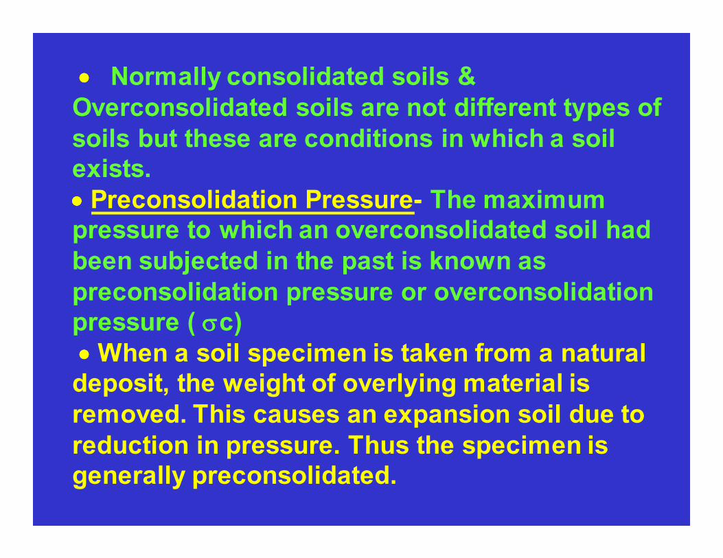
•••• Normally consolidated soils &
Overconsolidated soils are not different types of
soils but these are conditions in which a soil exists.
•••• Preconsolidation Pressure- The maximum pressure to which an overconsolidated soil had
been subjected in the past is known as
preconsolidation pressure or overconsolidation pressure ( σσσσc)
•••• When a soil specimen is taken from a natural deposit, the weight of overlying material is
removed. This causes an expansion soil due to
reduction in pressure. Thus the specimen is generally preconsolidated.

Final Settlement Of Soil Deposit In The Field •••• For computation of final settlement, the coefficient of volume change or compression index (Cc) is required. For time rate of computation, the Terzaghi’s theory is used. •••• Final settlement using coefficient of volume change : Let Ho = initial thickness of clay deposit.Consider a small element of thickness ∆z at depth z. ∆σ∆σ∆σ∆σ = effective pressure increment causing settlement. Then ∆∆∆∆H = mv Ho (∆∆∆∆σ ) Representing the final settlement as ∆∆∆∆sf & taking Ho = ∆∆∆∆z Thus, total settlement of the complete layer, alternatively
-
1
)........(2 i ) z ( i ) ( i ) mv ( ∆∂∆∑==
n
i
Sf
1) ( ........ Ho
,tan & mvboth
mv 0
−
−
−
∂∆=
∂∆
∆∂∆∫=∆∫=
mvSF
tconsareif
zHSFsf HoHo
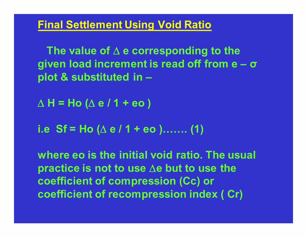
Final Settlement Using Void Ratio
The value of ∆∆∆∆ e corresponding to the
given load increment is read off from e – σ
plot & substituted in –
∆∆∆∆ H = Ho (∆∆∆∆ e / 1 + eo )
i.e Sf = Ho (∆∆∆∆ e / 1 + eo )YY. (1)
where eo is the initial void ratio. The usual
practice is not to use ∆∆∆∆e but to use the coefficient of compression (Cc) or
coefficient of recompression index ( Cr)

a) Normally Consolidated Soils - The compression index of
a normally considered soil is constant.
Cc σ0 + ∆σ
Sf = Ho Log 1+e0 10 σ0
b) Pre Consolidated Soils -
Cr σ0 + ∆σ Sf = Ho Log
1+e0 10 σ0
The above equation is applicable when (σ0 + ∆σ) < σc.


![[PPT]SHALLOW FOUNDATION - Home - Sri Venkateswara · Web viewSHALLOW FOUNDATION Introduction – Location and depth of foundation – Codal provisions – bearing capacity of shallow](https://static.fdocuments.us/doc/165x107/5aa985c27f8b9a9a188d0876/pptshallow-foundation-home-sri-venkateswara-viewshallow-foundation-introduction.jpg)
