BEARING CAPACITY OF FOOTINGS ON UNDRAINED SOFT CLAYS
62
BEARING CAPACITY OF FOOTINGS ON UNDRAINED SOFT CLAYS HANMO WANG 2018 A thesis submitted in partial fulfilment of The requirements for the award of Master of Engineering (Civil) Flinders University, Adelaide Australia
Transcript of BEARING CAPACITY OF FOOTINGS ON UNDRAINED SOFT CLAYS
BEARING CAPACITY OF FOOTINGS ON UNDRAINED SOFT CLAYS
HANMO WANG
2018
A thesis submitted in partial fulfilment of
The requirements for the award of
Master of Engineering (Civil)
Flinders University, Adelaide Australia

Declaration
I certify that this work does not incorporate without acknowledgement any material previously
submitted for a degree or diploma in any university: and that to the best of my knowledge and
belief it does not contain any material previously published or written by another person except
where due reference is made in the text.
Signed on this 15th October of 2018

i
ABSTRACT
The bearing capacity of foundaton is one of most important issue for soil and geotechnical
engineering. For foundation safety design, it is necessary to predict stability of footings under
saturated or unsaturated soil. The ultimate bearing capacity is the pressure at the base which
causes the foundation to failure and a sudden movement. The investigation of undrained bearing
capacity of shallow foundation on soft soil is limited in the past and most of data comes from
UK’s national soil test site, in Bothkennar, Scotland. In recent five years, Australian National
Filed Tesing Facility (NFTF) was constructed in Ballina, NSW for site investigation. A series of
in situ and laboratory tests were conducted on site in order to investigate the foundation behaviour
in terms of load settlement response, soil properties, etc.
During the last few decades, existing methods of estimating short term undrained bearing capacity
have been developed by various researchers. Limit equilibrium methods or empirical equations
are commonly used for estimating bearing capacity. However, uncertainties such as slope height,
distance between footing and excavation wall, soil properties are not considered, which make
calculations imprecisely.
In this study, foundation tests data from Ballina is analysed by using empirical bearing capacity
theory. The procedures include estimating undrained shear strength, ultimate bearing capacity,
effective settlement by using empirical bearing capacity equation and find the load -settlement
response for each type of test. A finite element analysis is used to simulate the foundation
geometry and load behaviour. The input data for numerical analysis such as Young’s modulus,
permeability, unit weight of soil, undrained shear strength should be determined from previous
foundation tests data. The load settlement response for both hand calculation and numerical
analysis are compared in this thesis.

ii
ACKNOWLEDGEMENTS
It is hard to complete this project without the help and support of the people around me. I would
like to thank my project supervisor Dr. QinHong Yu. His patience for answering questions,
urgent feedback, and kindly personality make me possible to accomplish this project.
I am grateful to my family, my parents for much support and encouragement of my studies.

iii
CONTENTS
Abstract ................................................................................................................................................ I
Acknowledgements ........................................................................................................................ II
1. INTRODUCTION ...................................................................................................................... 1
1.1 BEARING CAPACITY OF FOUNDATIONS ............................................................... 1
2. LITERATRURE REVIEW ........................................................................................................ 3
2.1 INTRODUCTION ........................................................................................................... 3
2.2 GENERALIZED BEARING CAPACITY THEORY .................................................... 3
2.3 REVIEW OF EARLY APPROACH .............................................................................. 4
2.3.1 Settlement ......................................................................................................... 9
2.4 PREVIOUS UNDRAINED BEAIRNG CAPACITY INVESTIGATION ................ 12
2.4.1 Upper bound theory analysis for square and rectangular footings ................................................................................................................................................... 12
2.4.2 Limit element analysis for bearing capacity ..................................... 12
2.4.3 Finite element analysis for bearing capacity .................................... 15
2.5 LITERATURE SUMMARY ........................................................................................ 16
3. BEARING CAPACITY OF LARGE-SCALE SHALLOW FOUNDATION IN BALLINA ................................................................................................................................................... 18
3.1 INTRODUCTION ......................................................................................................... 18
3.2 BACKGROUND OF THE SITE ................................................................................... 18
3.2.1 Foundation construction and loading blocks .................................... 20
3.3 UNDRAINED SHEAR STRNGTH RELATIONSHIP WITH ULTIMATE BEARING CAPACITY ............................................................................................................................... 21
3.3.1 Undrained shear strength for CPT ......................................................... 22
3.3.2 Undrained shear strength for SBP test................................................. 23
3.4 SOIL STIFFNESS AND ITS LINK TO SETTLEMENTS ......................................... 23
3.4.1 Vertical settlement ...................................................................................... 25
iv
3.5 FINITE ELEMENT ANALYSIS (FEA) ...................................................................... 25
3.5.1 Material input ............................................................................................... 26
3.6 PROJECT TIMELINE MANAGEMENT .................................................................... 26
4. BALLINA CASE RESULTS ................................................................................................... 29
4.1 RESULTS OF UNDRAINED SHEAR STRENGTH ............................................... 29
4.1.1 Undrained shear strength for CPT ......................................................... 29
4.1.2 Undrained shear strength for TC and TE ............................................. 30
4.1.3 Undrained shear strength for SBP test................................................. 32
4.1.4 Ultimate bearing capacity for each type of test ................................. 33
4.2 RESULTS OF SHEAR MODULUS AND SETTLEMENT ....................................... 34
4.2.1 Shear modulus results for Triaxial Test .............................................. 34
4.2.2 Shear modulus results for SBPM ............................................................ 37
4.2.3 Results of elastic shear modulus ............................................................ 38
4.2.4 Results of foundation settlement ........................................................... 39
4.2.5 Results of FEA ................................................................................................ 40
5. ANALYSIS AND DISCUSSION ............................................................................................. 43
5.1 Undrained shear strength and settlement ....................................................... 35
5.1.1 Load settlement response for empirical and numerical methods ................................................................................................................................................... 44
5.2 BOUNDARY IMPACY FOR NUMERICAL ANALYSIS .......................................... 45
5.3 BEARING CAPACITY EQUATIONS FOR UNDRAINED CLAY ........................... 46
6. CONCLUSIONS ....................................................................................................................... 50
7. REFERENCE ........................................................................................................................... 52

v
LIST OF FIGURES
Figure 1. Bearing capacity failure mechanism. ......................................................................... 2
Figure 2. Failure zones in Prandtl analysis (Prandtl, 1921) ....................................................... 5
Figure 3. Bearing capacity factor (Terzaghi and Peck, 1948) ..................................................... 6
Figure 4. Terzaghi's failure zones ............................................................................................... 7
Figure 5. Meyerhof's failure zone assumption ......................................................................... 8
Figure 6. Settlement components(Das et al, 2014) ................................................................ 10
Figure 7. Coefficients of μ0 and μ1 for vertical displacement ................................................ 11
Figure 8. Depth factor for different methods .......................................................................... 14
Figure 9. Shape factor for foundation ..................................................................................... 15
Figure 10.Site location (Science Direct, 2018) ......................................................................... 19
Figure 11. Foundation tests, Ballina region in NSW (Science Direct, 2018) ............................ 19
Figure 12. Test distribution (Ballina, 2013) .............................................................................. 20
Figure 13 Square footing dimensions ..................................................................................... 21
Figure 14.Beairng capacity factor (Terzaghi and Peck, 1948) .................................................. 22
Figure 15. Example of undrained shear strength for SBPM .................................................... 23
Figure 16. Deviatoric stress- strain graph for TC (Doherty, 2018) ........................................... 24
Figure 17. Soil stiffness graph for Poisson's ratio at 0.5 (Doherty and Deeks, 2003) .............. 25
Figure 18. Elastic perfectly model (Plaxis 2D, 2018) ................................................................ 26
Figure 19. Undrained shear strength profile for CPT ............................................................... 30
Figure 20. Undrained shear strength profile for TC ................................................................. 31
Figure 21. Undrained shear strength for TX ........................................................................... 32
Figure 22. Undrained shear strength for SBPM at 2.15 m....................................................... 32
Figure 23. Undrained shear strength versus depth for SBPM test .......................................... 33
Figure 24. Shear modulus profile of TX at depth 4.75 m ........................................................ 34
Figure 25. Shear modulus G10 profile ...................................................................................... 35
Figure 26. Shear modulus G50 profile ...................................................................................... 35
Figure 27. Shear modulus GMCCtx profile ................................................................................ 36
Figure 28. Pressuremeter data at varies depth ....................................................................... 37
Figure 29. Shear modulus for SBPM …… .................................................................................. 38
Figure 30. Load settlement for each soil stiffenss ................................................................... 40
Figure 31. Plan view of FEA model ........................................................................................... 41

vi
Figure 32. Mesh generating for FEA model ............................................................................. 41
Figure 33. Total deformation of foundation ............................................................................ 42
Figure 34. FEA load- settlement graph ................................................................................... 42
Figure 35. Load- settlement graph for hand caluclation and numerical analysis ................... 44
Figure 36. Failure mechanism for g = 0.34 m .......................................................................... 45
Figure 37. Failure mechanism for g = 0 m................................................................................ 46
Figure 38.Impact of the gap to calculate beaing capacity ....................................................... 46
Figure 39. Terzaghi's bearing capacity (Geotechnical Engineering Design, 2015) .................. 48
LIST OF TABLES
Table 1. Bearing capacity factor and shape factor from different researchers ...................... 16
Table 2. Project timeline ......................................................................................................... 27
Table 3. Undrained shear strength data for TC ...................................................................... 30
Table 4. Ultimate bearing capacity for each type of test ....................................................... 33
Table 5. Soil stiffness profile ................................................................................................... 36
Table 6. Shear modulus for each tyoe of test ......................................................................... 38
Table 7. Foundation settlements for TX and SBPM ................................................................ 39
Table 8. Foundation performance for UU test ....................................................................... 39
Table 9. Comparison of undrained shear strength and bearing capacity at foundation level.................................................................................................................................................. 43
Table 10. Settlemen for secant shear modulus ....................................................................... 44
Table 11. Prandtl's equation data ............................................................................................ 47
Table 12. Terzaghi's equation data (1) ..................................................................................... 47
Table 13. Terzaghi's equation data (2) ..................................................................................... 48

1
1 INTRODUCTION
In the last few decades there have been a lot of studies to investigate the foundations
performance in different soil conditions. Both empirical and numerical methods were
developed to improve the accuracy of site investigation. The ability to estimate ultimate bearing
capacity plays an important role in the foundation design. In the past theories, it has been
observed that the bearing capacity is commonly calculated using empirical equations or from
design charts which have been produced based on limit equilibrium or upper bound plasticity
calculation. Many of the existing methods can’t predict the ultimate bearing capacity precisely
due to the lack of considering important parameters of bearing capacity theory, such as the
distance of the footing from the slope, bearing capacity factors or soil properties. To understand
footing behaviours, it is important to analysis load-settlement response from empirical bearing
capacity theory and numerical analysis.
In this project, a prediction exercise for bearing capacity of shallow foundations under
undrained unconsolidated (UU) condition in soft clays is discussed. The site investigation was
conducted in Australian first National Field Testing Facility (NFTF) in Ballina, NSW. The site
has 6.5 hectares area, which offers a space to conduct a series of in situ and laboratory tests can
be conducted. The site tests include cone penetration tests (CPT), pressuremeter tests, triaxial
tests (TX) etc. The testing data was conducted by surveyors and uploaded to the web
application- datamap. Students are free to download relevant data from the application for both
study and practise target.
In this study, a geotechnical software- Plaxis 2D is used to conduct finite element analysis
(FEA) for Ballina Case. The numerical model was simulated based on the soil properties and
a range of variables were accounted for including footing size, slope height, soil types,
groundwater level, soil properties etc.
The main objectives of this research program are:
• To estimate the undrained bearing capacity of square footings on soft clay, taking
account of limit equilibrium theory and Terzaghi’s bearing capacity theory

1
• Determine parameters that influence the ultimate bearing capacity, which include
undrained bearing capacity factors, slopes between footing and excavation wall,
undrained shear strength
• Find the relationship between undrained shear strength and soil stiffness with its
foundation performance
• Investigate the load- settlement response from penetration, pressuremter, vane tests
• Compare the numerical analysis results with previous tests
1.1 BEARING CAPACITY OF FOUNDATIONS
The following discussion includes several definitions to facilitate the understand of later
chapters.
Bearing capacity is defined as the capability of the soil to counteract the pressure placed on
it. The ultimate bearing capacity is the pressure at the base which causes the foundation to
failure and a sudden settlement.
Bearing capacity failure mechanism: The failure model of bearing capacity is categorized
into three types, which is shown in Figure 1. The first mode of failure is called general shear
failure and extends through all three shearing zones. It often occurs for soils within a hard or
dense situation. The second mode is local shear failure and involves rupture of the soil only
immediately below the footing. It is often associated with a soft and stiffness soil. The third
type of failure is punching shear failure and occurs in very loose of soft soils. The process of
deformation of the footing involving compression of soil directly below the footing.
Unconsolidated undrained (UU) test is a triaxial compression test that accounts for the load
and drainage condition. In this test, the load applied on the sample is quick and the initial
specimen is undrained. The undrained shear strength can be obtained from effective shear
parameters- cohesion and friction angle. For UU test, friction angle (θ) = 0°, undrained shear
strength 𝑆𝑢 = deviator stress (𝜎1 − 𝜎3)/2.

2
Figure 1. Bearing capacity failure mechanism

3
2 LITERATURE REVIEW
2.1 INTRODUCTION
Foundation design consists of two important parts, ultimate bearing capacity of footings in soil,
and total settlement that the footing mobilizes. Soil properties and footing geometry are two
important factors that affect the bearing capacity of footings. Research on bearing capacity has
been investigated over one century with either theoretical or experimental methods. While a
satisfactory solution is approved only when both methods show the same results.
The previous studies developed multiple complex empirical equations to estimate the
undrained bearing capacity. However, the recent advancements in numerical methods for three-
dimensional footing analysis such as finite element method can rapidly improve the
experimental result.
In this chapter, most current methods of determining bearing capacity are reviewed. A
particular emphasis will be placed on discussing uncertainty that affect accuracy of calculating
bearing capacity in the last few sections and although some well-known and widely used theory
such as Terzaghi’s bearing capacity theory, Skempton’s bearing capacity factor, and relevant
modified theories are discussed. In the past, studies of undrained bearing capacity of
foundations on soft clay are limited in the literature. In cases where the soil properties vary
with depth, most of past theories cannot be implemented. Likewise, shape and depth factor for
foundations could not be estimated accurately. Therefore, it is necessary to compare the recent
studies using numerical analysis such as finite element method with empirical solutions to
define the accuracy of ultimate bearing capacity.
2.2 GENERALIZED BEARING CAPACITY THEORY
Probably the earliest recorded attempt to solve the problem of bearing capacity of strip
foundation was made by Rankine in 1857 (Abedin, 1986). He assumed that failure in the soil
is initiated by the formation of two wedges immediately beneath the foundation. While the
most known bearing capacity theory was originally developed for cohesionless soils by Pauker
(1850) and modified to accommodate cohesive by Bell (1915) and Prandtl (1921). Prandtl
developed bilinear failure surface into radial zones through the use of correction factors. The
most recent three failure zones are: a triangular active zone, a radial zone and a Rankine passive
4
zone (Terzaghi, et al., 1996). The triangular active zone is the result of active loading forces
from the foundation. The radial shear zone was derived assuming a log spiral slip surface in
cohesionless soils and is often called the transition zone (Perloff & Baron, 1976). The Rankine
passive zone is a result when pressures from loading are transferred to the confining soil via
the transition zone (Das, 2011).
The most early well-known bearing capacity theory was developed by Terzaghi (1943) and is
applicable for rough continuous foundations. He proposed two-dimensional plane strain model
to obtain bearing capacity for strip footing and later, he used three-dimensional mathematical
method to account for square and circular foundations. After that, Skempton (1951) found that
the depth of foundation impacts the bearing capacity factor, which found the relationship
between 𝑁𝑐 and ratio of 𝐷𝑓 /B. Several different methods exist in the literature to calculate
bearing capacity factors. The research presented in this report discussed the Hansen depth
factor, Vesic bearing capacity, Meyerhof shape coefficient etc. All these factors influence the
result of bearing capacity and should be compared.
2.3 REVIEW OF EARLY APPROACH
2.3.1 Previous studies
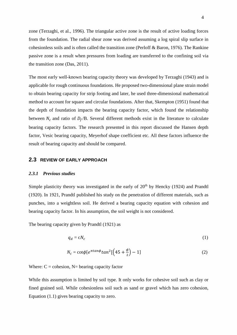
Simple plasticity theory was investigated in the early of 20th by Hencky (1924) and Prandtl
(1920). In 1921, Prandtl published his study on the penetration of different materials, such as
punches, into a weightless soil. He derived a bearing capacity equation with cohesion and
bearing capacity factor. In his assumption, the soil weight is not considered.
The bearing capacity given by Prandtl (1921) as
𝑞𝑑 = c𝑁𝑐 (1)
𝑁𝑐 = cot𝜙[𝑒𝜋𝑡𝑎𝑛𝜙𝑡𝑎𝑛2[(45 +𝜙
2) − 1] (2)
Where: C = cohesion, N= bearing capacity factor
While this assumption is limited by soil type. It only works for cohesive soil such as clay or
fined grained soil. While cohesionless soil such as sand or gravel which has zero cohesion,
Equation (1.1) gives bearing capacity to zero.
5
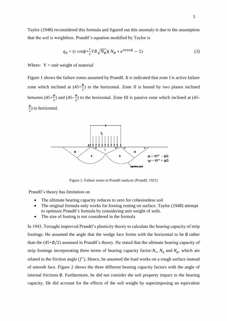
Taylor (1948) reconsidered this formula and figured out this anomaly is due to the assumption
that the soil is weightless. Prandtl’s equation modified by Taylor is
𝑞𝑑 = (c cot𝜙+1
2𝑌𝐵√𝑁𝜙)( 𝑁𝜙 ∗ 𝑒𝜋𝑡𝑎𝑛𝜙 − 1) (3)
Where: Y = unit weight of material
Figure 1 shows the failure zones assumed by Prandtl. It is indicated that zone I is active failure
zone which inclined at (45+𝜙
2) to the horizontal. Zone II is bound by two planes inclined
between (45+𝜙
2) and (45-
𝜙
2) to the horizontal. Zone III is passive zone which inclined at (45-
𝜙
2) to horizontal.
Figure 2. Failure zones in Prandtl analysis (Prandtl, 1921)
Prandtl’s theory has limitation on
• The ultimate bearing capacity reduces to zero for cohesionless soil
• The original formula only works for footing resting on surface. Taylor (1948) attempt
to optimize Prandtl’s formula by considering unit weight of soils.
• The size of footing is not considered in the formula
In 1943, Terzaghi improved Prandtl’s plasticity theory to calculate the bearing capacity of strip
footings. He assumed the angle that the wedge face forms with the horizontal to be ∅ rather
than the (45+∅/2) assumed in Prandtl’s theory. He stated that the ultimate bearing capacity of
strip footings incorporating three terms of bearing capacity factor:𝑁𝑐, 𝑁𝑞 and 𝑁𝑔, which are
related to the friction angle (𝑓′). Hence, he assumed the load works on a rough surface instead
of smooth face. Figure 2 shows the three different bearing capacity factors with the angle of
internal frictions ∅. Furthermore, he did not consider the soil property impact to the bearing
capacity. He did account for the effects of the soil weight by superimposing an equivalent
6
surcharge load q = Y𝐷𝑓. Although his principle of superposition is not correct, it leads to errors
not exceeding 17 to 20 percent for ∅ = 30° to 40°. This is equal to zero for ∅ = 0
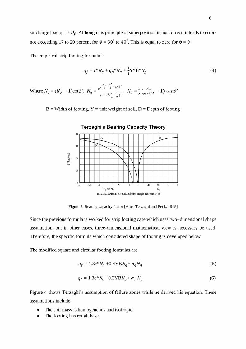
The empirical strip footing formula is
𝑞𝑓 = c*𝑁𝑐 + 𝑞𝑜*𝑁𝑞 + 1
2Y*B*𝑁𝑔 (4)
Where 𝑁𝑐 = (𝑁𝑞 − 1)cot∅′, 𝑁𝑞 = 𝑒
2(3𝜋4
−𝜃′
2)𝑡𝑎𝑛𝜃′
2𝑐𝑜𝑠2(𝜋
4+
𝜃′
2)
, 𝑁𝑔 = 1
2 (
𝐾𝑝
𝑐𝑜𝑠2𝜃′ − 1) 𝑡𝑎𝑛𝜃′
B = Width of footing, Y = unit weight of soil, D = Depth of footing
Figure 3. Bearing capacity factor [After Terzaghi and Peck, 1948]
Since the previous formula is worked for strip footing case which uses two- dimensional shape
assumption, but in other cases, three-dimensional mathematical view is necessary be used.
Therefore, the specific formula which considered shape of footing is developed below
The modified square and circular footing formulas are
𝑞𝑓 = 1.3c*𝑁𝑐 +0.4YB𝑁𝑔+ 𝜎𝑞𝑁𝑞 (5)
𝑞𝑓 = 1.3c*𝑁𝑐 +0.3YB𝑁𝑔+ 𝜎𝑞 𝑁𝑞 (6)
Figure 4 shows Terzaghi’s assumption of failure zones while he derived his equation. These
assumptions include:
• The soil mass is homogeneous and isotropic
• The footing has rough base

7
• The ground surface is horizontal
• The loading is vertical and symmetric
• Zone 1 represents elastic zone which moves downwards during footing failure
• Zone 2 represents radial shear zone bounded between ∅ and (45- 𝜙
2) to the horizontal
• Zone 3 represents linear shear zone once failure occurs at 45- 𝜙
2 to the horizontal
• The principle of superposition is applicable
Figure 4. Terzaghi’s Failure Zones
Although Terzaghi attempted to optimize Prandtl’s bearing capacity theory, his equation was
limited by experimentally condition. His theory does not provide the effects of footer depth,
load inclination factor or eccentricity, soil compressibility, water table and other factors.
In 1951, Skempton investigated Terzaghi’s bearing capacity factor and found that 𝑁𝑐 tends to
increase with depth in Terzaghi’s formula, where 𝑁𝑐 increases with increase in 𝐷𝑓/𝐵 ratio. He
also shows the relationship between ultimate bearing capacities with factor 𝑁𝑐 under undrained
conditions.
𝑞𝑓 = 𝑐𝑢𝑁𝑐 (7)
Where 𝑐𝑢 = undrained cohesion, 𝑞𝑓 = ultimate bearing capacity for saturated cohesive soil
under undrained conditions
The relationship between 𝑁𝑐 and 𝐷𝑓/𝐵 ratio is
For strip footing 𝑁𝑐 = 5(1+0.2𝐷𝑓
𝐵) ≤ 7.5 (8)
For square and circular footing 𝑁𝑐 = 6(1+0.2𝐷𝑓
𝐵) ≤ 9 (9)

8
For rectangular footing 𝑁𝑐 = 5(1+0.2𝐷𝑓
𝐵) (1+0.2
𝐵
𝐿) if
𝐷𝑓
𝐵 ≤ 2.5 (10)
𝑁𝑐 = 7.5(1+0.2𝐵
𝐿) if
𝐷𝑓
𝐵 > 2.5 (11)
Meyerhof (1963) refined Terzaghi’s bearing capacity equation and proposed further shape
coefficients in his theory. His theory considers the shear strength of soil in the overburden and
assumes the boundary of failure zone as a combination of logarithmic spiral failure surface and
a free surface.
He introduced shape factor, depth factor and inclination factor in his formula and developed
two equations to calculate vertical load bearing capacity and inclined load bearing capacity.
For vertical load:
𝑞𝑓 = c*𝑁𝑐*𝑠𝑐*𝑑𝑐 +𝜎𝑞*𝑁𝑞*𝑠𝑞*𝑑𝑞 +0.5*Y*B*𝑁𝑔*𝑠𝑔*𝑑𝑔 (12)
For Inclined load:
𝑞𝑓 = c*𝑁𝑐*𝑖𝑐*𝑑𝑐 + 𝜎𝑞*𝑁𝑞*𝑖𝑞*𝑑𝑞 + 0.5*Y*B*𝑁𝑔*𝑖𝑔*𝑑𝑔 (13)
Where: 𝑑𝑐, 𝑑𝑞, 𝑑𝑔 = Depth factor, 𝑖𝑐, 𝑖𝑞 , 𝑖𝑔 = Inclination factor
Figure 5. Meyerhof’s failure zone assumption
Meyerhof’s failure zone assumption is shown in Figure 5. Zone I is elastic zone and Zone II is
radial shear zone, as in Terzaghi’s assumption. While in Zone 3, the failure zones are assumed

9
above base of footings. Meyerhof’s assumption reflects that the shearing resistance of soil
above base of footings should be considered.
Brinch Hansen (1970) investigated the previous bearing capacity theory and developed his own
formulas for two separate cases of strength parameters; the friction angle ∅ >0, and ∅ = 0
(undrained clay). Hansen added ground and base factors in his formula in order to estimate
conditions for footing on slope.
For the case: ∅ >0
𝑞𝑓 = c𝑁𝑐𝑆𝑐𝑑𝑐𝑖𝑐𝑏𝑐𝑔𝑐 + 𝑞𝑜𝑁𝑞𝑆𝑞𝑑𝑞𝑖𝑞𝑏𝑞𝑔𝑞+0.5YB𝑁𝑦𝑆𝑦𝑑𝑦𝑖𝑦𝑏𝑦𝑔𝑦 (14)
Where 𝑞𝑜 = effective overburden pressure, 𝑆𝑐, 𝑆𝑞 , 𝑆𝑦 = Shape factors, 𝑖𝑐, 𝑖𝑞, 𝑖𝑦 = inclination
factors, 𝑑𝑐, 𝑑𝑞, 𝑑𝑦 = depth factors
For the case: ∅ =0
𝑞𝑓 = (𝜋 + 2) 𝑠𝑢(1+𝑠𝑠𝑢+𝑑𝑠𝑢-𝑖𝑠𝑢-𝑏𝑠𝑢- 𝑔𝑠𝑢) + 𝑞𝑜 (15)
Where 𝑠𝑠𝑢 = 0.2𝐵
𝐿 , 𝑑𝑠𝑢 = 0.4
𝐷
𝐵 for D ≤ B, 𝑑𝑠𝑢 = 0.4 𝑡𝑎𝑛−1(
𝐷
𝐵) for D > B, 𝑖𝑠𝑢 = 0.5-
0.5√1 −𝑄𝑡𝑟−𝐵
𝑐𝑎𝐴𝑓
He suggested the use of Prandtl and Reissner’s values for 𝑁𝑐 and 𝑁𝑞, and a value of 𝑁𝑦 was
proposed as:
𝑁𝑦 = 1.8 (𝑁𝑞 − 1)tan∅ (16)
Balla (1962) assumed a failure surface, combined with a circular arc and a tangential straight
line
2.3.2 Settlement
The settlement of a footing under loading is one of the most important criteria in its structural
design. There are many factors which influence the settlement of a foundation. These include
the ultimate bearing pressure, the soil layer thickness under the footing and the overburden
surcharge.

10
The total settlement, 𝑆𝑡, that can occur underneath a footing, include three components. The
equation is shown as:
𝑆𝑡 = 𝑆𝑖+𝑆𝑐+𝑆𝑠 (17)
Where 𝑆𝑖 is immediate settlement, 𝑆𝑐 is primary settlement, 𝑆𝑠 is secondary settlement.
Total soil settlement can be represented by the elastic and consolidation deformation. Figure 6
shows the deformation trend for settlements, which can be identified as three conditions.
Stage 1 is initial compression condition which make deformation rapidly. On the second stage,
primary settlement occurs, and water pressure dissipates during the period. Second settlement
occurs after the complete dissipation of excess pore water pressure.
Figure 6. Settlement components (Das et al, 2014)
Total soil settlement can also represent by the sum of elastic settlement and consolidation
settlement.
Most of the settlement of foundations on saturated cohesive soil is due to consolidation and
associated dissipation of excess pore-water pressure. The vertical settlement of a thin soil layer
of finite thickness subjected to uniform loading is:
𝑆𝑖 = 𝜇0𝜇1𝑞𝐵
𝐸 (18)

11
Where
𝜇0 = Coefficient depending on depth of embedment
𝜇1 = Coefficient depending on layer thickness and shape of the loaded area
E = Young’s modulus
B = Width of foundation
Figure 7. Coefficients of 𝜇0 and 𝜇1 for vertical displacement
In a clay layer, primary settlement always takes a couple of months or even years to complete
due to the soil properties. Total stress analysis uses the undrained shear strength, 𝑠𝑢, which can
be approximated using field tests.
In clays, primary settlement takes year to complete during the project, but varies with other
factors such as loading rate or duration of loading. Normal Consolidated clay primary
settlement is
𝑆𝑐 = ∆𝑒
1+𝑒𝑜 𝐻0 (19)

12
Where ∆𝑒 = Change in void ratio= 𝐶𝑐log(𝜎′
𝑜+∆𝜎
𝜎′𝑜
)
𝑒𝑜 = Initial void ratio
𝐻0 = Height of sample
Overconsolidated clay occurs when the present overburden pressure is less than the soil has
experienced in the past. The clay properties are mainly dependent on the initial vertical
effective stress, 𝜎′𝑣𝑜, and the preconsolidation pressure, 𝜎′
𝑐. The preconsolidation pressure is
the maximum previously applied stress. The over consolidation ratio, OCR has a relationship
with ratio of initial vertical effective stress and preconsolidation pressure.
OCR = 𝜎′
𝑐
𝜎′𝑣𝑜
(20)
2.4 PREVIOUS UNDRAINED BEARING CAPACITY INVESTIGATION
2.4.1 Upper bound theory analysis for square and rectangular footings
Michalowski (2001) used limit analysis to calculate the bearing capacity of square and
rectangular footings and compare with early empirical results. He simplified formula of rate of
work dissipation to conduct limit analysis of three-dimensional problems. It was found that
internal friction has significantly impact for shape factors. For large internal friction angles (Ꝕ>
16°) the shape factors are rapidly increasing when the footing aspect ratio drops to 1. He
obtained a bearing capacity factor of 6.56 for square footing which is 10% higher than the
Meyerhof and de Beer’s proposal. The results indicate that Meyerhof and de beer’s calculation
lack of systematic experimental test, validation of shape factors derived can’t be reliably.
Therefore, the existing proposals for shape factors are probably conservative. Furthermore, the
author suggested that kinematic admissibility is a significant problem for three- dimensional
analysis rather than two dimensional problems. Consequently, the estimation of shape factors
by upper bound theory are likely overestimated (particularly for large friction angle).
Therefore, numerical analysis which do not constraint pattern deformation is recommended to
improve solutions for square and rectangular footings.

13
2.4.2 Limit element analysis for bearing capacity
In the previous review, it can be found that the empirical strip footing formula developed by
Terzaghi in 1943 make designers were able to find a foundation framework and develop the
former’s work. The first exact solution for bearing capacity factor 𝑁𝑐 was found by Prandtal
(1921) by considering a strip footing with shear strength 𝑠𝑢. After that, a rigid circular footing
resting on frictionless soil was investigated by Eason& Shield (1960) by using the Haar-Von
Karman hypothesis and slip-line method. While the exact solutions of square and rectangular
footings placed at some depth within the soil are not found, instead engineers developed critical
factors from theoretical equations to solve these problems. Critical factors such as shape factors
and depth factors could not be obtained precisely.
Salagado, et al (2004) investigated the bearing capacities of different shape foundations in clay
and used limit element analysis to find the results of critical factors for different foundations.
The limit analysis was proved as a tool to solve the bearing capacity problems and stability
problems since Hill (1951) and Drucker et al (1951) published their breaking upper and lower
plasticity theory. The lower bound theorem emphasizes that the collapse does not happened for
a statically admissible stress field. Conversely, upper bound theorem states that collapse is
already under way or imminent for an admissible velocity field. These two virtual work
equations are represented as:
ʃ𝑠𝑇𝑖𝐿𝑣𝑖dS + ʃ𝑣𝑋𝑖
𝐿𝑣𝑖dV = ʃ𝑣σ𝑖𝑗𝐿έ𝑖𝑗dV ≤ ʃ𝑣𝐷έ𝑖𝑗dV = ʃ𝑣σ𝑖𝑗έ𝑖𝑗dV (21)
ʃ𝑠𝑇𝑖𝑢𝑣𝑖
𝑢dS + ʃ𝑣𝑋𝑖𝑢𝑣𝑖
𝑢dV = ʃ𝑣σ𝑖𝑗𝑢έ𝑖𝑗
𝑢dV = ʃ𝑣𝐷έ𝑖𝑗
𝑢dV ≥ ʃ𝑣σ𝑖𝑗έ𝑖𝑗
𝑢dV (22)
Where σ𝑖𝑗𝐿 = statically admissible stress field,
σ𝑖𝑗 = stress field
έ𝑖𝑗 = strain rate field
𝑣𝑖 = velocity field
𝑣𝑖𝑢 = kinematically admissible velocity field
For strip footings, the bearing capacity is calculated for various depths of embedment. It is
clear that the larger bearing capacities at larger aspect ratio due to deeper foundations mobilize
14
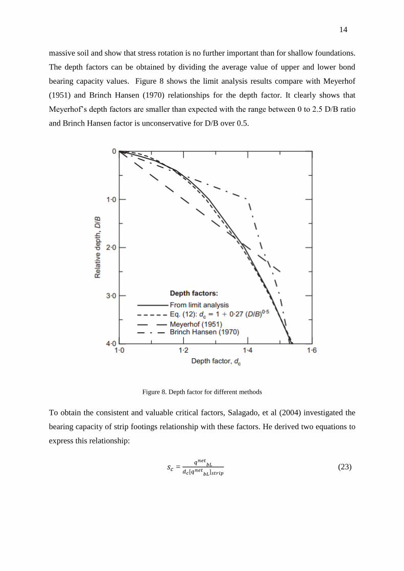
massive soil and show that stress rotation is no further important than for shallow foundations.
The depth factors can be obtained by dividing the average value of upper and lower bond
bearing capacity values. Figure 8 shows the limit analysis results compare with Meyerhof
(1951) and Brinch Hansen (1970) relationships for the depth factor. It clearly shows that
Meyerhof’s depth factors are smaller than expected with the range between 0 to 2.5 D/B ratio
and Brinch Hansen factor is unconservative for D/B over 0.5.
Figure 8. Depth factor for different methods
To obtain the consistent and valuable critical factors, Salagado, et al (2004) investigated the
bearing capacity of strip footings relationship with these factors. He derived two equations to
express this relationship:
𝑠𝑐 = 𝑞𝑛𝑒𝑡
𝑏𝐿
𝑑𝑐[𝑞𝑛𝑒𝑡𝑏𝐿]𝑠𝑡𝑟𝑖𝑝
(23)
15
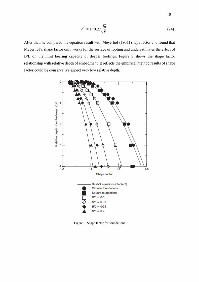
𝑑𝑐 = 1+0.27√𝐷
𝐵 (24)
After that, he compared the equation result with Meyerhof (1951) shape factor and found that
Meyerhof’s shape factor only works for the surface of footing and underestimates the effect of
B/L on the limit bearing capacity of deeper footings. Figure 9 shows the shape factor
relationship with relative depth of embedment. It reflects the empirical method results of shape
factor could be conservative expect very low relative depth.
Figure 9. Shape factor for foundations
16
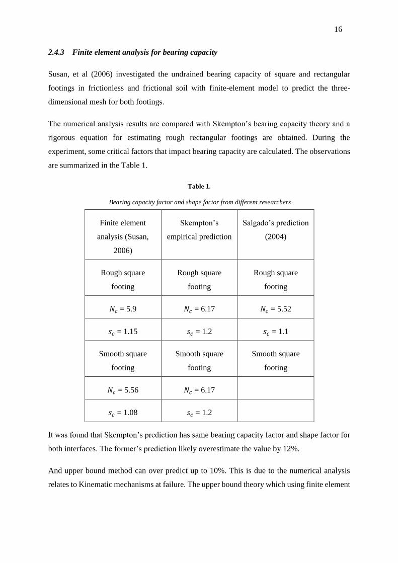
2.4.3 Finite element analysis for bearing capacity
Susan, et al (2006) investigated the undrained bearing capacity of square and rectangular
footings in frictionless and frictional soil with finite-element model to predict the three-
dimensional mesh for both footings.
The numerical analysis results are compared with Skempton’s bearing capacity theory and a
rigorous equation for estimating rough rectangular footings are obtained. During the
experiment, some critical factors that impact bearing capacity are calculated. The observations
are summarized in the Table 1.
Table 1.
Bearing capacity factor and shape factor from different researchers
Finite element
analysis (Susan,
2006)
Skempton’s
empirical prediction
Salgado’s prediction
(2004)
Rough square
footing
Rough square
footing
Rough square
footing
𝑁𝑐 = 5.9 𝑁𝑐 = 6.17 𝑁𝑐 = 5.52
𝑠𝑐 = 1.15 𝑠𝑐 = 1.2 𝑠𝑐 = 1.1
Smooth square
footing
Smooth square
footing
Smooth square
footing
𝑁𝑐 = 5.56 𝑁𝑐 = 6.17
𝑠𝑐 = 1.08 𝑠𝑐 = 1.2
It was found that Skempton’s prediction has same bearing capacity factor and shape factor for
both interfaces. The former’s prediction likely overestimate the value by 12%.
And upper bound method can over predict up to 10%. This is due to the numerical analysis
relates to Kinematic mechanisms at failure. The upper bound theory which using finite element
17
analysis indicates a failure mechanism that has fourfold symmetry. While the optimum
mechanisms for a square footing that has only twofold symmetry.
2.5 SUMMARY
The past studies on predicting bearing capacity commonly used empirical equations based on
plasticity theory or empirical calculation. Traditional bearing capacity theory does not take
important factors that affect bearing capacity into account. In recent studies, researchers start
to consider these parameters such as the slope height, distance of the footing from the slope
and the soil properties with a combination of numerical analysis such as two-dimensional
footing analysis to reduce the uncertainty of bearing capacity.
The literature review has discussed the following points that are relevant to the project.
1. The internal friction angle has significantly impact for shape factors.
2. The shape factor can’t be calculated precisely by using upper bond theory
(Michalowski, 2001)
3. The value of ultimate bearing capacity relates to the aspect ratio, and stress rotation
has less impact to the shallow foundations.
4. It is proved that rough footing has larger bearing capacity than smooth footings.
5. Meyerhof’s depth factor is conservative with the D/B ratio, however it only works for
surface footings or very shallow footings.
6. Brinch Hansen depth factor is conservative with the D/B ratio over 0.5.
7. Based on finite element analysis, failure mechanisms for square footings exhibit
fourfold symmetry.
18
3 BEARING CAPACITY OF LARGE-SCALE
SHALLOW FOUNDATION IN BALLINA
3.1 INTRODUCTION
The investigation of undrained bearing capacity of footings on soft clay is an important issue
for foundation design. In this chapter a series of in situ and laboratory tests conducted in
Australian National Field-Testing Facility (NFTF) at Ballina are analysed to predict the
response of foundations under unconsolidated and undrained (UU) loading. Results of large-
scale shallow foundation of UU tests are limited in the literature, and most of them were tested
at UK’s national soft soil test site in Bothkennar. To improve the accuracy of determining soil
properties, a full-scale embankment, with both in situ and laboratory tests tools, was
constructed and instrumented at Ballina in 2013. The instrumentations include measurement of
horizontal and vertical loadings, deformations and pore pressure over time. Two rigid square
foundations were loaded vertically to failure under UU condition. The foundation response is
recorded and load- settlement graph indicates its bearing capacity behaviour.
It has been found that many bearing capacity theories are not rigorous and contain lots of
uncertainties such as the boundaries between footings and excavation wall, slope height, or the
soil properties. In recent twenty years, researchers explored professional software to solve
complex geotechnical problems based on the development of the computer. The finite element
analysis (FEA) is one of geotechnical modelling methods to investigate the specific issues. In
this study, numerical analysis apply on Plaxis 2D is used to calculate the bearing capacity of
footings. By using this software, a predicted load settlement response can be identified.
3.2 BACKGROUND OF THE SITE
The test site is located at Ballina in NSW, Australia as shown in the map in Figure 10. The site
is founded to be 6.5 Ha in area and lies on the Richmond river. Through the observation of
boreholes, the groundwater level is about 1.0 m depth (0.5m AHD). The site is comprised of
1.5 m of alluvial clayey sand, underlain by 11 m soft estuarine clay. Photo is shown in Figure
11. A comprehensive site investigation has been conducted by geotechnical engineers
involving drilling 15 boreholes and collecting soil samples by test apparatus. A range of field
tests have been conducted in the Figure 12, which include cone Penetration tests (CPT), triaxial

19
Compression (TC) & triaxial extension (TE) test, and self- boring Pressuremeter test (SBPMT).
There are similarities existing between Bothkennar and Ballina site. For example, the site
condition and foundation geometry are extremely similar for both sites. The Bothkennar site is
comprised of 2 m of clay and silt, underlain by few meters marine clay. The observed
foundations have similar dimensions and same testing procedures in order to compare the
results of tests.
Figure 10. Site location (Science Direct, 2018)
Figure 11. Foundation tests, Ballina region in NSW

20
Figure 12. Tests distribution (Ballina, 2013)
3.2.1 Foundation construction and loading blocks
The early stage of preparing testing apparatus include build and cast tested foundations and
loading blocks. In this case, square foundations with 1.8 m length and 0.6 m thick were cast
1.5 m below ground level. The configuration and ground water level of footings is shown in
Figure 13. The relevant excavating procedures include excavate a 2.4 × 1.5 𝑚2 construction
space. After the excavation, the foundation was cast in concrete with 32 MPa and a
surrounding timber formwork was built to against the concrete pressure. The loading blocks
are made with same plan dimension of square foundations but 0.425 m height. Each

21
reinforced concrete block has weight about 3.3 tonnes with average unit weigh of 24 KN/𝑚3,
which indicates that each block led to an increasing of 10 KPa bearing pressure.
Figure 13. Square footing dimensions
3.3 UNDRAINED SHEAR STRENGTH RELATIONSHIP WITH ULTIMATE BEARING
CAPACITY
Bearing capacity is defined as the capacity of the soil to support the foundation. To calculate
the ultimate bearing capacity, it is important to find the soil properties through in situ tests and
laboratory tests. The soil parameters such as strength, stiffness and permeability can be
determined through these tests. In this case, a modified Terzaghi’s bearing capacity equation
is used to represent the undrained shear strength and its relationship to bearing capacity.
𝑄𝑢 = A (𝑁𝑐𝑆𝑢 + 𝑞𝑁𝑞) (25)
Where A = Area of the foundation, 𝑁𝑐, 𝑁𝑞 = bearing factor, q= surcharge adjacent to the
foundation
The Terzaghi’s bearing capacity factor is related to the internal friction angle. In undrained
condition, the increase in pore pressure occurs at the same rate as the application of stress.
Therefore, the internal friction angle (∅) is equal to zero, which leads to 𝑁𝑐 = 6 and 𝑁𝑞 = 0 from
chart. A straight relationship between ultimate bearing capacity and undrained shear strength can be
obtained for this case.
𝑄𝑢 = 19.44𝑆𝑢 (26)

22
Figure 14. Bearing capacity factor (Terzaghi and Peck, 1948)
Undrained shear strength can be estimated through a range of in situ and laboratory tests,
which include CPT, SBPM, TXC and TXE tests.
3.3.1 Undrained shear strength for Cone penetration tests
Geotechnical parameters can be estimated in cone penetration tests depending on soil types.
These parameters include total cone resistance, penetration pore pressure, empirical cone
factor. The total cone resistance is shown in the following equation,
𝑞𝑡 = 𝑞𝑐 + (1-a) 𝑢2 (27)
Where, 𝑞𝑡 = total cone resistance, 𝑞𝑐 = Cone resistance, 𝑢2 = penetration pore pressure
The undrained shear strength can be calculated in terms of the cone resistance and empirical
cone factor.
𝑆𝑢 =( 𝑞𝑡 - 𝑢2 ) / 𝑁𝑘 (28)
Where, 𝑆𝑢 = undrained shear strength, 𝑁𝑘 = empirical cone factor
23
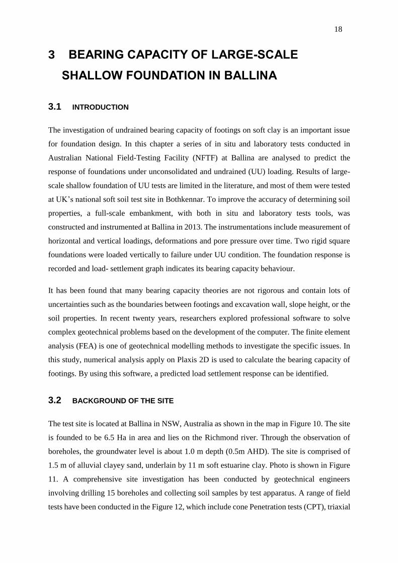
3.3.2 Undrained shear strength for self-boring pressuremeter test
Various methods have been used for calculating undrained shear strength for pressurementer
tests. Most common method is to use Gibson & Anderson (1961) approach for interpreting a
Menard pressuremeter test (Gaone, 2016). Undrained shear strength can be simplified as a
gradient of cavity pressure against logarithm of the cavity strain.
Figure 15. Example of undrained shear strength for SBPM
3.4 SOIL STIFFNESS AND ITS RELATIONSHIP TO SETTLEMENTS
In this section, shear modulus can be determined through Triaxial compression tests and self-
boring pressuremeter tests. Shear modulus is determined as the rate of shear stress to the shear
strain. It is an important factor to observe the deformation of foundations. By selecting three
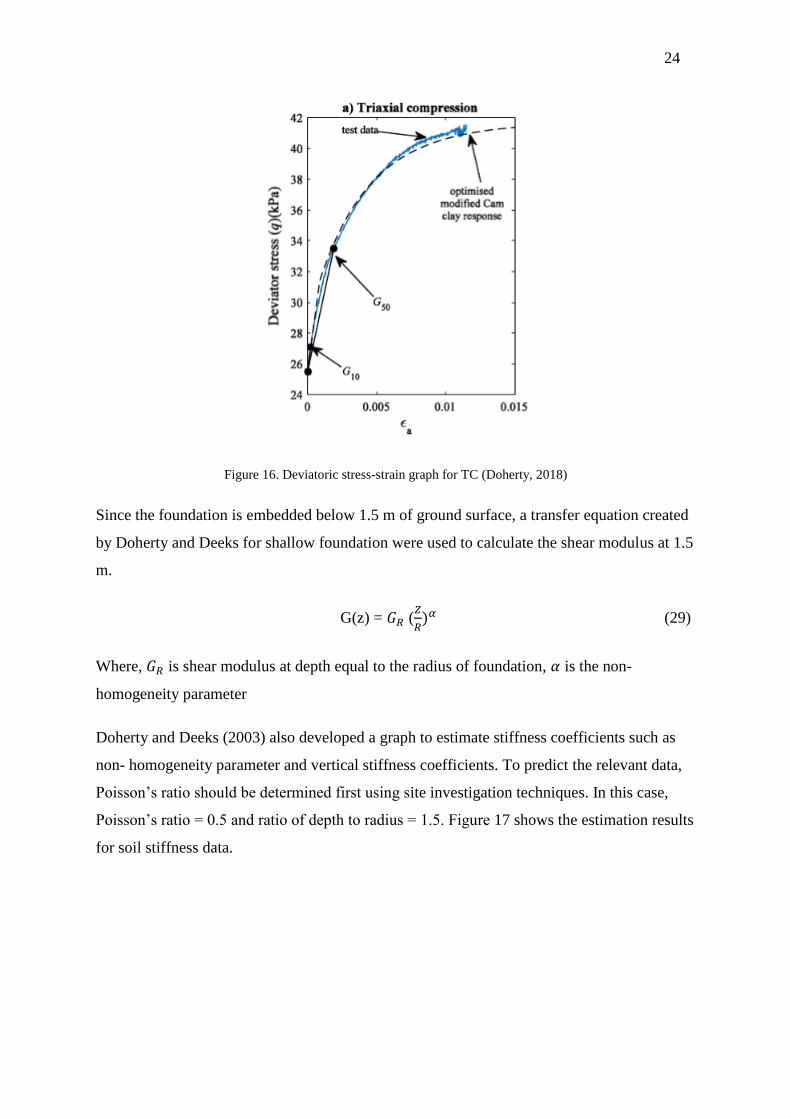
significant points on deviatoric stress (q) versus axial strain (Ɛ𝑎) graph- 𝐺10, 𝐺50, 𝐺𝑀𝐶𝐶𝑡𝑥, best
fit linear shear modulus versus depth graph can be obtained. Each point represents 10%, 50%
and optimized of the total change in deviatoric stress. Figure 16 shows one example of triaxial
compression test data at 4.75 m depth. Three points for stress-strain rate with varies depth are
applied to generate the shear modulus versus depth graphs.
24
Figure 16. Deviatoric stress-strain graph for TC (Doherty, 2018)
Since the foundation is embedded below 1.5 m of ground surface, a transfer equation created
by Doherty and Deeks for shallow foundation were used to calculate the shear modulus at 1.5
m.
G(z) = 𝐺𝑅 (𝑍
𝑅)𝛼 (29)
Where, 𝐺𝑅 is shear modulus at depth equal to the radius of foundation, 𝛼 is the non-
homogeneity parameter
Doherty and Deeks (2003) also developed a graph to estimate stiffness coefficients such as
non- homogeneity parameter and vertical stiffness coefficients. To predict the relevant data,
Poisson’s ratio should be determined first using site investigation techniques. In this case,
Poisson’s ratio = 0.5 and ratio of depth to radius = 1.5. Figure 17 shows the estimation results
for soil stiffness data.

25
Figure 17. Soil stiffness graph for Poisson’s ratio at 0.5 (Doherty and Deeks, 2003)
3.4.1 Vertical settlement
In this section, total settlement can be estimated once the above parameters are obtained.
U = 𝑄
𝐺𝑅R𝐾𝑣 (30)
Where, U = Total vertical settlement, Q= ultimate bearing capacity, R = radius of foundation,
𝐾𝑣 = vertical stiffness coefficients
Once the settlement is calculated, it is supposed to find efficient settlements under working
loads. The total vertical settlement is significantly affected by inefficient loading after failure.
To investigate the reasonable load-settlement response, settlements of 25%, 50% of ultimate
failure load (𝑢25, 𝑢50) are estimated.
3.5 FINITE ELEMENT ANALYSIS (FEA)
A suitable foundation design requires reasonable estimation in terms of soil properties, ultimate
bearing capacity, and interaction between footing geometry and soil parameters. Therefore, it
is essential to identify numerical analysis inputs efficiency to avoid unexpected results. In this
case, Plaxis 2D is used to simulate the square footing behaviour in unconsolidated undrained
condition. An axisymmetric model using 15-noded elements was created. The two different
layers of soil with 1.5 m clayey sand and 8.5 m estuarine clay was modelled to represent the
crust and underlaying soils. The excavation and foundation geometry are shown in Figure 18.

26
The axisymmetric model simulates the foundation and excavation pit as circle, which means
the boundaries of both pits can be calculated as radius. The foundation and excavation have
radius of 1.013 m and 1.35m, which has a gap about 0.34m.
3.5.1 Material input
Material input includes determination of material model, soil unit weight, Young’s modulus,
undrained shear strength. The crust layer was selected as a Mohr- Coulomb model, which is
also called linear elastic perfectly model. Mohr-Coulomb model is based on Hook’s law of
isotropic elasticity, which relate the stress rate to the elastic strain rates. This is shown in Figure
18. The strain rates can be either elastic or plastic. The Young’s modulus 3MPa and undrained
shear strength 24 kPa are obtained through CPT. The average unit weight of sand is 17 KN/𝑚2,
Poisson’ ratio is determined as 0.495 (0.5) for undrained material due to the strain is small
enough. Similar as crust layer, the soft clay was modelled as a Tresca elastic plastic model with
8.5 m thickness. The unit weight is 14 KN/𝑚2, and 11.2 kPa as undrained shear strength.
Figure 18. Elastic perfectly model (Plaxis 2D, 2018)
3.6 PROJECT TIMELINE MANAGEMENT
In this section, a detailed timeline for the project is discussed to conduct the project in a realistic
and feasible way. Since the project consists of few activities, such as topic selection, proposal
presentation, literature review, supervisor meeting, Expo poster etc, it is important to report
each period progress to make sure the whole project can be accomplished on time. The project
starts from March of 2018 and finishes at 15th of October. It includes Project proposal

27
presentation, literature investigation, Project results presentation, Expo poster, and final thesis.
However, the project takes almost nine months to complete. During this period, the time
management is necessary for student to update realistic course performance.
In semester 1, the task was focused on the selection of project topic and feasibility studies.
After selecting the project topic and identifying the reliability of the references, a proposal
presentation on mid break of semester one. This presentation contains a feasibility study of
current state of knowledge and make students understand the project plan of task in next
semester. Student is supposed to finish their literature review by the end of semester one.
In semester two, the study focuses on experimental results such as empirical hand calculation
results and numerical analysis results. It is supposed to meet with supervisor once a week to
solve questions. Since this project has no experimental tasks, the major work focuses on
theoretical performance, which include investigate geotechnical issues relevant to given in situ
and laboratory data and Plaxis 2D (numerical analysis). A project results presentation is
planned to be presented in week 7 to evaluate the understanding of the topic. In the presentation,
students are supposed to display their investigation results to audience and prove why it is
worth to do this topic. An Expo Poster is necessary to be finished in week 11. Meanwhile, the
edition of the final report is supposed to be done.
Table 2.
Project timeline
Tasks Name Duration (days) Start Finish
Project selection 12 26/02/18 10/03/18
Proposal presentation 30 10/03/18 10/04/18
Literature review 18 10/04/18 21/07/18
Case study
investigation
70 21/07/18 14/09/18
Results seminar 2 17/09/18 18/09/18

28
Optimization results
data
10 18/09/18 28/09/18
Expo Poster 2 16/10/18 17/10/18
Final thesis submission 61 15/08/15 15/10/15

29
4 BALLINA CASE RESULTS
In this part, details of the case study results are shown both hand calculation and numerical
results. The first part of results includes Terzaghi’s bearing capacity calculation in terms of
foundation settlement. The second part of results indicate numerical model of load- settlement
response by finite element analysis. Meanwhile, both empirical results and numerical results
would compare with the measured foundation performance values (UU data).
4.1 RESULTS OF UNDRAINED SHEAR STRENGTH
Undrained shear strength can be obtained from a couple of in situ tests and laboratory tests.
These tests include triaxial compression test (TC), triaxial extension test (TE), cone penetration
test (CPT) and self- boring pressuremeter test (SBPM).
4.1.1 Undrained shear strength for CPT
Table 3 shows the results of undrained shear strength with varies depth in cone penetration
test. Undrained shear strength is calculated by using rate of effective cone resistance and
given empirical cone factor. Figure 19 shows the undrained shear strength versus depth graph
for CPT. The linear line is plotted to represent the trend of graph and also helpful to find the
undrained shear strength at foundation level (1.5 m below the ground surface). For the CPT
profile, the empirical cone factor is given as 12.2 from in situ test data (Kell, 2014).
𝑆𝑢 =( 𝑞𝑡 - 𝑢2 ) / 𝑁𝑘𝑡 (31)
Where 𝑆𝑢 = Undrained shear strength, (𝑞𝑡 - 𝑢2) = Effective cone resistance,
𝑁𝑘 = Empirical cone factor
The depth of soil depends on the thickness of layers. In this case, the first layer is clayey silty
sand with 1.5 m thickness and second layer is estuarine clay about 12 m. Based on the
excavating level at 1.5 m below the ground, the total 10 meters depth is enough for site
investigation.

30
Figure 19. Undrained shear strength profile for CPT
4.1.2 Undrained shear strength from TC and TE
The triaxial compression and triaxial extension tests data are given below. In an
unconsolidated undrained condition, the friction angle is zero due to the effective stress will
always be the same. The best linear line graph related to undrained shear strength with depth
are shown in Fig 20 and Fig 21.
Table 3.
Undrained shear strength data for TC
0.000
1.000
2.000
3.000
4.000
5.000
6.000
7.000
8.000
9.000
10.000
0 5 10 15 20 25 30
Dep
th (
m)
Undrained shear strength (kPa)
CPT
Depth (m) Unconfined compressive
strength (KPa)
Undrained shear strength (KPa)
D 𝑞𝑢 𝑆𝑢 = 𝑞𝑢 / 2
1.76 14.6 7.3
1.96 18.5 9.25
2.37 27.24 13.62
3.05 23.44 11.72

31
Figure 20. Undrained shear strength profile for TC
0
2
4
6
8
10
12
0 2 4 6 8 10 12 14 16 18 20
Dep
th (
m)
Undrained shear strength (kPa)
Triaxial Compression
4.76 22.78 11.39
4.96 28.46 14.23
5.4 26.22 13.11
5.58 29.12 14.56
6.53 30.06 15.03
7.38 8.72 17.44
7.88 34.3 17.15
10.34 33.6 16.8

32
Figure 21. Undrained shear strength profile for TX
4.1.3 Undrained shear strength for pressuremeter test
The undrained shear strength for SBPM can be determined in elastic plastic model following
by Gibson & Anderson (1961) approach. Undrained shear strength is the gradient of cavity
pressure to logarithm cavity strain. The following graph shows the undrained shear strength
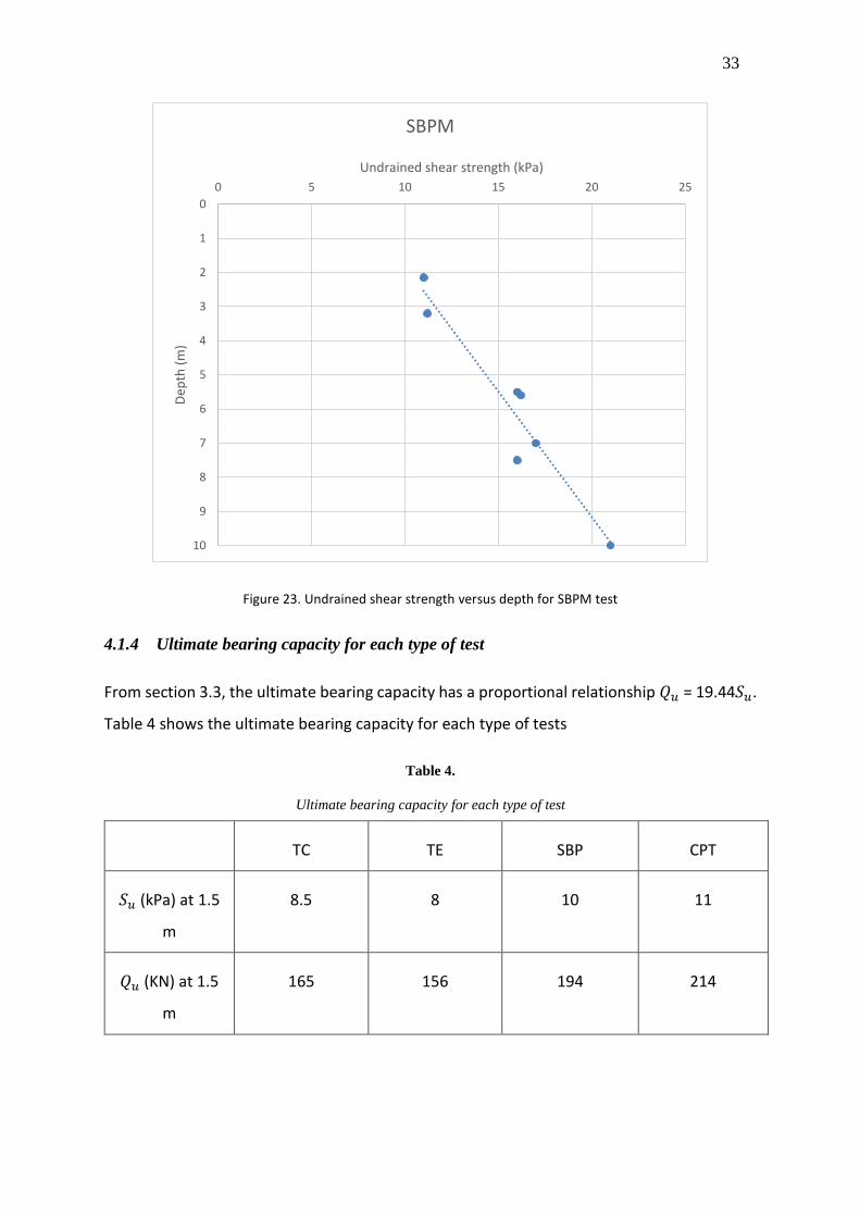
profile at depth 2.15 m below ground surface. Figure 22 represents the shear strength versus
depth graph, which 𝑆𝑢 at foundation level is estimated as 10 KPa.
Figure 22. Undrained shear strength profile for SBPM at 2.15m
0
2
4
6
8
10
12
0 5 10 15 20 25
Dep
th (
m)
Undrained shear strength (kPa)
Triaxial Extension
33
Figure 23. Undrained shear strength versus depth for SBPM test
4.1.4 Ultimate bearing capacity for each type of test
From section 3.3, the ultimate bearing capacity has a proportional relationship 𝑄𝑢 = 19.44𝑆𝑢.
Table 4 shows the ultimate bearing capacity for each type of tests
Table 4.
Ultimate bearing capacity for each type of test
TC TE SBP CPT
𝑆𝑢 (kPa) at 1.5
m
8.5 8 10 11
𝑄𝑢 (KN) at 1.5
m
165 156 194 214
0
1
2
3
4
5
6
7
8
9
10
0 5 10 15 20 25D
epth
(m
)Undrained shear strength (kPa)
SBPM

34
4.2 RESULTS OF SHEAR MODULUS AND SETTLEMENT
This section covers the shear modulus and foundation settlement results for Ballina case. The
shear modulus can be estimated from TX and SBPM with multiply methods. The foundation
settlement found following a relationship with shear modulus, ultimate bearing capacity and
stiffness coefficients.
4.2.1 Shear modulus results for triaxial test
The interpretation of soil stiffness has shown in section 3.4. Three significant points 𝐺10, 𝐺50,
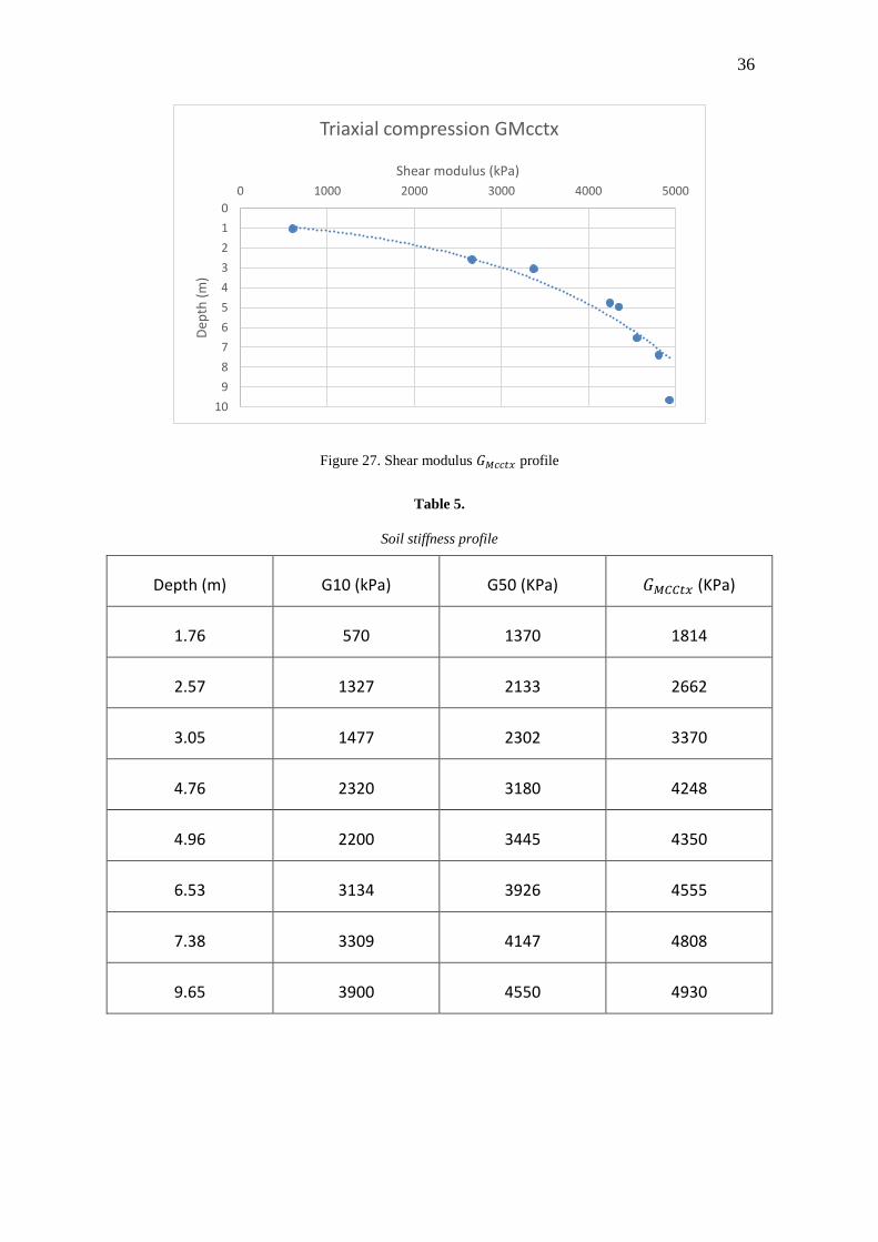
𝐺𝑀𝐶𝐶𝑡𝑥 represents the percentage of the total change in deviatoric stress. Figure 24 shows
the elastic shear modulus from stress- strain graph at depth 4.75 m. By using the stress- strain
theory, three stiffness values for varies depth are plotted. Following the same procedures,
shear modulus at varies depth can be calculated in Table 4. Figure 25, Figure 26 and Figure 27
represents the linear line trend of shear modulus at each point. After that, soil stiffness at
foundation level 1.5 m can be estimated.
Figure 24. Shear modulus profile for TX at depth 4.75m

35
Figure 25. Shear modulus 𝐺10 profile
Figure 26. Shear modulus 𝐺50 profile
0
1
2
3
4
5
6
7
8
9
10
0 500 1000 1500 2000 2500 3000 3500 4000D
epth
(m
)
Shear modulus (kPa)
Triaxial Compression G10
0
1
2
3
4
5
6
7
8
9
10
0 1000 2000 3000 4000 5000
Dep
th (
m)
Shear modulus (kPa)
Triaxial Compression G50
36
Figure 27. Shear modulus 𝐺𝑀𝑐𝑐𝑡𝑥 profile
Table 5.
Soil stiffness profile
Depth (m) G10 (kPa) G50 (KPa) 𝐺𝑀𝐶𝐶𝑡𝑥 (KPa)
1.76 570 1370 1814
2.57 1327 2133 2662
3.05 1477 2302 3370
4.76 2320 3180 4248
4.96 2200 3445 4350
6.53 3134 3926 4555
7.38 3309 4147 4808
9.65 3900 4550 4930
0
1
2
3
4
5
6
7
8
9
10
0 1000 2000 3000 4000 5000D
epth
(m
)
Shear modulus (kPa)
Triaxial compression GMcctx

37
4.2.2 Shear modulus results for SBPM
The shear modulus for SBPM can be determined from the stress-strain curve. Figure 28
represents the cavity pressure versus strain at depth 2.15m, 3.2m and 5.5m. Shear modulus
can be determined by an unload- reload loop carried out at a nominated cavity strain.
G = 1
2 𝑑𝑝
𝑑Ɛ (32)
Where, G = shear modulus, 𝑑𝑝
𝑑Ɛ = the gradient of total pressure to cavity strain
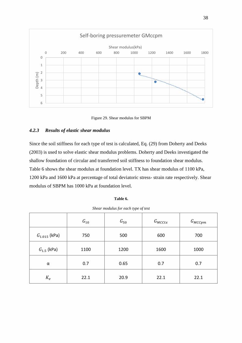
Shear modulus at three depth are 1020 kPa, 1240 kPa, 1480 kPa. A linear trend line can be
created to estimate the shear modulus at foundation level 1.5 m. This is shown in Figure 29.
Figure 28. Pressuremeter data at varies depth
0
0.02
0.04
0.06
0.08
0.1
0.12
0.14
0.16
0.18
0.2
0 0.2 0.4 0.6 0.8 1 1.2
Cvi
ty p
ress
ure
(M
Pa)
Cavity strain (%)
Self-boring Pressuremeter
Data depth 2.15m
Data depth 3.2m
Data depth 5.5m
38
Figure 29. Shear modulus for SBPM
4.2.3 Results of elastic shear modulus
Since the soil stiffness for each type of test is calculated, Eq. (29) from Doherty and Deeks
(2003) is used to solve elastic shear modulus problems. Doherty and Deeks investigated the
shallow foundation of circular and transferred soil stiffness to foundation shear modulus.
Table 6 shows the shear modulus at foundation level. TX has shear modulus of 1100 kPa,
1200 kPa and 1600 kPa at percentage of total deviatoric stress- strain rate respectively. Shear
modulus of SBPM has 1000 kPa at foundation level.
Table 6.
Shear modulus for each type of test
𝐺10 𝐺50 𝐺𝑀𝐶𝐶𝑡𝑥 𝐺𝑀𝐶𝐶𝑝𝑚
𝐺1.015 (kPa) 750 500 600 700
𝐺1.5 (kPa) 1100 1200 1600 1000
α 0.7 0.65 0.7 0.7
𝐾𝑣 22.1 20.9 22.1 22.1
0
1
2
3
4
5
6
0 200 400 600 800 1000 1200 1400 1600 1800
Dep
th (
m)
Shear modulus(kPa)
Self-boring pressuremeter GMccpm

39
4.2.4 Results of foundation settlement
As discussed in section 3.4.1, the efficiency settlements under working loads are estimated to
investigate load- settlement response. For serviceability design, settlements at 25%, 50% of
ultimate failure load (𝑢25, 𝑢50 ) are investigated.
Table 7.
Foundation settlements for TX and SBPM
𝐺10 𝐺50 𝐺𝑀𝐶𝐶𝑡𝑥 𝐺𝑀𝐶𝐶𝑝𝑚
𝐺1.015 (kPa) 750 500 600 700
𝑢25 (mm) 3.04 4.8 3.8 3.3
𝑢50 (mm) 6.1 9.7 7.6 6.5
𝑢100 (mm) 12.2 19.3 15.3 13.1
The load-settlement graphs for each soil stiffness are shown in Figure 30. The blue curve
represents the measured foundation performance for unconsolidated undrained test (UU).
The measured UU test has settlement and ultimate failure load in Table 8. The settlement at
25%, 50% and 100% of failure load is 3mm, 6mm and 22 mm respectively. In Figure 30, it can
be found that the 𝐺10 and 𝐺𝑀𝐶𝐶𝑝𝑚 has a remarkable prediction for 𝑢25 and 𝑢50 compare with
UU tests. The soil stiffness for TX- 𝐺𝑀𝐶𝐶𝑡𝑥 also has a good estimation for 𝑢25 and 𝑢50. While
most of types have different values for ultimate settlement.
Table 8.
Foundation performance for UU test
Measured Values
Failure Load Q (KN) 205
𝑢25 (mm) 3
𝑢50(mm) 6

40
𝑢100(mm) 22
Figure 30. Load settlement for each soil stiffness
4.2.5 Results of FEA
In this section a Tresca soil model was simulated by geotechnical software- Plaxis 2D to
analyse the soil behaviour of foundation in Ballina. The material input data has been discussed
in section 4.5. The crust layer is clayey silty sand with 1.5 m thickness, underlay by 8.5 m
thickness of estuarine clay. The GW is 1 m below the ground surface. This is shown in Figure
31. To consider the horizontal deformation of crust, the axis boundary should be long enough
to avoid unexpected soil collapse. Therefore, 30 m is used for soil layer length.
0
50
100
150
200
250
0 5 10 15 20 25 30 35
Failu
re lo
ad Q
(K
N)
Settlement (mm)
Load settlement graph for each soil stiffness
G10
G50
Gmcctx
GMccpm
UU2

41
Figure 31. Plan view of FEA model
The model set the dimensions of square foundation and excavation pit as circle. Therefore,
the foundation and excavation pit have radius of 1.013 m and 1.315 m. The simulation stage
consists of two steps, which include excavates a 1.315m width and 1.5 m depth pit, creates a
in situ footing with cumulative load until failure. In reality, each concrete block has a weight
about 3.3 tonnes with a unit weight of 24 KN/𝑚2, which represents that each block increases
the pressure about 10 kPa. Figure 34 shows the finite element mesh once the geometry setting
is completed. Figure 33 shows the failure mechanism of FEA. It can be found that the failure
happened surrounding by footings and the horizontal deformation can be neglected. The
failure mechanism indicates that the clayey silty sand forced the deformation happened in the
gap between footing and excavation wall. The crust is strong enough to make this
phenomenon occur.
Figure 34 shows the load settlement response of model compare with the UU test. It can be
found that FEA model provides a reasonable fit to the measured values performance. The
settlement values of 𝑢25 and 𝑢50 are close for both curves.
Figure 32. Mesh generating for FEA model

42
Figure 33. Total deformation of foundation
Figure 34. FEA load-settlement graph
0
50
100
150
200
250
0 10 20 30 40 50
Failu
re lo
ad Q
(K
N)
Settlement (mm)
Load- settlement graph
UU test
FEA
43
5 ANALYSIS AND DISCUSSION
5.1 UNDRAINED SHEAR STRENGTH AND SETTLEMENT
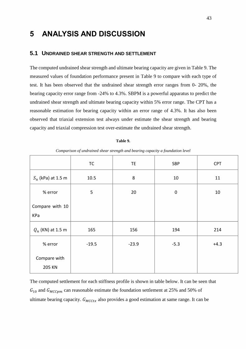
The computed undrained shear strength and ultimate bearing capacity are given in Table 9. The
measured values of foundation performance present in Table 9 to compare with each type of
test. It has been observed that the undrained shear strength error ranges from 0- 20%, the
bearing capacity error range from -24% to 4.3%. SBPM is a powerful apparatus to predict the
undrained shear strength and ultimate bearing capacity within 5% error range. The CPT has a
reasonable estimation for bearing capacity within an error range of 4.3%. It has also been
observed that triaxial extension test always under estimate the shear strength and bearing
capacity and triaxial compression test over-estimate the undrained shear strength.
Table 9.
Comparison of undrained shear strength and bearing capacity a foundation level
TC TE SBP CPT
𝑆𝑢 (kPa) at 1.5 m 10.5 8 10 11
% error
Compare with 10
KPa
5 20 0 10
𝑄𝑢 (KN) at 1.5 m 165 156 194 214
% error
Compare with
205 KN
-19.5 -23.9 -5.3 +4.3
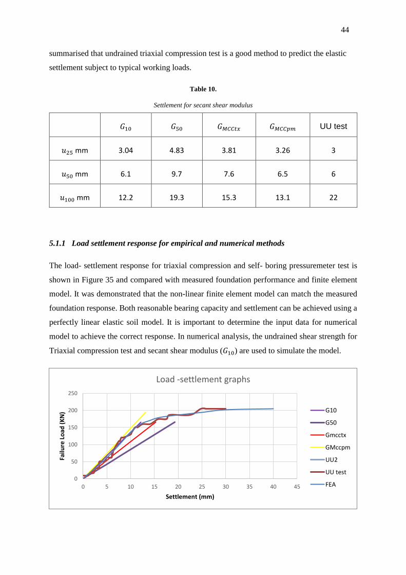
The computed settlement for each stiffness profile is shown in table below. It can be seen that
𝐺10 and 𝐺𝑀𝐶𝐶𝑝𝑚 can reasonable estimate the foundation settlement at 25% and 50% of
ultimate bearing capacity. 𝐺𝑀𝐶𝐶𝑡𝑥 also provides a good estimation at same range. It can be
44
summarised that undrained triaxial compression test is a good method to predict the elastic
settlement subject to typical working loads.
Table 10.
Settlement for secant shear modulus
𝐺10 𝐺50 𝐺𝑀𝐶𝐶𝑡𝑥 𝐺𝑀𝐶𝐶𝑝𝑚 UU test
𝑢25 mm 3.04 4.83 3.81 3.26 3
𝑢50 mm 6.1 9.7 7.6 6.5 6
𝑢100 mm 12.2 19.3 15.3 13.1 22
5.1.1 Load settlement response for empirical and numerical methods
The load- settlement response for triaxial compression and self- boring pressuremeter test is
shown in Figure 35 and compared with measured foundation performance and finite element
model. It was demonstrated that the non-linear finite element model can match the measured
foundation response. Both reasonable bearing capacity and settlement can be achieved using a
perfectly linear elastic soil model. It is important to determine the input data for numerical
model to achieve the correct response. In numerical analysis, the undrained shear strength for
Triaxial compression test and secant shear modulus (𝐺10) are used to simulate the model.
0
50
100
150
200
250
0 5 10 15 20 25 30 35 40 45
Failu
re L
oad
(K
N)
Settlement (mm)
Load -settlement graphs
G10
G50
Gmcctx
GMccpm
UU2
UU test
FEA

45
Figure 35. Load- settlement graph for hand calculation and numerical analysis
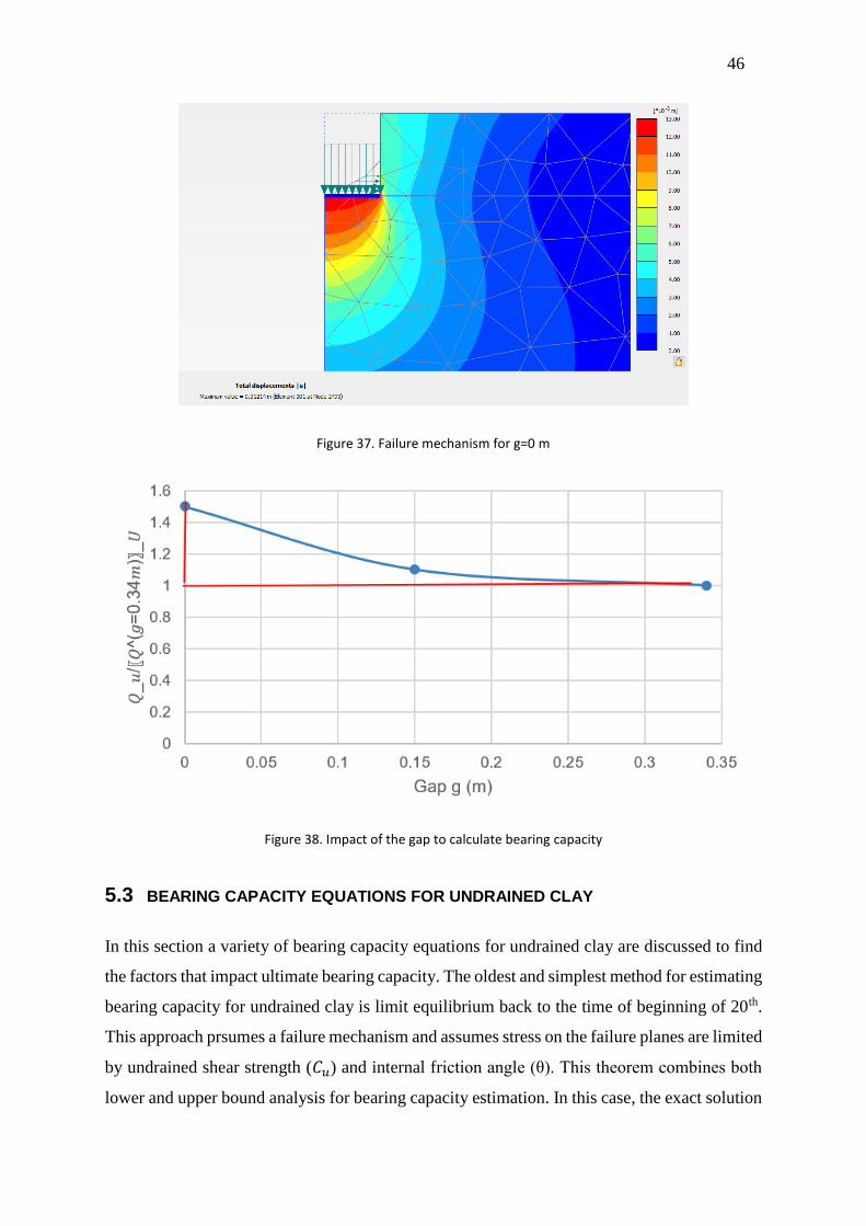
5.2 BOUNDARIES IMPACT FOR NUMERICAL ANALYSIS
In this section, the effect of gap between foundation and excavation wall will be investigated.
In Fig 36, the failure condition occurred around footings, extending only to the edge of
excavation wall. The gap between footings and excavation wall can significantly impact the
load settlement response for FEA analysis. Fig 37 shows the foundation embedded with no
gap. It was found that the impact of deformation extends to the edge and part of stress loads on
the excavation wall. The total settlement reduces from 22 mm to 12 mm and ultimate failure
load increase up to 50% compared with original model. A non-linear graph in Fig 38 shows
the impact of the gap between footing and stand wall. The Y-axis represents the rate of ultimate
failure load. It was found that the increase of gap would over-predict foundation’s ultimate
bearing capacity.
Figure 36. Failure mechanism for g=0.34 m
46
Figure 37. Failure mechanism for g=0 m
Figure 38. Impact of the gap to calculate bearing capacity
5.3 BEARING CAPACITY EQUATIONS FOR UNDRAINED CLAY
In this section a variety of bearing capacity equations for undrained clay are discussed to find
the factors that impact ultimate bearing capacity. The oldest and simplest method for estimating
bearing capacity for undrained clay is limit equilibrium back to the time of beginning of 20th.
This approach prsumes a failure mechanism and assumes stress on the failure planes are limited
by undrained shear strength (𝐶𝑢) and internal friction angle (θ). This theorem combines both
lower and upper bound analysis for bearing capacity estimation. In this case, the exact solution

47
for limit equilibrium is derived from 4𝐶𝑢≤ q ≤ 5.52𝐶𝑢 and is given by Prandtl (1921) as q =
(2+π) 𝐶𝑢 = 5.14𝐶𝑢
Table 11.
Prandtl’s equation data
Prandtl’s estimation of bearing capacity
Q= 5.14𝐶𝑢
Undrained shear strength
𝑐𝑢 (KPa)
Ultimate bearing
capacity (KPa)
Failure Load
(KN)
10 51.4 166
The measured failure load is 166 kN, which is 19% less than the expect failure load 205 kN.
This method has disadvantage of considering shape factors. It is necessary to guess the shape
of foundations and poor guess giving wrong estimation of bearing capacity.
In literature review, it has been discussed that Terzaghi (1943) was the first person to develop
a comprehensive bearing capacity theory for shallow foundation. Based on the load failure
mechanism shown in Fig 39, he developed equations of estimating bearing capacity of shallow
foundations. The equation depends on the shape of foundations, which is shown in below
𝑞𝑢𝑙𝑡 = 1.3𝑐′𝑁𝑐 + q𝑁𝑞 + 0.4YB𝑁𝑦
Where, 𝑁𝑐, 𝑁𝑞, 𝑁𝑦 is dimensionless bearing capacity factor, 𝑐′ is effective cohesion, q is
surcharge at the ground surface.
In Ballina case, the undrained shear strength 𝑠𝑢 at foundation level is given as 10 kPa, with 0°
of friction angle and unit weight of sand 17 KN/𝑚2. By selecting Terzaghi’s bearing capacity
factor, the ultimate failure load is given as 332 KN, which is shown in Table 11.
Table 12.
Terzaghi’s equation data
Terzaghi’s bearing capacity factor Effective stress/ Surcharge Ultimate bearing
capacity
Ultimate load
failure
𝑁𝑐 𝑁𝑞 𝑁𝑦 q = YD (KN) 𝑞𝑢𝑙𝑡 (KPa) Q (KN)

48
5.7 1 0 25.5 99.6 332
Figure 39. Terzaghi’s bearing capacity factor (Geotechnical Engineering Design, 2015)
Skempton (1951) developed a simple equation to estimate the ultimate bearing capacity with
factor 𝑁𝑐 and undrained shear strength under undrained conditions. In literature review, it has
been discussed that Susan, et al (2006) investigated the undrained bearing capacity of square
footings and modified Skmpton’s prediction of 𝑁𝑐 to 5.9 for a rough square footing.
𝑞𝑢𝑙𝑡 = 𝑐𝑢𝑁𝑐
Table 13.
Terzaghi’s equation data
Terzaghi’s bearing capacity factor Undrained cohesion Ultimate bearing
capacity
Ultimate load
failure
𝑁𝑐 𝑐𝑢 (KPa) 𝑞𝑢𝑙𝑡 (KPa) Q (KN)

49
5.9 10 59 191.2
In both equations, it can be found bearing capacity factors have a significantly influence to
estimate the ultimate failure load. The empirical factors mainly depends on the internal
friction angle, interaction between foundation and soil and shape of foundations. Many
investigators modified bearing capacity factors in different methods and it is necessary to
take all foundation design elements into account to get the reasonable results.
50
6 CONCLUSIONS
Bearing capacity plays an important role for foundation design and perhaps the most important
part for soil engineering. Failing to recognise the bearing capacity can cause foundation failures
and the entire building project becomes unsafe. In the past, the investigation of large-scale
shallow foundation tests on soft clay is lmited. Most of data comes from UK’s national soft
soil test site, Bothkennar, Scotland. Australian National Field - Testing Facility was built in
Ballina, NSW in 2013. The site investigation was conducted in this area and a series of in situ
and laboratory tests were investigated.
The aim of this project was to investigate the bearing capacity behaviour of foundations
especially for undrained bearing capacity of square footings on soft clays. With the literature
review of fundamental knowledge of bearing capacity, it was found that Terzaghi’s (1943)
bearing capacity theory is most widely used one to estimate bearing capacity of shallow
foundations. While Terzaghi’s bearing capacity did not take the effects of footer depth, load
inclination factor, soil compressibility, and water tables. Skempton (1951) reconsidered
Terzaghi’s equation and found bearing capacity factor 𝑁𝑐 increase with foundation depth. The
bearing capacity factor and shape factor he obtained was 𝑁𝑐 = 6.17 and 𝑆𝑐 = 1.2 for rough
square footings. The other few studies such as Salgado (2004), Susan (2006) investigated the
bearing capacity behaviour of square footings and proposed that 𝑁𝑐 = 5.52, 𝑆𝑐 = 1.1, 𝑁𝑐 = 5.9,
𝑆𝑐 = 1.15 respectively.
In Ballina case, the undrained shear strength relationship with its foundation relationship was
investigated. The results obtained from modified Terzaghi’s equation demonstrated that the
undrained shear strength has a direct proportional relationship with ultimate bearing capacity.
𝑄𝑢 = 19.44 𝑆𝑢. The results calculated from in situ tests- CPT and SBM indicate that both tests
have reasonable estimation for ultimate bearing capacity within an error range of 5 %. While
the laboratory tests- TC & TE can’t predict the ultimate bearing capacity precisely. It has also
been observed the TE test under estimate undrained shear strength around 20% and ultimate
bearing capacity around 24%. For serviceability limit design, the effective settlements under
working load is used to predict the foundation behavior. It was found that the secant shear
modulus 𝐺10 and 𝐺𝑀𝐶𝐶𝑝𝑚 can provide a good estimation of vertical settlement, while 𝐺𝑀𝐶𝐶𝑡𝑥
also has a reasonable estimation.

51
In FEA analysis, a linear elastic Tresca soil model is adopted and applied using given data. The
input data includes the previous test calculation such as undrained shear strength (10 kPa),
Poisson’s ratio (0.495), Young’s modulus (3MPa), groundwater table (0.5m AHD), material
unit weight etc. The load- settlement response of measured foundation performance from (UU)
test was proved to be well predicted by numerical model. Through the output of deformation
graph, it was observed that the gap between footing and excavation wall has a significant
impact to the ultimate bearing capacity and vertical settlement. A non- liner curve demonstrated
that the ultimate bearing capacity increase with decrease of gap between footing and slope.
52
9 REFERENCE
Abyaneh, SD, Ojo, A, Maconochie, A, Haghighi, A 2015, ‘The undrained bearing capacity of
shallow foundations subjected to three- dimensional loading Incuding Torison’, The
twenty- fifth International Ocean and Polar Engineering, pp 1-7.
Benmebarek, S, Saifi, I, Benmebarek, N 2017, ‘Depth factors for undrained bearing capacity
of circular footing by numercal approach’, Journal of rock mechanics and
Geotechnical Engineering, vol.9, pp 761-764.
Catanzariti, F 2016, ‘Bearing capacity of shallow foundations’, Geostru, p.11.
Du,p,Liu, XL & Zhang, YF 2017, ‘ Disscussion of the Method to Determine the Ultimate
Bearing Capacity of Soil Foundation’, IOP Conference: Earth and Environmental
Science, pp 1-4.
Doherty, J.P, Gourvenec, S, Gaone, F.M 2017, ‘Insights from a shallow foundation load-
settlement prediction exercise’, Computers and Geotechnics, Vol.93, pp 269-279.
Gui, D 1995, ‘Bearing capacity of shallow foundation on simulated lunar soil’, Master thesis,
Montana State University, USA.
Gourvenec, S, Randolph, M& Kingsnorth, O 2006, ‘Undrained bearing capacity of square and
rectangular footings’, International Journal of Geotechnicals, pp. 146-155.
Gagone, F.M, Gourvenec, S, Doherty, J.P 2018, ‘Large- scale shallow foundation load tests on
soft clay- At the National Filed Testing Facility (NFTF), Ballina, NSW, Australia’,
Computers and Geotechnics, Vol. 93, pp 253-268.
Hansen, J.B 1970,’ A revised and extended formula for bearing capacity’, Geoteknisk Institut,
pp 4-10.
Hartsfiled, RJ 2013,’ ‘Upper bound analysis of bearing capacity and overturing capacities of
shallow foundation in soft clay’, Master thesis, Texas A&M University, USA.
Lianapathirana, D.S, Carter, J.P 2005, ‘Undrained bearing capacity of Shallow foundations on
structured soils’, Proceedings of the International Symposium on Frontiers in Offshore
Geotechnics, Western Sydney University, Sydney, pp 2-4.
Michalowski, R.I 2001, ‘Upper-bound load estimates on square and rectangular footings’,
Geotechnique 51, No.9, pp 787-798.

53
Mohamed, FMO 2014, ‘Bearing capacity and settlement behaviour of footings subjected to
static and seismic loading conditions in unsaturated sandy soils’, Phd thesis, University
of Ottawa, Canada.
Remai, Z 2012, ‘Correlation of undrained shear strength and CPT resistance’, Budapest
University of Technology and Economics, pp 39-41.
Salagado, R, Lyamin, A.V, Sloan, S.W& Yu, H.S 2006, ‘Two and three- dimensional bearing
capacity of foundations in clay’, Geotechnique 54, No.5, pp 297-306.
Sitharam, TG 2013,’ Advanced Foundation Engineering’, Shallow foundations, Indian
Institute of Science, Bangalore.
Strahler, AW 2012, ‘Bearing Capacity of Immediate Settlement of Shallow Foundations on
clay’, Master thesis, Oregon State University, USA.
Quadir, MA 1990, ‘Bearing Capacity of Strip Footing on Sand’, Master thesis, Bangladesh
University, Dhaka.
Quoc, V.N 2008, ‘Numerical modelling of the undrained vertical bearing capacity of shallow
foundations’, Master thesis, University of Southern Queensland, Queensland.
Xiao, M 2015, ‘Geotechnical Engineering Design’, The Pennsylavania State University, pp
10-16.