Beams on Elastic Foundation - University of British...

Professor Terje Haukaas University of British Columbia, Vancouver www.inrisk.ubc.ca

Beams on Elastic Foundation Updated March 10, 2014

Beams on Elastic Foundation Beams on elastic foundation, such as that in Figure 1, appear in building foundations, floating structures, beams that rest on a grid of perpendicular beams, and elsewhere. It also turns out that the governing differential equation is similar to that of cylindrical shells and tapered beams with curved webs. As a result, this material has quite broad applicability. However, it is important to exercise caution when applying this theory to problems where the foundation does not behave in a linear fashion, such as soils that respond nonlinearly to pressure or ships whose waterline area changes with sinkage. In this document the beam is assumed to be an ordinary Euler-Bernoulli beam, thus the theory from that document carries over to this one. Accordingly, downwards distributed load on the beam is referred to as q, while it is denoted qz when it acts in the opposite direction, i.e., in the z-direction.

Figure 1: Beam on elastic foundation.

Foundation Stiffness The foundation stiffness, ks, which is illustrated in Figure 1, is conceptually straightforward. When the beam displaces downwards, the foundation exerts an upwards force, illustrated by the springs in Figure 1. ks has units of force per unit length along the beam. Another stiffness, denoted kφ, is also present, relating to rotation φ of the beam cross-section around the longitudinal axis of the beam. In other words, kφ provides resistance against torsion of the beam. Techniques to determine ks and kφ are described in the following subsections for different situations.

Stiffness from Buoyancy An important application of this theory is floating structures. To determine ks for a beam that floats in water, suppose the beam cross-section has width equal to b at the location where the cross-section penetrates the water surface. Furthermore, let the mass density of water be denoted ρw, which typically equals 1,025kg/m3 for seawater, and let g denoted the acceleration of gravity. For an infinitesimal beam length, dx, the change in buoyancy force due to a vertical displacement Δ equals the weight of the displaced water, namely weight density multiplied by volume:

B = ρw ⋅ g( ) ⋅ b ⋅dx ⋅ Δ( ) (1)

As a result, the stiffness that resists the displacement Δ, per unit length of the beam, is obtained by dividing B by dx and Δ:

q

ks

P



ks = ρw ⋅ g ⋅b

kNm2

⎡

⎣⎢

⎤

⎦⎥ (2)

which has unit force per unit length squared. The evaluation of ks according to Eq. (2) is correct as long as the beam width at the waterline does not change. Unfortunately, this condition is not always satisfied, which is understood from Figure 2. While the rectangular beam-cross-section maintains width b regardless of the vertical displacement, the value of b for the circular cross-section varies with the heave motion. As a result, ks is a function of Δ for the circular cross-section, which introduces nonlinearity that is neglected in the subsequent equations.

Figure 2: Heave and roll motion of floating beams.

The fact that the waterline area is only a proxy for displaced water volume becomes even more apparent when determining kφ. To understand this, first consider the classical approach for determining kφ. When the rectangular beam-cross-section in Figure 2 rotates counterclockwise as indicated by dashed lines, more water is displaced on the left side and less water is displaced on the right side. As a result, buoyancy forces act against the rotation, giving rise to kφ. By computing the volumes of the shaded triangles in Figure 2 the resultant buoyancy force, on either side, is

R = ρw ⋅ g( ) ⋅ 1

2⋅ b2⋅ b2⋅φ ⋅dx (3)

The distance between the force pair, i.e., the buoyancy forces from each of the shaded triangles in Figure 2 is 2/3 of b. Thus, the moment from buoyancy that resists the rotation is

T = R ⋅ 2

3⋅b = ρw ⋅ g ⋅

b3

12⋅φ ⋅dx (4)

As a result, the stiffness that resists the rotation φ, per unit length of the beam, is obtained by dividing T by dx and φ:

kφ = ρw ⋅ g ⋅

b3

12 (5)

where it is observed that the moment of inertia of the waterline area. Again it is observed that the derivations do not hold for the circular cross-section in Figure 2. In fact, it is

b b

ϕ



easily seen that cross-section has zero resistance against rotation. If not easily seen, it is easily felt when trying to balance on a floating timber log. The problem with applying Eq. (5) to the circular cross-section is the use of movement of the beam at the waterline as a proxy for displaced water volume. Thus, while Eq. (5) is commonly used, it is important to be aware of its limitations.

Stiffness from Soil Suppose the stiffness, ks, is determined from soil testing. In particular, suppose a vertical load, P, is placed on an area with dimensions x and y, and that the vertical displacement, Δ, is measured. The relationship between the distributed load and the displacement is written in terms of a distributed stiffness, kd:

Px ⋅ y

= kd ⋅ Δ ⇒ kd =P

Δ ⋅ x ⋅ yNm3

⎡

⎣⎢

⎤

⎦⎥ (6)

While kd is stiffness per unit area, ks is stiffness per unit length. The sought value is obtained by multiplying kd by the beam width, b:

ks = b ⋅ kd

Nm2

⎡

⎣⎢

⎤

⎦⎥ (7)

If one assumes that the foundation material is linear elastic, there is no unique relationship between the Young’s modulus, E, of the foundation material and the stiffness ks. However, if one imagines that the soil underneath the beam is linear elastic with depth L to bedrock then the force-deformation relationship of the soil is

P = EA

L⋅ Δ (8)

where A=x.y is the area loaded by P. Writing Eq. (8) in the form of Eq. (6) yields

Px ⋅ y

= kd ⋅ Δ ⇒ kd =EL

Nm3

⎡

⎣⎢

⎤

⎦⎥ (9)

and the sought stiffness is, in accordance with Eq. (7):

ks = b ⋅ kd =

b ⋅EL

Nm2

⎡

⎣⎢

⎤

⎦⎥ (10)

Stiffness from Girder Grid Another situation appears when the beam is resting on a grid of closely spaced perpendicular beams, e.g. joists. Suppose the joists are spaced at x on centre and that their stiffness against vertical deflection at the point of intersection with the beam is kb[N/m]. Then the sought stiffness is:

ks =

kb

xNm2

⎡

⎣⎢

⎤

⎦⎥ (11)



Bending Differential Equation Compared with the basic Euler-Bernoulli beam theory, it is sufficient to modify the equation for vertical equilibrium to obtain the differential equation for a beam on elastic foundation. As a result, the following conventions from basic beam bending hold valid: 1) Clockwise shear force is positive; 2) Bending moment with tension at the bottom is positive; 3) Tension stress is positive; 4) The z-axis points upwards, so that upwards displacement, w, is positive; 5) The distributed load, qz, is positive upwards. Figure 3 shows the forces acting on an infinitesimal beam element. The springs that illustrate the elastic foundation exert a downward force when the beam is subjected to an upward displacement.

Figure 3: Infinitesimal beam element.

Vertical equilibrium yields:

qz ⋅dx − ks ⋅w ⋅dx − dV = 0 (12)

Dividing by dx and re-arranging yields

qz =

dVdx

+ ks ⋅w (13)

Substitution of this equation into the Euler-Bernoulli beam theory yields the following revised differential equation

EI ⋅ d

4wdx4

+ ks ⋅w = qz (14)

Another way of deriving the differential equation is to start with the following basic differential equation for beam bending:

EI ⋅ d

4wdx4

= qz (15)

dx

V M M+dM V+dV

ks

x

z, w

qz



From earlier it is understood that the applied load, qz, plus the elastic foundation yields a total force on the beam element equal to qz–ksw. By substituting this total load in the right-hand side of Eq. (15), Eq. (14) is obtained. For convenience, it is rewritten on the form

d 4wdx4

+ ksEI

⋅w =qzEI

(16)

In solving this differential equation it is useful to define a “characteristic length,” sometimes referred to as the elastic length. To approach the definition it is first noted that EI/ks has dimension [m4]. As a result, the following definition of the characteristic length has the dimension of length:

lc ≡

4 ⋅EIks

4 ⇒ EIks

= lc4

4 (17)

The convenience of the factor 4 will become apparent later. It is also convenient to work with the normalized coordinate ξ instead of the original coordinate, x, along the beam:

ξ = x

lc (18)

To transform the differential equation, differentiation with respect to x is related to differentiation with respect to ξ by the chain rule of differentiation:

ddx

= ddξ

⋅ dξdx

= 1lc⋅ ddξ

(19)

Hence, the fourth-order derivative with respect to x equals the fourth-order derivative with respect to ξ divided by lc4, which yields the following homogeneous version of the transformed differential equation, now formulated in the coordinate ξ:

d 4wdξ 4

+ 4 ⋅w = 0 (20)

General Solution The characteristic equation is γ4+4=0 has the four different complex roots (1+i), (1–i), (–1+i), and (–1–i). Consequently, the general solution is:

w(ξ ) = C1 ⋅e−ξ cos(ξ )+C2 ⋅e

−ξ sin(ξ )"Damped terms"

+C3 ⋅e

ξ cos(ξ )+C4 ⋅eξ sin(ξ )

"Undamped terms"

(21)

where the phrase “damped terms” is employed to identify terms that vanish as ξ increases to infinity. This labeling is useful because the solution for a point load must vanish far away from the point of load application. In fact, only the damped terms appear in many practical situations. To shorten the notation under such circumstances, the following auxiliary functions are defined:

g1 = e−ξ cos(ξ ) (22)



g2 = e−ξ sin(ξ ) (23)

g3 = g1 + g2 (24)

g4 = g1 − g2 (25)

These functions are plotted in Figure 4, where it is observed that they decay rapidly with ξ. In fact, all functions approach zero once ξ increases beyond 4.

Figure 4: g-functions.

The auxiliary functions also have the following properties:

dg1

dξ= −g3

dg2

dξ= g4

dg3

dξ= −2g2

dg4

dξ= −2g1 (26)

These relationships are helpful for deriving the bending moment, etc. from the general solution. The starting point is the general solution with only the damped terms, which reads:

w(ξ ) = C1 ⋅ g1 +C2 ⋅ g2 (27)

Differentiation yields the rotation:

θ(ξ ) = dw

dx= 1

lc

⋅ dwdξ

= − 1lc

⋅ C1 ⋅ g3 −C2 ⋅ g4( ) (28)

Another differentiation yields the bending moment:

M = EI ⋅ d 2w

dx2 = EI ⋅ dθdx

= EI ⋅ 1lc

⋅ dθdξ

= 2EIlc

2 ⋅ C1 ⋅ g2 −C2 ⋅ g1( ) (29)

1 2 3 4 5 6x

0.20.40.60.81.0g1

1 2 3 4 5 6x

0.050.100.150.200.250.30

g2

1 2 3 4 5 6x

0.20.40.60.81.0g3

1 2 3 4 5 6x

-0.2

0.20.40.60.81.0g4



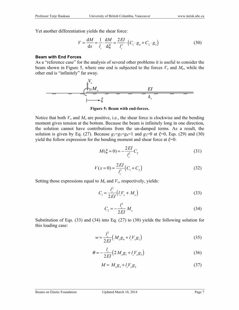
Yet another differentiation yields the shear force:

V = dM

dx= 1

lc

⋅ dMdξ

= 2EIlc

3 ⋅ C1 ⋅ g4 +C2 ⋅ g3( ) (30)

Beam with End Forces As a “reference case” for the analysis of several other problems it is useful to consider the beam shown in Figure 5, where one end is subjected to the forces Vo and Mo, while the other end is “infinitely” far away.

Figure 5: Beam with end-forces.

Notice that both Vo and Mo are positive, i.e., the shear force is clockwise and the bending moment gives tension at the bottom. Because the beam is infinitely long in one direction, the solution cannot have contributions from the un-damped terms. As a result, the solution is given by Eq. (27). Because g1=g3=g4=1 and g2=0 at ξ=0, Eqs. (29) and (30) yield the follow expression for the bending moment and shear force at ξ=0:

M (ξ = 0) = − 2EI

lc2 C2 (31)

V (x = 0) = 2EI

lc3 C1 +C2( ) (32)

Setting those expressions equal to Mo and Vo, respectively, yields:

C1 =

lc2

2EIlcVo + Mo( ) (33)

C2 = −

lc2

2EIMo (34)

Substitution of Eqs. (33) and (34) into Eq. (27) to (30) yields the following solution for this loading case:

w =

lc2

2EIMog4 + lcVog1( ) (35)

θ = −

lc

2EI2Mog1 + lcVog3( ) (36)

M = Mog3 + lcVog2 (37)

!

Mo

VoEIks



V = − 2

lc

Mog2 +Vog4 (38)

Beam with Point Load The previous solution is now utilized to analyze the infinitely long beam in Figure 6, which has a point load applied at ξ=0.

Figure 6: Beam with point load.

Immediately to the left of the point load the shear force is P/2, while immediately to the right it is –P/2. That is, with reference to the previous case, Vo=–P/2. Furthermore, the rotation at the point load is zero:

θ(0) =

lc

2EI2Mo + lcVo( ) = 0 (39)

Substituting Vo=–P/2 and solving for Mo yields

Mo =

P ⋅ lc

4 (40)

where it is noted that the bending moment at the point load is the same as that of a simply supported beam with length lc loaded at midspan. In fact, that is the reason that the integer 4 was introduced in the definition of lc in Eq. (17). In short, the solution for the beam in Figure 6 is given by Eqs. (35) to (38) with

Vo = − P

2 (41)

and

Mo =

lc P4

(42)

That yields the following solution for a beam on an elastic foundation with a point load:

w =

Plc3

8EIg4 − 2g1( ) (43)

θ = −

Plc2

4EIg1 − g3( ) (44)

M =

Plc

4g3 − 2g2( ) (45)

!

EIks

P



V = − P

2⋅ g2 + g4( ) (46)

This solution, as the previous ones, is defined only for positive ξ-values. However, it is readily plotted on both sides of the origin by multiplying Eqs. (44) and (46) by the sign of ξ, namely ξ/|ξ|. This is done because the rotation and the shear force are asymmetric functions. For example, from the discussion before Eq. (39) it is clear that the shear force is positive where ξ is negative, and vice versa. Another common plotting convention is to multiply Eq. (45) by (–1) to get the moment diagram on the tension side of the beam.

Cluster of Point Loads If more than one point load is present, such as the situation in Figure 7, the solution is obtained by superposition. Assuming that the beam is sufficiently long for the solution to “dampen out” before the beam end is reached, the solution in Eqs. (43) to (46) is employed. For example, for the situation in Figure 7 the bending moment is:

M =

P0 ⋅ lc

4g3(ξ )− 2g2(ξ )( ) + Pi ⋅ lc

4g3(ξ −ξi )− 2g2(ξ −ξi )( )

i=1

2

∑ (47)

Figure 7: Beam with point load cluster.

Distributed Load Above, the solutions w, θ, M, and V were established for a beam with a point load. That solution can also be employed in the analysis of beams with distributed load. The point load that was previously applied at ξ=0 is now applied at the generic location ξ=c. Moreover, the point load, P, is considered to be one infinitesimal part of a distributed load, i.e., P=q.dx. Because dx=lc.dξ the load to be inserted into the previous solutions w(ξ), θ(ξ), M(ξ), and V(ξ) is P=q.lc.dξ. On that basis, the solution for a distributed load between ξ=a and ξ=b is

w(ξ ) = w(ξ − c)dc

a

b

∫ = −qlc

3

8EI⋅ lc ⋅ g4(ξ − c)− 2g1(ξ − c)( )dc

a

b

∫ (48)

etc. for the θ(ξ), M(ξ), and V(ξ), assuming constant load intensity, q.

ξ

EIks

P0 P1 P2

ξ1

ξ2



Torsion Differential Equation The differential equation for St. Venant torsion, without resistance from an elastic foundation, is GJ ⋅φ ''+mx = 0 (49)

The torsional resistance from an elastic foundation is a distributed torque equal to kφ.φ, which implies that the effective distributed torque is equal to mx–kφ.φ. That leads to the following modified differential equation for St. Venant torsion:

φ ''−kφGJ

⋅φ + mx

GJ= 0 (50)

Now consider the homogeneous version of this equation, i.e., let mx=0, and define the auxiliary quantity

lc =GJkφ

(51)

which is the characteristic length in torsion. This definition gives a length-measure because kφ is in units of force. As done previously for bending, the normalized coordinate ξ is defined as in Eq. (18): ξ=x/lc, with resulting differentials given in Eq. (19). This means that the homogeneous version of Eq. (50) is

d 2φdx2

− 1lc2 ⋅φ = 1

lc2 ⋅d 2φdξ 2

− 1lc2 ⋅φ = d 2φ

dξ 2−φ = 0 (52)

General Solution The characteristic equation is γ2+γ=0 has the two roots γ=0 and γ=1. Consequently, the general solution is:

φ = C1 ⋅eξ +C2 ⋅e

−ξ (53)

The torque associated with this solution is

T = GJ ⋅ dφ

dx= GJ ⋅ 1

lc

⋅ C1 ⋅eξ +C2 ⋅e

−ξ( ) (54)

Beam with End Torque As a reference case for the analysis of other problems, consider a beam like the one in Figure 5, with a torque, To, applied at the free end. Because the beam is infinitely long in one direction, the solution cannot have contributions from the “un-damped” term. As a result, C1=0, and the equation that determines C2 is:

To = T (ξ = 0) = GJ ⋅ 1

lc

⋅C2 (55)

which yields



C2 =

To ⋅ lc

GJ (56)

which in turn means that the solution is

φ =

To ⋅ lc

GJ⋅e−ξ (57)

Rigid Beam For cases with long characteristic length relative to the beam length, L, it may be appropriate to consider the beam as a rigid body as it rotates under applied torque, To. In that case the rotation is simply the constant

φo =

To

kφ ⋅ L (58)

and the torque in the beam increases linearly from zero at the free end to

T (x) = kφ ⋅φo ⋅ x = To ⋅

xL

(59)

at a distance x from the free end.

Beams on Elastic Foundation - University of British...

Documents

Transcript of Beams on Elastic Foundation - University of British...