BBD: A NEW BAYESIAN BI-CLUSTERING DENOISING ALGORITHM FOR IASI-NGHYPERSPECTRAL IMAGES

M. Colom1, G. Blanchet2, A. Klonecki3, O. Lezeaux3, E. Pequignot2, F. Poustomis3, C. Thiebaut2, S. Ythier3, J.-M. Morel1

1 CMLA, ENS Cachan. CNRS, Universite Paris-Saclay. 94235, Cachan, France.2 Centre National d’Etudes Spatiales, Toulouse, France.

3 NOVELTIS, 153 rue du Lac, 31670 Labege, France.

ABSTRACT

We propose a new denoising method for 3D hyperspectralimages for the future MetOp-Second Generation series satel-lite incorporating the new IASI-NG interferometer, to belaunched in 2021. This adaptive method retrieves the datamodel directly from the input noisy granule, using the fol-lowing techniques: dual clustering (spectral and spatial),dimensionality reduction by adaptive PCA, and Bayesian de-noising. The use of dimensionality reduction by PCA hasbeen already proven an effective denoising technique becauseof intrinsic data redundancy. We demonstrate here that bycombining a local PCA dimensionality reduction with a dualclustering and a Bayesian denoising, it is possible to improvesignificantly the PSNR with respect to PCA reduction alone.This noise reduction hints at the possibility to multiply ofthe resolution of the satellite by factor 4, while keeping anacceptable SNR .

Index Terms— IASI-NG, denoising, clustering, Bayesian,PCA

1. INTRODUCTION

In 2021 EUMETSAT will launch the first MetOp-SG satel-lite carrying a new interferometer (IASI-NG) developed byCNES1 to measure weather variables, pollution and climatemonitoring, and determining atmospheric gas composition(including H2O,CO2, O3, N2O,CO,CH4) [1, 2]. The in-terferometer is made of 4 captors (one 4×4 PC MCT detectorfor band B1, and MOVPE PV detectors for B2, B3 and B4)which provide 16923 spectral channels between 15.5 and 3.63µm with a spectral resolution of 0.125 cm−1, and a FOV of4×4 pixels for a box of 100×100 km2 at nadir [3]. The noiselevel arriving to the captors is very low with respect to thesignal and in general for HS sounding applications losslesscompression is preferred to avoid damaging the data [4].

Our goal is to denoise 3D hyperspectral IASI-NG images(also called granules) taking advantage of the large redun-dancy of the data. A good enough denoising performance

1The French aerospace agency.

would simply permit to increase the satellite resolution. As arule of thumb, dividing the noise by a factor p would permitto increase the resolution by the same factor. Denoising of HSgranules by using PCA and dimensionality reduction has beenalready explored [5, 6, 7, 8], as well as the problem of group-ing similar signals according to their wavenumber [9]. Herewe propose a Bayesian method to denoise IASI-NG granulescombining dual (spectral and spatial) clustering, a dimension-ality reduction, and an optimal Bayesian method. We call thismethod BBD.

2. THE NOISE MODEL

The IASI-NG instrument is made of four different HS cap-tors with spectral overlapping of ±40 cm−1, each of them af-fected by additive Gaussian noise which depends on both thewavenumber and the intensity (photonic noise). We take intoaccount the IASI-NG worst case for the photonic noise, andtherefore our noise model only depends on the wavenumber(detector noise relying on the focal plane temperature, read-out, and constant ADC noise).

Thus, it is possible to characterize the noise model as afunction which gives the standard deviation of the Gaussiannoise according to the wavenumber. Fig. 1 shows such a noiselevel function. Its peaks are caused by the performance decayat the extremity of bands. The amplitude of the signal is morethan 4700 times higher than the noise.

3. IASI-NG SIMULATED NOISY DATA

The IASI-NG instrument is planned to be launched in 2021and therefore there are no real granule data available. How-ever, the noise model (Sec. 2) is known in advance and wellcharacterized, and it is therefore possible to generate reliablesimulations of the data. In the framework of an EUMETSATstudy, NOVELTIS and University of Basilicata have simu-lated such IASI-NG data. This synthetic data are based on theradiative transfer code σ-IASI RT code [10], and takes intoaccount the IASI-NG configuration. To initialize the Radia-tive Transfer computations several databases have been used

50000 100000 150000 200000 250000 300000Wavenumber (m−1)

0.000000

0.000001

0.000002

0.000003

0.000004

0.000005

0.000006

0.000007

0.000008Noise standard deviation according to the frequency

Fig. 1. Noise level curve giving the standard deviation of thenoise according to the wavenumber. The noise depends onlyon the wavenumber, but not on the pixel intensity (since onlythe IASI-NG worst case for photonic noise is considered).

such as AVHRR products, ECMWF, and MODIS data. Thespectra generated by the RT code were then processed to pro-vide simulated L1C IASI-NG noise-free data, including theapodisation step. These synthetic data have been validatedby performing a statistical analysis and comparing them withgeophysical features2. We consider the usual compressiontechnique known as bit-trimming, consisting in encoding thefloating point values at each pixel with a fixed number of bits.The threshold is set to one quarter of the energy of the noise.

The procedure we use to simulate IASI-NG noisy data isthe following: (1) Use noise free data simulated using RTcode; (2) add wavenumber-dependent noise to the granule(Fig. 1); (3) apply a simple bit-trimming and obtain the inputnoisy granule, (4) denoise the input noisy granule and mea-sure the denoising performance.

70° S

50° S

30° S

10° S

10° N

30° N

50° N

70° N

70° S

50° S

30° S

10° S

10° N

30° N

50° N

70° N

180° 180°150° W 120° W 90° W 60° W 30° W 0° 30° E 60° E 90° E 120° E 150° E180° 180°

IASI-NG pos itions

(2)

(4)

(5)

(0)

(3)

(1)(6)

Fig. 2. Location of the seven IASI-NG granules.

2EUMETSAT internal report: NOV-7323-NT-3649 v4.2.

Fig. 3. Normalized Pearson’s correlation matrix for band B2(from 115000.0 m−1 to 195987.5 m−1) in granule #1. Thered color represents a high correlation, while white means low(coolwarm color map). Most of the channels are correlatedwith many of the others. Only a few frequencies are uncor-related because of the presence of gases in the atmosphere atthose particular frequencies.

4. THE DENOISING ALGORITHM

This section describes the denoising method. Its pseudo-codeis given in Algo. 1. Most of the frequencies are highly cor-related with the rest (see Fig. 3 and also the images acquiredin Fig. 4), with the exception of a few of them. A funda-mental principle of denoising is to exploit the auto-similarityof the data [11]. Thus, we build for each granule clusters offrequencies by grouping highly correlated frequencies, withthe K-means clustering algorithm. We have fixed Q = 32clusters of frequencies, denoted as Λi with i ∈ [1, Q].

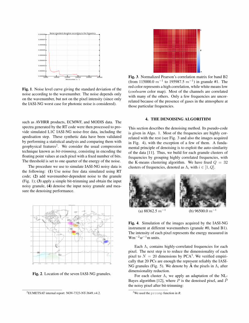
(a) 88362.5 m−1 (b) 96500.0 m−1

Fig. 4. Simulation of the images acquired by the IASI-NGinstrument at different wavenumbers (granule #0, band B1).The intensity of each pixel represents the energy measured inWm−2sr−1m units.

Each Λi contains highly-correlated frequencies for eachpixel. The next step is to reduce the dimensionality of eachpixel to N = 20 dimensions by PCA3. We verified empiri-cally that 20 PCs are enough the represent reliably the IASI-NG granules (Fig. 5). We denote by A the pixels in Λi afterdimensionality reduction.

For each cluster Λi we apply an adaptation of the NL-Bayes algorithm [12], where P is the denoised pixel, and Pthe noisy pixel after bit-trimming:

3We used the prcomp function in R.

0 10 20 30 40 50Index of sorted abs. eigenvalue

16

14

12

10

8

6

4

2

0lo

g o

f th

e norm

aliz

ed e

xpla

ined

var

iance

Explained variance

Fig. 5. Decay of the normalized explained variance accordingto the sorted eigenvalues, in log scale.

P = P + [CP −Cn]C−1

P

(P − P

). (1)

CP is the empirical covariance matrix of the most similarpixels in the cluster. We use the Pearson’s correlation coef-ficient as the similarity criterion4. The empirical covariancematrix Cn of the bit-trimmed noise after PCA transforma-tion is required too. It needs to be computed only for thewavenumbers in Λi. Sec. 4.1 gives the details on how tocompute Cn. For each cluster Λi, the NL-Bayes algorithm isapplied. Since each cluster contains only a part of the totalset of wavenumbers, each pixel is denoised partly at each it-eration. After all iterations, the pixel is completely denoised.Finally, the denoised pixels are unprojected (the data is ex-pressed in the same axes as before the PCA rotation) and thewhole denoised granule is obtained.

4.1. Calculation of Cn

In this section we explain how to calculate the empirical co-variance matrix of the noise Cn required in Eq. (1), underPCA axes rotation. Let us define N as an n × p matrix con-taining the noise. Each of the n rows corresponds to a par-ticular noisy pixel observation and each of the p columns toa variable (wavenumber) of the noisy pixel. The PCA re-quires that the data is centered. In practice, the barycen-ter of the set of noisy pixels is subtracted from each col-umn. In our case, since the noise has zero mean along anywavenumber, we can use directly N and compute its eigen-values and eigenvectors. We shall call W the p × p matrixwhich contains in its rows the normalized eigenvectors of N.Any wavenumber Fj with j ∈ [1, n] can be written in thePCA rotated axes as Fj = WNj . Thus, the entries of the co-variance matrix at [j1, j2] are cov (Fj1 ,Fj2) = E

(Fj1F

Tj2

)−

4It can be computed quickly with the corrcoef function in NumPy, forexample.

E (Fj1)E(FT

j2

)= E

(Fj1F

Tj2

)= E

(WFj1F

Tj2WT

)=

WE(Fj1F

Tj2

)WT .

We shall call D = E(Fj1F

Tj2

)=

{σ2j1

+ σ2Fj1

if j1 = j2

0 otherwise,and thus cov (Fj1 ,Fj2) = E

(WDWT

). The variance σ2

Fj1

is added because a bit-trimming compression is applied to thenoisy granule, which can be understood as adding a quantiza-tion noise. Let us define B (Fj) as the bit-trimming operatorapplied to the pixels in a given wavenumber Fj . Then,

σ2Fj

= var (|Fj − B (Fj) |) . (2)

Finally, the empirical covariance matrix of the noise in therotated PCA axes can be written as

Cn = WDWT . (3)

5. RESULTS

To measure the performance of our denoising method we de-fined the MSNR5 metric as:

MSNRj(T,G) = 10 log10

[median(Tj)

2

MSE(Tj ,Gj)

], (4)

where j is a given wavenumber, T the testing granule, G thereference noise-free granule, and MSE stands for the MeanSquared Error. Note that the formula (4) is the same as theusual PSNR for a wavenumber j, with the difference that weuse the median of the noisy granule instead of its maximumvalue. The reason is to avoid the effect of outlier values whichwould bias the measurement of performance.

Fig. 6 shows the MSNR plots of two granules6 and com-pares the MSNR of the noise (red), with our denoising method(green), and the results obtaining by simply performing PCAand keeping the N = 20 most significant PCs. As it can beobserved, since the signal is highly correlated (see Fig. 3),simply applying PCA and keeping the most significant PCsis an effective strategy. However, combining dimensionalityreduction with Bayesian denoising improves significantly theresult.

Table 1 shows the square root of the ratio between theMSEs of the noisy and denoised granules with respect to thenoise-free granule.

5Median Signal-to-Noise Ratio.6Similar results are obtained with the other granules.

0 2000 4000 6000 8000 10000 12000 14000 16000 18000Channel index

20

0

20

40

60

80M

SN

R (

dB)

MSNR with noiseFree

noisydenoised oursdenoised PCA

(a) Granule #2

0 2000 4000 6000 8000 10000 12000 14000 16000 18000Channel index

20

0

20

40

60

80

MSN

R (

dB)

MSNR with noiseFree

noisydenoised oursdenoised PCA

(b) Granule #5

Fig. 6. MSNR denoising performances of two of the sevengranules analyzed. The reference is the noise-free granulewithout bit-trimming. In red: the MSNR corresponding to thenoisy granule without bit-trimming. In green: the MSNR ofour denoising method, with bit-trimming. In blue: the de-noising result only applying PCA dimension reduction withN = 20 principal components, with bit-trimming. Since thecurves oscillate much, they have been filtered with a Gaussianof σ = 50 for visualization and comparison purposes.

6. CONCLUSIONS

We have presented a new method to denoise hyperspectral3D images. This method has been successfully applied tosimulated IASI-NG spectra. IASI and IASI-NG data havebeen used as example to demonstrate the denoising capabili-ties and to illustrate the difficulties. However, the method isgeneral enough to be applied to other types of HS images bychoosing the right parameters {Q,K,N} in Algo. 1. Themethod is unsupervised and uses several techniques to adaptto the data of each particular granule: first it creates clus-ters of frequencies to group data supposed to come from thesame physical origin, then it reduces the dimensionality of thedata by means of PCA based on the data of the granule, andfinally it uses another kind of clustering (in this case basedof inter-pixel correlation) to denoise the granule. The modelfor the data (in the form of the covariance matrix of similarpixels, CP ) is learned from the input granule itself instead

Granule #0 #1 #2 #3 #4 #5 #6√MSE(B(G),G)

MSE(G,G)3.53 4.73 4.25 4.79 4.23 3.49 4.85

Table 1. Denoising gain as the square root of the ratio be-tween the MSEs of the bit-trimmed noisy and denoised gran-ules with respect to the noise-free granule. Average: 4.27.

Algorithm 1 Denoise a IASI-NG hyperspectral image1: Denoising

Input G: acquired noisy granuleInput Q = 32: number of spectral clustersInput K = 400: number of similar pixelsInput N = 20: number of PCA PCs keptOutput G: denoised granule

2: G = zeros(G.shape) . Placeholder3: Split the spectrum into Q frequential clusters Λi, i ∈ [1, Q]4: for each cluster Λi, i ∈ [1, Q] do5: A = PCA(Λi, N) . Reduce dimensionality to N variables6: Compute the covariance matrix Cn of the noise . Eq. (3)7: for each noisy pixel P do8: For the K most correlated pixels compute: (i) their mean

P and (ii) their covariance matrix CP

9: Obtain the denoised pixel P using NL-Bayes . Eq. (1)10: A← P . Store denoised P11: end for12: G(Λi)← UNPROJECT(A) . Back to the original axes13: end for14: return G

of using a predefined model. The use of dimensionality re-duction has two main benefits: first, after projection on thePCA basis, the underlying signal and the noise are much sep-arated, which allows a better comparison of the pixels takinginto account the signal in the first N = 20 PCs and not thenoise. This can be understood as some kind of oracle tech-nique to find similar pixels, in analogy with explicitly oracularmethods like BM3D [13] . In our case, it is done implicitly.The second benefit is that the drastic dimensionality reduc-tion (from 16923 spectral channels to N = 20 PCs) speedsup significantly the computations.

The quantitative results show that the combination of thebi-clustering, dimensionality reduction, and Bayesian denois-ing implies a gain in several dBs with respect to simply keep-ing the most significant PCA PCs. The reduction of the noisein a factor of 4 shown in Table 1 means that the surface of thecaptor could be reduced in a factor 16 while keeping the sameperformance. As future work, we aim to obtain denoising re-sults for existing real IASI satellite images and use differentmetrics to evaluate the denoising performance, as for examplethe inter-channel correlation and the off-diagonal coefficientsof the noise covariance matrix before and after denoising.

7. REFERENCES

[1] C. Crevoisier, C. Clerbaux, V. Guidard, T. Phulpin,R. Armante, B. Barret, Camy-Peyret C., J. P.Chaboureau, P. F. Coheur, L. Crepeau, et al., “To-wards IASI-new generation (IASI-NG): impact of im-proved spectral resolution and radiometric noise on theretrieval of thermodynamic, chemistry and climate vari-ables,” Atmospheric Measurement Techniques, vol. 7,no. 12, pp. 4367–4385, 2014.

[2] Cyril Crevoisier, Cathy Clerbaux, Vincent Guidard, EricPequignot, and Frederick Pasternak, “IASI-NG: unconcentre d’innovations technologiques pour l’etude del’atmosphere terrestre,” La Meteorologie, , no. 86, pp.3–5, 2014.

[3] F. Bernard, B. Calvel, F. Pasternak, R. Davancens,C. Buil, E. Baldit, C. Luitot, and A. Penquer, “Overviewof IASIw-NG the new generation of infrared atmo-spheric sounder,” in International Conference on SpaceOptics, 2014, vol. 7, p. 10.

[4] Bormin Huang, Hung-Lung A Huang, Alok Ahuja, Tim-othy J. Schmit, and Roger W. Heymann, “Lossless datacompression for infrared hyperspectral sounders: an up-date,” in Optical Science and Technology, the SPIE 49thAnnual Meeting. International Society for Optics andPhotonics, 2004, pp. 109–119.

[5] Guangyi Chen and Shen-En Qian, “Denoising of hy-perspectral imagery using principal component analysisand wavelet shrinkage,” Geoscience and Remote Sens-ing, IEEE Transactions on, vol. 49, no. 3, pp. 973–980,2011.

[6] Behnood Rasti, Johannes R Sveinsson, Magnus O Ul-farsson, and Jon Atli Benediktsson, “Hyperspectral im-age denoising using 3d wavelets,” in Geoscience andRemote Sensing Symposium (IGARSS), 2012 IEEE In-ternational. IEEE, 2012, pp. 1349–1352.

[7] P. Antonelli, H. E. Revercomb, L. A. Sromovsky, W. L.Smith, R. O. Knuteson, D. C. Tobin, R. K. Garcia, H. B.Howell, H. L. Huang, and F. A. Best, “A principal com-ponent noise filter for high spectral resolution infraredmeasurements,” Journal of Geophysical Research: At-mospheres, vol. 109, no. D23, 2004.

[8] A. D. Collard, A. P. McNally, F. I. Hilton, S. B. Healy,and N. C. Atkinson, “The use of principal componentanalysis for the assimilation of high-resolution infraredsounder observations for numerical weather prediction,”Quarterly Journal of the Royal Meteorological Society,vol. 136, no. 653, pp. 2038–2050, 2010.

[9] Jean-Michel Gaucel, Carole Thiebaut, Romain Hugues,and Roberto Camarero, “On-board compression of hy-perspectral satellite data using band-reordering,” inSPIE Optical Engineering+ Applications. InternationalSociety for Optics and Photonics, 2011, pp. 81570W–81570W.

[10] Giuseppe Grieco, Carmine Serio, and Guido Masiello,“σ-IASI-β: a hyperfast radiative transfer code to re-trieve surface and atmospheric geophysical parameters,”EARSeL eProceedings, vol. 12, no. 2, pp. 149, 2013.

[11] M. Lebrun, M. Colom, A. Buades, and J. M. Morel, “Se-crets of image denoising cuisine,” Acta Numerica, vol.21, no. 1, pp. 475–576, 2012.

[12] Marc Lebrun, Antoni Buades, and Jean-Michel Morel,“A nonlocal Bayesian image denoising algorithm,”SIAM Journal on Imaging Sciences, vol. 6, no. 3, pp.1665–1688, 2013.

[13] Kostadin Dabov, Alessandro Foi, Vladimir Katkovnik,and Karen Egiazarian, “Image denoising by sparse 3-dtransform-domain collaborative filtering,” Image Pro-cessing, IEEE Transactions on, vol. 16, no. 8, pp. 2080–2095, 2007.

Acknowledgement: Centre National d’Etudes Spatiales (CNES,R&T action), EUMETSAT, European Research Council (AdvancedGrant Twelve Labours), Office of Naval Research (Grant N00014-97-1-0839), Direction Generale de l’Armement (DGA).